oscillations and warming trend in global temperature time seriesabhishek/geo-project.pdf ·...
TRANSCRIPT
Oscillations and Warming Trend inGlobal Temperature time series
-Abhishek Bhattacharya
1
Introduction
• The goal of this project is to distinguish
a warming trend and periodic oscillations
from natural variability in global surface air
temperatures.
• First I use a Singular Value decompo-
sition (SVD) analysis of the three dimen-
sional temperature data over different sta-
tions all over the world and over differ-
ent months. That gives the leading spa-
tial patterns explaining most of the vari-
ation. Since those patterns concentrate
mostly over the North Atlantic region, I
focus on the analysis of that region. I use
the leading patterns to reconstruct the an-
nual average temperature over the North
Atlantic.
2
• Then I use Singular Spectrum Analysis
(SSA) to analyze the time series of an-
nual average surface air temperatures over
North Atlantic for the past 136 years, al-
lowing a secular warming trend and a small
number of oscillatory modes to be sepa-
rated from the noise. There is a rising
trend since 1910. The oscillations exhibit
periods of around 5 or 6 years.
3
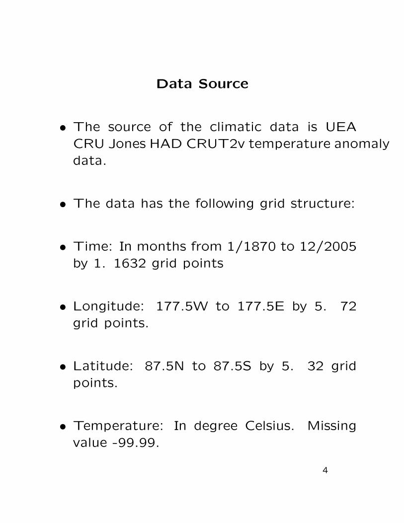
Data Source
• The source of the climatic data is UEA
CRU Jones HAD CRUT2v temperature anomaly
data.
• The data has the following grid structure:
• Time: In months from 1/1870 to 12/2005
by 1. 1632 grid points
• Longitude: 177.5W to 177.5E by 5. 72
grid points.
• Latitude: 87.5N to 87.5S by 5. 32 grid
points.
• Temperature: In degree Celsius. Missing
value -99.99.
4
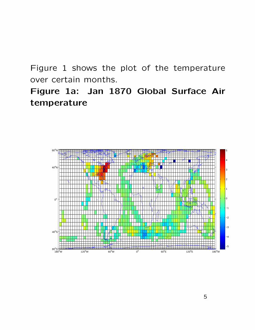
Figure 1 shows the plot of the temperature
over certain months.
Figure 1a: Jan 1870 Global Surface Air
temperature
180oW 120oW 60oW 0o 60oE 120oE 180oW 80oS
40oS
0o
40oN
80oN
−5
−4
−3
−2
−1
0
1
2
3
4
5
5
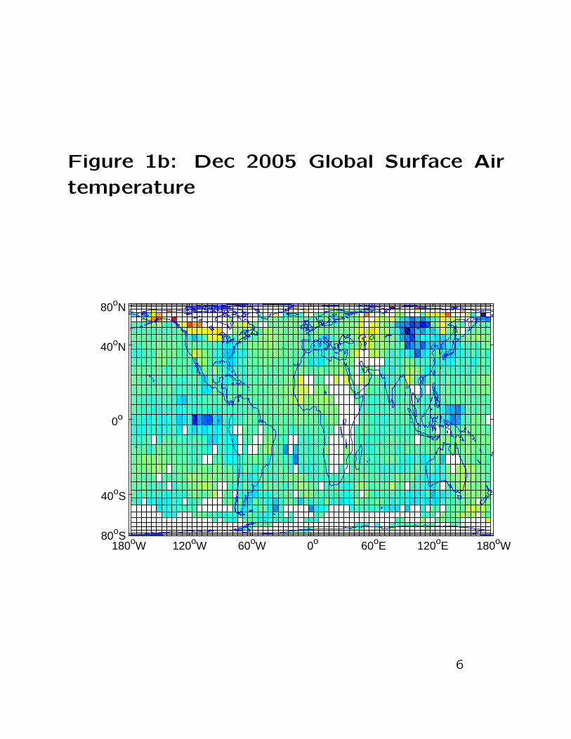
Figure 1b: Dec 2005 Global Surface Air
temperature
180oW 120oW 60oW 0o 60oE 120oE 180oW 80oS
40oS
0o
40oN
80oN
6
Empirical Orthogonal Function (EOF)
decomposition Analysis
• Prior to the analysis, I weight the data ap-
propriately to take into account the distor-
tion in high latitudes in a Mercator projec-
tion. I apply weights to the grid points, the
weight being proportional to the cosine of
the latitude.
• Then I compute the spatial covariance ma-
trix. To have significant number of obser-
vations, I use the last 100 years: 01/1906
to 12/2005 in my covariance calculation.
Also I use only those grid points which have
at least 50 years of data. That would en-
sure that the pairs have at least 5 years of
overlap.
7
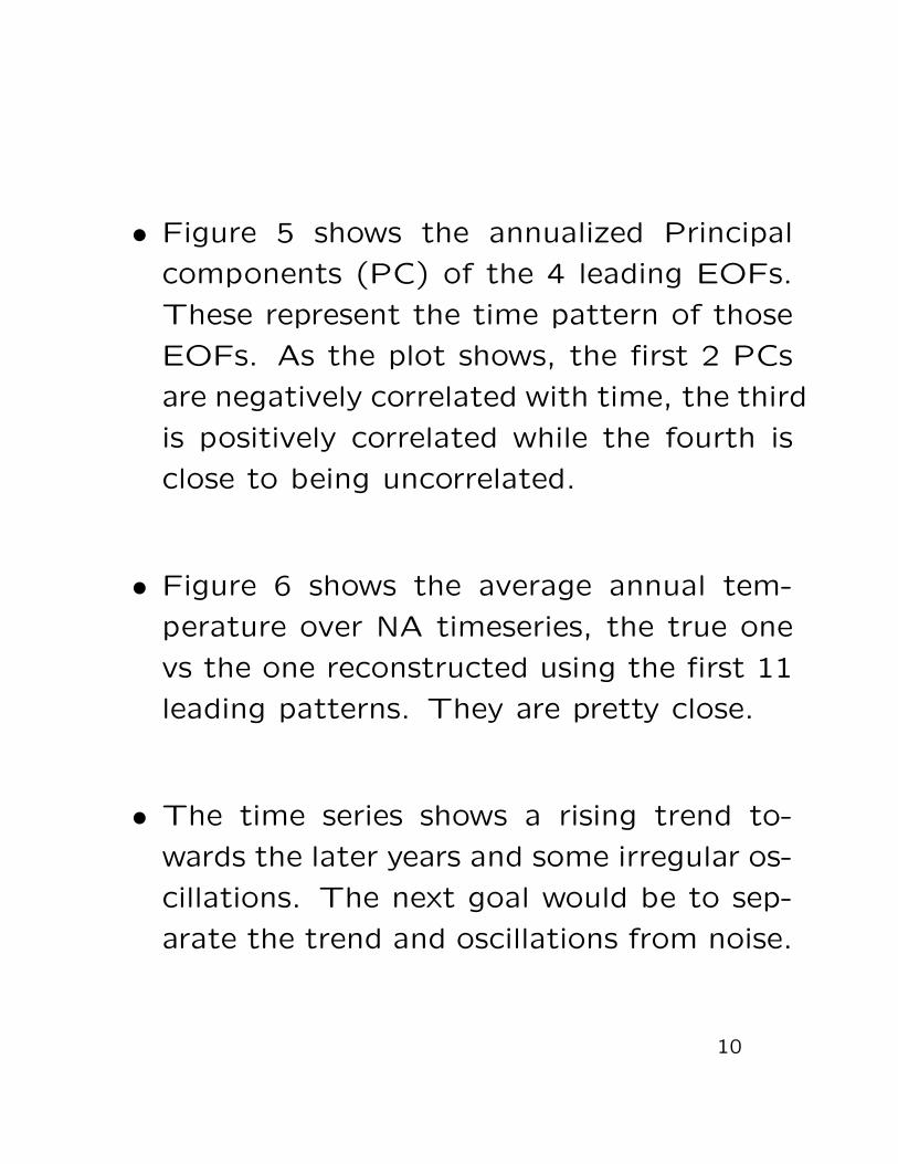
• Figure 2 shows the grid points used in my
analysis. Most of them concentrate around
Northern Atlantic (NA).
• Then I compute the eigen vectors and eigen
values of the covariance matrix.
• Figure 3 shows the spatial pattern of the
first four EOFs. All of them concentrate
on NA and have a single pole in that re-
gion. EOFs 1 and 2 are positive correlated
with space while EOFs 3 and 4 are close
to negative. They explain 22, 13, 9 and 7
percent of the variation in the data respec-
tively. Together they explain about 51% of
the variance.
• Since the EOF plots are very localized,
they explain the spatial directions well.
8
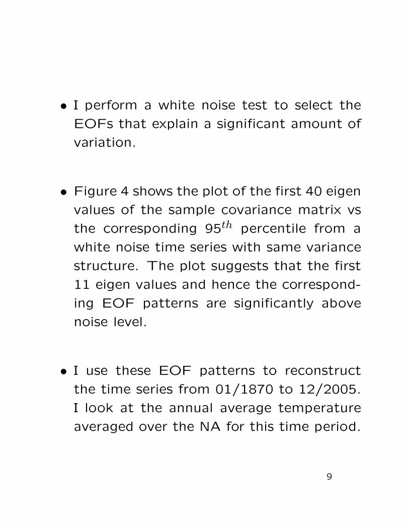
• I perform a white noise test to select the
EOFs that explain a significant amount of
variation.
• Figure 4 shows the plot of the first 40 eigen
values of the sample covariance matrix vs
the corresponding 95th percentile from a
white noise time series with same variance
structure. The plot suggests that the first
11 eigen values and hence the correspond-
ing EOF patterns are significantly above
noise level.
• I use these EOF patterns to reconstruct
the time series from 01/1870 to 12/2005.
I look at the annual average temperature
averaged over the NA for this time period.
9
• Figure 5 shows the annualized Principal
components (PC) of the 4 leading EOFs.
These represent the time pattern of those
EOFs. As the plot shows, the first 2 PCs
are negatively correlated with time, the third
is positively correlated while the fourth is
close to being uncorrelated.
• Figure 6 shows the average annual tem-
perature over NA timeseries, the true one
vs the one reconstructed using the first 11
leading patterns. They are pretty close.
• The time series shows a rising trend to-
wards the later years and some irregular os-
cillations. The next goal would be to sep-
arate the trend and oscillations from noise.
10
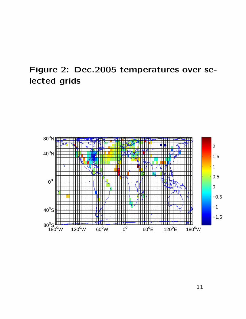
Figure 2: Dec.2005 temperatures over se-
lected grids
180oW 120oW 60oW 0o 60oE 120oE 180oW 80oS
40oS
0o
40oN
80oN
−1.5
−1
−0.5
0
0.5
1
1.5
2
11
Figure 3: The first 4 EOF patterns
3a. EOF−1 Pattern
180oW 120oW 60oW 0o 60oE 120oE 180oW 80oS
40oS
0o
40oN
80oN 3b. EOF−2 Pattern
180oW 120oW 60oW 0o 60oE 120oE 180oW 80oS
40oS
0o
40oN
80oN
3c. EOF−3 Pattern
180oW 120oW 60oW 0o 60oE 120oE 180oW 80oS
40oS
0o
40oN
80oN 3d. EOF−4 Pattern
180oW 120oW 60oW 0o 60oE 120oE 180oW 80oS
40oS
0o
40oN
80oN
−0.2
−0.1
0
0.1
0.2
0.3
12
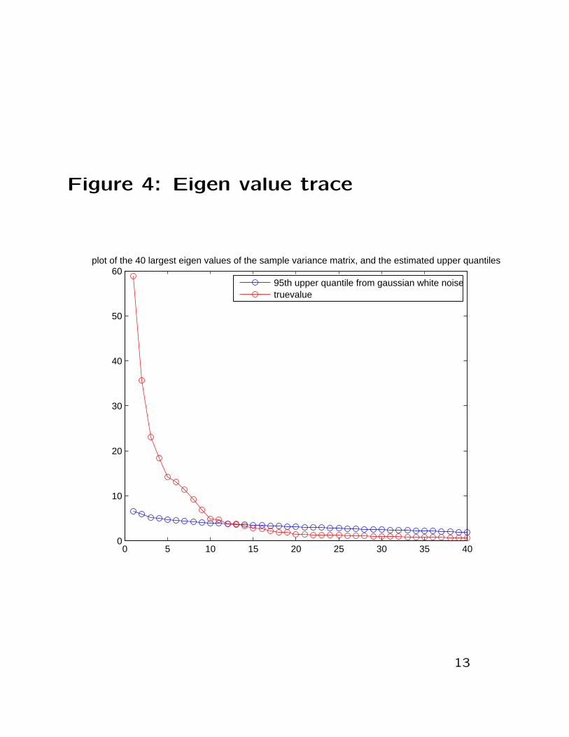
Figure 4: Eigen value trace
0 5 10 15 20 25 30 35 400
10
20
30
40
50
60plot of the 40 largest eigen values of the sample variance matrix, and the estimated upper quantiles
95th upper quantile from gaussian white noisetruevalue
13
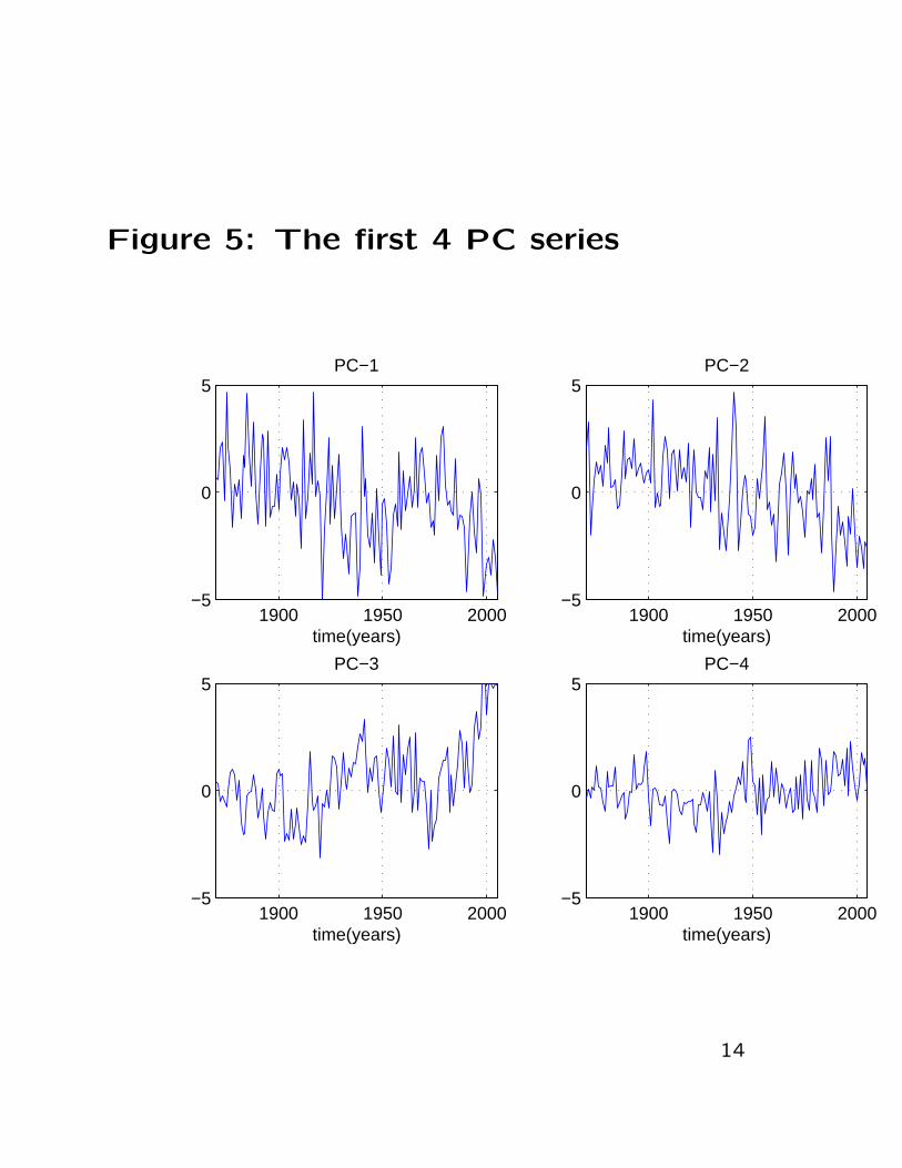
Figure 5: The first 4 PC series
1900 1950 2000−5
0
5
time(years)
PC−1
1900 1950 2000−5
0
5
time(years)
PC−2
1900 1950 2000−5
0
5
time(years)
PC−3
1900 1950 2000−5
0
5
time(years)
PC−4
14
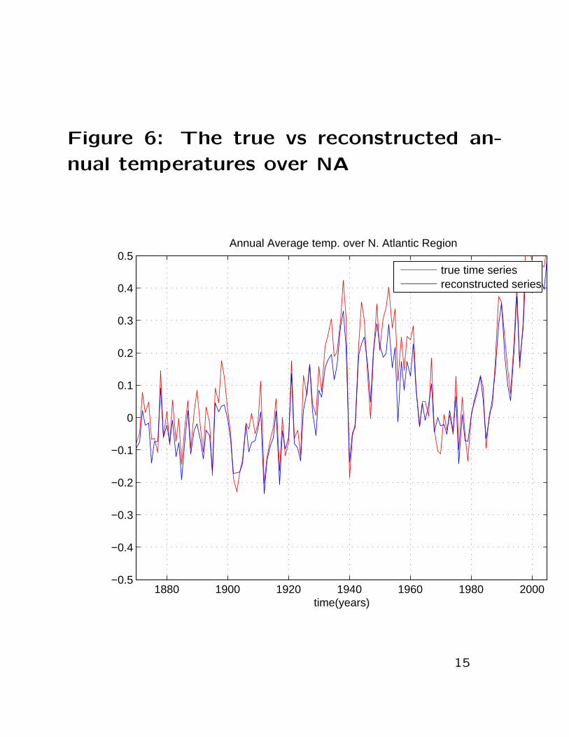
Figure 6: The true vs reconstructed an-
nual temperatures over NA
1880 1900 1920 1940 1960 1980 2000−0.5
−0.4
−0.3
−0.2
−0.1
0
0.1
0.2
0.3
0.4
0.5Annual Average temp. over N. Atlantic Region
time(years)
true time seriesreconstructed series
15
Singular Spectrum Analysis (SSA) of
annual temperatures over NA
• Now I develop a SSA of the reconstructed
time series of annual temperature data over
NA from 01/1870 to 12/2005.
• I choose an embedding dimension, m, com-
pute the covariance matrix of the embed-
ded data set, calculate its eigen values,
eigen vactors and reconstructed components
for the time series.
• I compare the eigen values with those from
a white noise process to check their signif-
icance at level 95%.
16
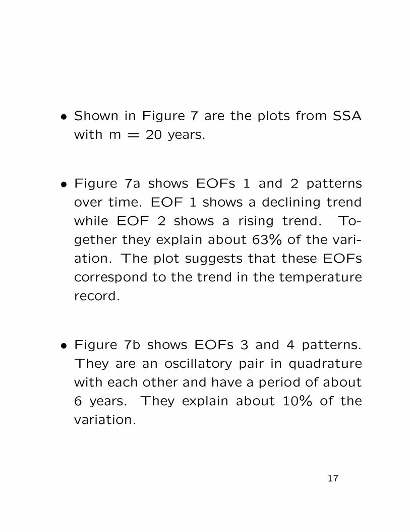
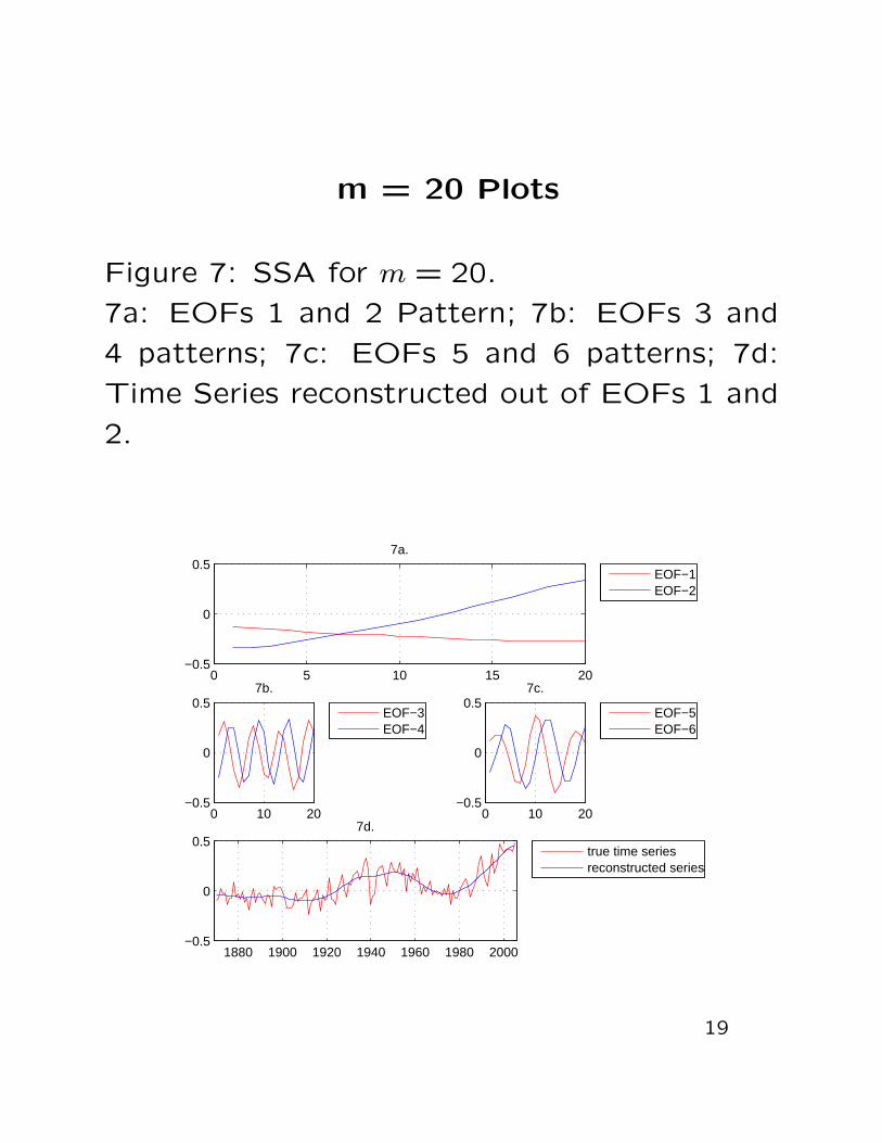
• Shown in Figure 7 are the plots from SSA
with m = 20 years.
• Figure 7a shows EOFs 1 and 2 patterns
over time. EOF 1 shows a declining trend
while EOF 2 shows a rising trend. To-
gether they explain about 63% of the vari-
ation. The plot suggests that these EOFs
correspond to the trend in the temperature
record.
• Figure 7b shows EOFs 3 and 4 patterns.
They are an oscillatory pair in quadrature
with each other and have a period of about
6 years. They explain about 10% of the
variation.
17
• Figure 7c shows the EOFs 5 and 6. They
also form oscillatory pairs in quadrature with
each other and have a period of about 10
years. They explain about 8% of the vari-
ation.
• In Figure 7d is shown the time series recon-
structed out of the first two EOFs. The
trend is flat until 1910 and then a rise after
that.
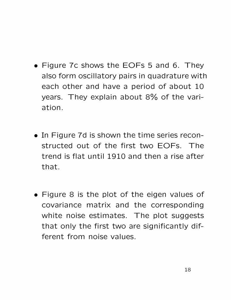
• Figure 8 is the plot of the eigen values of
covariance matrix and the corresponding
white noise estimates. The plot suggests
that only the first two are significantly dif-
ferent from noise values.
18
m = 20 Plots
Figure 7: SSA for m = 20.
7a: EOFs 1 and 2 Pattern; 7b: EOFs 3 and
4 patterns; 7c: EOFs 5 and 6 patterns; 7d:
Time Series reconstructed out of EOFs 1 and
2.
0 5 10 15 20−0.5
0
0.57a.
EOF−1EOF−2
0 10 20−0.5
0
0.57b.
EOF−3EOF−4
0 10 20−0.5
0
0.57c.
EOF−5EOF−6
1880 1900 1920 1940 1960 1980 2000−0.5
0
0.57d.
true time seriesreconstructed series
19
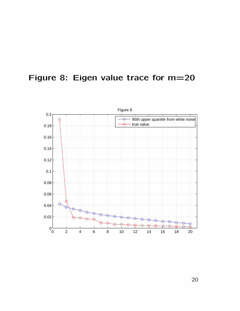
Figure 8: Eigen value trace for m=20
0 2 4 6 8 10 12 14 16 18 200
0.02
0.04
0.06
0.08
0.1
0.12
0.14
0.16
0.18
0.2Figure 8
95th upper quantile from white noisetrue value
20
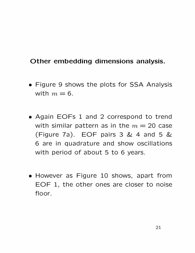
Other embedding dimensions analysis.
• Figure 9 shows the plots for SSA Analysis
with m = 6.
• Again EOFs 1 and 2 correspond to trend
with similar pattern as in the m = 20 case
(Figure 7a). EOF pairs 3 & 4 and 5 &
6 are in quadrature and show oscillations
with period of about 5 to 6 years.
• However as Figure 10 shows, apart from
EOF 1, the other ones are closer to noise
floor.
21
• When m = 10 (Figure 11), EOFs 1 and
2 correspond to trend; EOFs 3 & 4 are
in quadrature with period around 6 years;
EOF 5 has period of 10 years while EOF
6 shows a noisy pattern.
• In Figure 12, again only EOF 1 is signifi-
cantly above noise floor.
• When m = 30 (Figure 13), EOFs 1 and
2 correspond to trend; EOFs 3 & 4 are
in quadrature with period around 6 years;
EOFs 5 & 6 are in quadrature with period
around 6 years. In Figure 14, EOFs 1 & 2
are significantly above noise level.
22
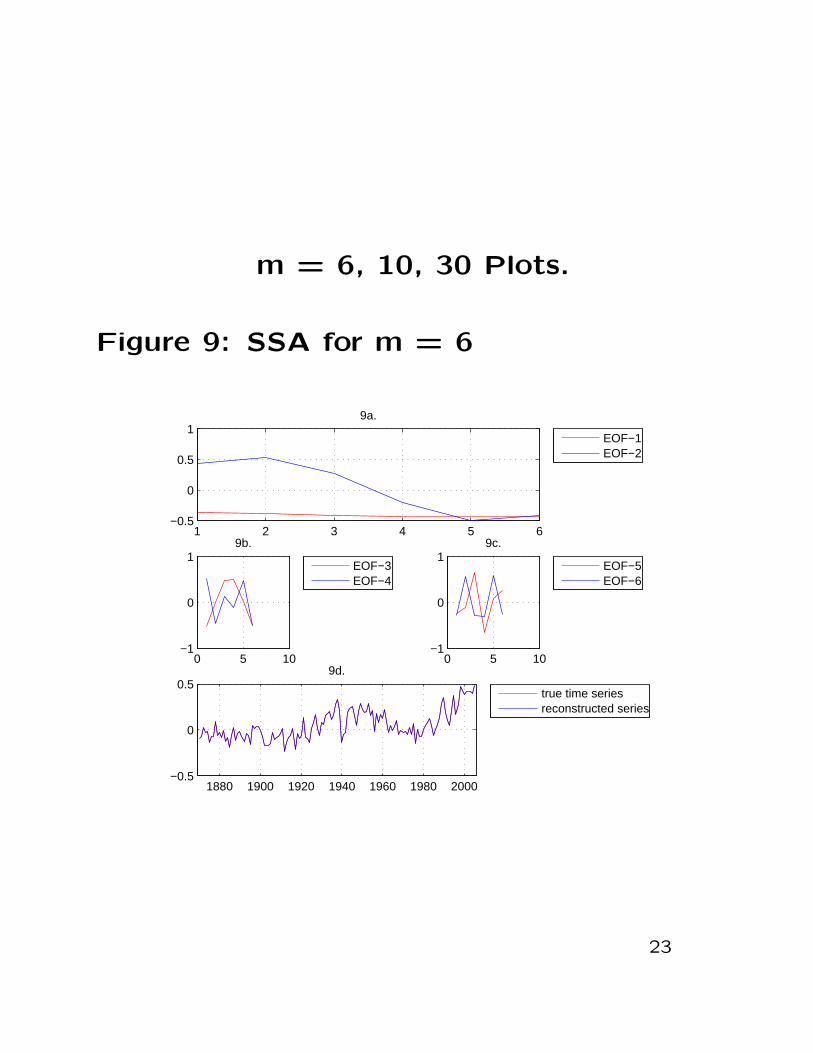
m = 6, 10, 30 Plots.
Figure 9: SSA for m = 6
1 2 3 4 5 6−0.5
0
0.5
19a.
EOF−1EOF−2
0 5 10−1
0
19b.
EOF−3EOF−4
0 5 10−1
0
19c.
EOF−5EOF−6
1880 1900 1920 1940 1960 1980 2000−0.5
0
0.59d.
true time seriesreconstructed series
23
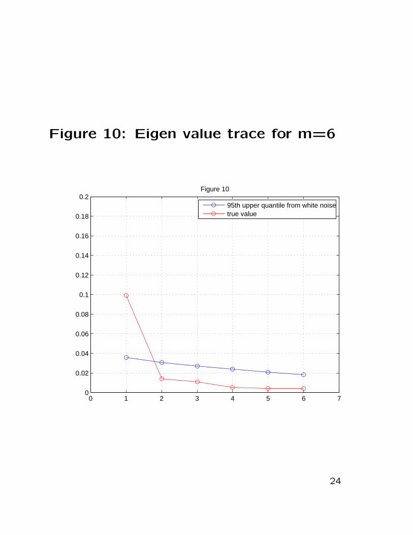
Figure 10: Eigen value trace for m=6
0 1 2 3 4 5 6 70
0.02
0.04
0.06
0.08
0.1
0.12
0.14
0.16
0.18
0.2Figure 10
95th upper quantile from white noisetrue value
24
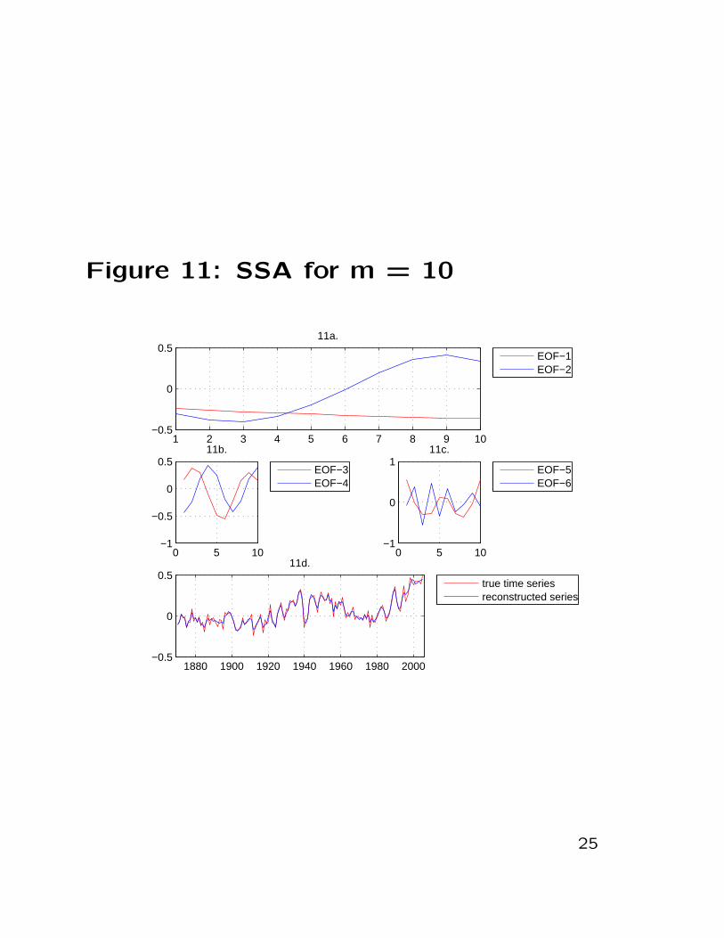
Figure 11: SSA for m = 10
1 2 3 4 5 6 7 8 9 10−0.5
0
0.511a.
EOF−1EOF−2
0 5 10−1
−0.5
0
0.511b.
EOF−3EOF−4
0 5 10−1
0
111c.
EOF−5EOF−6
1880 1900 1920 1940 1960 1980 2000−0.5
0
0.511d.
true time seriesreconstructed series
25
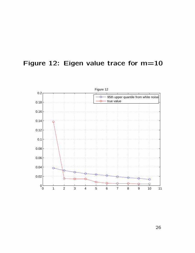
Figure 12: Eigen value trace for m=10
0 1 2 3 4 5 6 7 8 9 10 110
0.02
0.04
0.06
0.08
0.1
0.12
0.14
0.16
0.18
0.2Figure 12
95th upper quantile from white noisetrue value
26
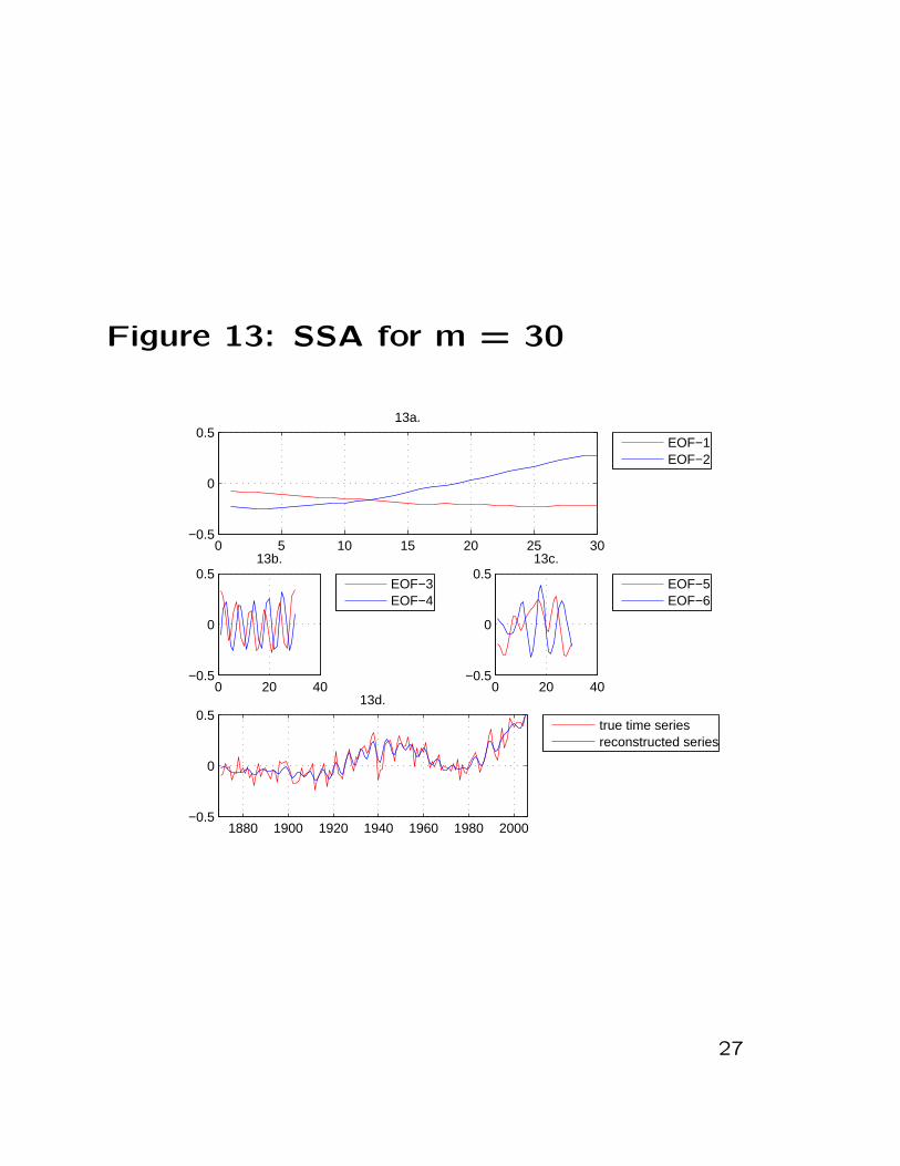
Figure 13: SSA for m = 30
0 5 10 15 20 25 30−0.5
0
0.513a.
EOF−1EOF−2
0 20 40−0.5
0
0.513b.
EOF−3EOF−4
0 20 40−0.5
0
0.513c.
EOF−5EOF−6
1880 1900 1920 1940 1960 1980 2000−0.5
0
0.513d.
true time seriesreconstructed series
27
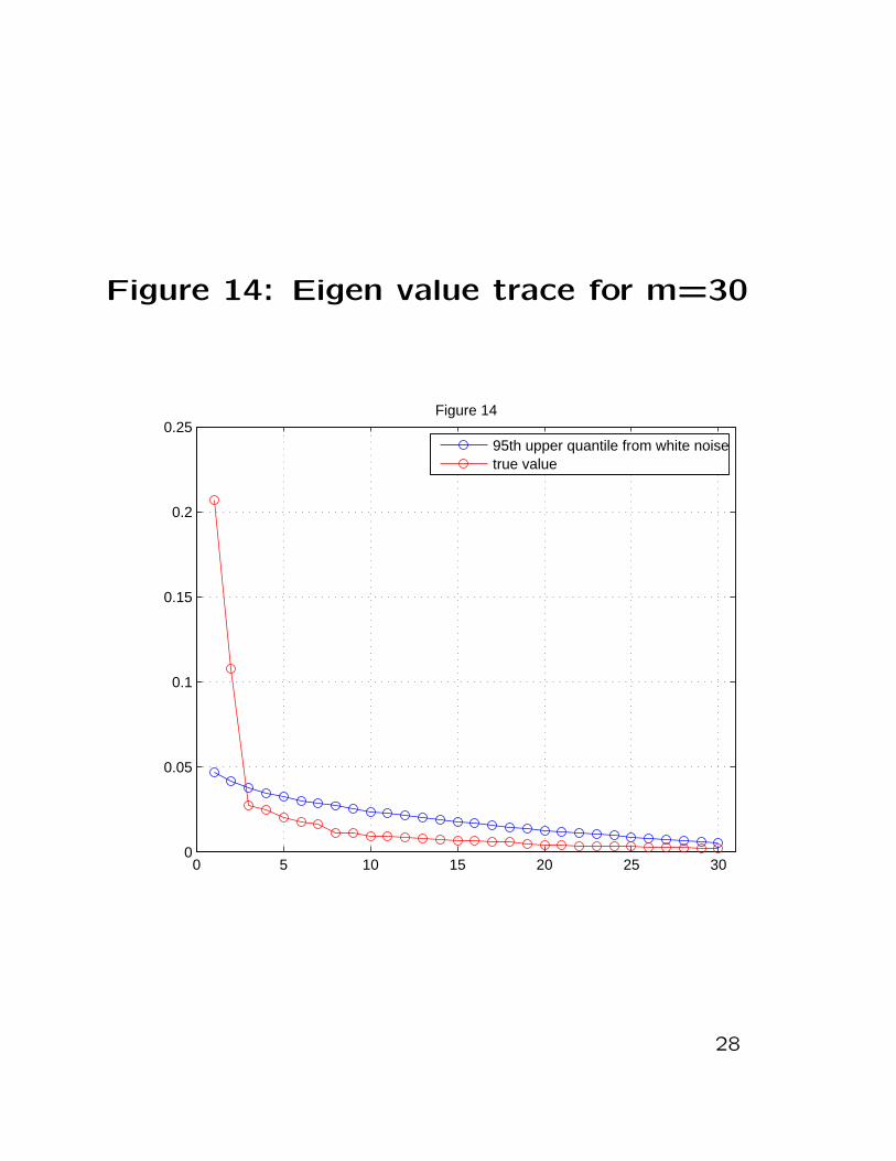
Figure 14: Eigen value trace for m=30
0 5 10 15 20 25 300
0.05
0.1
0.15
0.2
0.25Figure 14
95th upper quantile from white noisetrue value
28
Sensitivity of SSA to choice of
embedding dimension, m
• Now I check how robust is the SSA analy-
sis.
• As all eigen value trace plots in Figures 10
(m = 6), 12 (m = 10), 8 (m = 20) and 14
(m = 30) show, there is a sharp fall from
eigen value 1 to 2, another less sharper fall
from eigen values 2 to 3 after which the
trace gets flat.
29
• Also we see that as m increases, the trace
gets steeper. This suggests stationarity in
the data. If the series were truly station-
ary, the covariance matrix for a smaller m
can be ”roughly” embedded into that for
a larger m. Then the latter will have its
largest eigen values bigger, while the least
eigen values smaller, leading to a steeper
eigen value trace.
• Since the first two EOFs represent trend
and the next two periodicity for all dimen-
sions, I reconstruct the time series using
these EOFs for m = 5,6,10,12,20,30,50
and 100 years. In each case I compute
the correlation of the summed components
with that for m = 20.
30
• Figure 15a shows the plot of the correla-
tions. The plot shows that the correlation
is over 0.8 for m < 80. This suggests that
the different values of m less than 80 do
not substatantially alter the SSA analysis
results.
• In Figure 15b is plotted the variance ex-
plained by the first four EOFs for the above
values of m. The plot is rising which sup-
ports my earlier claim about stationarity,
and the rise is fairly smooth till m = 60
suggesting robustness of the analysis for
m < 60.
• Figure 15c shows the plot of the fractional
variance explained by the first 4 EOFs vs
the embedding dimension, m. This plot is
declining. The values are over 50% in all
case, and over 60% for m < 60.
31
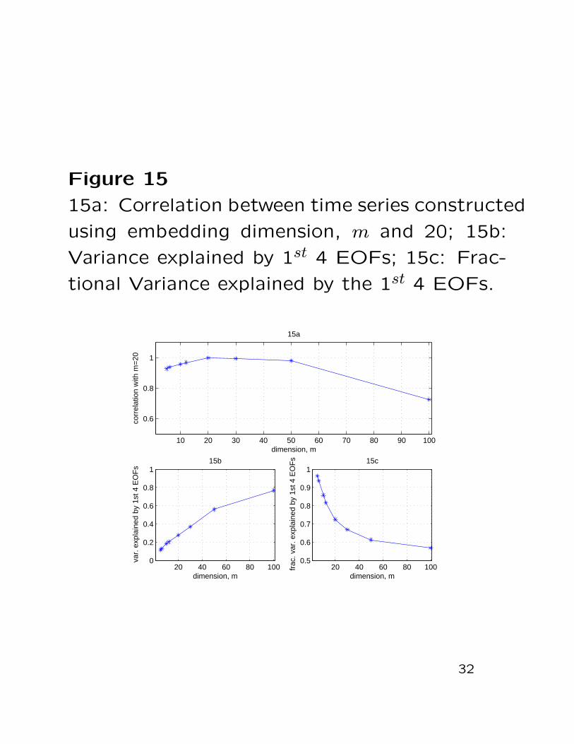
Figure 15
15a: Correlation between time series constructed
using embedding dimension, m and 20; 15b:
Variance explained by 1st 4 EOFs; 15c: Frac-
tional Variance explained by the 1st 4 EOFs.
10 20 30 40 50 60 70 80 90 100
0.6
0.8
1
15a
dimension, m
corr
elat
ion
with
m=
20
20 40 60 80 1000
0.2
0.4
0.6
0.8
115b
dimension, m
var.
exp
lain
ed b
y 1s
t 4 E
OF
s
20 40 60 80 1000.5
0.6
0.7
0.8
0.9
115c
dimension, m
frac
. var
. exp
lain
ed b
y 1s
t 4 E
OF
s
32
Conclusions
• From different dimensional SSA analysis,
we observe that the EOFs 1 and 2 repre-
sent the trend in the data. As the true
and reconstructed timeseries show (Figure
7a), there has been a rise in surface air
temperatures since 1910. The estimation
of EOFs 1 and 2 is robust, in the sense
that their trend changes little with varying
dimension, m.
• EOFs 3 and 4 explain the major periodic-
ity in the data. They have a period be-
tween 5 and 6 years. However their esti-
mation is not so robust. Their trace pat-
tern varies with m. This is justified by the
fact that the corresponding eigen values
are very near to the noise floor for all m.
33
• The analysis shows no sign of bidecadal
oscillations as reported by Ghil and Vautard
[2].
• This raises the question whether a mini-
mum sample size is required to detect them.
However a sample size of 136 years seems
fairly large.
• Another reason could be, as Elsner and
Tsonis [1] point out, the years before 1881
made the difference. I get the leading pat-
terns from the EOF analysis of the covari-
ance matrix constructed using the past 100
years: 1906 to 2005 and use those to re-
construct the annual average temperature
over NA time series for the span of past
136 years (1870-2005). Perhaps including
the earliest years in calculating the EOFs
would make a difference.
34
• However that would mean that the data is
non stationary while SSA is designed mainly
for stationary data.
• This makes one doubt the existence of bidecadal
oscillations in the temperature records, and
the tools used to detect them.
35
References
[1] ELSNER, J.B. and TSONIS, A.A.(1991)
Do bidecadal oscillations exist in the global
temperature record? Nature353 551-553
[2] VAUTARD, R. and GHIL, M.(1991) Inter-
decadal oscillations and the warming trend
in global temperature time series. Nature350
324-327
[3] JONES, P.D. and MOBERG, A.(2003) Hemi-
spheric and large-scale surface air temper-
ature variations: an extensive revision and
an update to 2001. J.Climate16 206-223
36