PNNL-18945 Prepared for the U.S. Department of Energy under Contract DE-AC05-76RL01830

N Zhou F Tuffner Z Huang S Jin October 2009

Oscillation Detection Algorithm Development Summary Report and Test Plan

PNNL-18945

Oscillation Detection Algorithm Development Summary Report and Test Plan N Zhou F Tuffner Z Huang S Jin October 2009 Prepared for the U.S. Department of Energy under Contract DE-AC05-76RL01830 Pacific Northwest National Laboratory Richland, Washington 99352

iii

Preface

The California Energy Commission’s Public Interest Energy Research (PIER) Program supports public interest energy research and development that will help improve the quality of life in California by bringing environmentally safe, affordable, and relia-ble energy services and products to the marketplace.

The PIER Program conducts public interest research, development, and demonstration (RD&D) projects to benefit California.

The PIER Program strives to conduct the most promising public interest energy research by partnering with RD&D entities, including individuals, businesses, utilities, and public or private research institutions.

• PIER funding efforts are focused on the following RD&D program areas:

• Buildings End‐Use Energy Efficiency

• Energy Innovations Small Grants

• Energy‐Related Environmental Research

• Energy Systems Integration

• Environmentally Preferred Advanced Generation

• Industrial/Agricultural/Water End‐Use Energy Efficiency

• Renewable Energy Technologies

• Transportation

Oscillation Detection Algorithm Development Summary Report & Test Plan is the interim report for the Oscillation Detection and Analysis (contract number: 500-07-037, work authorization number: TRP-08-07) conducted by Pacific Northwest National Laboratory. The information from this project contributes to PIER’s Energy Systems Integration Program.

For more information about the PIER Program, please visit the Energy Commission’s website at www.energy.ca.gov/research/ or contact the Energy Commission at 916‐654‐4878.

iv

EXECUTIVE SUMMARY Small signal stability problems are one of the major threats to grid stability and reliability in California and the western U.S. power grid. An unstable oscillatory mode can cause large-amplitude oscillations and may result in system breakup and large-scale blackouts. There have been several incidents of system-wide oscillations. Of them, the most notable is the August 10, 1996 western system breakup produced as a result of undamped system-wide oscillations. There is a great need for real-time monitor-ing of small-signal oscillations in the system. In power systems, a small-signal oscillation is the result of poor electromechanical damping. Considerable understanding and literature have been developed on the small-signal stability problem over the past 50+ years. These studies have been mainly based on a linearized system model and eigenvalue analysis of its characteristic matrix. However, its practical feasibility is greatly limited because power system models have been found inadequate in describing real-time operating conditions. Significant efforts have been devoted to monitoring system oscillatory behaviors from real-time measurements in the past 20 years. The deployment of phasor measurement units (PMU) provides high-precision time-synchronized data needed for estimat-ing oscillation modes. Measurement-based modal analysis, also known as ModeMeter, uses real-time phasor measurements to estimate system oscillation modes and their damping. Low damping indicates potential system stability issues. Oscillation alarms can be issued when the power system is lightly damped. A good oscillation alarm tool can provide time for operators to take remedial reaction and reduce the probability of a system breakup as a result of a light damping condition. To facilitate ModeMeter development and evaluation, the Western Electricity Coordinating Council (WECC) has conducted a number of system tests in the past decade. The tests include large signal tests through insertion of the 1,400 MW Chief Joseph brake resis-tance, mid-level signal tests through ±125 MW modulation of Pacific DC Intertie (PDCI) real power set values, and noise prob-ing tests through ±10-20 MW modulation of the PDCI power. Recently, the system tests have advanced to a weekly basis, to-wards future continuous tests and real-time oscillation monitoring. Real-time oscillation monitoring requires ModeMeter algo-rithms to have the capability to work with various kinds of measurements: disturbance data (ringdown signals), noise probing data, and ambient data. Several measurement-based modal analysis algorithms have been developed. They include Prony analysis, Regularized Robust Recursive Least Square (R3LS) algorithm, Yule-Walker algorithm, Yule-Walker Spectrum algorithm, and the N4SID algorithm. Each has been shown to be effective for certain situations, but not as effective for some other situations. For example, the tradi-tional Prony analysis works well for disturbance data but not for ambient data, while Yule-Walker is designed for ambient data only. Even in an algorithm that works for both disturbance data and ambient data, such as R3LS, latency results from the time window used in the algorithm is an issue in timely estimation of oscillation modes. For ambient data, the time window needs to be longer to accumulate information for a reasonably accurate estimation; while for disturbance data, the time window can be significantly shorter so the latency in estimation can be much less. In addition, adding a known input signal such as noise prob-ing signals can increase the knowledge of system oscillatory properties and thus improve the quality of mode estimation. System situations change over time. Disturbances can occur at any time, and probing signals can be added for a certain time period and then removed. All these observations point to the need to add intelligence to ModeMeter applications. That is, a ModeMeter needs to adaptively select different algorithms and adjust parameters for various situations. This project aims to develop systematic approaches for algorithm selection and parameter adjustment. The very first step is to detect occurrence of oscillations so the algorithm and parameters can be changed accordingly. The proposed oscillation detec-tion approach is based on the signal-noise ratio of measurements. Intuitively, ambient data would have a low signal-noise ratio, while disturbance data would have a high signal-noise ratio. When the signal-noise ratio changes from a low value to a high value, the ModeMeter algorithm can be changed to use Prony analysis, or the time window of an algorithm can be greatly short-ened, so the latency is significantly reduced, and the responsiveness of mode estimation is improved. This report presents the oscillation detection approach and the plan for evaluating the approach as the next step of the project. The algorithm is based on signal-to-noise ratio (SNR) to detect ringdown oscillations. At this time, the algorithm has been im-plemented using MATLAB. Initial evaluation has been performed with simulation data from a 17-machine model and shows promising results similar to those shown in Figure 0-1. The plan is to perform further testing using field measurement data from WECC wide area measurement system (WAMS) to evaluate and improve the performance of the proposed algorithm. In addi-tion, a C++ based graphical user interface (GUI) is being developed for the algorithm.

v

Figure 0-1 Mean detection point and standard deviations of detection for 400 Monte-Carlo trials of 17th order/length and 20

dB event SNR

vi

ACKNOWLEDGEMENT

The preparation of this report was conducted with support from the California Energy Commission’s Public Interest Energy Re-search Program through the California Institute of Energy and Environment, and support from the Transmission Reliability Pro-gram of the Department of Energy’s Office of Electricity Delivery and Energy Reliability. Project support provided by Sue Arey and Kim Chamberlin, both with Pacific Northwest National Laboratory, is gratefully ac-knowledged. The Technical Advisory Committee for the project entitled “Oscillation Detection and Analysis”, funded by the California Energy Commission’s Public Interest Energy Research Program through the California Institute of Energy and Environment, consists of the following academic and industry experts:

• Jeff Dagle, Pacific Northwest National Laboratory • Soumen Ghosh, California Independent System Operator • Dmitry Kosterev, Bonneville Power Administration • Bill Mittelstadt, Retiree, Bonneville Power Administration • Phil Overholt, Department of Energy • Manu Parashar, Electric Power Group • John Pierre, University of Wyoming • Dan Trudnowski, Montana Tech of the University of Montana • Matthew Varghese, California Independent System Operator.

vii

Table of Contents

Preface ............................................................................................................................................................................................ iii

Executive Summary ....................................................................................................................................................................... iv

Acknowledgements ........................................................................................................................................................................ vi

1.0 Introduction .............................................................................................................................................................................. 1

2.0 Background .............................................................................................................................................................................. 4

3.0 Description of the Oscillation Detection Algorithm ................................................................................................................. 5

1. A review on the Prony analysis. ............................................................................................................................................... 5

2. Application of the Prony method on the ringdown signal identification .................................................................................. 6

3. A block implementation for the oscillation detection algorithm. ............................................................................................. 7

4. Recursive solution .................................................................................................................................................................... 9

5. Improved recursive solution using matrix inversion lemma .................................................................................................... 9

4.0 Results from Case Study ........................................................................................................................................................ 11

5.0 Initial GUI Design .................................................................................................................................................................. 16

6.0 Test Plan ................................................................................................................................................................................. 18

7.0 Conclusions ............................................................................................................................................................................ 19

8.0 Bibliography ........................................................................................................................................................................... 20

viii

Figures

Figure 0-1. Mean detection point and standard deviations of detection for 400 Monte-Carlo trials of 17th order/length and 20 dB event SNR .................................................................................................................................................... iv

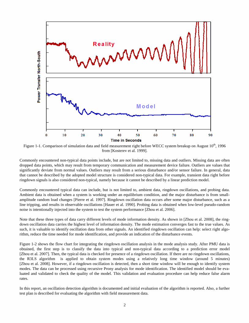
Figure 1-1. Comparison of simulation data and field measurement right before WECC system breakup on August 10th

, 1996

from [Kosterev et al. 1999]. ........................................................................................................................... 2

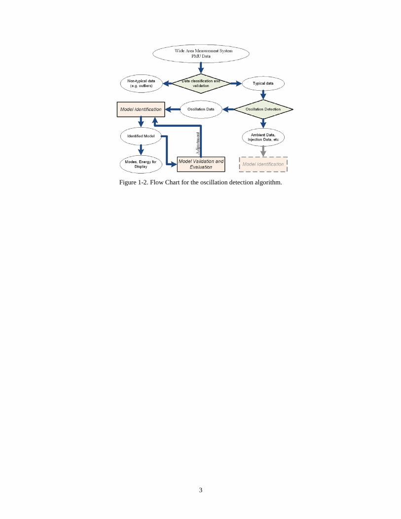
Figure 1-2. Flow Chart for the oscillation detection algorithm. ....................................................................................................... 3

Figure 4-1. One-line diagram of 17-machine model system .......................................................................................................... 11

Figure 4-2. Different signal to noise ratio measurements for sample output of 17-machine system ............................................. 12

Figure 4-3. Example analysis intervals .......................................................................................................................................... 13

Figure 4-4. Algorithm SNR estimates for 17th order and 20 dB event SNR ................................................................................. 14

Figure 4-5. Mean detection point and standard deviations of detection for 400 Monte-Carlo trials of 17th order/length and 20 dB event SNR .................................................................................................................................................... 14

Figure 5-1. Annotated screenshot of initial GUI ............................................................................................................................ 16

Figure 5-2. Parameter configuration popup window ...................................................................................................................... 17

ix

Tables

Table 4-1. Percentage of Monte-Carlo trials successfully detected for varying signal to noise ratios and model orders .............. 12

Table 4-2. Event SNR simulations’ mean and standard deviation values ...................................................................................... 14

Table 4-3. Average SNR simulations’ mean and standard deviation value ................................................................................... 15

1

1.0 INTRODUCTION Small signal stability problems on the power grid can cause significant electromechanical oscillations, which may cause prob-lems if they are not properly addressed—leading to grid reliability issues and potentially large-scale blackouts. One example is the Western Interconnection system breakup that occurred on August 10, 1996 [Kosterev et al. 1999]. The breakup led to 30 GW in lost load. Over the course of the event, about 8 million customers and 24 million people were influenced [Pal 2005]. Other past significant events include, but are not limited to [Pal et al. 2005]:

• Southern Brazil (1970-1980, 1984) • Ghana-Ivory Coast (1985) • Taiwan (1985) • Western Australia (1982, 1983) • Scotland-England (1978) • South East Australia (1975) • Min-continent area power pool (1971, 1972) • Western Electric Coordinating Council (1964, 1996) • Italy-Yugoslavia-Austria (1971-1974) • Saskatchewan-Manitoba Hydro-Western Ontario (1996) • Detroit Edison (DE-Ontario Hydro – Hydro Quebec) (1960s, 1985).

To avoid system breakups caused by oscillations, the dynamic stability margin has to be established, which puts limits on the power transfer capacities. Accurate and timely information about the oscillations can help optimize these margin settings so that a grid can be operated at its full capacity while staying within the stability boundary. To provide timely information about grid oscillation, extensive studies have been carried out to identify power system modes. Modes are the eigenvalues of linearized power system models. Generally, there are two basic approaches for estimating power system modes: component-based methods and measurement-based methods. With the component-based method, the nonlinear differential equations governing the system are linearized around an operating point. The power system modes are then obtained through eigenvalue analysis [Chow 1997]. On the other hand, for a measurement-based method, a linear model is estimated from direct system measurements. An important aspect to remember is that for a large complex power system, the efforts of building a component-based model are not trivial. For example, an initial effort was made by [Kosterev et al. 1999] to build a component-based model for simulating the Western Electricity Coordinating Council (WECC) reaction right before the breakup of August 10, 1996. Figure 1-1 shows that the simulation data did not match the field measurement data. The matched simulation and measurement was only achieved after extensive studies. In contrast, measurement-based approach usually requires significantly less effort than that required for a model-based method. The measurement-based method can update the mode estimation based on incoming measurement data. Thus, the measurement-based methods serve as a good complement to model-based methods in monitoring power system modes in real time. There exist several measurement-based small signal stability analysis algorithms, which have been developed and studied [Liu et al. 2007] [Liu and Vekatasubramanian 2008][Hauer et al. 1990] [Pierre et al. 1997][Kamwa et al. 1996] [Messina et al. 2006][ Trudnowski et al. 2008][ Sanchez-Gasca et al. 1999] [Zhou et al. 2006, 2007, 2008, 2009]. Performance studies of the existing small signal stability analysis algorithms have been mostly carried out using simulated data from simpli-fied models. There are no comparisons of the algorithms using field measurement data. One reason for the lack of this compari-son is likely tied to algorithm performance and its likelihood to be situation-dependent. One algorithm would perform better under some circumstances, while others may perform better in other circumstances. Ultimately, it is conjectured that the right combination of algorithms needs to be used to support real-time power grid operation [Liu et al. 2007]. Applying a mode analy-sis algorithm on a data set that is not suitable for that particular algorithm may result into degraded performance, and even false or missing alarms. To achieve desired performance and reduce false/missing alarms, measurement data should be classified into different categories to be sure that a proper mode identification algorithm can be selected. In general, field measurement data can be classified into two categories: typical and non-typical data. Typical data is data that carries system mode information and can be described by the model structure used by an identification algorithm. In contrast, non-typical data does not carry information about system modes and cannot be described by a general linear model.

2

Figure 1-1. Comparison of simulation data and field measurement right before WECC system breakup on August 10th

, 1996 from [Kosterev et al. 1999].

Commonly encountered non-typical data points include, but are not limited to, missing data and outliers. Missing data are often dropped data points, which may result from temporary communication and measurement device failure. Outliers are values that significantly deviate from normal values. Outliers may result from a serious disturbance and/or sensor failure. In general, data that cannot be described by the adopted model structure is considered non-typical data. For example, transient data right before ringdown signals is also considered non-typical, namely because it cannot be described by a linear prediction model. Commonly encountered typical data can include, but is not limited to, ambient data, ringdown oscillations, and probing data. Ambient data is obtained when a system is working under an equilibrium condition, and the major disturbance is from small-amplitude random load changes [Pierre et al. 1997]. Ringdown oscillation data occurs after some major disturbance, such as a line tripping, and results in observable oscillations [Hauer et al. 1990]. Probing data is obtained when low-level pseudo-random noise is intentionally injected into the system to test the system performance [Zhou et al. 2006]. Note that these three types of data carry different levels of mode information density. As shown in [Zhou et al. 2008], the ring-down oscillation data carries the highest level of information density. The mode estimation converges fast to the true values. As such, it is valuable to identify oscillation data from other signals. An identified ringdown oscillation can help: select right algo-rithm, reduce the time needed for mode identification, and provide an indication of the disturbance events. Figure 1-2 shows the flow chart for integrating the ringdown oscillation analysis in the mode analysis study. After PMU data is obtained, the first step is to classify the data into typical and non-typical data according to a prediction error model [Zhou et al. 2007]. Then, the typical data is checked for presence of a ringdown oscillation. If there are no ringdown oscillations, the R3LS algorithm is applied to obtain system modes using a relatively long time window (around 5 minutes) [Zhou et al. 2008]. However, if a ringdown oscillation is detected, then a short time window will be enough to identify system modes. The data can be processed using recursive Prony analysis for mode identification. The identified model should be eva-luated and validated to check the quality of the model. This validation and evaluation procedure can help reduce false alarm rates. In this report, an oscillation detection algorithm is documented and initial evaluation of the algorithm is reported. Also, a further test plan is described for evaluating the algorithm with field measurement data.

3

Figure 1-2. Flow Chart for the oscillation detection algorithm.

4

2.0 BACKGROUND As mentioned in Section 1.0, grid oscillations are closely related to different modes of interest on the power system. If the entire power system were modeled as a transfer function, modes are represented by the denominator, or poles of the system. These modes are often the result of generator controls from a wide geographical distribution interacting. If these interactions become unstable, the generator pairs associated with this interaction will swing against one another in a stronger and stronger fashion until the system collapses, or suitable mitigation control is enacted. Because modes are represented by the poles of a system, it is also useful to think of them as the natural resonances in the system. The best example of system resonance is a piano tuning fork. When excited by an event (in this case, striking the tuning fork), the natural resonances of the system become apparent. In the case of the tuning fork, a distinct, decaying pitch can be heard as the system returns to its steady state. The power system is very similar in this respect. If excited by an event such as a line trip-ping, the system will resonate at these modal frequencies. If the system is stable, these oscillations will slowly damp and the system will return to an equilibrium condition. However, if the system is unstable, as it was in the WECC 1996 case presented in Figure 1-1, these oscillations will grow until corrected, or system damage occurs. Modes of oscillation typically have two parameters of interest. These parameters are the frequency and damping ratio of the mode. Keeping with the tuning fork example, the frequency of the mode is the particular pitch at which it resonates. The damp-ing ratio is a measure of how fast the tone will fade away if the tuning fork is no longer excited. If a mode has a sufficiently low damping ratio, subsequent excitations could push the system to a failure point, despite the overall conditions being “stable”. In terms of the power system, if an outage occurs to induce such a resonance on the electrical grid, operators need to quickly know the new conditions of the system. If the resultant transient will sustain itself, or if the system is closer to an unstable oper-ating point, remedial actions must be taken. For this reason, accurate estimation of power systems modes is desired. With knowledge of a growing instability or a change in stability margins, operators can adjust the power system to prevent complete failure of the system. In instances of line or generator outages, the system may not become unstable, but the knowledge of the new damping ratio and stability margin can easily influence subsequent actions or planned immediate switching conditions. Utilizing the oscillation detection algorithm presented, modal estimates from ringdown events can quickly be identified and es-timated, providing the necessary information to operators on a timeline faster than a longer, ambient data estimation method.

5

3.0 DESCRIPTION OF THE OSCILLATION DETECTION ALGORITHM To reduce the rates of false and missing alarm, it is important to make sure that the right algorithm is applied to a right data set. For example, when a ringdown oscillation is detected, a Prony analysis method can be applied [Hauer et al. 1990]. In this sec-tion, a method for identifying ringdown signal from measurement data is discussed.

1. A review on the Prony analysis. As discussed in [Hauer et al. 1990], Prony analysis can be used to determine the system modes from ringdown signal. If a sys-tem can be described by a linear state space model, the homogeneous responses of the system are a sum of exponentially damped sinusoidal signals. The response is called a ringdown signal and can be described by

( )∑=

=n

iii tcty

1exp)( λ ( 3-1)

where y(t) is the measurement data at time t. Here λ i stands for the ith eigenvalue, which is a complex number. ci stands for the amplitude of ith mode, which is a complex number. The symbol n is the total number of eigenvalues. At sample time tk

=k·Δt, a sample discrete ringdown signal y[k] can be described as

[ ] ( )tzzctyky ii

n

i

kiitkt

∆=== ∑=

∆=λexp where)(

1

( 3-2)

Here Δt is the sampling interval. To determine the λ i

, y[k] can be written in a matrix format as

⋅

=

−−−−

+++

−

−

−

−

−−−−−−01

02

122

01

111

11

121

111

2221

211

1121

111

0022

011

]1[]2[]1[

]2[]1[]2[]1[][]1[]0[]1[][

nnn

nn

nn

nn

nNn

nNnN

nn

nn

nn

zzz

zzzzzz

zczczc

zczczczczczczczczc

nNyNyNy

ynynyynynyynyny

( 3-3)

Note that the most right matrix about zi’s in (3-3) is a Vandermonde matrix. Thus, there exists a set of indexes aj

’s, which can be defined as

,,,2,1for 0022

11 nizazazaz in

ni

ni

ni ==++++ −− ( 3-4)

or in matrix form as

0

1

1

01

02

122

01

111

=

⋅

−

−

−

nnnn

nn

nn

nn

a

a

zzz

zzzzzz

( 3-5)

It can be derived from (3-3) and (3-5) that

=

⋅

−−−−

+++

−

0

0001

]1[]2[]1[

]2[]1[]2[]1[][]1[]0[]1[][

2

1

na

aa

nNyNyNy

ynynyynynyynyny

( 3-6)

6

−

++

−=

⋅

−−−−

+−−−

]1[

]2[]1[

][

]1[]3[]2[

]2[][]1[]1[]1[][]0[]2[]1[

3

2

1

Ny

nyny

ny

a

aaa

nNyNyNy

ynynyynynyynyny

n

( 3-7)

Note that only the measurements of y[k]’s can be obtained. In the measurement data ][ˆ ky , there are measurement noises and process noise besides the multiple exponential terms in (3-2). Thus, the equation holds for measurement data with a noise term:

−

++

+

−

++

−=

⋅

−−−−

+−−−

]1[

]2[]1[

][

]1[ˆ

]2[ˆ]1[ˆ

][ˆ

ˆ

ˆˆˆ

]1[ˆ]3[ˆ]2[ˆ

]2[ˆ][ˆ]1[ˆ]1[ˆ]1[ˆ][ˆ]0[ˆ]2[ˆ]1[ˆ

3

2

1

Ne

nene

ne

Ny

nyny

ny

a

aaa

nNyNyNy

ynynyynynyynyny

n

( 3-8)

To increase estimation accuracy, the number of the samples in the data, N, is usually chosen to be greater than 2*n to form a set of over-determined equations in (3-8). A least-squares (LS) algorithm is applied to solve the equations. Also, to suppress noise, the model order in equation (3-8) is usually chosen to be higher than the number damped sinusoidal signals. The aj’s can be found by solving (3-7) in the least-squares sense. The estimates of zi iz, denoted as , can be estimated as the roots of the polynomial of

0ˆˆˆˆˆˆˆ 02

21

1 =++++ −− zazazaz nnnn ( 3-9)

According to [Pierre et al. 1997], the eigenvalues, or the modes, of the system can be estimated as

)ˆln(1ˆii z

t∆=λ ( 3-10)

The frequency and damping ratio of the modes can be calculated as

( ))(cos ii angleDR λ−=∆

( 3-11)

πλ

2)( i

iimagFreq

∆

= ( 3-12)

2. Application of the Prony method on the ringdown signal identification Once the eigenvalues λ i and zi are identified, the time domain ringdown signal can be reconstructed using the following proce-dure. According to equation (3-3), the following equation can be used to estimate oscillation amplitude ci ic denoted as :

−

=

⋅

−−−− ]1[

]1[]0[

ˆ

ˆˆ

ˆˆˆ

ˆˆˆˆˆˆ

2

1

1112

11

112

11

002

01

Ny

yy

c

cc

zzz

zzzzzz

nnN

nNN

n

n

( 3-13)

Note that the equation (3-13) is an over-determined equation. A LS algorithm can now be applied to estimate ic . The

time do-main ringdown signal can be reconstructed as

7

⋅

=

− −−−−n

nNn

NN

n

n

c

cc

zzz

zzzzzz

Ny

yy

ˆ

ˆˆ

ˆˆˆ

ˆˆˆˆˆˆ

]1[ˆ

]1[ˆ]0[ˆ

2

1

1112

11

112

11

002

01

( 3-14)

Note that the reconstructed ringdown signal [ ]ky usually does not match the measurement [ ]ky exactly. The signal-noise ratio can be applied to check the fit of the two signals. With the reconstructed ringdown signal, there are two metrics that can be applied to check the validity of the ringdown assump-tion, signal noise ratio, and stationary noise assumption. Define the estimated noise as

[ ] [ ] [ ]kykyke ˆˆ −= ( 3-15)

The signal-to-noise ratio (SNR) is then defined as

[ ]

[ ]∑

∑−

=

−

== 1

0

2

1

0

2

ˆ

ˆSNR N

i

N

i

ke

ky ( 3-16)

A large SNR indicates that a good fit is achieved and the ringdown assumption may hold. On the other hand, a small SNR indi-cates that the fit is not good and the ringdown assumption may not hold.

3. A block implementation for the oscillation detection algorithm. As discussed in [Zhou et al. 2007] and [Pierre and Zhou 2007], a robust and recursive implementation can help improve the im-plementation efficiency and robustness against outliers. To implement the proposed oscillation algorithm recursively and robust-ly, the following procedure is implemented. To simplify the notation, equation (3-8) can be written in a matrix format as

][][][][ kekkHky

+= θ ( 3-17)

where k is the starting time when the Prony analysis can be applied.

−+

+++

=

]1[ˆ

]1[ˆ][ˆ

][

Nky

nkynky

ky

( 3-18)

=

na

aaa

k

ˆ

ˆˆˆ

][ 3

2

1

θ

( 3-19)

−+

++++

+

=

]1[

]2[]1[

][

][

Nke

nkenke

nke

ke

( 3-20)

8

−+

+−+

=

]2[

][]1[

][

Nk

nknk

kH

T

T

T

ϕ

ϕϕ

( 3-21)

+−

−=

]1[ˆ

]1[ˆ][ˆ

][ where

niy

iyiy

i

ϕ ( 3-22)

Note that here n is the order of Prony model, and N-n is the number of equations. Thus, an objective function of the least-square solution can be described as

( ) 0][][1

21 ≥⋅= ∑−+

+=

−−+ kforiekJNk

nki

iNkλθ ( 3-23)

where λ is the forgetting factor, which is a positive number slightly smaller or equal to 1.

Writing the above objective function in matrix format, we have

( ) ( ) ( ) 0for ][][][][][][][][][][1

21 ≥−Λ−=Λ=⋅= ∑−+

+=

−−+ kkkHkykkHkyieieiekJ TTNk

nki

iNk θθλθ ( 3-24)

where

=Λ−

−−

0

2

1

λ

λλ

L

nN

( 3-25)

is a diagonal matrix. Thus , the least-square solution can be defined as

( ){ }][minarg][ˆ][

kJkk

θθθ

= ( 3-26)

The least square solution can be found by setting the derivative of the objective function to 0 as following

( ) [ ] 0][][ˆ][][][ˆ][ˆ setT

kHkkHkykkJ

=Λ⋅−−=∂∂ θθθ ( 3-27)

Thus, the block solution can be derived as

[ ]( )

( ) ( )][][][ˆ

][][][][][ˆ

][][][ˆ][][

0][ˆ][][][

1

1

kskk

kykHkHkHk

kykHkkHkH

kkHkykH

TT

TT

T

⋅Φ=⇒

ΛΛ=⇒

Λ=Λ⇒

=⋅−Λ−⇒

−

−

θ

θ

θ

θ

( 3-28)

where

9

][][][ kHkHk T Λ=Φ∆

( 3-29)

][][][ kykHks T Λ=

∆ ( 3-30)

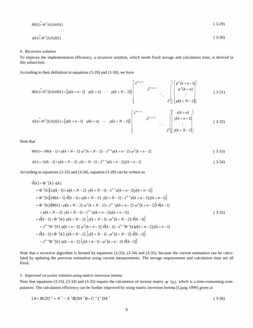
4. Recursive solution To improve the implementation efficiency, a recursive solution, which needs fixed storage and calculation time, is derived in this subsection. According to their definition in equations (3-29) and (3-30), we have

[ ]

−+

+−+

⋅

⋅−++−+=Λ=Φ−−

−−

∆

]2[

][]1[

]2[][]1[][][][

0

2

1

Nk

nknk

NknknkkHkHkT

T

nN

nN

T

ϕ

ϕϕ

λ

λλ

ϕϕϕ

( 3-31)

[ ]

−+

+++

⋅−++−+=Λ=−−

−−

∆

]1[

]1[][

]2[][]1[][][][

0

2

1

Nky

nkynky

NknknkkykHksnN

nN

T

λ

λλ

ϕϕϕ

( 3-32)

Note that

]2[]2[]2[]2[]1[][ −+⋅−+−−+⋅−++−Φ=Φ − nknkNkNkkk TnNT ϕϕλϕϕλ ( 3-33)

]1[]2[]1[]2[]1[][ −+−+−−+⋅−++−= − nkynkNkyNkksks nN ϕλϕλ ( 3-34)

According to equations (3-33) and (3-34), equation (3-28) can be written as

{ }{ }( )

{ }

{ }( )]1[ˆ]2[]1[]2[][

]1[ˆ]2[]1[]2[][]1[ˆ]1[]2[][]1[ˆ]2[]2[][

]1[ˆ]2[]1[]2[][]1[ˆ]}1[]2[]1[]2[

]1[ˆ]2[]2[]2[]2[][]{[

]1[]2[]1[]2[]1[ˆ]1[][

]1[]2[]1[]2[]1[][

][][][ˆ

1

1

11

1

1

1

1

1

−⋅−+−−+⋅−+⋅Φ−

−⋅−+−−+⋅−+⋅Φ+−=

−+−+Φ−−⋅−+⋅−+⋅Φ+

−⋅−+−−+⋅−+⋅Φ+−=

−+−+−−+⋅−++

−⋅−+⋅−++−+⋅−+−ΦΦ=

−+−+−−+⋅−++−⋅−ΦΦ=

−+−+−−+⋅−++−Φ=

⋅Φ=

−−

−

−−−−

−

−

−−

−−

−−

−

knknkynkk

kNkNkyNkkk

nkynkkknknkk

kNkNkyNkkk

nkynkNkyNk

knknkNkNkkk

nkynkNkyNkkkk

nkynkNkyNkksk

kskk

TnN

T

nNTnN

T

nN

TnNT

nN

nN

θϕϕλ

θϕϕθ

ϕλθϕϕλ

θϕϕθ

ϕλϕ

θϕϕλϕϕ

ϕλϕθλ

ϕλϕλ

θ

( 3-35)

Note that a recursive algorithm is formed by equations (3-33), (3-34) and (3-35), because the current estimation can be calcu-lated by updating the previous estimation using current measurements. The storage requirements and calculation time are all fixed.

5. Improved recursive solution using matrix inversion lemma Note that equations (3-33), (3-34) and (3-35) require the calculation of inverse matrix ][1 k−Φ , which is a time-consuming com-putation. The calculation efficiency can be further improved by using matrix inversion lemma [Ljung 1999] given as

1111111 ][][ −−−−−−− +−=+ DACBDABAABCDA ( 3-36)

10

to circumvent the matrix inverse calculation. To facilitate notation, define:

kiiiP ,,1,0for ][][ 1 =Φ= −∆

( 3-37) Based on this choice, equation (3-28) can be written as

{ }

( )]1[ˆ]2[]1[]2[][

]1[ˆ]2[]1[]2[][]1[ˆ][ˆ

−⋅−+−−+⋅−+⋅−

−⋅−+−−+⋅−+⋅+−=− knknkynkkP

kNkNkyNkkPkkTnN

T

θϕϕλ

θϕϕθθ ( 3-38)

According equation (3-37), we have

{ } 11 ]2[]2[]2[]2[]1[][][ −−− −+⋅−+−−+⋅−++−Φ=Φ= nknkNkNkkkkP TnNT ϕϕλϕϕλ ( 3-39) Now, apply the matrix inversion lemma 2 times. 1) Matrix inversion lemma #1

{ } 11 ]2[]2[]2[]2[]1[][][ −−− −+⋅−++−+⋅−+−−Φ=Φ= NkNknknkkkkP TTnN ϕϕϕϕλλ

( 3-40)

( )( ) ( )

( ) ]2[]2[]2[]1[]2[1]2[]2[]1[]2[]2[]2[]2[]1[

]2[]2[]1[

1

11

1

−+−+⋅−+−−Φ−++

−+⋅−+−−Φ−+⋅−+−+⋅−+−−Φ−

−+⋅−+−−Φ=

−−

−−−−

−−

NknknkkNknknkkNkNknknkk

nknkk

TnNT

TnNTTnN

TnNlemmainversionmatrix

ϕϕϕλλϕϕϕλλϕϕϕϕλλ

ϕϕλλ

Define

( ) 1]2[]2[]1[][ −−∆

−+⋅−+−−Φ= nknkkkQ TnN ϕϕλλ ( 3-41) Then

]2[][]2[1][]2[]2[][][][

−+−++−+⋅−+

−=NkkQNk

kQNkNkkQkQkP T

T

ϕϕϕϕ ( 3-42)

2) Matrix inversion lemma #2

( ) 1]2[]2[]1[][ −−∆

−+⋅−+−−Φ= nknkkkQ TnN ϕϕλλ

( ) ( ) ( )( )

]2[]1[]2[]1[]2[]2[]1[]1[1

]2[]1[]2[1]1[]2[]2[]1[]1[

1

1

111

−+−−++−−+−+−

−−=

−+−Φ−++⋅−Φ−+−+−Φ

−−Φ=

−+−

−−

−−−−

nkkPnkkPnknkkPkP

nkknkknknkkk

TnN

T

nNT

nNTlemmainversionmatrix

ϕϕλϕϕ

λ

λϕλϕλλϕϕλλ

( 3-43)

At each new time step, k, use (3-43) to calculate Q[k], use (3-42) to calculate P[k], and use (3-38) to calculate ][ˆ kθ .

11

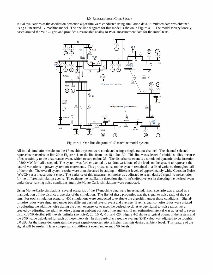
4.0 RESULTS FROM CASE STUDY Initial evaluations of the oscillation detection algorithm were conducted using simulation data. Simulated data was obtained using a linearized 17-machine model. The one-line diagram for this model is shown in Figure 4-1. The model is very loosely based around the WECC grid and provides a reasonable analog to PMU measurement data for the initial tests.

Figure 4-1. One-line diagram of 17-machine model system

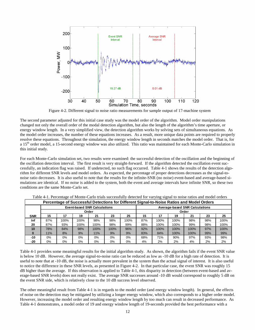
All initial simulation results on the 17-machine system were conducted using a single output channel. The channel selected represents transmission line 20 in Figure 4-1, or the line from bus 18 to bus 30. This line was selected for initial studies because of its proximity to the disturbance event, which occurs on bus 35. The disturbance event is a simulated dynamic-brake insertion of 800 MW for half a second. The system was further excited by random variations of the loads on the system to represent the natural variations in power system measurements. This process noise on the system remained at a fixed variance throughout all of the trials. The overall system results were then obscured by adding in different levels of approximately white Gaussian Noise (AWGN) as a measurement error. The variance of this measurement noise was adjusted to reach desired signal-to-noise ratios for the different simulation events. To evaluate the oscillation detection algorithm’s effectiveness in detecting the desired event under these varying noise conditions, multiple Monte-Carlo simulations were conducted. Using Monte-Carlo simulations, several scenarios of the 17-machine data were investigated. Each scenario was created as a manipulation of two distinct properties of the simulation. The first of these properties was the signal to noise ratio of the sys-tem. For each simulation scenario, 400 simulations were conducted to evaluate the algorithm under those conditions. Signal-to-noise ratios were simulated under two different desired levels: event and average. Event signal-to-noise ratios were created by adjusting the additive noise during the event occurrence to meet the desired level. Average signal-to-noise ratios were created by adjusting the additive noise during an ambient portion of the analysis. Each estimation interval was adjusted to seven distinct SNR decibel (dB) levels: infinite (no noise), 20, 10, 0, -10, and -20. Figure 4-2 shows a typical output of the system and the SNR value calculated for each of these intervals. In this particular case, the average SNR value was adjusted to be roughly 0.0 dB. As the figure demonstrates, the event signal-to-noise ratio is higher than this desired ambient level. This feature of the signal will be useful in later comparisons of different event and event SNR levels.

12

Figure 4-2. Different signal to noise ratio measurements for sample output of 17-machine system

The second parameter adjusted for this initial case study was the model order of the algorithm. Model order manipulations changed not only the overall order of the modal detection algorithm, but also the length of the algorithm’s time aperture, or energy window length. In a very simplified view, the detection algorithm works by solving sets of simultaneous equations. As the model order increases, the number of these equations increases. As a result, more unique data points are required to properly resolve these equations. Throughout the simulation, the energy window length in seconds matches the model order. That is, for a 15th

order model, a 15-second energy window was also utilized. This ratio was maintained for each Monte-Carlo simulation in this initial study.

For each Monte-Carlo simulation set, two results were examined: the successful detection of the oscillation and the beginning of the oscillation detection interval. The first result is very straight-forward. If the algorithm detected the oscillation event suc-cessfully, an indication flag was raised. If undetected, no such flag occurred. Table 4-1 shows the results of the detection algo-rithm for different SNR levels and model orders. As expected, the percentage of proper detections decreases as the signal-to-noise ratio decreases. It is also useful to note that the results for the infinite-SNR (no noise) event-based and average-based si-mulations are identical. If no noise is added to the system, both the event and average intervals have infinite SNR, so these two conditions are the same Monte-Carlo set.

Table 4-1. Percentage of Monte-Carlo trials successfully detected for varying signal to noise ratios and model orders

Table 4-1 provides some meaningful results for the initial algorithm study. As shown, the algorithm fails if the event SNR value is below 10 dB. However, the average signal-to-noise ratio can be reduced as low as -10 dB for a high rate of detection. It is useful to note that at -10 dB, the noise is actually more prevalent in the system than the actual signal of interest. It is also useful to notice the difference in these SNR levels, as presented in Figure 4-2. In that particular case, the event SNR was roughly 15 dB higher than the average. If this observation is applied to Table 4-1, this disparity in detection (between event-based and av-erage-based SNR levels) does not really exist. The average SNR successes around -10 dB would correspond to roughly 5 dB on the event SNR side, which is relatively close to the 10 dB success level observed. The other meaningful result from Table 4-1 is in regards to the model order (and energy window length). In general, the effects of noise on the detection may be mitigated by utilizing a longer energy window, which also corresponds to a higher order model. However, increasing the model order and resulting energy window length by too much can result in decreased performance. As Table 4-1 demonstrates, a model order of 19 and energy window length of 19-seconds provided the best performance with a

15 17 19 21 23 25 15 17 19 21 23 25Inf 87% 100% 100% 98% 98% 100% 87% 100% 100% 98% 98% 100%20 87% 93% 100% 100% 98% 99% 88% 100% 100% 99% 98% 100%10 78% 84% 98% 100% 100% 96% 92% 100% 100% 100% 97% 100%0 11% 8% 9% 11% 9% 9% 83% 84% 100% 100% 99% 99%

-10 0% 0% 0% 0% 0% 0% 68% 71% 90% 97% 93% 98%-20 0% 0% 0% 0% 0% 0% 4% 2% 2% 4% 2% 2%

Percentage of Successful Detections for Different Signal-to-Noise Ratios and Model Orders

SNROrder

Average-based SNR CalculationsEvent-based SNR CalculationsOrder

13

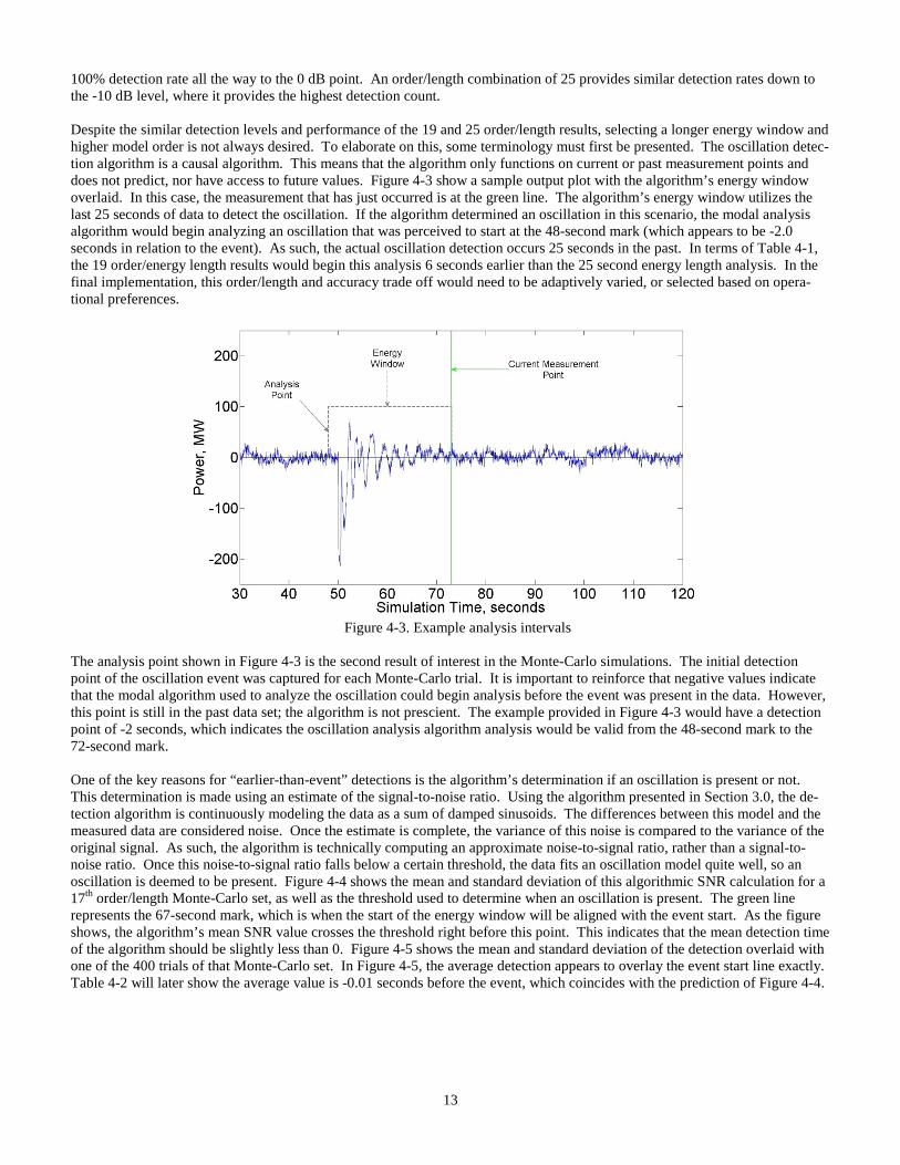
100% detection rate all the way to the 0 dB point. An order/length combination of 25 provides similar detection rates down to the -10 dB level, where it provides the highest detection count. Despite the similar detection levels and performance of the 19 and 25 order/length results, selecting a longer energy window and higher model order is not always desired. To elaborate on this, some terminology must first be presented. The oscillation detec-tion algorithm is a causal algorithm. This means that the algorithm only functions on current or past measurement points and does not predict, nor have access to future values. Figure 4-3 show a sample output plot with the algorithm’s energy window overlaid. In this case, the measurement that has just occurred is at the green line. The algorithm’s energy window utilizes the last 25 seconds of data to detect the oscillation. If the algorithm determined an oscillation in this scenario, the modal analysis algorithm would begin analyzing an oscillation that was perceived to start at the 48-second mark (which appears to be -2.0 seconds in relation to the event). As such, the actual oscillation detection occurs 25 seconds in the past. In terms of Table 4-1, the 19 order/energy length results would begin this analysis 6 seconds earlier than the 25 second energy length analysis. In the final implementation, this order/length and accuracy trade off would need to be adaptively varied, or selected based on opera-tional preferences.

Figure 4-3. Example analysis intervals

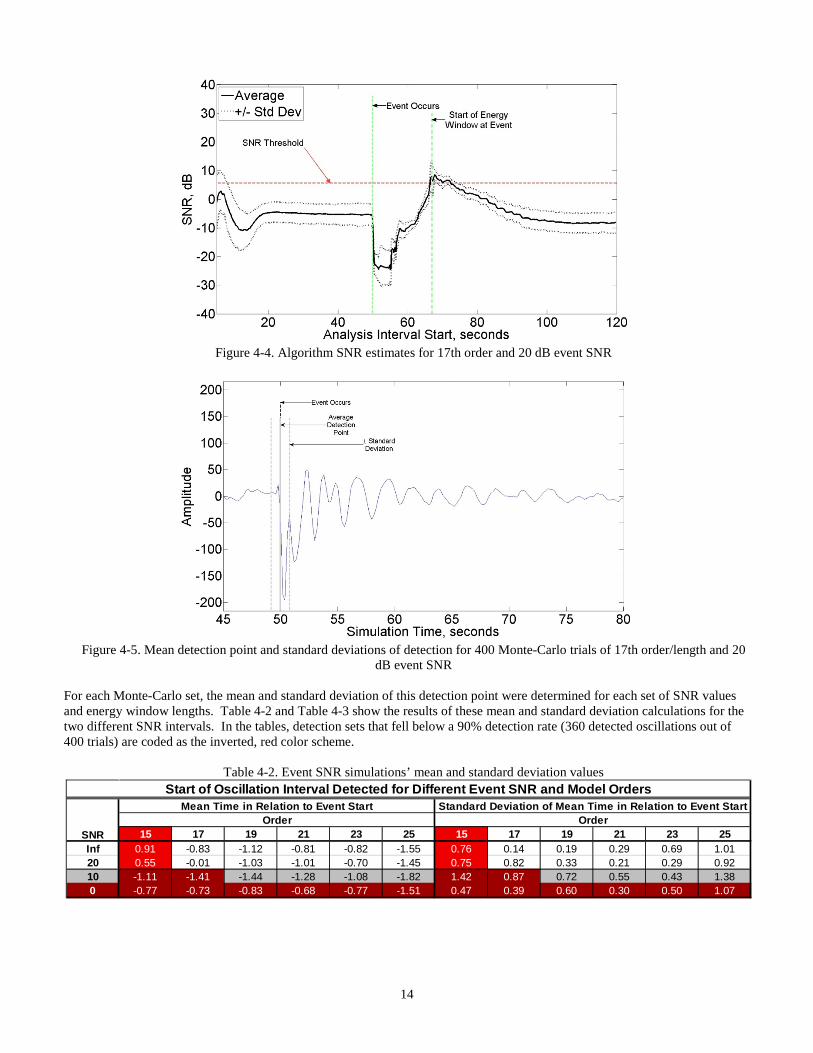
The analysis point shown in Figure 4-3 is the second result of interest in the Monte-Carlo simulations. The initial detection point of the oscillation event was captured for each Monte-Carlo trial. It is important to reinforce that negative values indicate that the modal algorithm used to analyze the oscillation could begin analysis before the event was present in the data. However, this point is still in the past data set; the algorithm is not prescient. The example provided in Figure 4-3 would have a detection point of -2 seconds, which indicates the oscillation analysis algorithm analysis would be valid from the 48-second mark to the 72-second mark. One of the key reasons for “earlier-than-event” detections is the algorithm’s determination if an oscillation is present or not. This determination is made using an estimate of the signal-to-noise ratio. Using the algorithm presented in Section 3.0, the de-tection algorithm is continuously modeling the data as a sum of damped sinusoids. The differences between this model and the measured data are considered noise. Once the estimate is complete, the variance of this noise is compared to the variance of the original signal. As such, the algorithm is technically computing an approximate noise-to-signal ratio, rather than a signal-to-noise ratio. Once this noise-to-signal ratio falls below a certain threshold, the data fits an oscillation model quite well, so an oscillation is deemed to be present. Figure 4-4 shows the mean and standard deviation of this algorithmic SNR calculation for a 17th

Figure 4-5

order/length Monte-Carlo set, as well as the threshold used to determine when an oscillation is present. The green line represents the 67-second mark, which is when the start of the energy window will be aligned with the event start. As the figure shows, the algorithm’s mean SNR value crosses the threshold right before this point. This indicates that the mean detection time of the algorithm should be slightly less than 0. shows the mean and standard deviation of the detection overlaid with one of the 400 trials of that Monte-Carlo set. In Figure 4-5, the average detection appears to overlay the event start line exactly. Table 4-2 will later show the average value is -0.01 seconds before the event, which coincides with the prediction of Figure 4-4.

14

Figure 4-4. Algorithm SNR estimates for 17th order and 20 dB event SNR

Figure 4-5. Mean detection point and standard deviations of detection for 400 Monte-Carlo trials of 17th order/length and 20

dB event SNR

For each Monte-Carlo set, the mean and standard deviation of this detection point were determined for each set of SNR values and energy window lengths. Table 4-2 and Table 4-3 show the results of these mean and standard deviation calculations for the two different SNR intervals. In the tables, detection sets that fell below a 90% detection rate (360 detected oscillations out of 400 trials) are coded as the inverted, red color scheme.

Table 4-2. Event SNR simulations’ mean and standard deviation values

15 17 19 21 23 25 15 17 19 21 23 25Inf 0.91 -0.83 -1.12 -0.81 -0.82 -1.55 0.76 0.14 0.19 0.29 0.69 1.0120 0.55 -0.01 -1.03 -1.01 -0.70 -1.45 0.75 0.82 0.33 0.21 0.29 0.9210 -1.11 -1.41 -1.44 -1.28 -1.08 -1.82 1.42 0.87 0.72 0.55 0.43 1.380 -0.77 -0.73 -0.83 -0.68 -0.77 -1.51 0.47 0.39 0.60 0.30 0.50 1.07

Start of Oscillation Interval Detected for Different Event SNR and Model Orders

SNROrder

Standard Deviation of Mean Time in Relation to Event StartMean Time in Relation to Event StartOrder

15

Table 4-3. Average SNR simulations’ mean and standard deviation value

As Table 4-2 and Table 4-3 demonstrate, for cases when the oscillation was detected 90% of the time or greater, the average detection time was typically within 1 second of the event’s presence in the data. Under these same circumstances, the standard deviation on the detection was typically less than 1 second. Recall from earlier that the 19th and 25th

Table 4-2 order/length analysis pro-

vided very high detection rates of the oscillation. In the results presented in both and Table 4-3, the 19th order model has a lower standard deviation and closer mean detection time than the 25th

order estimate. While the results of both estimates are reasonable, the lower variation and “closer to actual” detection time provides greater confidence that the output of the oscil-lation analysis function is valid.

From the results presented, the oscillation detection algorithm performed very well for the 17-machine test case. The algorithm successfully detected an oscillatory event within a reasonable amount of time and within reasonable consistency. Under condi-tions around and below 0 dB SNR, at which point noise is equal to, or greater than the signal, the algorithm does begin to expe-rience decreased performance. However, in these cases the oscillation is nearly invisible in the measurement data. Furthermore, such conditions would likely be the indication of a much greater problem than an oscillatory event on the system. This case study also indicates variations of parameters (either expertly or through an adaptive algorithm) can lead to improve-ments and adjustments in this consistency. For identical SNR levels, adjusting the model order and energy window length of the algorithm often resulted in some improvement of the detection time and variance. It is important to point out that these results may be particular to the 17-machine model utilized. These results may be valid only for the particular configuration, or even the 800 MW disturbance event of this study. Different systems may exhibit better behavior for the 25th order/length case, rather than the 19th

order/length case. Further cases and studies are required to provide answers to these questions.

15 17 19 21 23 25 15 17 19 21 23 25Inf 0.91 -0.83 -1.12 -0.81 -0.82 -1.55 0.76 0.14 0.19 0.29 0.69 1.0120 0.80 -0.80 -1.09 -0.86 -0.75 -1.58 0.53 0.22 0.16 0.23 0.64 0.9710 0.68 -0.66 -1.04 -0.93 -0.65 -1.57 0.34 0.39 0.19 0.19 0.46 0.870 0.80 -0.02 -1.03 -1.07 -0.79 -1.43 1.40 0.96 0.43 0.26 0.30 1.00

-10 -1.30 -1.48 -1.53 -1.24 -1.02 -1.71 0.75 0.63 0.69 0.57 0.51 1.42-20 -0.53 -1.02 -0.76 -0.67 -0.83 -1.43 0.30 0.54 0.50 0.31 0.18 1.06

Start of Oscillation Interval Detected for Different Average SNR and Model Orders

SNROrder

Standard Deviation of Mean Time in Relation to Event StartMean Time in Relation to Event StartOrder

16

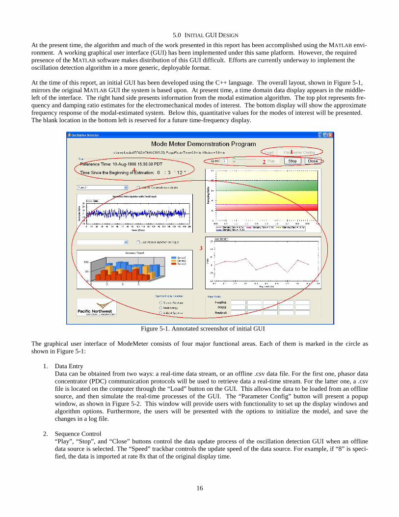
5.0 INITIAL GUI DESIGN At the present time, the algorithm and much of the work presented in this report has been accomplished using the MATLAB envi-ronment. A working graphical user interface (GUI) has been implemented under this same platform. However, the required presence of the MATLAB software makes distribution of this GUI difficult. Efforts are currently underway to implement the oscillation detection algorithm in a more generic, deployable format. At the time of this report, an initial GUI has been developed using the C++ language. The overall layout, shown in Figure 5-1, mirrors the original MATLAB GUI the system is based upon. At present time, a time domain data display appears in the middle-left of the interface. The right hand side presents information from the modal estimation algorithm. The top plot represents fre-quency and damping ratio estimates for the electromechanical modes of interest. The bottom display will show the approximate frequency response of the modal-estimated system. Below this, quantitative values for the modes of interest will be presented. The blank location in the bottom left is reserved for a future time-frequency display.

Figure 5-1. Annotated screenshot of initial GUI

The graphical user interface of ModeMeter consists of four major functional areas. Each of them is marked in the circle as shown in Figure 5-1:

1. Data Entry Data can be obtained from two ways: a real-time data stream, or an offline .csv data file. For the first one, phasor data concentrator (PDC) communication protocols will be used to retrieve data a real-time stream. For the latter one, a .csv file is located on the computer through the “Load” button on the GUI. This allows the data to be loaded from an offline source, and then simulate the real-time processes of the GUI. The “Parameter Config” button will present a popup window, as shown in Figure 5-2. This window will provide users with functionality to set up the display windows and algorithm options. Furthermore, the users will be presented with the options to initialize the model, and save the changes in a log file.

2. Sequence Control “Play”, “Stop”, and “Close” buttons control the data update process of the oscillation detection GUI when an offline data source is selected. The “Speed” trackbar controls the update speed of the data source. For example, if “8” is speci-fied, the data is imported at rate 8x that of the original display time.

17

3. Data Display

Data Display is composed of plotting displays and tabular array display. There are four plotting panels on the ModeMe-ter GUI, which perform a variety of tasks and draw different dynamic curves or plots upon received new data. The Ma-jor Modes tabular table shows the parameters of modes of interest, dynamically based on the results of the oscillation detection algorithm.

4. Time Display Time Display shows both the program’s overall running time, and the elapsed plotting time based on a particular source of data.

Figure 5-2. Parameter configuration popup window

At this stage in the development, the GUI is only partially functional. The ability to import data from saved .csv files has been implemented and tested. Work has begun on incorporating PDC streams into the GUI as a real-time data source. An FFT computation package has been selected, tested, and integrated into the GUI successfully. At this time, a crude version of the R3LS algorithm is implemented in the GUI and provides analysis results. Efforts are currently focusing on the full implementa-tion of this algorithm and the accompanying oscillation detection algorithm.

18

6.0 TEST PLAN To further test and improve the performance of the proposed algorithm, we propose that tests should be performed based on the field measurement PMU data from WECC system. The data should include normal operational data and special event data. The normal operational data is a data set of 24 hours from Malin-Round Mountain line in WECC system. First, the data set in *.dst format should be identified from the archived database available in the Electricity Infrastructure Operations Center (EIOC) of PNNL. Then, the DSItoolbox is to be used to extract the data from *.dst into *.mat file and/or *.txt file. Next, plots should be generated on 5-minute intervals. Oscillation events should first be manually identified through visual inspection on the 5-minute interval plots. Finally, the proposed algorithm is applied on the data set recursively to identify ringdown oscillation. The results from manual inspection and oscillation identification algorithms will be cross-checked to verify the results. The false alarm and missing alarm should be summarized to evaluate the performance of the proposed oscillation identification algorithm. Special event data sets are data recorded around some major disturbance events, such as generation trip, major transmission line trip, and oscillation events. First, major typical events in WECC are to be identified by consulting experts (e.g., Dr. John Hauer, Bill Mittelstadt). Then, the corresponding achived data files are to be identified from the PNNL EIOC database, or from posted WECC event data. These original data files are likely in the *.dst file format. Once again, the DSItoolbox is to be used to con-vert the data from *.dst to *.mat file and/or *.txt file. The proposed algorithm is to be applied for detecting ringdown oscillation events. The results from manual inspection and oscillation identification algorithms will again be cross-checked to verify the results. During the application of the oscillation detection algorithm, the modes are going to be identified. For some events, the modes have been manually calculated using block algorithms. These study results are going to be compared with the proposed algorithm. Finally, an evaluation report is going to be prepared for the evaluation study.

19

7.0 CONCLUSIONS This report proposed an oscillation detection algorithm for speeding up mode identification of a power system based on PMU data. Modal analysis provides vital information about the power system stability. On-line mode identification algorithms based on PMU measurements provide a way for monitoring power system modes in real time. Oscillation alarms can be issued when the power system is lightly damped. A good oscillation alarm tool (a.k.a. ModeMeter) can provide time for operators to take remedial reaction and reduce the probability of a system breakup as a result of such a light damping condition. The applicability of the mode identification algorithms relies heavily on the proper use of algorithms. Identification algorithms can provide dependable mode information only when they are applied properly on the right signal types. Improper application of algorithms may result in false alarm and/or missing alarm. One of most import categories of data is the oscillation ringdown data, which results from major disturbances. It is important to detect the oscillation ringdown to properly apply Prony’s method to promptly identify modes within a short time window. In this report, an oscillation detection algorithm is proposed for on-line identification of the ringdown data. Assumption verification is used to check occurrence of ringdown data. The basic assumption of ringdown signal is that the signal is consisted of multiple damped sinusoidal signals. By applying the Prony analysis, the original signal can be decomposed into the damped sinusoidal signals and noise. To verify the multiple damped sinusoid assumption, a signal-to-noise ratio is calculated. A higher SNR indicates a higher probability that the assump-tion, that an oscillation is present, holds. While a lower SNR indicates a lower probability that the assumption holds. To make the algorithm work on-line, a recursive algorithm is developed for high implementation efficiency. Initial simulation shows that the proposed method can work efficiently to identify the proper data set to apply Prony analysis. Thus, the mode identification procedure can be speed up with reduced window size for the ringdown data. Also, it reduces the rate of false alarm and missing alarm. Furthermore, a study plan on field measurement PMU data is also described.

20

8.0 BIBLIOGRAPHY [1] Pal, B. and B. Chaudhuri, Robust Control in Power Systems, Springer US, 2005 [2] Chow, J., Power System Toolbox, Dynamic Tutorial and Functions, 1997. [3] Kosterev, D. N., C. W. Taylor, and W. A. Mittelstadt, “Model Validation for the August 10, 1996 WSCC System Outage,” IEEE Transactions on Power

Systems, vol. 14, no. 3, pp. 967-979, August 1999. [4] Liu, G., J. Quintero, and V. Venkatasubramanian, “Oscillation Monitoring System based on wide area synchrophasors in power systems,” Proc. IREP

symposium 2007. Bulk Power System Dynamics and Control - VII, August 19-24, 2007, Charleston, South Carolina, USA. [5] Liu G., and V. Venkatasubramanian, "Oscillation monitoring from ambient PMU measurements by Frequency Domain Decomposition," Proc. IEEE Inter-

national Symposium on Circuits and Systems, Seattle, WA, May 2008, pp. 2821-2824. [6] Ljung, L., System Identification: Theory for the User, 2nd

[7] Hauer, J.F., C. J. Demeure, and L.L. Scharf, “Initial Results in Prony Analysis of Power System Response Signals,” IEEE Transactions on Power Systems, vol. 5, no. 1, pp. 80-89, Feb. 1990.

edition, Prentice Hall, Upper Saddle River, New Jersey, 1999.

[8] Pierre, John and Ning Zhou, "R3LS with Finite Duration Exponential Window," worknotes, Dec. 2007. [9] Pierre, J.W., D.J. Trudnowski, and M. K. Donnelly , “Initial results in electromechanical mode identification from ambient data,” IEEE Transactions on

Power Systems, vol.12, no.3, pp. 1245-1251, Aug. 1997. [10] Kamwa, I., G. Trudel, and L. Gerin-Lajoie, "Low-order Black-box Models for Control System Design in Large Power Systems

[11] Messina, A. and Vijay Vittal, “Nonlinear, non-stationary analysis of interarea oscillations via Hilbert spectral analysis,” IEEE Transactions on Power Systems, vol. 21, no 3, pp. 1234-1241, Aug, 2006.

," IEEE Transactions on Power Systems, vol. 11, no. 1, pp. 303-311. Feb. 1996

[12] Trudnowski, D., J. Pierre, N. Zhou, J. Hauer, and M. Parashar, “Performance of Three Mode-Meter Block-Processing Algorithms for Automated Dynamic Stability Assessment,” IEEE Transactions on Power Systems, vol. 23, no. 2, pp. 680-690, May 2008.

[13] Sanchez-Gasca, J. J., and J. H. Chow, “Performance Comparison of Three Identification Methods for the Analysis of Electromechanical Oscillations”, IEEE Transactions on Power Systems, vol. 14, no. 3, pp. 995-1001. Aug. 1999.

[14] Zhou, N., J. Pierre, and J. Hauer, “Initial Results in Power System Identification from Injected Probing Signals Using a Subspace Method,” IEEE Transac-tion on Power Systems, vol. 21, no. 3, pp. 1296-1302, Aug 2006.

[15] Zhou, N., J. Pierre, D. Trudnowski, and R. Guttromson, “Robust RLS Methods for On-line Estimation of Power System Electromechanical Modes,” IEEE Transactions on Power Systems, vol. 22, no. 3, Aug. 2007, pp. 1240-1249.

[16] Zhou, N., D. Trudnowski, J. Pierre, and W. Mittelstadt, “Electromechanical Mode On-Line Estimation using Regularized Robust RLS Methods”, EEE Transactions on Power Systems, vol. 24, no. 4, pp. 1670-1680, November 2008

[17] Zhou, N., D. Trudnowski, and J. Pierre, “Mode Initialization for On-Line Estimation of Power System Electromechanical Modes,” Proceedings of the 2009 Power Systems Conference and Exposition (PSCE), Seattle, WA, March 15-19, 2009.