OPTIONS FOR IMPROVING IRRIGATION WATER ALLOCATION AND USE: A CASE STUDY IN HARI ROD RIVER BASIN,

AFGHANISTAN

by

Ahmad Faisal Basiri

A thesis submitted in partial fulfillment of the requirements for the Degree of Master of Engineering in

Water Engineering and Management

Examination Committee: Dr. Sylvain Perret (Chairperson) Dr. Mukand S. Babel Dr. Roberto S Clemente Dr. S Ranamukhaarachchi Nationality: Afghan Previous Degree: Bachelor of Science in Civil Engineering Herat University, Civil Engineering Faculty

Scholarship Donor: Norwegian Government

Asian Institute of Technology School of Engineering and Technology

Thailand May 2009

ii

ACKNOWLEDGEMENTS

First and foremost I offer my sincerest gratitude to my supervisor, Dr. Sylvian Perret, who has supported me throughout my thesis with his patience and knowledge whilst allowing me the room to work in my own way. I attribute the level of my Masters degree to his encouragement and effort and without him this thesis, too, would not have been completed or written. I would also like to express sincere gratitude to honorable committee members, Dr. Mukand S. Babel, Dr. Roberto S. Clemente, and Dr. S Ranamukhaarachachi for their thoughtful and constructive suggestions during the study. I acknowledge PMU director Eng. M. Gul and Eng. Bashir Ahmad for their co-operation and help during my data collection for my study. Besides, I would like to express profound gratitude to my classmates and friends who have helped me during my studies. Further thanks should also go to Eng. Sayed Sharif Shobair for recommending me to study at AIT. I wish to extend my deepest sense of gratitude to my beloved parents for their un-ending love, inspiration and blessing to achieve this height of my career. Appreciating this, I would like to dedicate this Master Thesis to my parents. Finally, a big thank you goes to the Royal Norwegian Government for providing the financial support to complete my studies at Asian Institute of Technology. In addition many thanks must go to the CIRAD-France for providing research support fund which was extremely helpful for completion of this research work.

iii

ABSTRACT

This study investigates cropping system options in context of irrigation water scarcity. It aims at improving irrigation water allocation with the objectives of maximizing net economic return and calories production, and minimizing selected production factors. CWR and IWR for all practiced crops are estimated for the case study area based on local climatic and cropping system information. Current field situation, as per farmers’ practices and water availability, is quantified in terms of demand and supply, and compared with the actual crop water needs. Different scenarios are tested including different possible cropping systems under optimal and sub-optimal water supply. CROPWAT model was used for calculating CWR, IWR, and for developing irrigation scheduling, to quantify the yield reduction for the practiced crops during water shortages time. The gross irrigation requirement is calculated on the basis of different irrigation efficiencies with 10-day time step in the study area for all practiced crops. Results show that 10% improvement in irrigation efficiency will result in saving of average 21.4% gross irrigation requirement (GIR) for each practiced crop in the study area. Further, based on relative water supply (RWS) calculation, July, August, and September are the months during which crops are suffering from water shortage, with deficit amounting to 60, 70 and 50 % respectively, compared to what is required. Simple optimization model is developed using linear programming with various constraints, to identify the cropping system options, through the maximization of net economic return (NER) and calorie production, and minimization of fertilizer and crop labor requirements. The results show that eliminating crops that consume more water and provide less economic and energy outputs is the most suitable option, and may highly improve over all benefits. Current farmers’ strategy proves only suitable for maximizing calorie output. The overall finding of this study can be used to support the decision making and result demonstrate good guidelines for the planners; it can be helpful for farmer to take decision on adjustment of their cropping system according to their demand (Max NER, Max Cal). Study shows that deficit irrigation and area reduction are not the best options which are currently adopted by farmers based on lower NER, but to keep all crops with deficit irrigation shows a higher calorie output which, obviously help for food security. The study provides a good opinion of achieving higher NER, optimal irrigation supply for selective cropping system and less diversification with the limited water availability. Understanding of CWR, IWR, and the irrigation scheduling during the shortage months help farmers to take the right decision for preventing any yield reduction in their farm.

iv

Table of Contents

CHAPTER TITLE PAGE

Title Page i

Acknowledgement ii

Abstract iii

Table of contents iv Table of contents v List of figures vi List of tables vii List of abbreviations viii

1 INTRODUCTION 1

1.1 Problem Statement 1

1.2 Rationale of the Study 1

1.3 Objective of the study 2

1.4 Scope and limitation of the Study 2

2 LITERATURE REVIEW 4

2.1 Afghanistan Water Resource System 4

2.2 Water Resource Problems in Context of Afghanistan 6

2.3 Assessment of Crop Water Requirement 7

2.4 Irrigation Scheduling 10

2.5 Optimal Cropping Pattern 13

2.6 Production Cost, Gross Income and Net income 14

2.7 Review of CROPWAT Model 14

2.8 Review of Win-QSB Model 15

3 METHODOLOGY 16

3.1 Research Methodology Framework 16

3.2 Methodology For Over All Objectives 18

3.2.1 Estimation methodology for CWR and IWR 18

3.2.2 Estimation methodology for irrigation scheduling 19

3.2.3 Estimation methodology for comparison of current and actual field condition 19

3.2.4 Estimation on methodology for optimization of cropping pattern 19

3.2.5 CROPWAT model output 20

3.3 Introduction of Some Parameters Related To the Model 21

3.3.1 Reference crop evapotranspiration (ETo) 21

3.3.2 Crop coefficient (Kc) 22

3.3.3 Effective rainfall 22

3.3.4 Total available moisture and readily available moisture 23

v

4 DATA ANALYSIS AND RESULTS 24

4.1 Study Area Description 24

4.1.1 Water Allocation in Jui-Naw Irrigation System 26

4.1.2 Uordo-Khan Canal 27

4.1.3 Uordo-Khan Canal Flow Calculation 27

4.2 Fieldwork 29

4.3 Metrological Data Analysis 31

4.3.1 Rainfall Data 31

4.3.2 Temperature 31

4.3.3 Wind Speed 32

4.3.4 Relative Humidity 33

4.3.5 Sunshine hours 34

4.4 Soil Data 34

4.5 Crop Data 35

4.6 Crop Calendar 37

4.7 Crops Enterprise Budget Assessment 39

4.8 Crops calories content 40

4.9 Estimation of CWR and IWR 40

4.10 Comparison of farmers strategies with the actual condition 46

4.11 Cropping System Scenarios 49

4.11.1 Reducing Area of All Crops and Optimal Supply of Water 49

4.11.2 Eliminating Some Crops and Optimal Supply of Water 50

4.11.3 Keeping All Crops with Sub-Optimal Supply of Water 60

5 CONCLUSION AND RECOMMENDATION 65

5.1 Conclusion 65

5.2 Recommendation 67

REFERENCES 68

APPENDIX A 71

APPENDIX B 74

APPENDIX C 77

APPENDIX D 83

APPENDIX E 93

APPENDIX F 94

vi

List of Figures

Figure No Title Page 2.1 Map of Afghanistan 4 2.2 Water balance in root zone 8 2.3 Maintaining water level in irrigation scheduling 12 3.1 Crop coefficient curve 22 4.1 Hari-Rod river basin map 24 4.2 Jui- Naw Irrigation System map 25 4.3 Uordo-Khan Canal description map 27 4.4 Available water in Uordo- Khan canal, in different season 28 4.5 Mean monthly rainfall 31 4.6 Mean monthly temperature 32 4.7 Mean monthly wind speed 33 4.8 Mean monthly relative humidity 33 4.9 Mean monthly sunshine hours according 34 4.10 Current cropping calendar 37 4.11 Cropping percentage in the study Area 38 4.12 Crops Net Income, Production cost and Gross income 39 4.13 Comparison of CWR, IWR, ETo, and Effective rainfall 42 4.14 Comparison of current irrigation water supply and demand 48 4.15 Comparison of Rainfall, Effective Rainfall and Evapotranspiration 49 4.16 Comparison the net income due to optimal and sub-optimal water

supply 63

4.17 Comparison the calories production due optimal and sub-optimal water supply

63

vii

List of Tables Table No

Title Page

4.1 Command and Irrigable Area in Jui-Naw Irrigation System 25 4.2 Water allocation in Jui-Naw 26 4.3 Description of collected data 30 4.4 Mean, Max mean and Min mean temperature 32 4.5 Available Water for different soil texture 34 4.6 Basic Infiltration Rate 35 4.7 Crop Coefficient Kc 35 4.8 Rooting Depth, Yield Response factor (Ky) and Depletion Fraction (P) 36 4.9 Crops economic assessment 39 4.10 Calories Content of Study Area Crops 40 4.11 CWR and IWR for different Crops in the study area 41 4.12 Water quantity for entire Jui-Naw & Uordo-khan 43 4.13 Impact of Irrigation Efficiency on GIR 44 4.14 Extra land for different crops based on efficiency improvements 45 4.15 Monthly net IWR and total gross IWR for practiced crops in the study

Area (mm) 46

4.16 Actual monthly water requirement of different crops in the study area (m3)

47

4.17 Comparison of the monthly available canal flow with GIR 48

4.18 Land allocation with the calculation of RWS, to Max NB & Cal outcome 50 4.19 Resource availability and limitation for all the crops in study area 51 4.20 Land allocation, with respect to give up crops to gain max NB 54 4.21 Land allocation, without consideration of (Alfalfa and Cotton) to max NB 55 4.22 Land allocation, without consideration of (Alfalfa and cotton) to max Cal 56 4.23 Land allocation due to minimum fertilizer consumption 57 4.24 Land allocation due to minimum fertilizer, without (Cotton and alfalfa) 58 4.25 land allocation based on minimum labor requirements of crops 59 4.26 land allocation based on minimum labor (without Alfalfa & cotton) 60 4.27 Yield, Cal and Net income, in case of optimal water supply for all area 61 4.28 Relative water supply 61 4.29 Yield and Net benefits reduction based on irrigation scheduling of AWS 62 4.30 Calories reduction with sub-optimal water supply scenario 62

viii

List of abbreviations

ADB Asian Development Bank CWR Crop Water Requirement Ea Irrigation Efficiency ET Evapotranspiration ERAIN Effective Rainfall FAO Food and Agriculture Organization FC Field Capacity GIR Gross Irrigation Requirement I Irrigation ICARDA International Center Agriculture Research in Dry Area R Rainfall IWR Irrigation Water Requirement SCS Soil Conservation Service SWD Soil Water Deficit NER N Economic Return FWS Field Water Supply NB Net Benefits AWS Available Water Supply OWS Optimal Water Supply GW Groundwater NER Net Economic Return

1

CHAPTER 1

INTRODUCTION 1.1 Problem Statement

Water is a precious element that sustains the life over the earth. To protect this precious element from vulnerability we have to consider effective management for water resource. To utilize this vulnerable resource carefully one has to take into account irrigation agriculture water requirement, because irrigation agriculture utilizes about 70% of water extract worldwide (UN Water, 2006). Further, today up to 95 percent of available water is used for irrigation agriculture in several developing countries. For example Afghanistan is a country where 99% of water is used for irrigation agriculture (ICARDA, 2002). Irrigation agriculture plays a crucial role in determining the future food security, poverty reduction and economical growth in most Asian countries, thus effective management is an important issue in irrigation system. The main purpose of an irrigation system is to maximize crop production to improve economic growth and alleviate the hunger and poverty in the country. Therefore, water needs to be distributed efficiently, for the crops at the right time with an effective quantity. Efficient water allocation for crops can result in saving water, increasing the cultivated land area to some more extent, or else in using that amount of saved water for other economic and social purposes such as domestic and industrial use. In order to optimize water use and crop productivity, one has to improve the water resource allocation optimally in a water limiting condition region (arid and semi arid), improve irrigation scheduling, and establish crop water needs, which are influenced by the rate of water used with the crops, evapotranspiration (ET) and other losses such as soil retention characteristic. According to ICARDA (2002), economical consideration should be taken into account for irrigation water management in Afghanistan, whenever water availability is matter of concern. A proper management would be helpful to economize water with the consideration of a right decision on the allocation of land and water based on water availability, reliability and income through crop production. Therefore, a study is needed to address the problems as to how to make the best use of limited water available, while maximizing economic return to water use. This requires evaluation of crop water requirement, irrigation water requirement, irrigation scheduling, cropping system and crop budget. 1.2 Rationale of the Study

Economic development in Afghanistan is highly depended on irrigation agriculture, though most parts of Afghanistan have limited water resources and past records of severe draught

2

which may have it back in the future, people do not make efficient use of what is available, farmers do not consider actual crop water requirements. Irrigation application is based on the dry visual feature of field surface or recalling the last irrigation applied to the field, which is the proof for the lack of farmer’s knowledge on crop water requirement and irrigation water requirement. And the irrigation scheduling techniques are still mainly based on availability of maximum quantity of water which a farmer can get. Hence present irrigation patterns of farmers include a tendency to over irrigate or giving extreme shortage, which cause the insufficient situation for the crops (Asad, 2002). Furthermore, the distribution of water adequately to match the crop water demand at different stages of growth is a vital issue, which is not much considerable in Afghanistan due to unreliable irrigation supplies, inefficient water management, and lack of understanding of how the water should be managed and applied. According to ICARDA (2002) scarcity of water is the most crucial constraint against agriculture development in Afghanistan. To address the solution for improvement in water availability and value of the issue, this research study is focused on the improving of irrigation water allocation and use. According to Asad‘s recommendation in context of Afghanistan, irrigation water management for a sound use is the primary issue has to be matter of concern (Asad, 2002). This study help for more beneficial planning based on maximum water saving to expand irrigation area, and reduce the poverty through the maximizing the net benefits and calories production with respect to cropping system. Herewith an effort has been done on a case study basis in the Jui Nau irrigation system in Herat Afghanistan to find out solutions for current problems. 1.3 Objective of the study

The overall objective of this study is to investigate cropping system and water use options to improve irrigation water allocation and use in context of short supply, on a case study basis The specific objectives include: • Assessment of CWR and IWR in the case study area for various crops, using CROWAT

model, and identifying impact of irrigation efficiency on GIR. • Quantifying current field condition (farmers strategy to counter water scarcity) and

compare with the actual crop water needs, • Optimization of cropping system under limited water supply towards specific objectives,

particularly maximizing NB, calories production, and minimization of selected production factors.

1.4 Scope and limitation of the Study

The study considers the application of CROPWAT model to first estimate crop water requirement (CWR), irrigation water requirement (IWR) and identifying impact of irrigation efficiency on GIR. Secondly, monthly irrigation water demand for practiced crops is estimated

3

in the case study area using the model. Thereafter, based on the structured questionnaire and field observation, canal water supply is estimated for understanding current field situation on the account of water demand and supply. Further, farmer’s strategies are explored to counter water shortages. Thirdly, for investigating possible cropping system on account of optimal and sub-optimal water supply, different management scenarios have been tested as follows; • Reducing area of all crops towards optimal supply of water, and IWR satisfaction, • Eliminating some crops towards optimal supply of water, and IWR satisfaction, • Keep all crops but with sub-optimal supply of water,

The scenario results have been evaluated from economic and calories production point of view. Quantitative System for Business (Win-QSB), which is an optimization technique tool that use simplex algorithm, has been used to identify the cropping system option, through the maximization of net economic return (NER), calories production, and minimization of fertilizer and crop labor requirement. The major constraints in this study are listed as below • Groundwater contributions for irrigation in the study area is beyond the scope of this study • Water Quality for irrigation purpose is assumed to be appropriate and homogenous. • Field test for soil is another constraint due to budget limitation.

4

CHAPTER 2

LITERATURE REVIEW This chapter includes a brief description about Afghanistan water resource system, and other necessary information for understanding the general idea of irrigation, crop water requirement, irrigation scheduling, optimal cropping pattern, production cost, NB, gross income, and the models which are used for this study. 2.1 Afghanistan Water Resource System

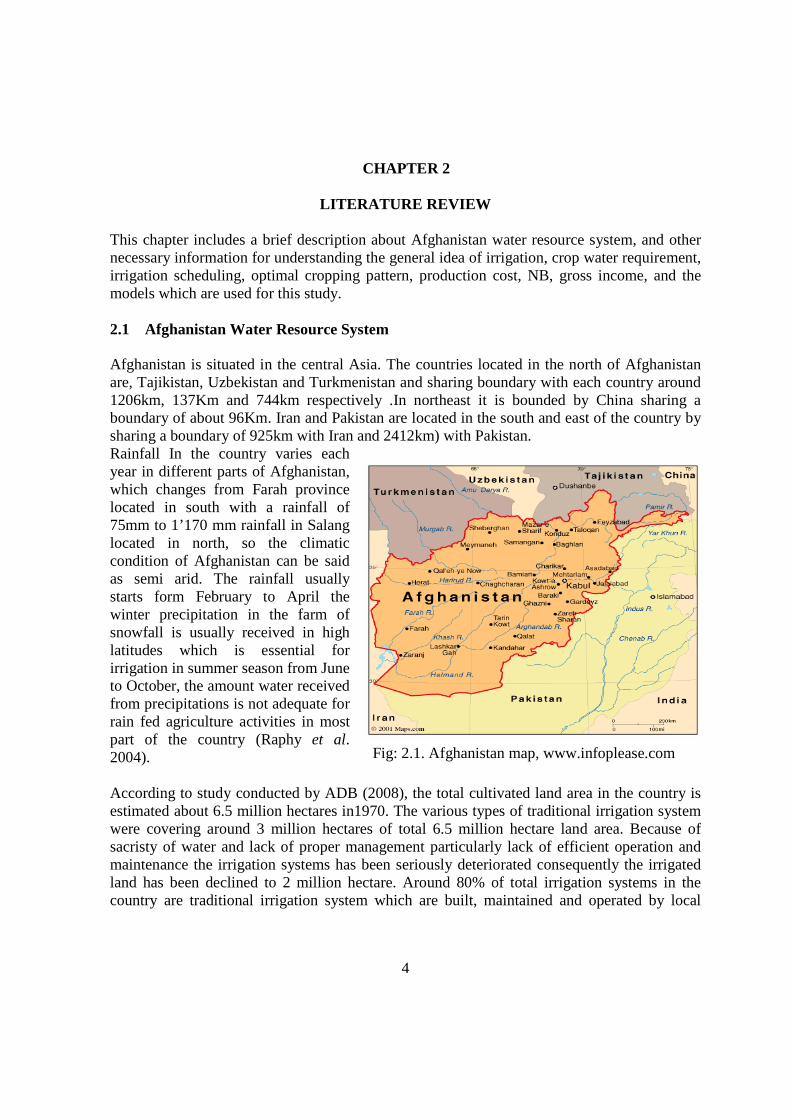
Afghanistan is situated in the central Asia. The countries located in the north of Afghanistan are, Tajikistan, Uzbekistan and Turkmenistan and sharing boundary with each country around 1206km, 137Km and 744km respectively .In northeast it is bounded by China sharing a boundary of about 96Km. Iran and Pakistan are located in the south and east of the country by sharing a boundary of 925km with Iran and 2412km) with Pakistan. Rainfall In the country varies each year in different parts of Afghanistan, which changes from Farah province located in south with a rainfall of 75mm to 1’170 mm rainfall in Salang located in north, so the climatic condition of Afghanistan can be said as semi arid. The rainfall usually starts form February to April the winter precipitation in the farm of snowfall is usually received in high latitudes which is essential for irrigation in summer season from June to October, the amount water received from precipitations is not adequate for rain fed agriculture activities in most part of the country (Raphy et al. 2004). According to study conducted by ADB (2008), the total cultivated land area in the country is estimated about 6.5 million hectares in1970. The various types of traditional irrigation system were covering around 3 million hectares of total 6.5 million hectare land area. Because of sacristy of water and lack of proper management particularly lack of efficient operation and maintenance the irrigation systems has been seriously deteriorated consequently the irrigated land has been declined to 2 million hectare. Around 80% of total irrigation systems in the country are traditional irrigation system which are built, maintained and operated by local

Fig: 2.1. Afghanistan map, www.infoplease.com

5

communities. The irrigation systems in the past was satisfactory up to some extent but the recent turnover have vanished or severely damaged the infrastructures, maintenance and operation and other related services. To prevent more damage it is important to rehabilitate and reconstruct the irrigation systems in the country. The economy of the country is not well developed yet. Around 80% population is settled in rural areas and highly reliable on agriculture and livestock farming. The economy of the country is traditionally based on agriculture sector which is the highest contributor to gross domestic products comparing to the other sectors. Agriculture is the only sector employing around 65 % to total labor force. As Afghanistan is an agrarian country therefore it is entirely reliant on agriculture sector, the water management and irrigation management issues are very important to be considered. (Ministry of Energy & Water) Irrigation productivity for irrigated land area is much higher than rain-fed land, base on a survey in 1978 almost 80% of wheat and 85% total crops produced on irrigation lands. On the other hands at the present water use efficiency is very low merely about 15 to 30 % (Asad, 2002). In Afghanistan water management issues are very important in order to maintain food security and sources of income of huge number of people in rural areas (Rout, 2008). According to Asad (2002), almost 99% irrigation land area irrigation water management is of crucial importance. Because traditional irrigation systems covers around 99% or total 2.3 million hectare irrigated land area of which merely 90% area is coming under the coverage of informal traditional irrigation systems, constructed, operated and maintained by local people (Asad, 2002). Based on FAO report the developed irrigated land was around 1.44 million hectare which can support double cropping of total 2.63 million hectare irrigated land in 1978 (FAO, 1997). Most of irrigation systems in Afghanistan are traditional irrigation system, the water allocation and distribution is based on traditional water right system. The amount of irrigation water tapped in canal irrigation systems from different rivers is around 84.6 %, the water tapped form Karezes was noted around 7 % whereas, water tapped from springs and arhats (shallow tube wells) are 7.9 and 0.5 % respectively (Aini, 2007). Aini (2007) reports based on information from FAO and the Ministry of Energy and Water under the Afghan government that 80 % of Afghanistan water resources highly dependent on amount of precipitation received in a year particularly snow melt in the highland above 2000 m, without contribution of ground water. The amount of water in a year received in highland from snow melt is estimated around 150,000million cubic meter and quantity of water received from rainfall is only 30000million cubic meter in the country. A total of 180,000milion cubic meter received from both rain and snow fall. Merely 15% of total runoff contributes to the ground water discharge (Aini, 2007). According to hydrology department of Ministry of Energy and water based on surface irrigation water, Afghanistan is classified in to five main river basins and into five main non drainage areas.

6

• The Amu Darya Basin in the north of the country flowing from east to west and contributing around 48,120 million cubic meter which is 57% of total surface water in over all country.

• The Hari Rud River Basin flowing toward the west, then north and entering Turkmenistan, and contributing 3,060 million cubic meter which is around 4%of total surface water in Afghanistan.

• The Helmand River Basin flowing toward the south-west and ponds in Hamun-i-Sabiri, contributing 9,300million cum, which is 11% of total surface water in Afghanistan

• The Kabul River Basin flowing toward the east and joining the Indus River in Pakistan, Contributing 21,650million cum, t hat is almost 26% of total surface water over all the country.

• The north flowing river basins that either disappear inside or outside of the country. This river basin contributing around 1,880 million cum, t hat is almost 2% of total surface water over all the country.

2.2 Water Resource Problems in Context of Afghanistan

Water is a main problem both in urban as well as in rural areas because of shortage of water, lack of management and deterioration of water supply schemes. According to FAO news regarding the water issues, water in context of Afghanistan “Water is the lifeblood for the people of Afghanistan, not just for living but also for the economy” more than twenty years of war have damaged much of irrigation systems, infrastructure and other water supply schemes, these are very essential for the agriculture sector economy. The proper management and development of water resources in Afghanistan are essential for sustainability in economic growth. The negative effect on efficiency of irrigation schemes and the capability of communities to maintain and sustain these in traditional methods are the outcomes of around thirty years of war and social conflict. According to FAO (2003) estimation, due to social conflict and severe drought, nearly half of the irrigated land area needs urgent rehabilitation. In order to overcome the problem of water resource in the country and increase agricultural productivity and assure sustainability of agriculture activities practiced on irrigated land, the strategy should be concentrated which focus on enlargement of water capital and assure efficient utilization of water. “For the formulation of strategy for the rehabilitation of irrigation systems, a comprehensive database and information systems should be established. This is absolutely necessary for the accurate and up to date assessment and spatial locations of the rehabilitation work need to be undertaken’’ (Asad, 2002). Basically Afghanistan has limited water resources, which does not make well-organized utilization of amount of available water. Farmers are lack of knowledge of actual irrigation water needs and irrigation scheduling techniques are still mainly based on the amount of

7

maximum water available for a farmer. Therefore present irrigation methods of farmers show a tendency to over irrigate, while the reverse should be accomplished, (Asad, 2002). Currently very little is known regarding water utilization efficiency in context of Afghanistan. However, due to less efficiency water allocation the production from per unit land area is low. Thus further investigation is needed to address the impact of irrigation water allocation, distribution and scheduling on different crops productivity, (Rout, 2008). 2.3 Assessment of Crop Water Requirement

Smajstrla (2002) defined crop water requirement as the total water allocated to fulfill crop’s evapotranspiration demand from irrigation or precipitation hence, it does not decrease the production. Crop evapotranspiration relates to the quantity of water that is lost by evapotranspiration. It is important to verify crop water requirement in order to understanding irrigation demand in better way. Irrigation water requirement is basically understood the variation in the crop water requirements and the effective amount of available precipitation. With Irrigation water requirement we have to consider including the amount of water for leaching of soil and its adjustment for non-uniformity of water application (FAO, 1998). The equations given below are used to estimate the “crop water requirement” (CWR) which is basically equal to the crop evapotranspiration in normal considerations. Having in mind, there are no restraint placed on crop growth like crop density, diseases, water shortage, insects and weeds and salinity pressures. In order to practically compute the actual crop evapotranspiration (ETc), firstly it requires estimating potential or reference Evapotranspiration after that, imposing the proper crop coefficients (Kc).

ETc = Kc x ETo………………………………………………………..……….... (Eq.1) ETc = Crop evapotranspiration in mm/day Kc = crop coefficient, dimensionless ETo = Reference crop evapotranspiration in mm/day

To keep out crop water stress in arid climatic conditions, irrigation and the amount of rainfall must be enough to meet the crop's ET requirement. It means that for any time period throughout the growing season of a crop, the “irrigation water requirement” (IWR) is the quantity of water which is not efficiently provided by rainfall:

IWR= (ET – ER) ……………………………………………………..………….. (Eq.2) IWR= Irrigation Water Requirement needed to satisfy crop water demand, (mm) ET= Evapotranspiration (mm) ER = Effective Rainfall (mm)

8

Fig.2.2. Water balance in root zone, Source: (FAO, 1998)

Irrigation water requirement is the quantity of water that has to be present at crop root region for the crops utilization. To make available (IWR) usually some water wastage happen while moving it from the source of water to the depth of crop root zone because of evaporation and canal percolation. Therefore, more irrigation water must be allocated than the required amount for application in depth of crop root zone. So, this new amount of water called gross irrigation requirement (GIR) which is greater than IWR and to calculate GIR we have to divide IWR by a factor which depends on the irrigation efficiency (Ea).

GIR = IWR / Ea ……………………………………………………….………… (Eq.3) GIR = Gross Irrigation Requirement (mm) Ea = Irrigation Efficiency (always less than one, <1, dimensionless)

The irrigation water requirement may be computed for any time period, it is usually estimated for monthly and seasonal or annual time periods. The concept of a water balance can be defined as an estimation of total amount of water which enter and leave 3D space due to a specific period of time. Burt (1999) mentioned that water balance is not merely limited to irrigation, rainfall, or groundwater. It has to enclose all water which enter and leave the spatial boundaries. Smajstrla (2002) pointed that irrigation water requirement can be estimated by two ways firstly historical observation and secondly numerical models, which numerical model can be based on statistical method or on physical laws that regulate crop consumption and use. Historical observation is a type of estimating crop water requirement, there is a need for long term record of irrigation water application and crop has been repeatedly grown in a location. This information can be useful for estimation of future irrigating demand. It can be desirable to have 20 to 30 years of record and the problem is that little such long term data base exist for computation of accurate values. On the other hand accurate historical data may be obtained from growers or irrigation system managers who may have significant field experience regarding irrigation system and crops. Numerical models can be based on statistical applications or on physical rules that control crop water utilization and consumption. “The Soil Conservation Service” (SCS, 1970) procedure is based on a statistical regression procedure permits crop irrigation need on monthly basis, to be computed according to water-holding features of soil, monthly basis crop ET, amount of monthly rainfall received, and soil information. Application of the model is restricted to surface irrigation system and sprinkler irrigation system, it is because this model

9

can applied for those crops cultivated on the area having deep water table present and furthermore, it can be applied to deep soils which easily drain excess amount of rainfall. Data which is required for soil storage on a typical depth of amount of water applied for a single time of irrigation and it requires assure that applied depth of irrigation water is adequate for water maintaining capacity of soil and for specific crop water requirement (Smajstrla, 2002). To develop the capacity of management of irrigation and utilizing available water resource efficiently and effectively to meet the possible variation of cropping pattern, and making easy management of irrigation practice, it is important to be considered that irrigation management modeling for estimating the various crops water requirement, recent models which are developed through researchers implement on farm water demands with regard to the climate, plant system and Soil briefly explained as below (Sheng, 2001). Smajstrla (1990) developed the “Agricultural Field Scale Irrigation Requirements Simulation” (AFSIRS) model that is a numerical computerized one founded simulation model based on water budget at the crop root region. This model has the capability of calculating amount of irrigation water requirement on annually, seasonal, monthly, two weeks, weekly, and daily basis. Though, a long time historical daily data of Evapotranspiration and amount of precipitation is needed for the model of the site to be simulated. Furthermore, it can estimate extreme as well as mean values of irrigation need. In addition it needs more inputs that clarify crops, soil, components effecting irrigation requirements, as well as irrigation system (Sheng, 2001). Sheng (2001) mentioned that “Crop yield and soil management simulation model” (CRPSM) which is used for estimation of crop production as per soil moisture content availability, different crops and climatic condition during different growing stage has been developed in 1987 by Hill et al. A model of “Unit Command Area” (UCA) that is based partly on the idea of “Crop yield and soil management simulation model” (CRPSM) has been developed by Keller in (1987). This model is created from 2 other sub model: The “on-field sub model” and “water allocation and distribution sub model” to assess and estimate whole (UCA) water requirement and renew water equilibrium in soil on the daily basis (Sheng, 2001). Smith (1991) developed “Decision Support System” CROPWAT for measurement of crop water requirements, irrigation requirement for rice and upland crops and reference evapotranspiration. The most recent CROPWAT version that is to say CROPWAT 4W, which was jointly formulated by the FAO, Southampton University of UK, and National Water Research Center (NWRC) of Egypt, used in a windows interface enclose to a sample water balance model that takes into account the calculation of yield reduction and water stress condition simulation which is grounded on a considerably set up methodologies for finding of crop Evapotranspiration (FAO, 1998).

10

To increase crop potential production by providing water for transferring water, cultivating rice at a proper time and prevent for water stress through an advance system, Chong in (1992) developed the model which has the name of Rice Irrigation Management Model (RIMOD with an improved operation management system (Sheng, 2001). Prajmwong in 1994 originated “Command Area Decision Support Model” (CADSM) the model grounded on 3 other main sub models: firstly weather and field generation, secondly on-field –crop-soil water balance simulation and thirdly water allocation distribution (Sheng, 2001). A genetic algorithm (GA) method was develop under the Irrigation Simulation and Optimization model (ISOM) by Kuo,Sheng-Feng (1995) for maximizing net irrigation project benefits, and to maximize irrigation allocation lands for different crops (Sheng, 2001). 2.4 Irrigation Scheduling

In most developing countries these days irrigation scheduling is just at inception level, although irrigation scheduling is one of the main managerial issues that aim for further efficient water utilization. The raises of competitions among agriculture as well as non-agriculture sectors have increased. Sustainability of irrigation schemes becomes issue of concern, because of increase in agriculture productivity demand and absence of irrigation water resource availability. Therefore water is becoming a limiting factor nearly in all irrigation projects, so these will be guidelines for effective and efficient utilization of water through many water saving techniques. According to Chambers (1983) Irrigation scheduling can be a source of preserving water that supports to make decisions for allocation of quantity and timing of supply of water according to water requirement of different crops. It is the key concern which has the potential to assure the performance to gain sustainability in agriculture farming systems, particularly the stability, productivity, equity and (FAO, 1996). George (2000) pointed down two question has to be answered through irrigation scheduling firstly when to irrigate the crops and secondly how much water should be applied. Irrigation scheduling quantitatively is based on three ideas, namely crop monitoring, soil monitoring and water balance technique. The manner that is based on crop monitoring, leaf water potential or canopy temperature has to be take in to account so the main restriction with this method is that the decision to irrigation is made after the crops has suffered from some amount of moisture stress. Soil moisture monitoring can be useful for irrigation scheduling but, this approach is a bit more time consuming and labor-intensive so it’s not economical. A Soil water balance approach which grounded on irrigation scheduling models, computing soil water over the crops root zone. Many models are developed base on this approach for crops water

11

requirement. And a number of computer based simulation models are develop based on this approach, which is widely approved by researchers and other professionals. Irrigation water management generally has not received sufficient attention from schemes operators but, as struggle for water resources rises up to compound, departments of irrigation in many countries are usually searching for techniques to improve efficiency of water use. Required water management is being usually enclosed in the gorals of lot of rehabilitation projects, with computer-based irrigation scheduling viewed as a promising tool According to Smajstrla et al. (2006) as the constraint of scheduling irrigations are based on plant indicators, thus irrigation is mostly scheduled based on soil water status. The procedure which is used for irrigation scheduling mentioned as below. • Water balance approach grounded on the estimated crop water requirement rate and soil

water storage. • Through a direct measurement of soil water status based on the instrument, and • To combine the above methods in which soil water status instrumentation is used with a

water balance procedure.

The main prior to improve scheduling irrigation efficiency is required to have knowledge of the crop water requirement, root zone depth, and soil water holding capability. Researchers have introduced many techniques for irrigation scheduling for several crops. Mathematical modeling for predicting optimal crop irrigation requirement which is developed has concentrated the attention of many researchers. Cranfield University workshop (2007) proved that irrigation scheduling with the water balance approach is grounded on calculating the soil water content, which is represented with the difference among water that has entered due to rainfall or irrigation and the quantity that has left based on losses (Conveyance, Application, Percolation and Evapotranspiration) from the soil surface and crops. Change in water content of soil is equal to Inputs minus Outputs. If inputs are greater than outputs, in this case the soil is wetter but in inverse case which means, outputs greater than inputs, thus we will have a drier soil. It is common in irrigation to describe the soil water status in terms of a soil water deficit (SWD) instead of soil water content. The SWD can be defined as the difference among the field capacity (FC) water content and present soil water content. A positive soil water deficit shows that soil is drier than field capacity. Therefore, the daily change in soil water deficit equals to outputs minus inputs

If inputs > outputs, it shows a less soil water deficit If outputs > inputs, it shows a greater soil water deficit

12

SWDi - SWDi-1 = ETi-1- Ri-1 - Ii-1………………………………………..…… (Eq.4) To arrange the above equation we will get SWDi = SWDi-1 + ETi-1 - Ri-1 - Ii-1 SWDi = soil water deficit at time i ETi = crop water use at time i Ri = rainfall at time i Ii = irrigation at time i

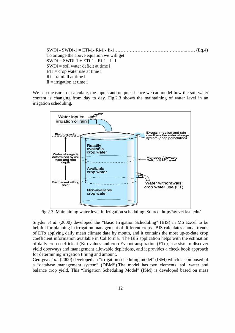
We can measure, or calculate, the inputs and outputs; hence we can model how the soil water content is changing from day to day. Fig.2.3 shows the maintaining of water level in an irrigation scheduling.

Fig.2.3. Maintaining water level in Irrigation scheduling, Source: http://av.vet.ksu.edu/

Snyder et al. (2000) developed the “Basic Irrigation Scheduling” (BIS) in MS Excel to be helpful for planning in irrigation management of different crops. BIS calculates annual trends of ETo applying daily mean climate data by month, and it contains the most up-to-date crop coefficient information available in California. The BIS application helps with the estimation of daily crop coefficient (Kc) values and crop Evapotranspiration (ETc), it assists to discover yield doorways and management allowable depletions, and it provides a check book approach for determining irrigation timing and amount. Georgea et al. (2000) developed an “irrigation scheduling model” (ISM) which is composed of a “database management system” (DBMS).The model has two elements, soil water and balance crop yield. This “Irrigation Scheduling Model” (ISM) is developed based on mass

13

conservation approach and “graphical user interface” (GUI) which has the ability for performing irrigation scheduling under divers management and the option for both single and multiple fields. The data which is needed are climatologically, crops and soil information. In addition the model offers a choice of one or more method for calculating reference Evapotranspiration (ETo). The model was tested against field data and CROPWAT model. Forouda et al. (1992) developed a microcomputer –based simulation model for on farm irrigation. The model simulation was based on daily water balance approach of the crop root zone. The model assumes to address the simulation of crop water in root region, irrigation requirement and soil water. The crop water to be used is estimated from potential Evapotranspiration and the crop coefficient which is suitable for the specific crop and time period. To support farmers in improving the management of on-farm irrigation water; the technical irrigation scheduling activities would be most appropriate tool. The efficiency of irrigation scheduling program should be based on the precise computation of (Crop Evapotranspiration ET) and crop water demand (Aaron, 2005). 2.5 Optimal Cropping Pattern

To investigate optimal cropping pattern and water allocation, whenever water availability is not sufficient to meet the crop water requirement the following factors have to be taken in to account • To emphasis on intensive irrigation to meet crop water requirement and gain maximum net

benefit. • Reduce the cultivated area to make better adjustment based on supply and demand. • To consent the cultivation area with a certain reduction in yield, emphasis for extensive

irrigation to meet partial crop water requirement.

It is absolutely essential to consider more area under cultivation or to increase production per unit area of available land and water resources because, to satisfy the high demand for food to an increasing population. On the other hand it’s crucial to optimize the available land and water resource to get maximum returns, truly it’s difficult to bring additional area under cultivation due to urbanization; moreover the allocation of water for irrigation will probably decrease because of other users like industrials and domestic water usage. Primarily the selecting of crop patterns depend on different crops having different market prices, crop productivities, investment costs, and water demands. Investment costs include the costs of seed, labor, machines, fuel and fertilizer. Crop water demand is very difficult to analyze because it depends on soil conditions, weather conditions and the growth stage of each crop, besides changes in market demands and price structures.

14

The second difficulty is referred with constrains imposed by restricted water resources, and particularly in the dry season, when water level in reservoirs are drawn losing and the amount of rainfall is relatively low. The third difficulty is that the budgets of most farmers are very limited. Linear programming models can be used as an effective tool to optimize cropping pattern in the command areas. The constraints imposed on the objective function of the model should incorporate components that account for farmers’ preference on the area to keep under cultivation of different crops (Singh et al., 2001). 2.6 Production Cost, Gross Income and Net income

All input requirements cost; farmers have access to the inputs they need for production to meet future demand called production cast. Production cost is covering cost of fertilizer, labor force, irrigation, and other operation which is required for the field. Gross income is the income before deductions of production costs; the outcome of yield multiplied by market price is presenting gross income. But the Net income is expressing the entire amount of income that a firm has gain after subtracting production costs and expenses from the total revenue. Net income = ∑ (Gross income – Production C) ……………………………..……….… (Eq.5) Gross income = Market price * yield Production cost = Fertilizer + Labor + Machine + Irrigation + other production cost 2.7 Review of CROPWAT Model

This study finds out the possible solutions for various problems in conditions of improving irrigation water allocation and use in shortage supply context, to be more specific a case study in Jui-Naw area in Herat province of Afghanistan has been taken out. Hereby, to come up with an appropriate and standard calculation for improving irrigation practices through understanding of crop water requirement, planning of cropping options under various irrigation management system, and other assigned relevant objectives and scopes, CROPWAT model, which is a practical tool for helping researcher to analysis results with draw conclusion, is appropriate to apply in context of this study. Further, use of this model is helping to achieve meaningful comparisons results. And another important property of the CROPWAT model is that, it let to have extension of the decisions and conclusions from studies to conditions not tested in the field. Therefore, it can offer practical recommendations to farmers and extension staff on deficit irrigation scheduling under various conditions of water supply, soil, and crop management conditions. CROPWAT is a decision support system, originated by “Land and Water Development Division” of FAO by Smith (1992). In order to estimate “reference evapotranspiration”, “crop

15

water requirement” (CWR) and to support “Irrigation water requirement” (IWR). The algorithm for the estimation CWR and IWR in the model is based on the calculation of the reference evapotranspiration (ETo) which is counting as per Penman-Monteith and other crops parameters. To develop irrigation scheduling under different management system and scheme supply, to evaluate irrigation application efficiency, rain fed production and effect of drought, CROPWAT would be the appropriate tool for developing these all. Climatic and crop data are essential as inputs for CROPWAT. In addition, the CLIMWAT- database is obtained for 144 countries for climate data. The development of irrigation scheduling, rain fed agriculture evaluation and over all irrigation practices are grounded on a daily soil water balance approach using various alternatives in terms of supply and irrigation management system. (Amir, 2001) 2.8 Review of Win-QSB Model

The Quantitative System for Business (QSB) is a capable decision support system which offers range of right tools that is widely used problem–solving algorithms in Operations Research and Management Science (OR/MS). WinQSB is the windows version of QSB software package that runs under the CD-RAM windows. This software was developed by Yih-ong Chang. Professor Hossein Arsham (1994). Almost all the software package uses the simplex algorithm, which is based on Algebraic method. The inputs for solving LP/ILP are given in the following: • The objective function criterion (Max or Min). • The type of each constraint. • The actual coefficients for the problem. • The typical outputs obtained from LP software are: • The optimal values of the objective function. • The optimal values of decision variables. That is, optimal solution. • Reduced cost for objective function value. • Range of optimality for objective function coefficients. Each cost coefficient parameter

can change within this range without affecting the current optimal solution. • The amount of slack or surplus on each constraint depending on whether the constraint is a

resource or a production constraint. • Shadow (or dual) prices for the RHS constraints. We must be careful when applying these

numbers. They are only good for "small" changes in the amounts of resources (i.e., within the RHS sensitivity ranges).

• Ranges of feasibility for right-hand side values. Each RHS coefficient parameter can change within this range without affecting the shadow price for that RHS.

For this study linear programming and Integer linear programming has been used to address the maximization of NB, calories Production and minimization of fertilizer and labors to arise with an appropriate solution for optimizing cropping options.

16

CHEPTER 3

METHODOLOGY

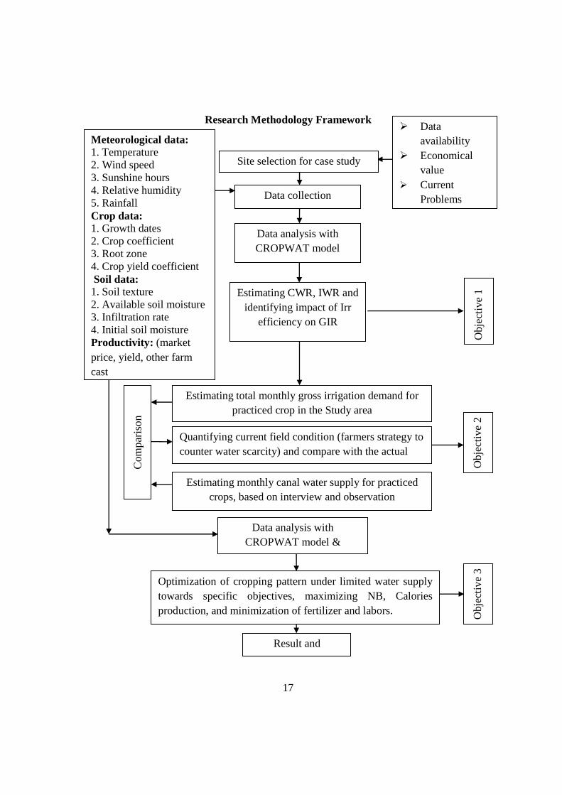
3.1 Research Methodology Framework

In general the concepts of this study comprehend a case Study in Jui-Naw irrigation system in Herat Afghanistan, which is devoted for improving the irrigation water allocation and use for different crops. For this reason the solution ways for relevant problems have been addressed, through the assigned scopes which are the application of CROPWAT model to first estimate crop water requirement (CWR), irrigation water requirement (IWR) and identifying impact of irrigation efficiency on GIR. Secondly, monthly irrigation water demand for practiced crops is estimated in the case study area with the model help thereafter, based on the structured questionnaire and field observation canal water supply is estimated for understanding current field situation on the account of water demand and supply. Thirdly, for investigating possible cropping system on account of optimal and sub-optimal water supply different management scenarios have been tested, as follows; • Reducing area of all crops towards optimal supply of water, and IWR satisfaction, • Eliminating some crops towards optimal supply of water, and IWR satisfaction, • The model also has been used to keep all crops but with sub-optimal supply of water The scenario results have been evaluated from economic and calories production point of view. Quantitative System for Business (Win-QSB), which is an optimization tool that use simplex algorithm, has been used to identify the cropping system option, through the maximization of net economic return (NER), calories production, and minimization of fertilizer and crop labor requirement. Consequently, the suggested methodology conceptual framework for this study is figured out in the next page.

17

Research Methodology Framework

Site selection for case study

� Data availability

� Economical value

� Current Problems Data collection

Data analysis with CROPWAT model

Estimating CWR, IWR and identifying impact of Irr

efficiency on GIR

Data analysis with CROPWAT model &

Obj

ectiv

e 3

Ob

ject

ive

1

Result and discussion

Quantifying current field condition (farmers strategy to counter water scarcity) and compare with the actual crop

Estimating monthly canal water supply for practiced crops, based on interview and observation

Ob

ject

ive

2

Estimating total monthly gross irrigation demand for practiced crop in the Study area

Com

par

iso

n

Optimization of cropping pattern under limited water supply towards specific objectives, maximizing NB, Calories production, and minimization of fertilizer and labors.

Meteorological data: 1. Temperature 2. Wind speed 3. Sunshine hours 4. Relative humidity 5. Rainfall Crop data: 1. Growth dates 2. Crop coefficient 3. Root zone 4. Crop yield coefficient Soil data: 1. Soil texture 2. Available soil moisture 3. Infiltration rate 4. Initial soil moisture Productivity: (market price, yield, other farm cast

18

3.2 Methodology For Over All Objectives

3.2.1 Estimation methodology for CWR and IWR

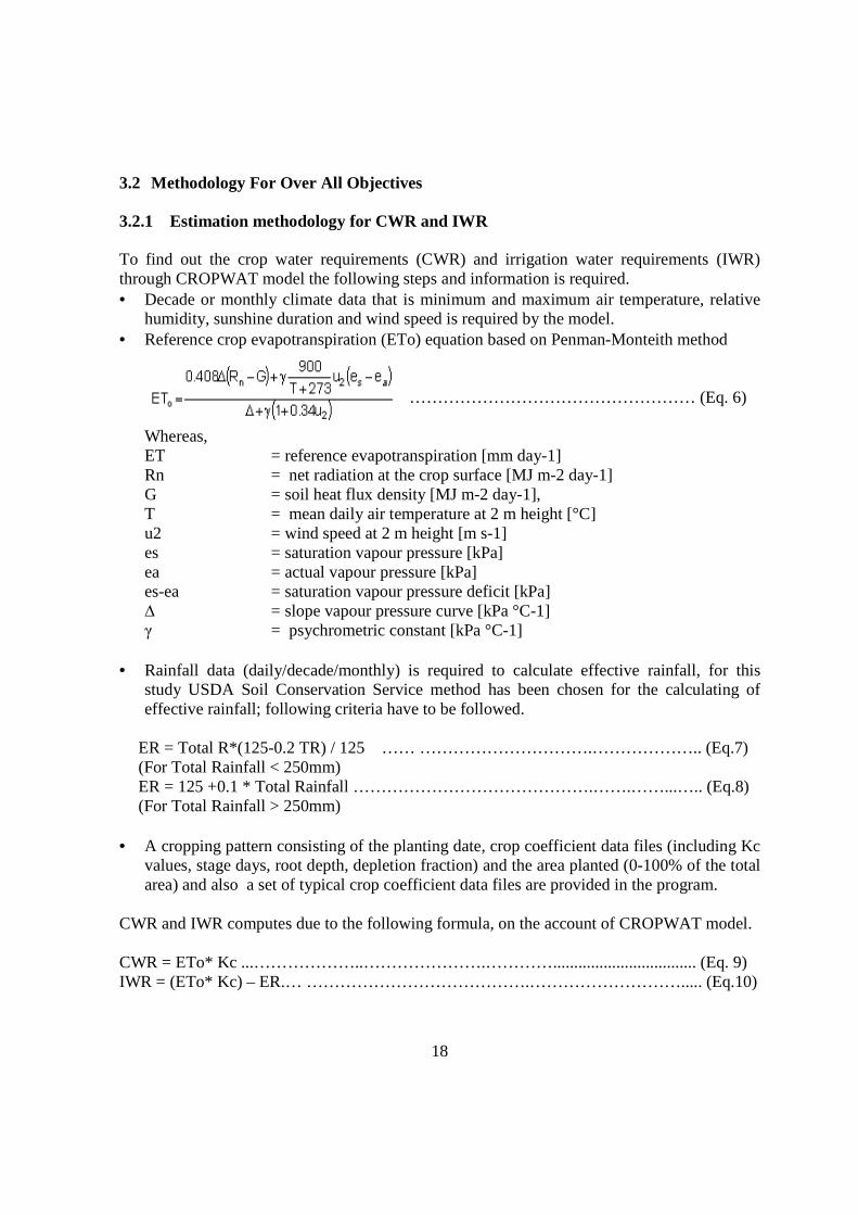
To find out the crop water requirements (CWR) and irrigation water requirements (IWR) through CROPWAT model the following steps and information is required. • Decade or monthly climate data that is minimum and maximum air temperature, relative

humidity, sunshine duration and wind speed is required by the model. • Reference crop evapotranspiration (ETo) equation based on Penman-Monteith method

…………………………………………… (Eq. 6) Whereas, ET = reference evapotranspiration [mm day-1] Rn = net radiation at the crop surface [MJ m-2 day-1] G = soil heat flux density [MJ m-2 day-1], T = mean daily air temperature at 2 m height [°C] u2 = wind speed at 2 m height [m s-1] es = saturation vapour pressure [kPa] ea = actual vapour pressure [kPa] es-ea = saturation vapour pressure deficit [kPa] ∆ = slope vapour pressure curve [kPa °C-1] γ = psychrometric constant [kPa °C-1]

• Rainfall data (daily/decade/monthly) is required to calculate effective rainfall, for this study USDA Soil Conservation Service method has been chosen for the calculating of effective rainfall; following criteria have to be followed.

ER = Total R*(125-0.2 TR) / 125 …… ………………………….……………….. (Eq.7) (For Total Rainfall < 250mm) ER = 125 +0.1 * Total Rainfall …………………………………….…….……...….. (Eq.8) (For Total Rainfall > 250mm)

• A cropping pattern consisting of the planting date, crop coefficient data files (including Kc values, stage days, root depth, depletion fraction) and the area planted (0-100% of the total area) and also a set of typical crop coefficient data files are provided in the program.

CWR and IWR computes due to the following formula, on the account of CROPWAT model. CWR = ETo* Kc ...………………..………………….………….................................. (Eq. 9) IWR = (ETo* Kc) – ER.… ………………………………….………………………..... (Eq.10)

19

3.2.2 Estimation methodology for irrigation scheduling

To estimate Irrigation Scheduling these options should be taken in to account • Defined times, date, and depth by users • Application timing • Irrigate when a specified % of Readily Soil Moisture Depletion occurs. • Irrigate when a specified % of Total Soil Moisture Depletion occurs. • Irrigate when a specified % of Soil Moisture Depletion occurs. • Irrigate at Fixed Intervals (day). • Irrigate at Variable Intervals (User- Defined) (days) • Application Depths • Refill to a specified % of Readily Available Soil Moisture. • Fixed Depths (mm). • Variable Depths (user- Defined) (mm).

Model requires information on, Soil type, total available soil moisture, maximum rooting depth and initial soil moisture depletion (% of total available moisture). The best scenario will be select based on existing cropping pattern and site adaptability. Hence, after fixing scheduling have to find out the actual crop water requirement and irrigation water requirement. 3.2.3 Estimation methodology for comparison of current and actual field condition

For understating the current and actual field situation it’s required to know how much water is given for difference crops in each month for the practiced crops in the study area, with the existing irrigations efficiency, secondly it’s necessary to explore monthly canal available water for the crops in the study area. CROPWAT is taken in account for simulating the net irrigation requirement of each crop in the study area, and canal flow is estimated based on the rectangular weir formula. The result of this scenario helps to quantify that which crops are suffering from water shortage, which is an important factor for yield reduction, and which crops are not facing water scarcity and what are farmers measure in case of water shortage. 3.2.4 Estimation methodology for optimization of cropping pattern

The result from the previous objectives helps to understand the real field condition, and it would be better guild for appropriate decision for optimizing cropping patterns. Different scenarios are tested for understanding the optimal situation, reducing area of all crops and optimal supply of water, eliminating some crops and optimal supply of water, and last the model also has been used to schedule the sub-optimal supply for all practiced crops. The WinQSB, which is an optimization technique tool, has been taken in account to help for identifying cropping system options, with respect to the maximization of net economic return (NER), calories production, and minimization of fertilizer and labor under limited water supply.

20

The scenario results have been evaluated from economic and calories production point of view. The information which is needed to address the economic assessment are, yield, market price, and production cost. The component which are involve in production cost are, fertilizer, labor, irrigation cost and finally field operation cost if exist. Understanding calories contents of practiced crops is required for maximizing calories production due to available water and land. 3.2.5 CROPWAT model output

Once all the data is entered, CROPWAT 4 Windows automatically calculates the results as tables or plotted in graphs. The time step of the results can be any convenient time step: daily, weekly, decade or monthly. The output parameters for each crop in the cropping pattern are

• Reference crop Evapotranspiration – ETo (mm/period) • Crop Kc - average values of crop coefficient for each time step • Effective rain (mm/period) - the amount of water that enters the soil • Crop water requirements – CWR or Etm (mm/period) • Irrigation requirements –IWR (mm/period) • Total available moisture –TAM (mm) • Readily available moisture – RAM (mm) • Actual crop Evapotranspiration – ETc (mm) • Ratio of actual crop Evapotranspiration to the maximum crop

evapotranspiration ETc/ETm (%). • Daily soil moisture deficit (mm) • Irrigation interval (days) & irrigation depth applied (mm) • Lost irrigation (mm)– irrigation water that is not stored in the soil (i.e. either

surface Runoff or percolation) • Estimated yields reduction due to crop stress when (Etc/Etm) falls below

hundred percent. Following Eq.8 represents crops yield reduction in CROPWAT mode in each stage of crops life.

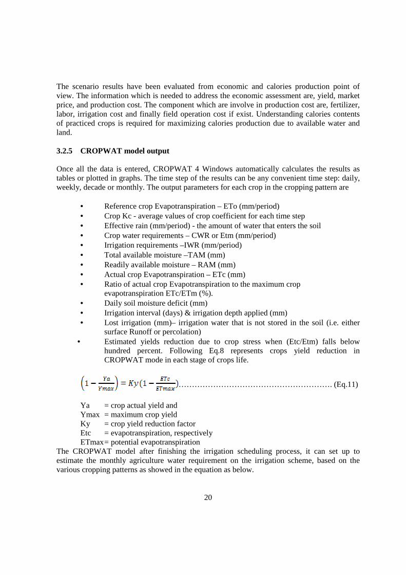
…………………………………………………. (Eq.11)

Ya = crop actual yield and Ymax = maximum crop yield Ky = crop yield reduction factor Etc = evapotranspiration, respectively ETmax = potential evapotranspiration

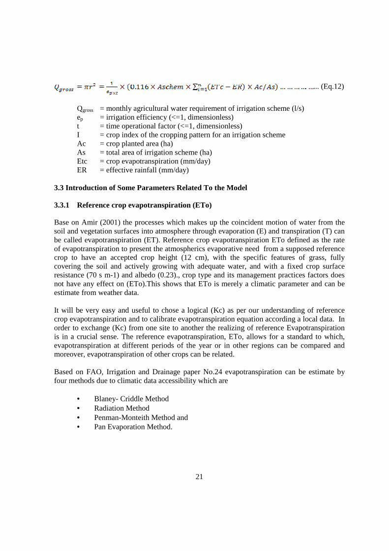
The CROPWAT model after finishing the irrigation scheduling process, it can set up to estimate the monthly agriculture water requirement on the irrigation scheme, based on the various cropping patterns as showed in the equation as below.

21

... (Eq.12)

Qgross = monthly agricultural water requirement of irrigation scheme (l/s) ep = irrigation efficiency (<=1, dimensionless) t = time operational factor (<=1, dimensionless) I = crop index of the cropping pattern for an irrigation scheme Ac = crop planted area (ha) As = total area of irrigation scheme (ha) Etc = crop evapotranspiration (mm/day) ER = effective rainfall (mm/day)

3.3 Introduction of Some Parameters Related To the Model

3.3.1 Reference crop evapotranspiration (ETo)

Base on Amir (2001) the processes which makes up the coincident motion of water from the soil and vegetation surfaces into atmosphere through evaporation (E) and transpiration (T) can be called evapotranspiration (ET). Reference crop evapotranspiration ETo defined as the rate of evapotranspiration to present the atmospherics evaporative need from a supposed reference crop to have an accepted crop height (12 cm), with the specific features of grass, fully covering the soil and actively growing with adequate water, and with a fixed crop surface resistance (70 s m-1) and albedo (0.23)., crop type and its management practices factors does not have any effect on (ETo).This shows that ETo is merely a climatic parameter and can be estimate from weather data. It will be very easy and useful to chose a logical (Kc) as per our understanding of reference crop evapotranspiration and to calibrate evapotranspiration equation according a local data. In order to exchange (Kc) from one site to another the realizing of reference Evapotranspiration is in a crucial sense. The reference evapotranspiration, ETo, allows for a standard to which, evapotranspiration at different periods of the year or in other regions can be compared and moreover, evapotranspiration of other crops can be related. Based on FAO, Irrigation and Drainage paper No.24 evapotranspiration can be estimate by four methods due to climatic data accessibility which are

• Blaney- Criddle Method • Radiation Method • Penman-Monteith Method and • Pan Evaporation Method.

22

Suat (2003) International Commission for Irrigation and Drainage (ICID) and the Food and Agriculture Organization of the United Nations (UNFAO) expert consultation highly recommend the Penman-Monteith method for estimation of evapotranspiration than other methods, because this method is used as the standard method and encompasses both physical and aerodynamic parameters. In addition with this method a process has developed to calculate the missing climatic data. Moreover Penman glide path in both arid and humid region has been showed very accurate and logical in both ASCE and European research studies. 3.3.2 Crop coefficient (Kc)

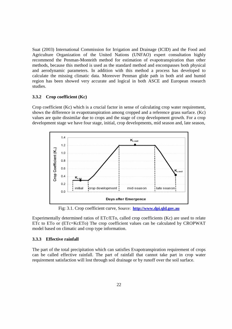
Crop coefficient (Kc) which is a crucial factor in sense of calculating crop water requirement, shows the difference in evapotranspiration among cropped and a reference grass surface. (Kc) values are quite dissimilar due to crops and the stage of crop development growth. For a crop development stage we have four stage, initial, crop developments, mid season and, late season,

Fig: 3.1. Crop coefficient curve, Source: http://www.dpi.qld.gov.au

Experimentally determined ratios of ETc/ETo, called crop coefficients (Kc) are used to relate ETc to ETo or (ETc=KcETo) The crop coefficient values can be calculated by CROPWAT model based on climatic and crop type information. 3.3.3 Effective rainfall The part of the total precipitation which can satisfies Evapotranspiration requirement of crops can be called effective rainfall. The part of rainfall that cannot take part in crop water requirement satisfaction will lost through soil drainage or by runoff over the soil surface.

23

Four methods for estimating effective rainfall derived from experiment and observation (Smith 1991) firstly fixed percentage of rainfall, secondly dependable rainfall thirdly empirical formula, and lastly USDA Soil Conservation Service Method. � Fixed percentage of rainfall: In this method a typical range between 0.7 up to 0.9 will

consider by model user as a specific coefficient, ER = a * R……..…………………………………………………………....…... (Eq.13) a = specific coefficient ER = Effective rainfall R = Total rainfall

� Dependable rainfall: This method which is developed by FAO can be used more for designing purpose to estimate dependable rainfall. ER= 0.6TR – 10…………….………………………………………………...… (Eq.14) This equation is valid where (TR < 70mm) ER= 0.8TR – 24………………………………………………………………… (Eq.15) Equation 12, is valid when (TR>70 mm) ER = Effective Rainfall TR = Total Rainfall

� Empirical formula: This method grounded on analyzing the formula which is dependent on local climatic data to determine the effective rainfall. ER = a (Total Rain) + b……..……………………………...…...………………. (Eq.16) For TR < z mm ER = c (Total Rain) + d……..…………………………………….......………… (Eq.17) For TR > z mm Where a, b, c, d and z are empirically derived correction coefficients

� USDA Soil Conservation Service method: In this case we have the bellow criteria ER = Total Rain = ……..……………………...…………………...…............ (Eq.18) For Total Rainfall < 250mm ER= 125 +0.1 * Total Rainfall……..………………………………………..... (Eq.19) For Total Rainfall > 250mm)

3.3.4 Total available moisture and readily available moisture

The field capacity minus permanent wilting point multiplying to crop rooting depth can be called (TAM).On the other hands, to avoid crops from water stress soil moisture should be kept above the Readily available moisture which can be define as the result of multiplication of TAM to depletion friction factor that is P, (FAO, 1998). RAM = TAM* P ……. ………………………………………………………………. (Eq.20)

24

CHAPTER 4

DATA ANALYSIS AND RESULTS

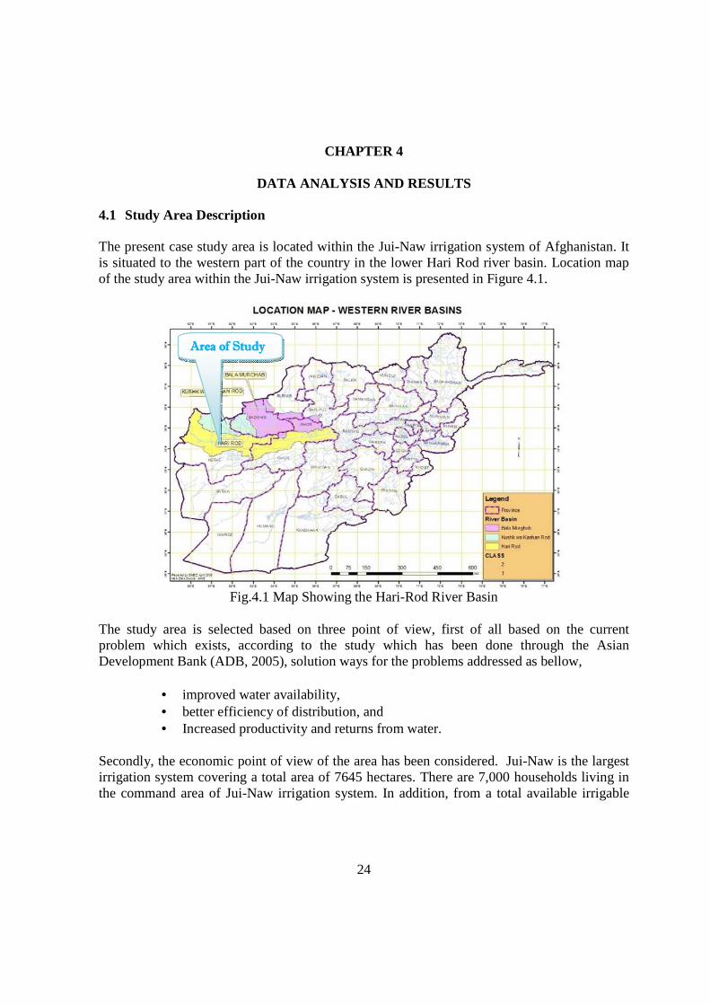
4.1 Study Area Description

The present case study area is located within the Jui-Naw irrigation system of Afghanistan. It is situated to the western part of the country in the lower Hari Rod river basin. Location map of the study area within the Jui-Naw irrigation system is presented in Figure 4.1.

Fig.4.1 Map Showing the Hari-Rod River Basin

The study area is selected based on three point of view, first of all based on the current problem which exists, according to the study which has been done through the Asian Development Bank (ADB, 2005), solution ways for the problems addressed as bellow,

• improved water availability, • better efficiency of distribution, and • Increased productivity and returns from water.

Secondly, the economic point of view of the area has been considered. Jui-Naw is the largest irrigation system covering a total area of 7645 hectares. There are 7,000 households living in the command area of Jui-Naw irrigation system. In addition, from a total available irrigable

Area of StudyArea of StudyArea of StudyArea of Study

25

area of 5,133 hectares in system, only 50% of the cultivable area can be irrigated (ADB, 2005). Table 4.1 presents the summary of command and irrigable areas for the three sections

Table.4.1. Command and Irrigable Area in Jui-Naw Irrigation System (ADB, 2008)

Section Area (ha)

Command Irrigable

Upper 2637 1928 Middle 2601 1901 Lower 2407 1304 Total 7645 5133

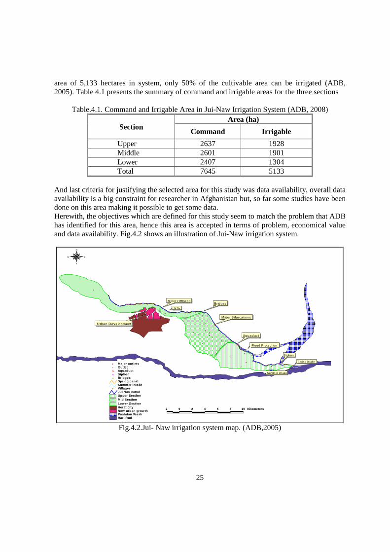
And last criteria for justifying the selected area for this study was data availability, overall data availability is a big constraint for researcher in Afghanistan but, so far some studies have been done on this area making it possible to get some data. Herewith, the objectives which are defined for this study seem to match the problem that ADB has identified for this area, hence this area is accepted in terms of problem, economical value and data availability. Fig.4.2 shows an illustration of Jui-Naw irrigation system.

#Y

#Y

#Y

#Y

#Y

#Y

#Y

#Y

#Y

#Y

#Y#Y

#Y

#Y

#Y

#Y

#Y

#Y

#Y

#Y

%a

%a

%a%a%a%a%a%a%a%a%a%a%a%a

%a%a%a

%a%a%a

%a%a

%a%a

%a%a%a%a%a%a%a %a%a

%a%a%a%a%a%a%a%a%a%a%a%a%a%a%a%a%a%a%a%a %a%a%a%a

%a

%%

%

######

#

#

##

##

#

#

##

##

#

##

#

######### #####

####

##################

#

#

#³

#³

#³

#³

#³

#³

#³

#³

#³#³#³#³#³#³#³#³

#³

Aquaduct

Siphon

Major B ifurcations

Minor Offtakes

Urban Development

Bridges

Flood Protection

Summ er intake

Spring intake

UX Os

Hari RudPashdan WashNew urban growthHerat cityLower SectionMid SectionUpper SectionJui Nau canal

#Y VillagesSummer intakeSpring canal

%a Bridges% Siphon% Aquaduct# Outlet#³ Major outlets

2 0 2 4 6 8 10 Kilometers

N

EW

S

Fig.4.2.Jui- Naw irrigation system map. (ADB,2005)

26

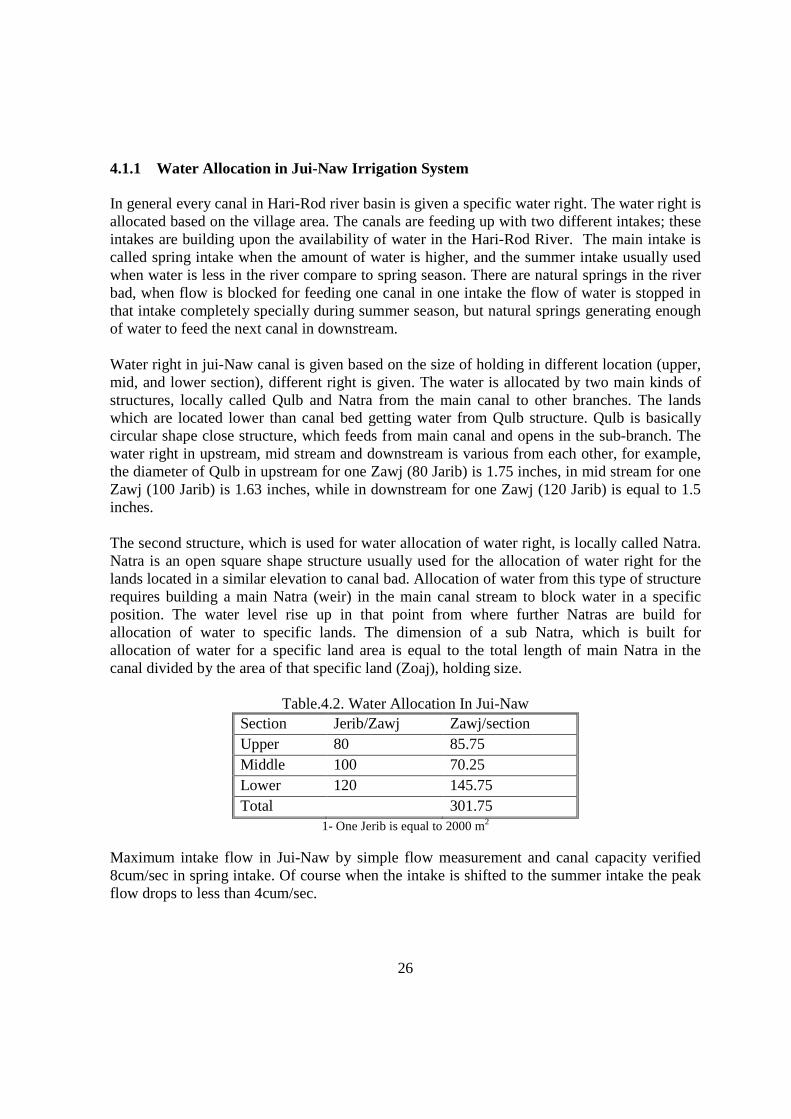
4.1.1 Water Allocation in Jui-Naw Irrigation System

In general every canal in Hari-Rod river basin is given a specific water right. The water right is allocated based on the village area. The canals are feeding up with two different intakes; these intakes are building upon the availability of water in the Hari-Rod River. The main intake is called spring intake when the amount of water is higher, and the summer intake usually used when water is less in the river compare to spring season. There are natural springs in the river bad, when flow is blocked for feeding one canal in one intake the flow of water is stopped in that intake completely specially during summer season, but natural springs generating enough of water to feed the next canal in downstream. Water right in jui-Naw canal is given based on the size of holding in different location (upper, mid, and lower section), different right is given. The water is allocated by two main kinds of structures, locally called Qulb and Natra from the main canal to other branches. The lands which are located lower than canal bed getting water from Qulb structure. Qulb is basically circular shape close structure, which feeds from main canal and opens in the sub-branch. The water right in upstream, mid stream and downstream is various from each other, for example, the diameter of Qulb in upstream for one Zawj (80 Jarib) is 1.75 inches, in mid stream for one Zawj (100 Jarib) is 1.63 inches, while in downstream for one Zawj (120 Jarib) is equal to 1.5 inches. The second structure, which is used for water allocation of water right, is locally called Natra. Natra is an open square shape structure usually used for the allocation of water right for the lands located in a similar elevation to canal bad. Allocation of water from this type of structure requires building a main Natra (weir) in the main canal stream to block water in a specific position. The water level rise up in that point from where further Natras are build for allocation of water to specific lands. The dimension of a sub Natra, which is built for allocation of water for a specific land area is equal to the total length of main Natra in the canal divided by the area of that specific land (Zoaj), holding size.

Table.4.2. Water Allocation In Jui-Naw Section Jerib/Zawj Zawj/section Upper 80 85.75 Middle 100 70.25 Lower 120 145.75 Total 301.75

1- One Jerib is equal to 2000 m2 Maximum intake flow in Jui-Naw by simple flow measurement and canal capacity verified 8cum/sec in spring intake. Of course when the intake is shifted to the summer intake the peak flow drops to less than 4cum/sec.

27

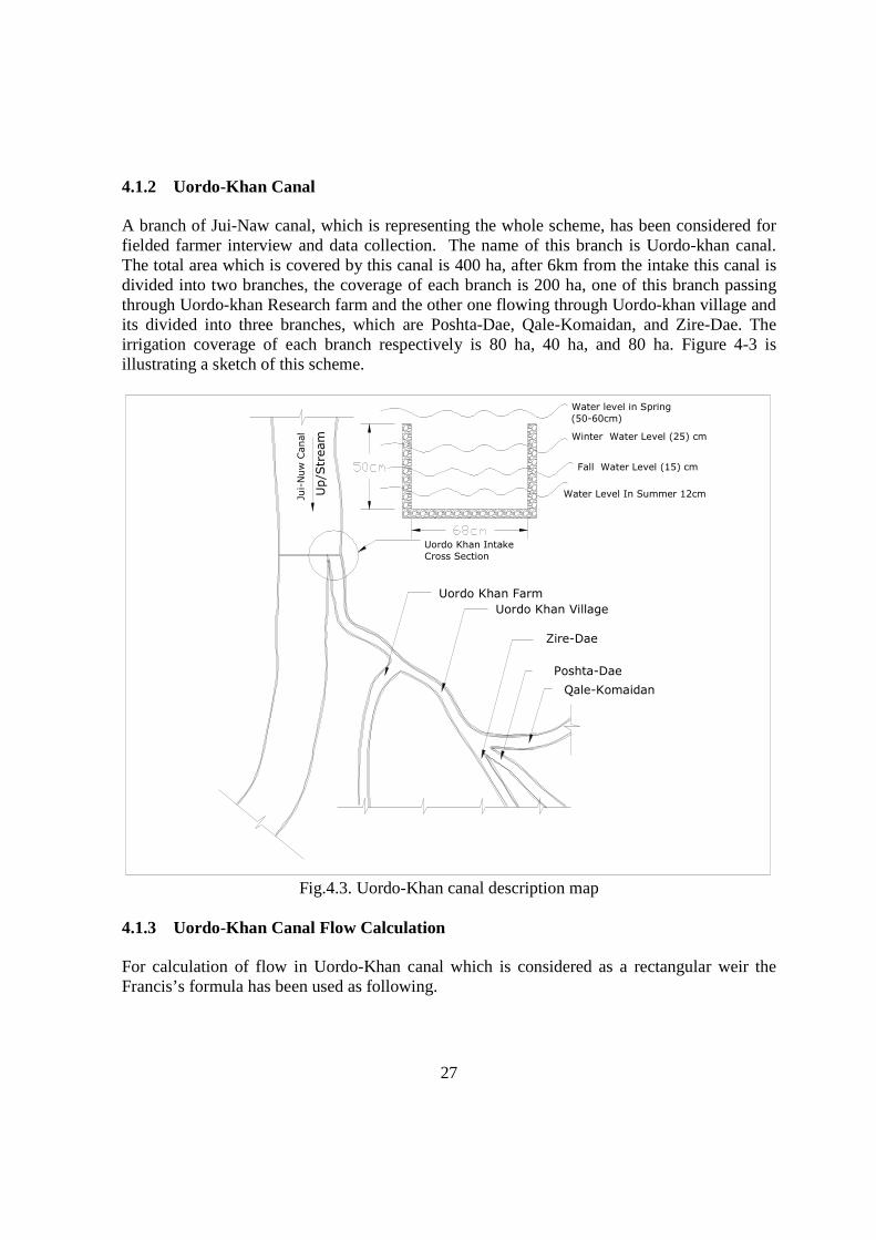
4.1.2 Uordo-Khan Canal

A branch of Jui-Naw canal, which is representing the whole scheme, has been considered for fielded farmer interview and data collection. The name of this branch is Uordo-khan canal. The total area which is covered by this canal is 400 ha, after 6km from the intake this canal is divided into two branches, the coverage of each branch is 200 ha, one of this branch passing through Uordo-khan Research farm and the other one flowing through Uordo-khan village and its divided into three branches, which are Poshta-Dae, Qale-Komaidan, and Zire-Dae. The irrigation coverage of each branch respectively is 80 ha, 40 ha, and 80 ha. Figure 4-3 is illustrating a sketch of this scheme.

Zire-Dae

Jui-Nuw C

anal

Up/S

tream

Uordo Khan Farm

Uordo Khan Village

Poshta-Dae

Qale-Komaidan

Uordo Khan Intake

Cross Section

Water level in Spring

(50-60cm)

Winter Water Level (25) cm

Water Level In Summer 12cm

Fall Water Level (15) cm

Fig.4.3. Uordo-Khan canal description map

4.1.3 Uordo-Khan Canal Flow Calculation

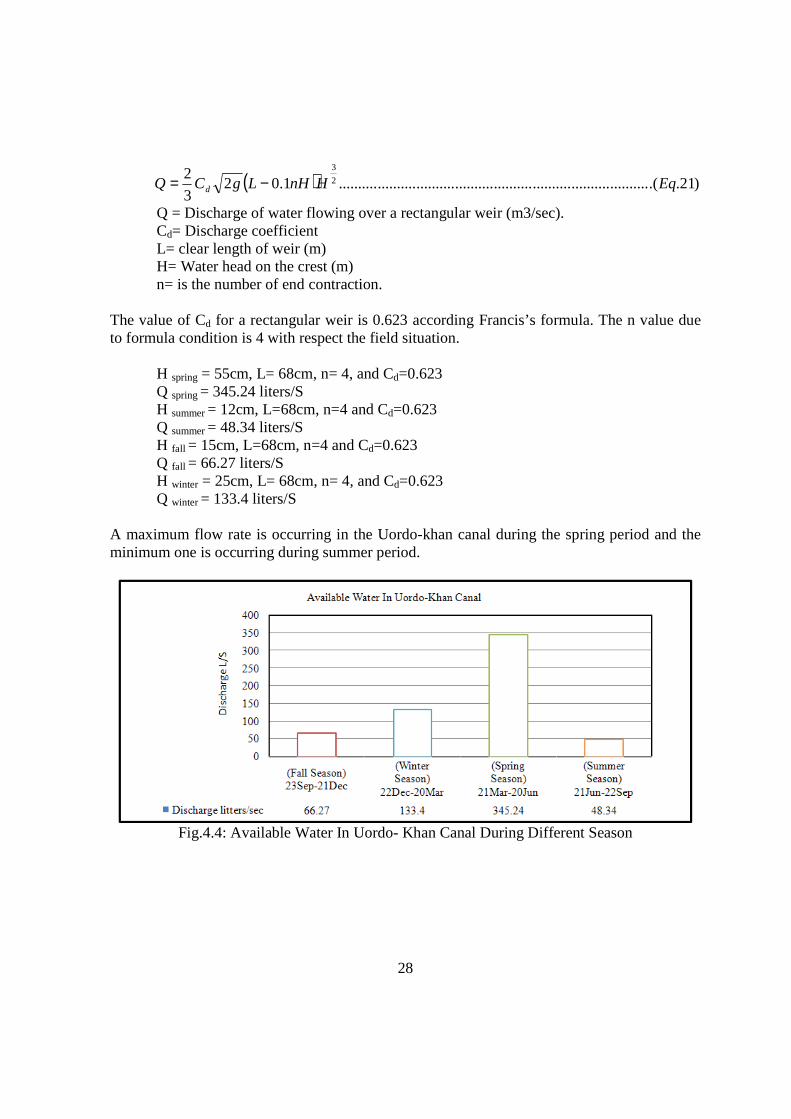
For calculation of flow in Uordo-Khan canal which is considered as a rectangular weir the Francis’s formula has been used as following.

28

Q = Discharge of water flowing over a rectangular weir (m3/sec). Cd= Discharge coefficient L= clear length of weir (m) H= Water head on the crest (m) n= is the number of end contraction.

The value of Cd for a rectangular weir is 0.623 according Francis’s formula. The n value due to formula condition is 4 with respect the field situation.

H spring = 55cm, L= 68cm, n= 4, and Cd=0.623 Q spring = 345.24 liters/S H summer = 12cm, L=68cm, n=4 and Cd=0.623 Q summer = 48.34 liters/S H fall = 15cm, L=68cm, n=4 and Cd=0.623 Q fall = 66.27 liters/S H winter = 25cm, L= 68cm, n= 4, and Cd=0.623 Q winter = 133.4 liters/S

A maximum flow rate is occurring in the Uordo-khan canal during the spring period and the minimum one is occurring during summer period.

Fig.4.4: Available Water In Uordo- Khan Canal During Different Season

( ) )21..(................................................................................1.023

2 2

3

EqHnHLgCQ d −=

29

4.2 Fieldwork

Fieldwork has been covered almost all the necessary hydro-Metrological data, which are necessary as input for CROPWAT model, as well as farmer interview throughout structured questionnaire and formal interviews with various groups about agriculture water use, water allocation, irrigation methods and crop calendar. Reconnaissance survey has been carried out for identifying the site and gaining information about the current situation in the field. All over, 50 farmers was conducted to a formal interview for collecting primary farm information, cultivated area, water allocation system, crop type and rotation, irrigation scheduling, irrigation practice and furthermore, farmers were called for sharing their knowledge on alternative cropping pattern and water supply sources. The secondary data was collected from various governmental and non-governmental both national and international organization involved in related studies. Of course, some information like soil, crop coefficient, crop rooting depth and crop yield response factor has been gathered through review of various reliable publications.

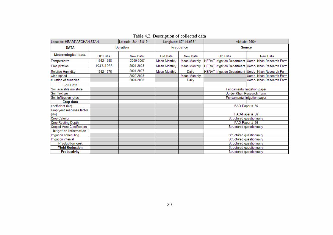
30

Table 4.3. Description of collected data

31

4.3 Metrological Data Analysis

The required climatic data from 1942 to 1988 has been collected from Irrigation department. The climatic data from 1988 to 2000 is not available, because of interior country conflicts. The recent climatic information from 2001 to 2008 has been collected from Urdo-khan Research Farm. 4.3.1 Rainfall Data

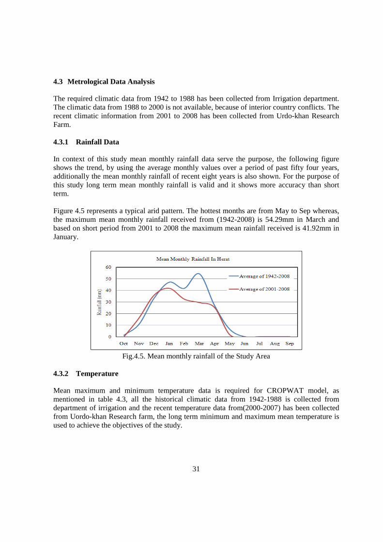
In context of this study mean monthly rainfall data serve the purpose, the following figure shows the trend, by using the average monthly values over a period of past fifty four years, additionally the mean monthly rainfall of recent eight years is also shown. For the purpose of this study long term mean monthly rainfall is valid and it shows more accuracy than short term. Figure 4.5 represents a typical arid pattern. The hottest months are from May to Sep whereas, the maximum mean monthly rainfall received from (1942-2008) is 54.29mm in March and based on short period from 2001 to 2008 the maximum mean rainfall received is 41.92mm in January.

Fig.4.5. Mean monthly rainfall of the Study Area

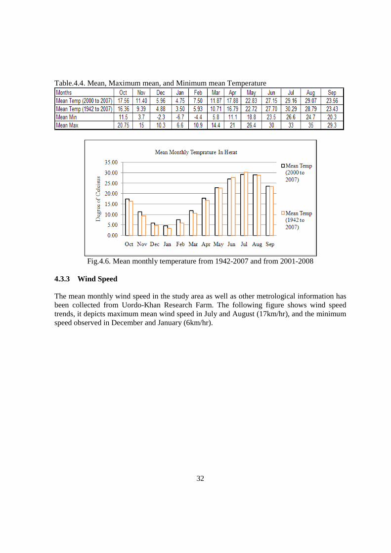
4.3.2 Temperature

Mean maximum and minimum temperature data is required for CROPWAT model, as mentioned in table 4.3, all the historical climatic data from 1942-1988 is collected from department of irrigation and the recent temperature data from(2000-2007) has been collected from Uordo-khan Research farm, the long term minimum and maximum mean temperature is used to achieve the objectives of the study.

32

Table.4.4. Mean, Maximum mean, and Minimum mean Temperature

Fig.4.6. Mean monthly temperature from 1942-2007 and from 2001-2008

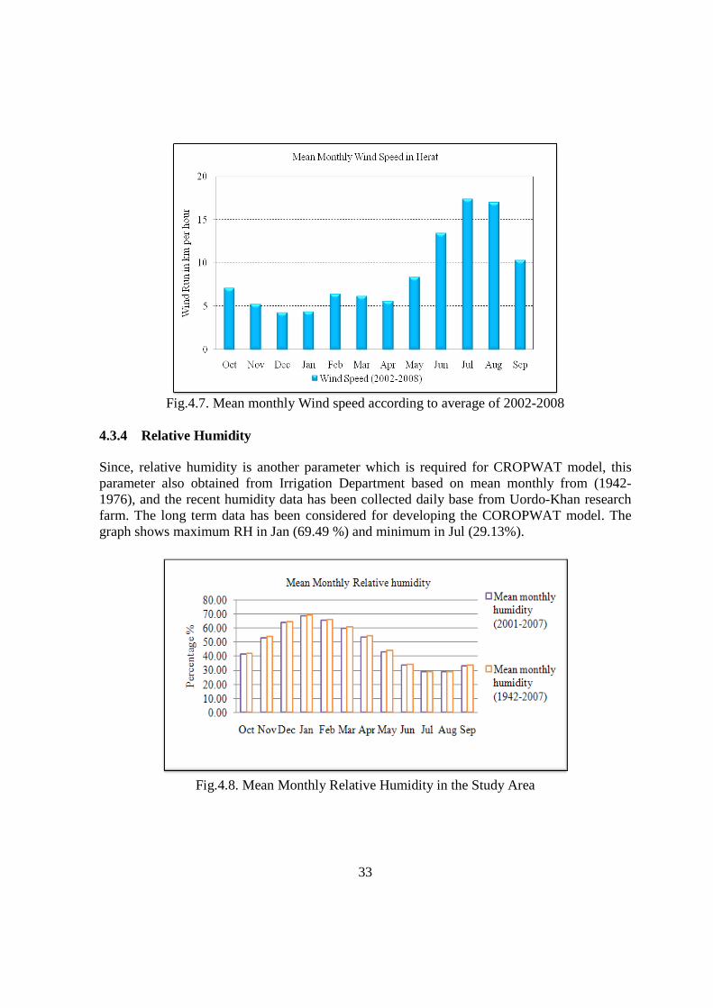
4.3.3 Wind Speed

The mean monthly wind speed in the study area as well as other metrological information has been collected from Uordo-Khan Research Farm. The following figure shows wind speed trends, it depicts maximum mean wind speed in July and August (17km/hr), and the minimum speed observed in December and January (6km/hr).

33

Fig.4.7. Mean monthly Wind speed according to average of 2002-2008

4.3.4 Relative Humidity

Since, relative humidity is another parameter which is required for CROPWAT model, this parameter also obtained from Irrigation Department based on mean monthly from (1942-1976), and the recent humidity data has been collected daily base from Uordo-Khan research farm. The long term data has been considered for developing the COROPWAT model. The graph shows maximum RH in Jan (69.49 %) and minimum in Jul (29.13%).

Fig.4.8. Mean Monthly Relative Humidity in the Study Area

34

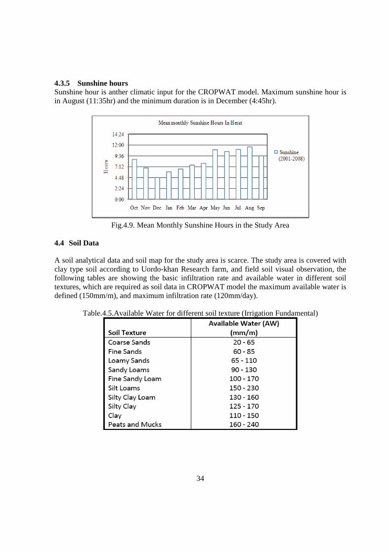
4.3.5 Sunshine hours Sunshine hour is anther climatic input for the CROPWAT model. Maximum sunshine hour is in August (11:35hr) and the minimum duration is in December (4:45hr).

Fig.4.9. Mean Monthly Sunshine Hours in the Study Area

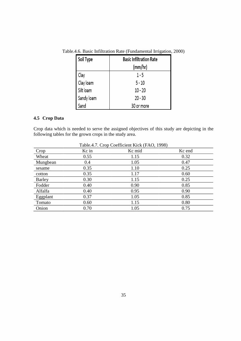
4.4 Soil Data

A soil analytical data and soil map for the study area is scarce. The study area is covered with clay type soil according to Uordo-khan Research farm, and field soil visual observation, the following tables are showing the basic infiltration rate and available water in different soil textures, which are required as soil data in CROPWAT model the maximum available water is defined (150mm/m), and maximum infiltration rate (120mm/day).

Table.4.5.Available Water for different soil texture (Irrigation Fundamental)

35

Table.4.6. Basic Infiltration Rate (Fundamental Irrigation, 2000)

4.5 Crop Data

Crop data which is needed to serve the assigned objectives of this study are depicting in the following tables for the grown crops in the study area.

Table.4.7. Crop Coefficient Kick (FAO, 1998) Crop Kc in Kc mid Kc end Wheat 0.55 1.15 0.32 Mungbean 0.4 1.05 0.47 sesame 0.35 1.10 0.25 cotton 0.35 1.17 0.60 Barley 0.30 1.15 0.25 Fodder 0.40 0.90 0.85 Alfalfa 0.40 0.95 0.90 Eggplant 0.37 1.05 0.85 Tomato 0.60 1.15 0.80 Onion 0.70 1.05 0.75

36

Table.4.8. Rooting Depth, Yield Response factor (Ky) and Depletion Fraction (P) (FAO, 1998; Fundamental Irrigation) Crop Rooting Depth (m) Yield Response factor (Ky) Depletion Fraction (P) Wheat 1.5-1.8 0.2 0.6 0.5 0.5 0.55 Mungbean 0.6-1 0.2 1.1 0.75 0.2 0.45 sesame 1-1.5 0.4 0.4 0.4 0.4 0.6 cotton 1-1.7 0,2 0.5 0.4 0.25 0.65 Barley 1-1.5 0.2 0.6 0.5 0.5 0.55 Fodder 0.6-0.9 0.7 0.7 0.7 0.7 0.5 Alfalfa 0.65-1 0.7 0.7 0.7 0.7 0.55 Eggplant 0.7-1.2 0.45 0.45 0.8 0.3 0.45 Tomato 0.7-1.5 0.4 1,1 0.8 0.4 0.4 Onion 0.3-0.5 0.45 0.45 0.8 0.3 0.3

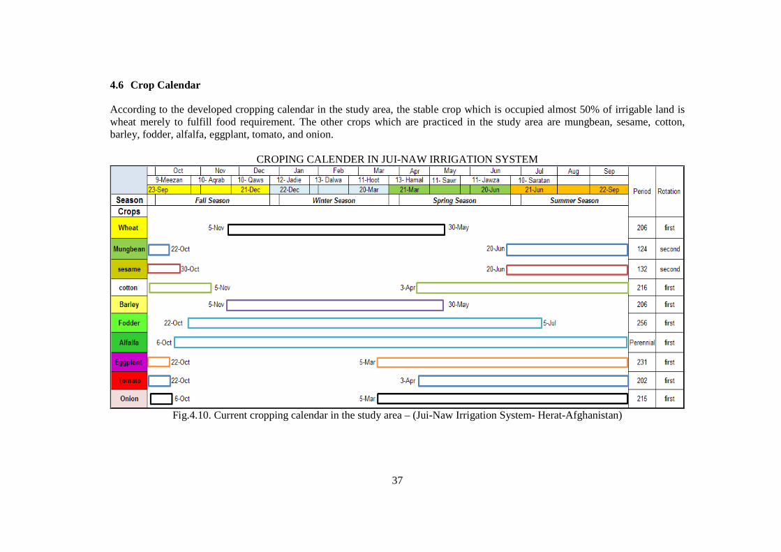
37

4.6 Crop Calendar

According to the developed cropping calendar in the study area, the stable crop which is occupied almost 50% of irrigable land is wheat merely to fulfill food requirement. The other crops which are practiced in the study area are mungbean, sesame, cotton, barley, fodder, alfalfa, eggplant, tomato, and onion.

CROPING CALENDER IN JUI-NAW IRRIGATION SYSTEM

Fig.4.10. Current cropping calendar in the study area – (Jui-Naw Irrigation System- Herat-Afghanistan)

38

Following figure.4.11 shows percentages of different crops currently cultivated in the study area. The graph reveals that farmers intend to allocate more lands for crops they can cultivated during the winter season, because they think their lands do not need more irrigation water, therefore more land is allocated for crops cultivate in the fall season and harvested in spring season. Due to water shortage in the study area farmers prefer to reduce their cropped land when they feel water is not sufficient to meet the demand therefore, they are not even able to cultivate the available land in the study area. Cropping intensity in the study area is calculated 75 % that means 25% of the available lands are not covering any plants.

Fig.4.11: Cropping parcentage in the study area

Wheat and barley are covering respectively 50 and 12 percent of the study area, because wheat is the staple food in the area and all farmers prefer to cultivate wheat to supply their households demand. Furthermore, the farmers cultivate these crops with the hope that they will receive precipitation to support their production. These two crops are followed by mungbean and sesame but with reduction of land area because the moisture contents in the soil and availability of irrigation water remains relatively less comparing to the fall and winter seasons therefore, farmers are reducing the cropped land for the second crops. The vegetable crops are also cultivated based on the availability of water. Cropping pattern practiced in the study area is generally based on the traditional knowledge and households needs of the farmers rather than the economic or technical rational. The analyses have been carried out considering an average situation. But, farmers in the study area have different strategies for dealing with irrigation water availability. Some farmers who can afford the fuel for water pump are using extra groundwater for irrigating. The poor farmers are totally dependent on canal irrigation and precipitation, and their strategies include reduction of the cropping area. Some farmers who keep entire cultivated area practice deficit irrigation. One of the objectives of this study was to investigate the current cropping pattern and available resources and come up with optimal cropping pattern based on maximizing the economic and calorie output in the study area. Different scenarios have been tested to find out the best suitable solution for all farmers in the study area.

39

4.7 Crops Enterprise Budget Assessment

Content of Table 4.9 demonstrates all components that are used directly for calculation of production cost, gross income and net income.

Table.4.9: Crops economic assessment

Kg/haCost

AfghsKg/ha

Cost Afgs

person/haCost Afgs

person/haCost Afgs

ton/haGross

Income

Wheat 21 325 8220 125 7000 55 9900 17 3060 28180 3 63000 34820 696.4 0.37Mungbean 30 65 1209 15 600 10 1800 5 900 4509 0.9 27000 22491 449.82 0.11

sesame 120 100 2295 6 900 15 2700 7 1260 7155 0.8 96000 88845 1776.9 0.11

cotton 80 250 6390 14 700 50 8100 20 2700 17890 3.5 280000 262110 5242.2 0.29

Barley 25 200 4590 110 5500 40 7200 15 2700 19990 2 50000 30010 600.2 0.21Fodder 4 120 2760 30 6000 60 12000 25 5000 25760 32 128000 102240 2044.8 2.16Alfalfa 3 150 3660 20 5000 65 13000 30 6000 27660 100 300000 272340 5446.8 10.54

Eggplant 5 220 5490 0.25 4000 40 8000 16 3200 20690 11 55000 34310 686.2 0.77

Tomato 9 250 4590 0.3 4800 45 9000 20 4000 22390 12.5 112500 90110 1802.2 1.05Onion 8 300 7320 15 4500 75 15000 35 7000 33820 16 128000 94180 1883.6 0.84

NET Income USD/ha

Market price

Afgs/Kg

Net Income Afgs/ha

Yield SD.of Yield

Respons

Crops Name

Fertilizer Seed Labor Irrigation Production Cost Afgs

Hint: Rate of change for USD to Afghani is (USD 1 = 50 Afgs)

The data in the table shows gross income, net income and production cost. It indicates that the alfalfa and cotton are the crops with higher net income, the market price of alfalfa is low but the yield per hectare is very high whereas, the cotton yield per hectare is not high but the market price is very high. Mungbean, barely, eggplant and wheat were found respectively with the lowest net income than the other crops cultivated in the area. The net income production cost and gross income of different crops are illustrated in the chart given below.

Fig.4.12: Crops Net Income, Production cost and Gross income

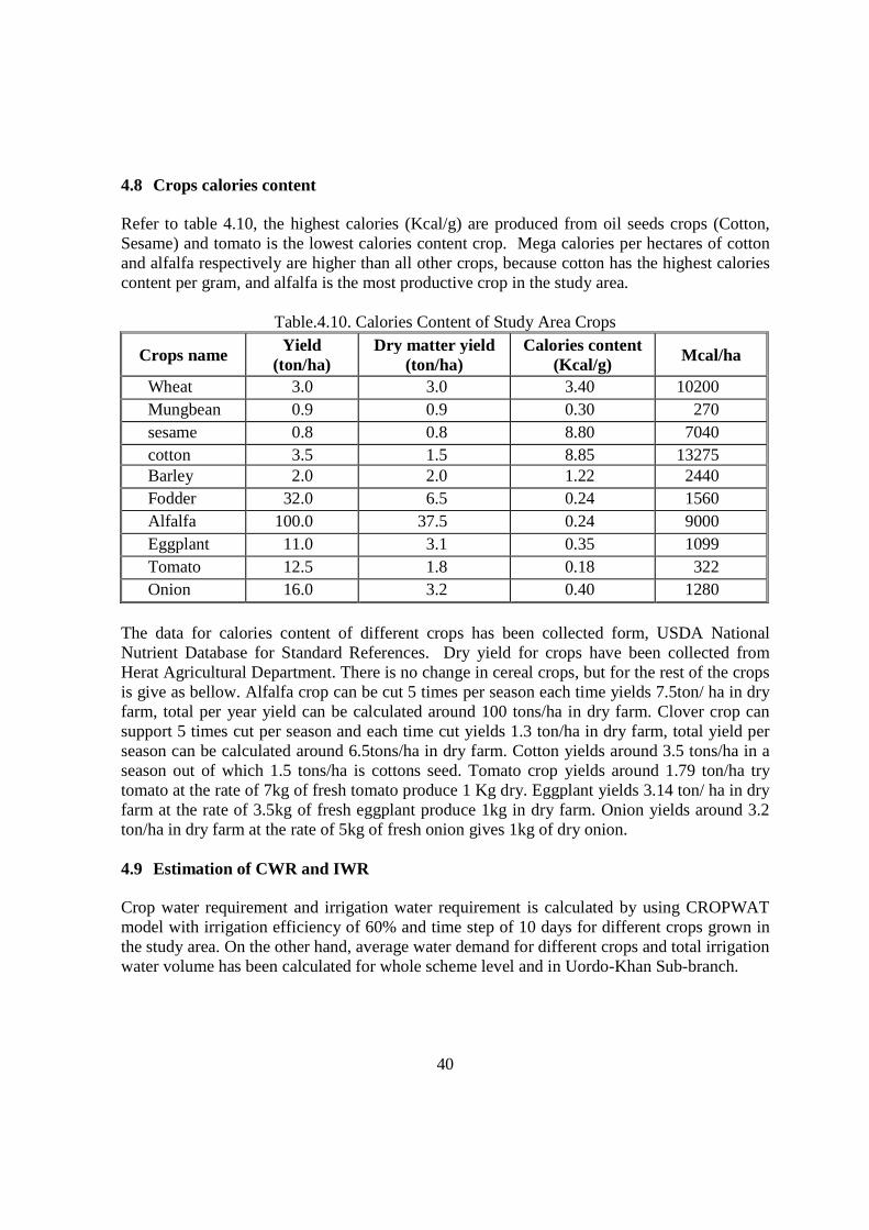
40

4.8 Crops calories content

Refer to table 4.10, the highest calories (Kcal/g) are produced from oil seeds crops (Cotton, Sesame) and tomato is the lowest calories content crop. Mega calories per hectares of cotton and alfalfa respectively are higher than all other crops, because cotton has the highest calories content per gram, and alfalfa is the most productive crop in the study area.

Table.4.10. Calories Content of Study Area Crops

Crops name Yield

(ton/ha) Dry matter yield

(ton/ha) Calories content

(Kcal/g) Mcal/ha

Wheat 3.0 3.0 3.40 10200 Mungbean 0.9 0.9 0.30 270 sesame 0.8 0.8 8.80 7040 cotton 3.5 1.5 8.85 13275 Barley 2.0 2.0 1.22 2440 Fodder 32.0 6.5 0.24 1560 Alfalfa 100.0 37.5 0.24 9000 Eggplant 11.0 3.1 0.35 1099 Tomato 12.5 1.8 0.18 322 Onion 16.0 3.2 0.40 1280

The data for calories content of different crops has been collected form, USDA National Nutrient Database for Standard References. Dry yield for crops have been collected from Herat Agricultural Department. There is no change in cereal crops, but for the rest of the crops is give as bellow. Alfalfa crop can be cut 5 times per season each time yields 7.5ton/ ha in dry farm, total per year yield can be calculated around 100 tons/ha in dry farm. Clover crop can support 5 times cut per season and each time cut yields 1.3 ton/ha in dry farm, total yield per season can be calculated around 6.5tons/ha in dry farm. Cotton yields around 3.5 tons/ha in a season out of which 1.5 tons/ha is cottons seed. Tomato crop yields around 1.79 ton/ha try tomato at the rate of 7kg of fresh tomato produce 1 Kg dry. Eggplant yields 3.14 ton/ ha in dry farm at the rate of 3.5kg of fresh eggplant produce 1kg in dry farm. Onion yields around 3.2 ton/ha in dry farm at the rate of 5kg of fresh onion gives 1kg of dry onion. 4.9 Estimation of CWR and IWR

Crop water requirement and irrigation water requirement is calculated by using CROPWAT model with irrigation efficiency of 60% and time step of 10 days for different crops grown in the study area. On the other hand, average water demand for different crops and total irrigation water volume has been calculated for whole scheme level and in Uordo-Khan Sub-branch.

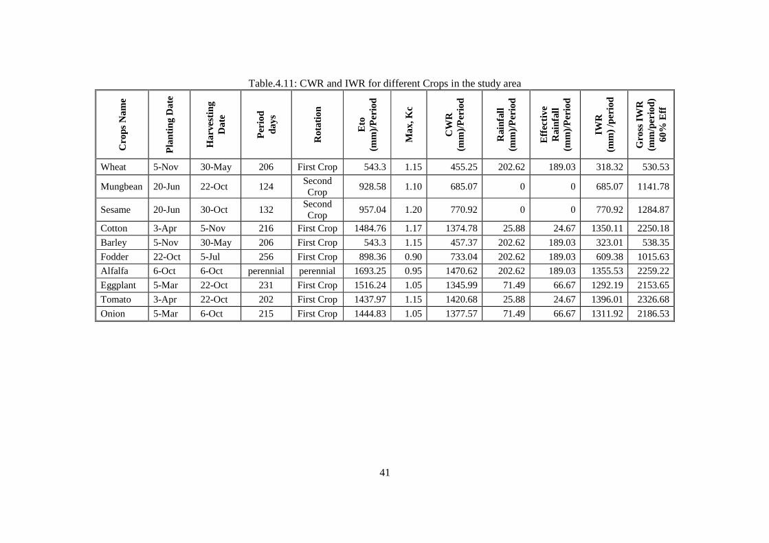
41

Table.4.11: CWR and IWR for different Crops in the study area

Cro

ps N

ame

Pla

ntin

g D

ate

Har

vest

ing

Dat

e

Per

iod

da

ys

Rot

atio

n

Eto

(m

m)/

Per

iod

Max

, Kc

CW

R

(m

m)/

Per

iod

Rai

nfal

l

(m

m)/

Per

iod

Eff

ecti

ve

Rai

nfal

l

(mm

)/P

erio

d

IWR

(m

m)

/per

iod

Gro

ss I

WR

(m

m/p

erio

d)

60%

Eff

Wheat 5-Nov 30-May 206 First Crop 543.3 1.15 455.25 202.62 189.03 318.32 530.53

Mungbean 20-Jun 22-Oct 124 Second Crop

928.58 1.10 685.07 0 0 685.07 1141.78

Sesame 20-Jun 30-Oct 132 Second Crop

957.04 1.20 770.92 0 0 770.92 1284.87

Cotton 3-Apr 5-Nov 216 First Crop 1484.76 1.17 1374.78 25.88 24.67 1350.11 2250.18

Barley 5-Nov 30-May 206 First Crop 543.3 1.15 457.37 202.62 189.03 323.01 538.35

Fodder 22-Oct 5-Jul 256 First Crop 898.36 0.90 733.04 202.62 189.03 609.38 1015.63

Alfalfa 6-Oct 6-Oct perennial perennial 1693.25 0.95 1470.62 202.62 189.03 1355.53 2259.22

Eggplant 5-Mar 22-Oct 231 First Crop 1516.24 1.05 1345.99 71.49 66.67 1292.19 2153.65

Tomato 3-Apr 22-Oct 202 First Crop 1437.97 1.15 1420.68 25.88 24.67 1396.01 2326.68

Onion 5-Mar 6-Oct 215 First Crop 1444.83 1.05 1377.57 71.49 66.67 1311.92 2186.53

42

Fig.4.13: Comparison of CWR, IWR, ETo, and Effective rainfall for whole crops

Refer to (fig.4.13) it shows that wheat and barley which are occupied respectively 50 and 12 % of the case study land area, consuming the minimum water respectively 318.3 and 323.01 mm, due to low CWR and high effective rainfall in the study area. Alfalfa has the highest water consumption than others, because it has the longest age than all others, which is calling (Perennial crop). All vegetable crops (Eggplant, Tomato, and, Onion), are almost having similar irrigation requirement. The water requirement for these crops is higher because of high evapotranspiration and less effective rainfall during their age period. Oil seed crops (Cotton, and Sesame), irrigation requirement for these two crops is totally different because of difference in their cultivable time, cotton is cultivated in 3th of April, but sesame is a second crop which is normally cultivated after harvesting wheat and barley in 20 June. Herewith, cotton required more irrigation than sesame. Table.4.12 indicates that total net irrigation requirement for entire Jui-Naw scheme and Urodo-Khan sub branch respectively are 19.75 Million m3 and 1.66 Million m3.

43

Table.4.12: Water quantity for entire Jui-Naw irrigation system and & Uordo-Khan branch

44

Table.4.13: Impact of irrigation efficiency on GIR

Table 4.13 shows the impact of irrigation efficiency on IWR for different crops. Improvement in efficiency by 10% could result to save as average 21.4 % of GIR of different crops. The water required for mungbean in 60% irrigation efficiency is equal to 1141.78 mm/period, but if irrigation efficiency improves to 70 % the water requirement for mungbean fall down to 978.67. It means 14.29 % of required ware could be saved. The techniques to save water through improving irrigation efficiency is the appropriate way to save water to expand the irrigated land, or else the saved water could be used for other economical users aspect.

45

Table 4.14 accordingly shows the extra land area that could be covered for each crop; of course the crop which need less water could extend in a high coverage than the crop required more water.

Table.4.14 Extra land for different crops based on efficiency improvement

Crops Name Total Area (ha)

Required water for total area

(m3)

Available water due to efficiency

improvement (m3)

extendable land based on

available water (ha)

Mungbean 27 184680 39576.92 5.79 sesame 15 115566 24765.79 3.21 cotton 12 161772 34667.74 2.57 Alfalfa 6 81449.4 17454.61 1.29 Eggplant 9 116082 24876.37 1.93 Tomato 9 125442 26882.22 1.93 Onion 9 117882 25262.11 1.93 Total 87 1,659,611 193, 485.76

46

4.10 Comparison of farmers strategies with the actual condition

The best way for examine farmer’s strategies against the actual crop water need for practiced crops is to explore monthly total gross irrigation requirement for all practiced crops and then compare them with monthly canal water supply. Result of this scenario count the scarcity of available water versus actual crops irrigation requirements. The water demand for different crops is derived with the help of CROPWAT model with a time step of 30 days. Table.4.15 is indicating monthly base field water demand for different crops. Total gross irrigation requirement is calculated with respect to an overall irrigation efficiency of 60 %.

Table.4.15. Monthly net IWR and total gross IWR for practiced crops in the study Area (mm) Crops Name Oct Nov Dec Jan Feb Mar Apr May Jun Jul Aug Sep Total

IWR (mm)

Wheat - 26.38 0 0 1.65 51.11 135.72 103.09 - - - - 318 Mungbean 31 - - - - - - - 35.81 163.08 260.6 194.55 685 sesame 71.14 - - - - - - - 53.72 154.62 275.93 215.51 771 cotton 83.74 - - - - - 27.36 106.68 233.71 316.02 377.07 205.57 1350 Barley - 13.28 0 0 1.65 51.11 146.45 110.52 - - - - 323 Fodder 13.94 23.33 0 0 0 45.28 129.81 200.56 196.46 - - - 609 Alfalfa 70.65 17.99 0 0 0 34.02 118.46 202.68 245.58 256.33 230.57 178.86 1355 Eggplant 89.01 - - - - 0 39.88 154.22 261.61 284.54 260.5 202.44 1292 Tomato 44.82 - - - - - 64.02 154.04 257.89 311.74 370.58 192.93 1396 Onion 20.29 - - - - 15.21 87.56 190.88 266.77 284.54 260.5 186.16 1312 Net IWR /month

424.6 80.98 0 0 3.3 196.7 749.26 1222.67 1551.6 1770.87 2035.8 1376.02 9412

Gross IWR/month

707.6 135 0 0 5.5 327.9 1248.8 2037.8 2585.9 2951.45 3392.9 2293.37 15686

47

To understand the actual field situation, table 4.15 is multiplied with the cropped area in Uordo- khan canal; of course field cropping intensity is considered as well. Table 4.16 is depicting net required quantity of water in different months in the study area and total monthly gross quantity of water with respect to 60 % irrigation efficiency.

Table.4.16: Actual monthly water requirement of different crops in the study area (m3)

Crops Name

Net cultivated area(m2)

Crop area (%)

Oct Nov Dec Jan Feb Mar Apr May Jun Jul Aug Sep Total IWR (m3)

Wheat

3,000,000

50 - 39600 0 0 2475 76650 203550 154500 - - - - 476775 Mungbean 9 8370 - - - - - - - 9720 44010 70200 52380 184680 sesame 5 10671 - - - - - - - 8055 23190 41250 32400 115566 cotton 4 10044 - - - - - 3288 12720 27960 37920 45240 24600 161772 Barley 12 - 4788 0 0 594 18396 52560 39600 - - - - 115938 Fodder 9 3753 6291 0 0 0 12231 34830 54000 52920 - - - 164025 Alfalfa 2 4590 1079 0 0 0 2040 7080 12120 14700 15360 13800 10680 81449 Eggplant 3 8010 - - - - 0 3582 13860 23490 25560 23400 18180 116082 Tomato 3 4032 - - - - - 5760 13860 23220 27990 33300 17280 125442 Onion 3 1827 - - - - 1368 7884 17100 24003 25560 23400 16740 117882 Total 3,000,000 100 51297 51758 0 0 3069 110685 318534 317760 184068 199590 250590 172260 1,659,611 Total monthly Gross Flow

Rate with 60% Irr efficiency 85,495 86,264 0 0 5115 184475 530,890 529,600 306,780 332,650 417,650 287,100 2,766,019

Total irrigable area* Cropping intensity = Net cultivated area, Total Case Study Area= 400 ha, Cropping Intensity = 75 %, Hence, Net cultivated area = 400*0.75= 300 ha, Total Gross Irrigation Flow Rate = Total monthly IWR (m3) / Irrigation Efficiency

48

Table.4.17. Comparison of the monthly available canal flow with gross irrigation requirement Months Oct Nov Dec Jan Feb Mar Apr May Jun Jul Aug Sep

Monthly Net field water

Demand (m3)51297 51758.4 0 0 3069.0 110685 318534 317760 184068 199590 250590 172260

Monthly Gross field

Water Demand (m3)85495 86264 0 0 5115.0 184475 530890 529600 306780 332650 417650 287100

Monthly Canal

Available Water (m3) 177497.6 171771.8 267304.3 357298.6 322721.3 640994.7 894862 924691 510080 129474 129474 148522

RWS 2.08 1.99 _ _ 63.1 3.47 1.69 1.75 1.66 0.39 0.31 0.52 Table.4.17 is presenting the summary of Table 4.16 and canal monthly available water, that is calculated on account of a rectangular weir, according Francis’s formula for different seasons and months, net IWR that is derived monthly based with the help of CROPWAT model, and gross IWR, which is calculated with respect of 60% of overall irrigation efficiency.

Fig.4.14. Comparison of current irrigation water supply and demand in the study area

Figure.4.14 describes clearly the water shortages during July, August, and September for the crops that are cultivated after May in the study area. August has the highest water shortages than July and September. In August the gross irrigation water demand for all practiced crops in the study area is (0.417Million m3), but the canal flow rate is (0.129 Million m3), which is showing 69 % water deficit than what is required to be supplied for the practiced crops. Figure 4.15 illustrates the comparison of effective rainfall Vs, evapotranspiration in the area of study that is depicting some valid reason of water shortage in the canal during the observed months. High temperature during summer, low rainfall, and high evapotranspiration are the major cause of this shortage.

49

Fig.4.15: Comparison of Rainfall, Effective Rainfall and Evapotranspiration

Thus, according to current demand and supply it is proofed that, farmers are not able to make satisfy their cropped lands demand with the available canal supply. Though, farmer’s approaches seem correct in case of water shortage to bring down cropping intensity, it means do not cultivate all available area therefore, current cropping intensity is fallen down to 75% by the farmers. But still farmers do not know the optimal situation with respect to the available resources, current results indicates that famers are accepting unknown yield reduction in their fields. The next objectives of this study give the optimal cropping system options in account of different scenarios. 4.11 Cropping System Scenarios

To quantify the possible cropping system three scenarios are considered. • Reducing area of all crops towards optimal supply of water, and IWR satisfaction, • Eliminating some crops towards optimal supply of water, and IWR satisfaction,

and last • keeping all crops but with sub-optimal supply of water

4.11.1 Reducing Area of All Crops and Optimal Supply of Water

The general idea is that water should be utilized optimally to maximize the net benefits and satisfy the calories demand with respect to the supply and demand. The first step is considered for finding the sensitive stage of all the crops faced water shortages during the age of the crops. Hence, by using the result from Figure 4.14 it is clear that all the practiced crops, which are cultivated after May are facing shortfall during July, August and September.

50

The aim of the first scenario is to reduce the cropped area to some extent to all for being able to satisfy the demand with the available supply. With consideration of relative water supply the land is allocated as shown in table 4.18. Moreover, the maximum total monthly crops water demand is derived here from table, 4.17 and then divided by the 60 % irrigation efficiency to gain monthly gross income.

Table.4.18 Land allocation with the calculation of RWS, to maximize NB & Cal. outcome

RWS = ∑ Min, Water Supply/ Max, Demand = 129473.9 /427450 = 0.303 Land Allocation for Mungbean based on RWS= 0.303*27= 8.18 ha Net income and calories content calculation of practiced crop respectively referred to table (4.9) and (4.10). According to the result in (Table.4.18), the overall area is reduced in a very high extent from 87 hectare to 26.35 hectare, which indicates an overall 69.7% area reduction due to water availability limitation, and the remaining land are allocated to the crops back along with the consideration of available water. Result of new land allocation for the practiced crops is tested with respect to the net income and calories production as well. The overall net income and calories production can be gained with this scenario respectively are USD52623.69 and 106112.73 mega calories. Mungbean which is the only crop occupying more land than all others shows a very less income and calories production due to the other crops. But among all the practiced crops cotton and alfalfa are showing significant high economic return and calories production in their area of cultivation. 4.11.2 Eliminating Some Crops and Optimal Supply of Water

The main concept of second scenario is to eliminate some crops, to adjust the current land according the available water supply. Optimization technique is used to maximize net economic return (NER), calories production, and to minimize the fertilizer and labor under limited water supply for identifying the cropping system options. Linear programming is used to model scenarios to allocate the available resource like, water, land, labor, irrigation, and

51

fertilizer in the best possible manner so to gain maximum profit. Two scenarios have been developed for maximization, and two for minimization to help for the right decision in the study area. Quantitative System for Business (Win-QSB), which is an optimization technique tool that use simplex algorithm, has been used to help for the problem solution. The scenarios bellow are modeled such as, constraints imposed on the objective function to be incorporate components that account for farmers preference important on the area of cultivation.

• Maximizing the net economic return (NER) based on the resource availability. • Maximizing the calories producing due to available constraint. • Minimizing the fertilizers for different crops kilograms per hectares. • Minimize the labor force per hectare of the cultivated lands.

Bellow table 4.19 shows all resource availability and limitation for the crops in the study area. Gross irrigation water requirement (m3/month/ ha) for each crop is selected based on maximum demand of water in months of July, August and September.

Table.4.19 Resource availability and limitation for all the crops in study area

The objective function of the model for maximizing the net income is formulated based on all crops cultivated in the study area.

Z = ∑NBiXi Where, NBi = Net benefits from Xi i = 1, 2… 7 Let x1 = cultivable area (ha) for Mungbean Let x2 = cultivable area (ha) for Sesame Let x3 = cultivable area (ha) for Cotton Let x4 = cultivable area (ha) for Alfalfa Let x5 = cultivable area (ha) for Eggplant

52

Let x6 = cultivable area (ha) for Tomato Let x7 = cultivable area (ha) for Onion Thus, mathematically we can present the objective function as bellow

Max Z= 449.82X1 + 1776.9X2 + 5242.2X3 + 5446.8X4 + 686.2X5 + 1802.2X6 + 1883. Constraints

(1) Constraints due to irrigation water requirement (Water, M3/Month/ha): Gross irrigation water requirement should be less than or equal to the available water during the shortage period, Jul, Aug, and Sep. 4333.3X1 + 4583.3X2+ 6283.3X3 + 4266.7X4+ 4733.3X5+ 6166.7X6+4733.3 X7 <= 129473.9

(2) Constraint due to fertilizer requirement of each crop (Kg/ha): Fertilizer requirement should be greater or equal to the total land available multiply to the minimum fertilizer which is used to any crop. (87*65= 5655). It shows that 65 ha cultivated by mungbean require 5655Kg of fertilizers which is the minimum requirement than other crops in the study area. 65X1 + 100X2 + 250X3 + 150X4+ 220X5 + 250X6 + 300X7 >= 5655

(3) Constraint due to labor requirement of each crop (Person/ha): It should be greater or equal to the total land available multiply by the minimum labor requirement for a crop the minimum labor.(87*10=870 ), it means if we cultivate the total land area with mungbean crop 870 person is required ,which is the less labor work on the field than the other crops, so 10X1 + 15X2 + 50X3 + 65X4+ 40X5 + 45X6+ 75X7 >= 870

(4) Constraint due to seed requirement of each crops (Kg/ha): It should be greater or equal to the total land available multiply by the minimum crop seed which is required, (87*0.25=22), it means if we cultivate the total land area with eggplant, 22Kg seed is required ,which is the less seed than the other crops, so 15X1 + 6X2+ 14X3 + 20X4+ 0.25X5+ 0.3X6 + 15X7 >= 22

(5) Constraint due to irrigation labor requirement of each crop (Person/ha): It should be greater or equal to the total land available multiply by the irrigation labor for a crop which requires minimum number of labor.(87*5=435 person), it means if we cultivate the total land area by the mungbean crop 435 person is required, that is the less number of labor than the other crops irrigation labor requirement , so 5X1 + 7X2 + 20X3 + 30X4 + 16X5 + 20X6 + 35X7 >= 435

53

(6) Constraint due to land availability for each crop (ha): The sum of cropped area cannot X1 + X2+ X3 + X4+ X5+ X6+ X7 +X13 <= 87

(7) Constraints due to calories production (Mcal/ha): It should be greater or equal to the total available land multiply by the multiplier of a crop which is produced minimum calories, (87*270=23490), it means if we cultivate the total land area with mungbean crop than 23490 mega calories would be produced, which is the lowest calories production compare to other crops. 270X1 + 7040X2 + 13275X3 + 9000X4 + 1099X5 + 322.2X6 + 1280X7>= 23490

(8) Non-negative constraints: The model has applied different value for the land until it reached to an optimal one, herewith all crops land area should be greater or equal to the zero. X1, X2, X3, X4, X5, X6, X7 >= 0

The bellow result in table (4.20) shows that, for adjusting the highest economic return and calories production it is required to keep 21.1 ha alfalfa, 8.3ha onion, out of 87 ha, and the rest all should be eliminated from the copping system. The net benefits and calories production in this scenario is showing 40.18 % and 52.73% respectively increment than the first scenario (Reducing area of all crops towards optimal supply of water).

54

Table.4.20: Land allocation, with respect to give up crops to gain max NB Decision Solution Unit Cost or Total Reduced Basis Allowable AllowableVariable Value Profit c(j) Contribution Cost Status Min. c(j) Max. c(j)

Mungbean 0 449.8 0 -7800.96 at bound _ M 8250.76Sesame 0 1776.9 0 -5977.06 at bound _ M 7753.96Alfalfa 21.18 5446.8 115386.5 0 basic 3925.27 MCotton 0 5242.2 0 -1872.93 at bound _ M 7115.14

Eggplant 0 686.2 0 -3687.8 at bound _ M 4374Tomato 0 1802.2 0 -5036.48 at bound _ M 6838.68Onion 8.26 1883.6 15554.5 0 basic -6713.6 6042.45

Objective Function (Max.) = 130941

Left Hand Right Hand Slack Shadow Allowable AllowableConstraint Side Direction Side or Surplus Price Min. RHS Max. RHS

fertilizer 5655 >= 5655 0 -31.13 4551.78 8206.15seed 547.55 >= 22 525.55 0 _ M 547.55

Calories 201229 >= 23490 177739 0 _ M 201228.6C.Labor 1996.32 >= 870 1126.32 0 _ M 1996.32I. Labor 924.55 >= 435 489.55 0 _ M 924.55Water 129474 <= 129473.9 0 2.37 89222.7 160854.6Land 29.44 <= 87 57.56 0 29.44 M

(Right Hand Side) is showing the limit resource which was defined for each crop, but (Left hand Side) is indicating the optimal situation according to the constraint, maximum calories can be produced from this scenario is listed in (Left Hand Side) equal to 201229 mega calories. Furthermore, surplus values are showing the difference between left and right side. The shadow price is showing that 2.37 unit of water can increase one more unit land under the cultivation. One scenario is developed only for the crops which direct fulfill food requirements. Table 4.21 indicates that, the only crop can give the maximum income whenever to eliminate alfalfa and cotton is onion, to allocate 27.35 ha land out of 87ha for onion the maximum outcome could be achieved that is USD 51523.68. A reduction of 39.35 % in maximum net income and 17.4 % in calories production would occur than the first scenario that is given in Table 4.20.

55

Table.4.21: Land allocation, without consideration of (Alfalfa and Cotton) to max NB Decision Solution Unit Cost or Total Reduced Basis Allowable AllowableVariable Value Profit c(j) Contribution Cost Status Min. c(j) Max. c(j)

Mungbean 0 449.8 0 -1274.62 at bound _ M 1724.421Sesame 0 1776.9 0 -47.008 at bound _ M 1823.908Eggplant 0 686.2 0 -1197.4 at bound _ M 1883.6Tomato 0 1802.2 0 -651.817 at bound _ M 2454.017Onion 27.3538 1883.6 51523.68 0 basic 1835.054 M

Objective Function (Max.) = 51523.68

Left Hand Right Hand Slack Shadow Allowable AllowableConstraint Side Direction Side or Surplus Price Min. RHS Max. RHS

fertilizer 8206.15 >= 5655 2551.15 0 _ M 8206.15seed 410.3075 >= 22 388.308 0 _ M 410.3075

Calories 35012.91 >= 23490 11522.9 0 _ M 35012.91C.Labor 2051.538 >= 870 1181.54 0 _ M 2051.538I. Labor 957.3842 >= 435 522.384 0 _ M 957.3842Water 129473.9 <= 129473.9 0 0.3979 89222.7 411797.1Land 27.3538 <= 87 59.6462 0 27.3538 M

The first scenario was the indicator of maximum calories production as well as net income with the consideration of all cropping system. Thus one more scenario is developed for calories maximization in the study area without consideration of alfalfa and cotton to prioritize the crops which direct fulfill people food requirements. Following the mathematical form of this scenario is written bellow. Z = ∑Cal Xi Where, Cali = calories produced form Xi i = 1, 2… 7 Max Z=270X1 + 7040X2 + 13275X3 + 9000X4 + 1099X5 + 322.2X6 + 1280X7 All constraint would be the same as NER scenario just here instead NB calorie is replaced, and NB objective function will take place as a constraint.

56

Table.4.22: Land allocation, without consideration of (Alfalfa and cotton) to max calories Decision Solution Unit Cost or Total Reduced Basis Allowable AllowableVariable Value Profit c(j) Contribution Cost Status Min. c(j) Max. c(j)

Mungbean 0 270 0 -7,285.66 at bound _ M 7,555.66Sesame 13.3924 7,040.00 94,282.25 0 basic 1,239.44 MEggplant 0 1,099.00 0 -2,617.02 at bound _ M 3,716.02Tomato 0 322.2 0 -5,634.35 at bound _ M 5,956.55Onion 14.3859 1,280.00 18,413.92 0 basic -3,130.62 7,270.40

Objective Function (Max.) = 112,696.20

Left Hand Right Hand Slack Shadow Allowable AllowableConstraint Side Direction Side or Surplus Price Min. RHS Max. RHS

fertilizer 5,655.00 >= 5,655.00 0 -30.4503 4,505.62 8,206.15seed 296.1424 >= 22 274.1424 0 _ M 296.1424

Net income 50,894.13 >= 39,132.60 11,761.53 0 _ M 50,894.13C.Labor 1,279.83 >= 870 409.8264 0 _ M 1,279.83I. Labor 597.2523 >= 435 162.2523 0 _ M 597.2523Water 129,473.90 <= 129,473.90 0 2.2004 98,709.19 233,971.30Land 27.7782 <= 87 59.2218 0 27.7782 M

The result for this scenario has given above in table 4.22 that indicates without cotton and alfalfa, the highest calories achieve whenever to allocate 13.39 ha to sesame and 14.39 ha out of 87ha area. The calorie production goes down in study area because cotton and alfalfa contributes high calories to the cropping system. To remove alfalfa and cotton 56 % deduction would be arise than the scenario has been developed with all crops, which is given in table 4.20. To allocate the available lands to the crops which are using the minimum fertilizer, a minimization model has been developed; bellow is the mathematical expression of the model.

Z = ∑FiXi Where, Fi = Fertilizer required for Xi i = 1, 2… 7 Min Z= 65X1 + 100X2 + 250X3 + 150X4+ 220X5 + 250X6 + 300X7

The constraints for this scenario are similar to the previous one; merely fertilizer is moved as an objective function and the rest all are presented as constraints

57

Table 4.23: Land allocation due to minimum fertilizer consumption Decision Solution Unit Cost or Total Reduced Basis Allowable AllowableVariable Value Profit c(j) Contribution Cost Status Min. c(j) Max. c(j)

Mungbean 0 65 0 40 at bound 25 MSesame 0 100 0 65 at bound 35 MAlfalfa 14.5 150 2175 0 basic 0 257.1429Cotton 0 250 0 150 at bound 100 M

Eggplant 0 220 0 140 at bound 80 MTomato 0 250 0 150 at bound 100 MOnion 0 300 0 125 at bound 175 M

Objective Function (Min.) = 2175

Left Hand Right Hand Slack Shadow Allowable AllowableConstraint Side Direction Side or Surplus Price Min. RHS Max. RHS

Net income 78978.59 >= 39132.6 39846 0 _ M 78978.59seed 290 >= 22 268 0 _ M 290

Calories 130500 >= 23490 107010 0 _ M 130500C.Labor 942.5 >= 870 72.5 0 _ M 942.5I. Labor 435 >= 435 0 5 401.5385 910.3562Water 61867.15 <= 129473.9 67606.7 0 61867.16 MLand 14.5 <= 87 72.5 0 14.5 M

The result in table 4.23 indicates that, 2175 kilogram fertilizer is the minimum amount, whenever to allocate 14.5 ha to alfalfa crop and the rest all should be zero. Same scenario has been developed without alfalfa and cotton to minimize the fertilizer usage in the area of study based on the available constraints. The result is shown in table 5.24.

58

Table 4.24: Land allocation due to minimum fertilizer, without (Cotton and alfalfa) Decision Solution Unit Cost or Total Reduced Basis Allowable AllowableVariable Value Profit c(j) Contribution Cost Status Min. c(j) Max. c(j)

Mungbean 0 65 0 16.9803 at bound 48.0197 MSesame 11.2287 100 1122.866 0 basic 60 211.5645Eggplant 0 220 0 87.8529 at bound 132.1471 MTomato 0 250 0 57.8353 at bound 192.1647 MOnion 10.1828 300 3054.852 0 basic 106.0048 423.6463

Objective Function (Min.) = 4177.718

Left Hand Right Hand Slack Shadow Allowable AllowableConstraint Side Direction Side or Surplus Price Min. RHS Max. RHS

Net income 39132.6 >= 39132.6 0 0.0286 24975.22 50610.5seed 220.1145 >= 22 198.1145 0 _ M 220.1145

Calories 92083.8 >= 23490 68593.8 0 _ M 92083.8C.Labor 932.1429 >= 870 62.1429 0 _ M 932.1429I. Labor 435 >= 435 0 7.034 406 727.1401Water 99662.74 <= 129473.9 29811.15 0 99662.74 MLand 21.4115 <= 87 65.5885 0 21.4115 M

To allocate in order 11.23 ha and 10.18 ha respectively to sesame and onion the minimum fertilizer requirements would be achieved, which is 4177.72kilograms. The first scenario with consideration of alfalfa and cotton is showed 52.06 % reduction than this scenario. For allocating the available lands to the crops that are using the minimum labor for the crops, a minimization model has been developed; bellow is the mathematical expression of the model.

Z = ∑CLXi Where, CLi = Crops labor required for Xi i = 1, 2… 7 Min Z= 10X1 + 15X2 + 50X3 + 65X4+ 40X5 + 45X6+ 75X7

For this scenario all constraints are similar to the pervious scenarios, just here crops labor requirement is changed to objective function and the rest all demonstrated as constraint. The result in table (4.25) which is given bellow, shows that, to minimize the labor force for the crops, out of 87 ha land is allocated to 1.7 ha, 15.8 ha, and 5.1 ha respectively for sesame, tomato and onion and the minimum solution for this scenarios is 1119.8 person

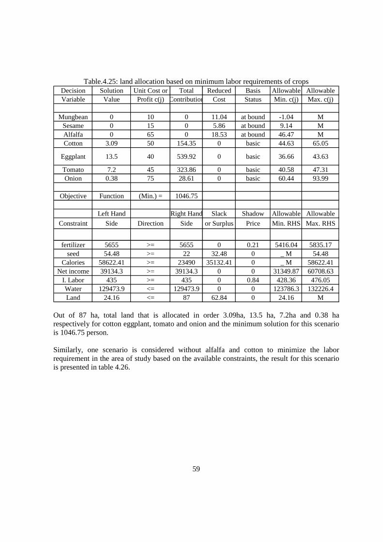
59

Table.4.25: land allocation based on minimum labor requirements of crops Decision Solution Unit Cost or Total Reduced Basis Allowable AllowableVariable Value Profit c(j) Contribution Cost Status Min. c(j) Max. c(j)

Mungbean 0 10 0 11.04 at bound -1.04 MSesame 0 15 0 5.86 at bound 9.14 MAlfalfa 0 65 0 18.53 at bound 46.47 MCotton 3.09 50 154.35 0 basic 44.63 65.05

Eggplant 13.5 40 539.92 0 basic 36.66 43.63

Tomato 7.2 45 323.86 0 basic 40.58 47.31Onion 0.38 75 28.61 0 basic 60.44 93.99

Objective Function (Min.) = 1046.75

Left Hand Right Hand Slack Shadow Allowable Allowable

Constraint Side Direction Side or Surplus Price Min. RHS Max. RHS

fertilizer 5655 >= 5655 0 0.21 5416.04 5835.17seed 54.48 >= 22 32.48 0 _ M 54.48

Calories 58622.41 >= 23490 35132.41 0 _ M 58622.41Net income 39134.3 >= 39134.3 0 0 31349.87 60708.63

I. Labor 435 >= 435 0 0.84 428.36 476.05Water 129473.9 <= 129473.9 0 0 123786.3 132226.4Land 24.16 <= 87 62.84 0 24.16 M

Out of 87 ha, total land that is allocated in order 3.09ha, 13.5 ha, 7.2ha and 0.38 ha respectively for cotton eggplant, tomato and onion and the minimum solution for this scenario is 1046.75 person. Similarly, one scenario is considered without alfalfa and cotton to minimize the labor requirement in the area of study based on the available constraints, the result for this scenario is presented in table 4.26.

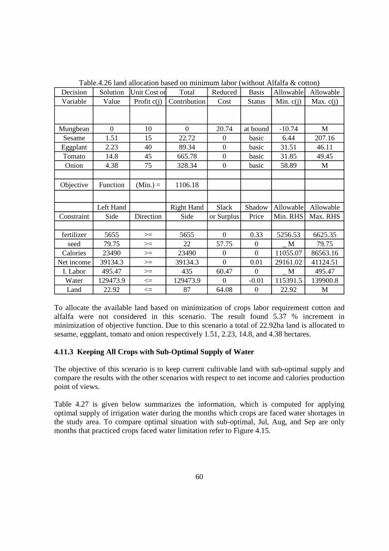
60

Table.4.26 land allocation based on minimum labor (without Alfalfa & cotton) Decision Solution Unit Cost or Total Reduced Basis Allowable AllowableVariable Value Profit c(j) Contribution Cost Status Min. c(j) Max. c(j)

Mungbean 0 10 0 20.74 at bound -10.74 MSesame 1.51 15 22.72 0 basic 6.44 207.16Eggplant 2.23 40 89.34 0 basic 31.51 46.11Tomato 14.8 45 665.78 0 basic 31.85 49.45Onion 4.38 75 328.34 0 basic 58.89 M

Objective Function (Min.) = 1106.18

Left Hand Right Hand Slack Shadow Allowable AllowableConstraint Side Direction Side or Surplus Price Min. RHS Max. RHS

fertilizer 5655 >= 5655 0 0.33 5256.53 6625.35seed 79.75 >= 22 57.75 0 _ M 79.75

Calories 23490 >= 23490 0 0 11055.07 86563.16Net income 39134.3 >= 39134.3 0 0.01 29161.02 41124.51

I. Labor 495.47 >= 435 60.47 0 _ M 495.47Water 129473.9 <= 129473.9 0 -0.01 115391.5 139900.8Land 22.92 <= 87 64.08 0 22.92 M

To allocate the available land based on minimization of crops labor requirement cotton and alfalfa were not considered in this scenario. The result found 5.37 % increment in minimization of objective function. Due to this scenario a total of 22.92ha land is allocated to sesame, eggplant, tomato and onion respectively 1.51, 2.23, 14.8, and 4.38 hectares. 4.11.3 Keeping All Crops with Sub-Optimal Supply of Water

The objective of this scenario is to keep current cultivable land with sub-optimal supply and compare the results with the other scenarios with respect to net income and calories production point of views. Table 4.27 is given below summarizes the information, which is computed for applying optimal supply of irrigation water during the months which crops are faced water shortages in the study area. To compare optimal situation with sub-optimal, Jul, Aug, and Sep are only months that practiced crops faced water limitation refer to Figure 4.15.

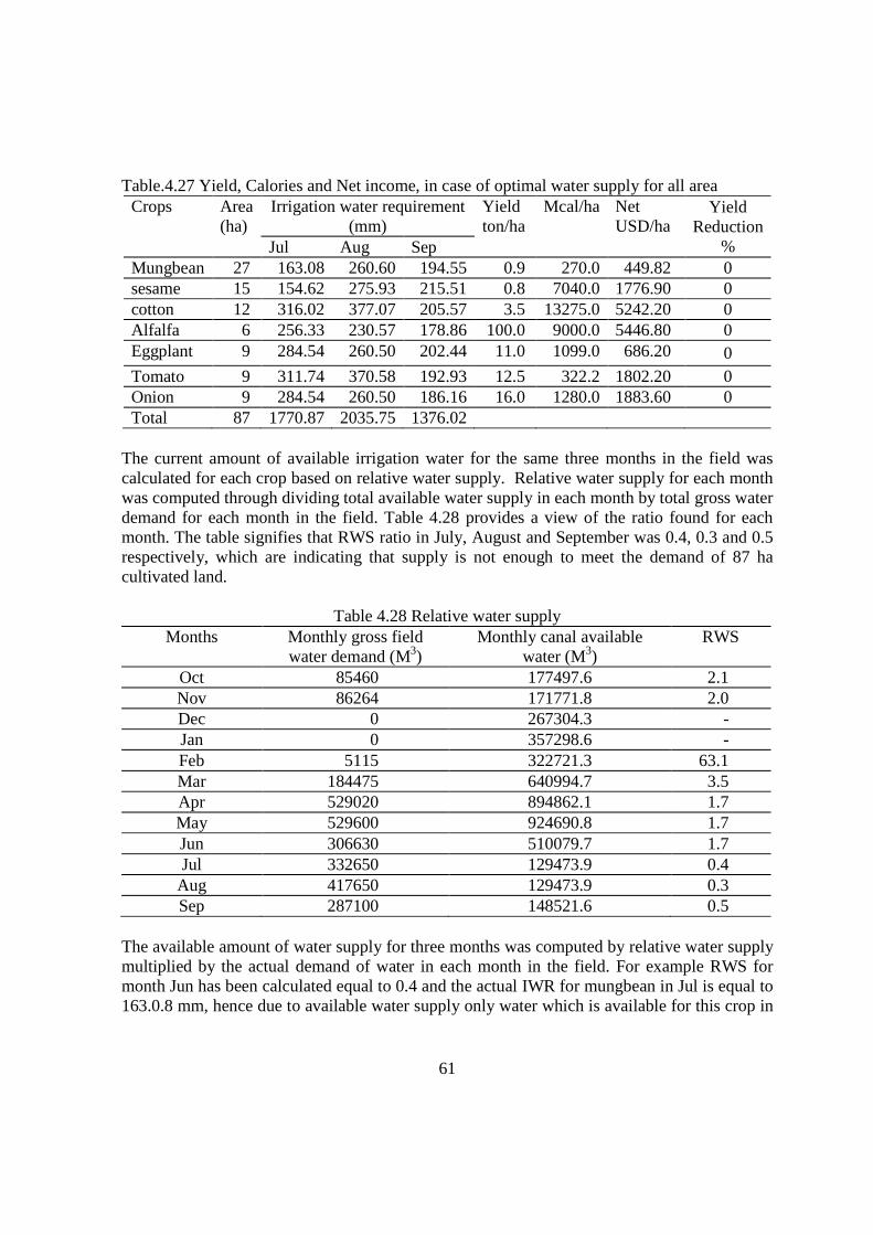
61

Table.4.27 Yield, Calories and Net income, in case of optimal water supply for all area Crops Area

(ha) Irrigation water requirement

(mm) Yield ton/ha

Mcal/ha Net USD/ha

Yield Reduction

% Jul Aug Sep Mungbean 27 163.08 260.60 194.55 0.9 270.0 449.82 0 sesame 15 154.62 275.93 215.51 0.8 7040.0 1776.90 0 cotton 12 316.02 377.07 205.57 3.5 13275.0 5242.20 0 Alfalfa 6 256.33 230.57 178.86 100.0 9000.0 5446.80 0 Eggplant 9 284.54 260.50 202.44 11.0 1099.0 686.20 0 Tomato 9 311.74 370.58 192.93 12.5 322.2 1802.20 0 Onion 9 284.54 260.50 186.16 16.0 1280.0 1883.60 0 Total 87 1770.87 2035.75 1376.02

The current amount of available irrigation water for the same three months in the field was calculated for each crop based on relative water supply. Relative water supply for each month was computed through dividing total available water supply in each month by total gross water demand for each month in the field. Table 4.28 provides a view of the ratio found for each month. The table signifies that RWS ratio in July, August and September was 0.4, 0.3 and 0.5 respectively, which are indicating that supply is not enough to meet the demand of 87 ha cultivated land.

Table 4.28 Relative water supply Months Monthly gross field

water demand (M3) Monthly canal available

water (M3) RWS

Oct 85460 177497.6 2.1 Nov 86264 171771.8 2.0 Dec 0 267304.3 - Jan 0 357298.6 - Feb 5115 322721.3 63.1 Mar 184475 640994.7 3.5 Apr 529020 894862.1 1.7 May 529600 924690.8 1.7 Jun 306630 510079.7 1.7 Jul 332650 129473.9 0.4 Aug 417650 129473.9 0.3 Sep 287100 148521.6 0.5

The available amount of water supply for three months was computed by relative water supply multiplied by the actual demand of water in each month in the field. For example RWS for month Jun has been calculated equal to 0.4 and the actual IWR for mungbean in Jul is equal to 163.0.8 mm, hence due to available water supply only water which is available for this crop in

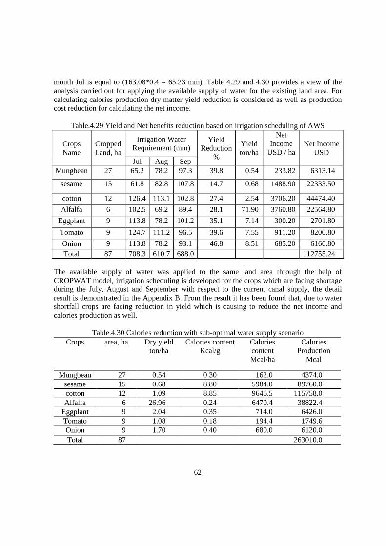
62

month Jul is equal to (163.08*0.4 = 65.23 mm). Table 4.29 and 4.30 provides a view of the analysis carried out for applying the available supply of water for the existing land area. For calculating calories production dry matter yield reduction is considered as well as production cost reduction for calculating the net income.

Table.4.29 Yield and Net benefits reduction based on irrigation scheduling of AWS

Crops Name

Cropped Land, ha

Irrigation Water Requirement (mm)

Yield Reduction

%

Yield ton/ha

Net Income

USD / ha Net Income

USD Jul Aug Sep

Mungbean 27 65.2 78.2 97.3 39.8 0.54 233.82 6313.14

sesame 15 61.8 82.8 107.8 14.7 0.68 1488.90 22333.50

cotton 12 126.4 113.1 102.8 27.4 2.54 3706.20 44474.40

Alfalfa 6 102.5 69.2 89.4 28.1 71.90 3760.80 22564.80

Eggplant 9 113.8 78.2 101.2 35.1 7.14 300.20 2701.80

Tomato 9 124.7 111.2 96.5 39.6 7.55 911.20 8200.80

Onion 9 113.8 78.2 93.1 46.8 8.51 685.20 6166.80 Total 87 708.3 610.7 688.0 112755.24

The available supply of water was applied to the same land area through the help of CROPWAT model, irrigation scheduling is developed for the crops which are facing shortage during the July, August and September with respect to the current canal supply, the detail result is demonstrated in the Appendix B. From the result it has been found that, due to water shortfall crops are facing reduction in yield which is causing to reduce the net income and calories production as well.

Table.4.30 Calories reduction with sub-optimal water supply scenario Crops area, ha Dry yield

ton/ha Calories content

Kcal/g Calories content Mcal/ha

Calories Production

Mcal

Mungbean 27 0.54 0.30 162.0 4374.0 sesame 15 0.68 8.80 5984.0 89760.0 cotton 12 1.09 8.85 9646.5 115758.0 Alfalfa 6 26.96 0.24 6470.4 38822.4

Eggplant 9 2.04 0.35 714.0 6426.0 Tomato 9 1.08 0.18 194.4 1749.6 Onion 9 1.70 0.40 680.0 6120.0 Total 87 263010.0

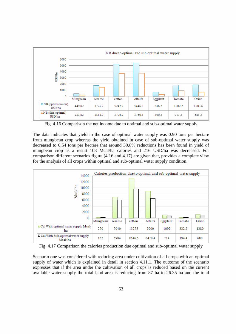
63

Fig. 4.16 Comparison the net income due to optimal and sub-optimal water supply

The data indicates that yield in the case of optimal water supply was 0.90 tons per hectare from mungbean crop whereas the yield obtained in case of sub-optimal water supply was decreased to 0.54 tons per hectare that around 39.8% reductions has been found in yield of mungbean crop as a result 108 Mcal/ha calories and 216 USD/ha was decreased. For comparison different scenarios figure (4.16 and 4.17) are given that, provides a complete view for the analysis of all crops within optimal and sub-optimal water supply condition.

Fig. 4.17 Comparison the calories production due optimal and sub-optimal water supply

Scenario one was considered with reducing area under cultivation of all crops with an optimal supply of water which is explained in detail in section 4.11.1. The outcome of the scenario expresses that if the area under the cultivation of all crops is reduced based on the current available water supply the total land area is reducing from 87 ha to 26.35 ha and the total

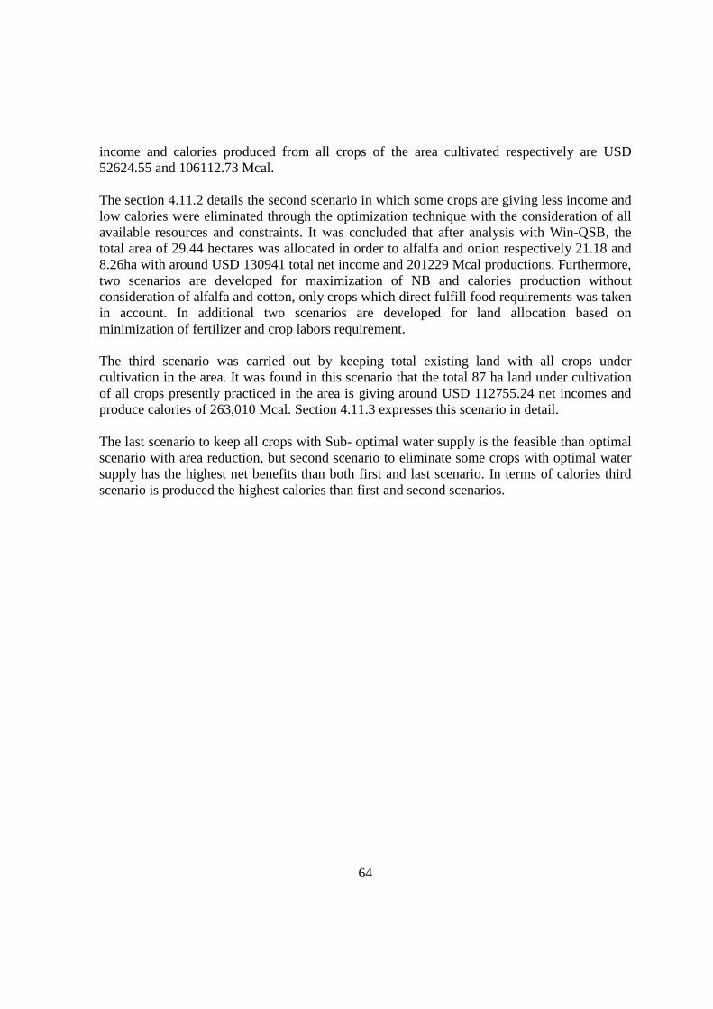
64

income and calories produced from all crops of the area cultivated respectively are USD 52624.55 and 106112.73 Mcal. The section 4.11.2 details the second scenario in which some crops are giving less income and low calories were eliminated through the optimization technique with the consideration of all available resources and constraints. It was concluded that after analysis with Win-QSB, the total area of 29.44 hectares was allocated in order to alfalfa and onion respectively 21.18 and 8.26ha with around USD 130941 total net income and 201229 Mcal productions. Furthermore, two scenarios are developed for maximization of NB and calories production without consideration of alfalfa and cotton, only crops which direct fulfill food requirements was taken in account. In additional two scenarios are developed for land allocation based on minimization of fertilizer and crop labors requirement. The third scenario was carried out by keeping total existing land with all crops under cultivation in the area. It was found in this scenario that the total 87 ha land under cultivation of all crops presently practiced in the area is giving around USD 112755.24 net incomes and produce calories of 263,010 Mcal. Section 4.11.3 expresses this scenario in detail. The last scenario to keep all crops with Sub- optimal water supply is the feasible than optimal scenario with area reduction, but second scenario to eliminate some crops with optimal water supply has the highest net benefits than both first and last scenario. In terms of calories third scenario is produced the highest calories than first and second scenarios.

65

CHAPTER 5

CONCLUSION AND RECOMMENDATION

5.1 Conclusion

This study investigates cropping system options in context of irrigation water scarcity. It aims at improving irrigation water allocation with the objectives of maximizing net economic return and calories production, and minimizing selected production factors. CWR and IWR for all practiced crops are estimated for the study area based on local climatic and cropping system information. Current field situation, as per farmers’ practices and water availability, is quantified in terms of demand and supply, and compared with the actual crop water needs. Different scenarios are tested including different possible cropping systems under optimal and sub-optimal water supply. Current farmers’ strategy consists in keeping all crops under deficit irrigation and area reduction due to water limitation, and all scenarios are compared for selecting the best option for maximizing NER and Cal production. The CROPWAT model is used to determine CWR and IWR for all practiced crops in the study area. The gross irrigation requirement is calculated on the basis of different irrigation efficiencies with 10-day time step in the study area for all practiced crops. Results show that 10% improvement in irrigation efficiency result in saving average 21.4% GIR for each practiced crop in the area. Consequently different size of irrigated land area can be expanded for different crops. Comparison of the farmers crop planning and actual water availability has been done with the help of CROPWAT model and canal flow estimation on monthly basis through field observation, result shows relative water supply (RWS) for July, August, and September are 0.4, 03, and 0.5 respectively, which indicates 60, 70, and 50% water shortage in same months for those crops grown after May. The reasons for water shortage are high evapotranspiration and lack of rainfall at that time. Possible adjustments of cropping system are investigated through different scenarios:

• Reducing area of all crops towards optimal supply of water, and IWR satisfaction, • Eliminating some crops towards optimal supply of water, and IWR satisfaction, • Keeping all crops but with sub-optimal supply of water (deficit irrigation, as practiced

by farmers).

In the first scenario, areas of all crops are reduced proportionally by 30.3 % to adjust the overall supply to meet the amalgamated demand. The maximum net benefit and Cal outcome of this scenario are USD 52,625, and 106,113 Mcal respectively.

66

The second scenario is implemented through linear programming as an optimization technique that uses simplex algorithm, to identify the cropping system option, through the maximization of net economic return (NER), calories production, and minimization of fertilizer and crop labor requirements. The last scenario tries to investigate the strategy implemented by farmers through deficit irrigation on all crops and to inquire its outcome. Irrigation scheduling is developed for the crops which are facing shortage during the July, August, and September with respect to the current canal supply. The results indicate that due to water shortfall crops are facing reduction in yield which is inducing to reduce the net income and calories production as well in the study area. Results show that second scenario (elimination of some crops and optimal water supply) is providing 13.89% and 59.8 % higher net economic return than first and third scenarios which are respectively,

� Reducing area of all crops towards optimal supply of water and � Keeping all crops but with sub-optimal supply of water

But the highest calorie output results are from third scenario which show 23.5% higher calorie outcome than the scenario which provides highest NER. To allocate land based on minimum fertilizer requirement with the consideration of only crops which directly fulfill food requirement, sesame and onion are the only crops which are occupying the land with the minimum fertilizer requirements. Moreover, for allocating the land based on minimum labor requirement, sesame, eggplant, tomato and onion are the crops which are allocated with the minimum labor requirement. The overall finding of this study can be used to support the decision making and result demonstrate good guidelines for the planners; it can be helpful for farmer to take decision on adjustment of their cropping system according their demand (Max NER, Max Cal). Study shows that reduction in area of all crops and deficit irrigation are not the best options due to lower NER. Higher calorie is produced by keeping all crops with sub-optimal water supply, which obviously helps for food security. The study provides means for achieving higher NER, optimal irrigation supply for selective cropping system and less diversification with the limited water availability. Understanding of CWR, IWR, and the irrigation scheduling during the shortage months help farmers to take the right decision for preventing any yield reduction in their farm. And more finding would be applicable for other places in the country with similar climatic condition.

67

5.2 Recommendation

For making the study more effective the following should be taken in account,

� For better optimizing cropping system a study should focus on the other similar schemes with more detailed analysis of cropping systems with respect to farming style, different strategies to ascertain who use alternative sources (GW), who can reduce land and who extend the land, and explore farmers calorie demand from each crop.

� Though CROPWAT model provides reasonable estimates of CWR and IWR, for more reliable results it should be validated in context of study area

� The government’s and NGO’s subsidies for farmers to change their traditional irrigation

system to more efficient system like drip and sprinkle irrigation, would improve the farmer NER and calories contribution.

� Water resource management aspect should be improved to alleviate losses to prevent water

shortage in the study area.

68

REFERENCES

Aini, A. (2007). Water Conservation in Afghanistan. Rural Engineering Coordinator Swedish Committee for Afghanistan (SCA) Journal of Developments in Sustainable Agriculture, 2: 51-58 (2007)

Asad, S.Q. (2002). Water Resources Management in Afghanistan: The Issues and Options

(WORKING PAPER 49) IWMI, Pakistan Country Series No. 14 ADB (2008). Preparing the Water Resources Development Project. Technical Assistance

Report, Project Number: 42091, Islamic Republic of Afghanistan April, 2008. ADB (2005), Asian Development Bank, Islamic Republic of Afghanistan: Western Basins,

Water Resources Management and Irrigated, Agriculture Development Project, Technical Assistance Consultant’s Report, Project Number: 36252, July 2005.

Amir Kassam, Smith, M. (2001). FAO Methodologies on Crop Water Use and Crop Water

Productivity, Expert meeting on crop water productivity, Rome, 3 to 5 December 2001. Paper no cwp-m07

Beutler, A.M., Keller, A.A. (2005). Implementation of FAO-56 Penman-Monteith

Evapotranspiration in a Large Scale Irrigation Scheduling Program. American Society of Civil Engineers (Apr 21, 2005)

Burt, C.M. 1999. Irrigation Water Balance Fundamentals. Conference on Benchmarking

Irrigation System Performance Using Water Measurement and Water Balances. San Luis Obispo, CA. March 10. USCID, Denver, Colo. pp. 1-14

Cranfield University (2007). Improving irrigation water use efficiency. Irrigation scheduling

using water balance http://www.ukia.org FAO (1996). Corporate Document Report, Irrigation Scheduling: from Theory to Practice –

Proceedings. Theme 6: social, cultural, institutional and policy constraints. Irrigation scheduling in a developing country: Experiences from Tamil Nadu, India

Forouda, E. H. Hobbsa, R. Rieweb and T. Entz.( 1992). Field verification of a microcomputer

irrigation model. Agricultural Water Management, 21(3): 215-234 FAO (1998). Food and Agriculture Organization of the United Nations, Crop

evapotranspiration guidelines for computing crop water requirements - FAO Irrigation and drainage paper 56, Rome, 1998.

69

Georgea. B. A. Shendeb. S.A. and Raghuwanshi N. S (2000). Development and testing of an irrigation scheduling model, Agricultural Water Management, 46 (2): 121-136.

ICARDA (2002). International Center for Agricultural Research in the Dry Area. Need

Assessment on Soil and Water in Afghanistan, Sponsored by the United States Agency for International Development. Aleppo, Syria (2002)

Jamshid Yarahmadi (2003). The Integration of Satellite Image, GIS and CROPWAT model to

Investigation of water balance in Irrigation area. Johl,S (1979). Irrigation and agriculture Development. United National Based on the

International Expert Consultation, Iraq. Hossein Arsham (1994). Computer-assisted Learning Concepts & Techniques. (Computer

Implementations with the WinQSB Package). Ministry of Energy & Water (2007). Water Sector Strategy for Afghanistan national

development strategy (with focus on prioritization) Modoi. P.N, Seth. S.M. Hydraulics & Fluid Mechanics. Published by Rajinder Kumar Jain,

thirteenth edition (2000). Chapter- 10, pp (464-470) Rout, B. (2008). Water management, livestock and the opium economy, How the Water

Flows: A Typology of Irrigation Systems in Afghanistan. Afghanistan Research and Evaluation Unit Issue Paper Series

Raphy Favre and Golam Monowar Kamal, (2004). Watershed atlas of Afghanistan (IST

edition - working document for planners), kabul: fao/faahm-undp/aims, (2003) Smajstrla, A.G., B.J. Boman, D.Z. Haman, F.T. Izuno, D.J. Pitts, and F.S. Zazueta. 2006.

Basic Irrigation Scheduling in Florida. http://edis.ifas.ufl.edu/AE111. Accessed 7 November, 2006

Smajstrla A.G. and. Zazueta F.S (2002).Estimating Crop Irrigation Requirements for Irrigation

System Design and Consumptive Use Permitting, Institute of Food and Agricultural Sciences, University of Florida, Gainesville, 32611

Sheng-Feng Kuo1, Bor-Jang Lin2 and Horng-Je Shieh (2001). CROPWAT model to evaluate

crop water requirements in Taiwan. 1 st. Asian Regional Conference. Seoul, 2001

70

Suat Irmak and Dorota Z. Haman (2003). Evapotranspiration: Potential or Reference? Florida Cooperative Extension Service, Institute of Food and Agricultural Sciences, University of Florida. Original publication date: June 2003. http://edis.ifas.ufl.edu

Singh.D. K. Jaiswal C. S. Reddy K. S. , Singh R. M. and Bhandarkar D. M (2001). Optimal

cropping pattern in a canal command area. Agricultural Water Management, 50(1):1-8, August 2001

Snyder R.L, Orang.M, Bali. K, Eching. S (2002). Basic Irrigation Scheduling, Retrieved on

April 2007. University of California Tollefson L.C. and Wahab M.N.J (2008). Agriculture and Agri-Food Canada, Better

Research-Extension-Farmer Interaction can improve the Impact of Irrigation Scheduling Techniques

UN-Water (2006). Coping with water scarcity. A strategic issue and priority for system-wide

action. ftp://ftp.fao.org/agl/aglw/docs/waterscarcity.pdf United State Department of Agriculture (USDA). National Nutrient Database for Standard

Reference, Release 20. (Content of Selected Foods per Common Measure, sorted alphabetically Energy kcal)

World Water Day (2007) Coping with water scarcity, Challenge of the twenty- first century http://www.fao.org/nr/water/docs/escarcity.pdf

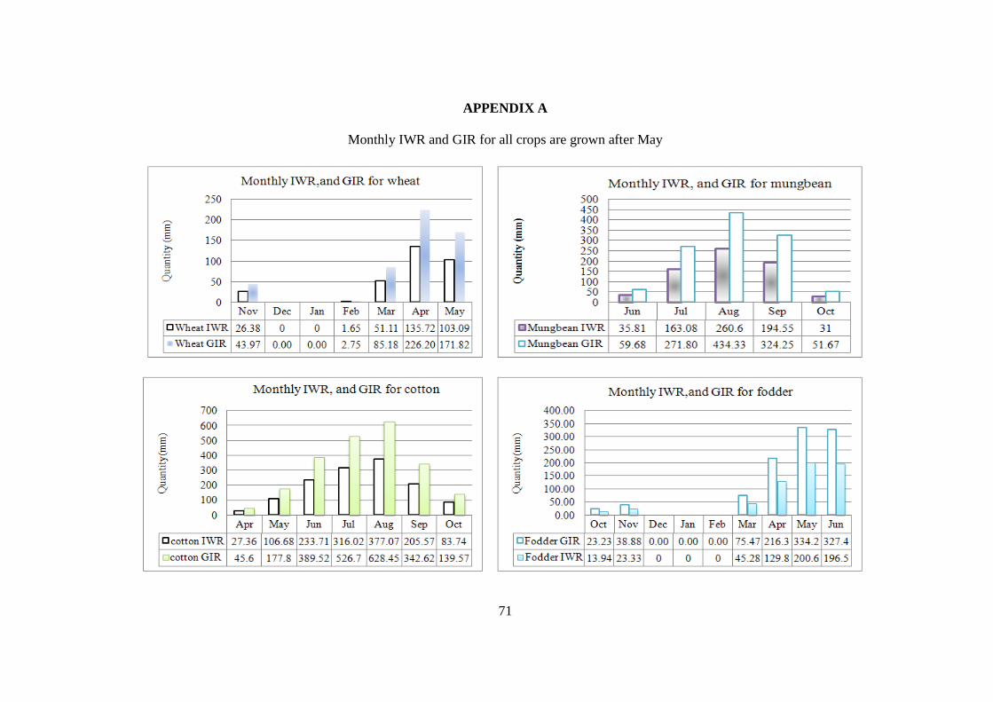
71

APPENDIX A

Monthly IWR and GIR for all crops are grown after May

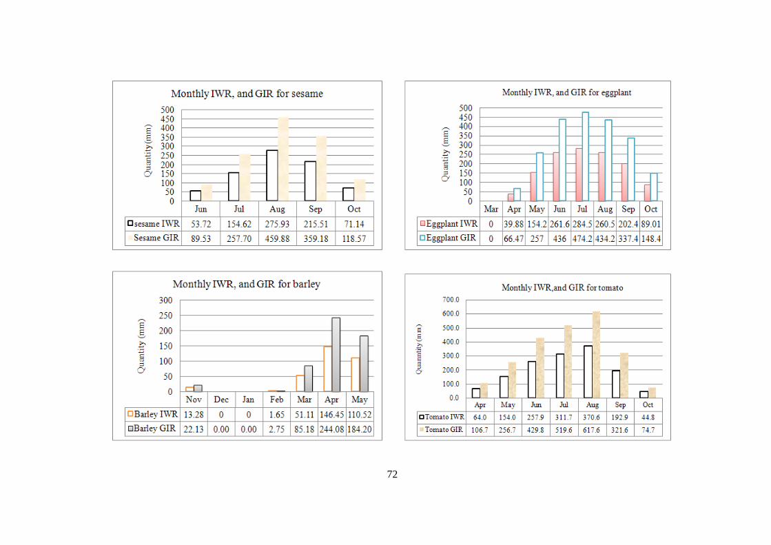
72

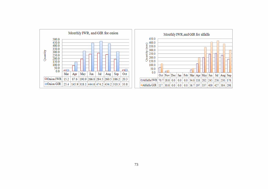
73

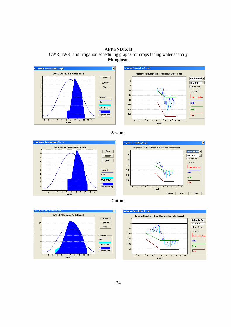
74

APPENDIX B CWR, IWR, and Irrigation scheduling graphs for crops facing water scarcity

Mungbean

Sesame

Cotton

75

Alfalfa

Eggplant

Tomato

76

Onion

77

APPENDIX C Table C-1 Mean monthly wind speed in Herat – Afghanistan

Years Oct Nov Dec Jan Feb Mar Apr May Jun Jul Aug Sep2008 NA NA NA 3 6 7 6 6 NA NA 15 92007 5 NA NA 5 6 6 6 11 11 18 16 132006 5 5 4 4 6 5 5 10 17 20 18 82005 5 5 4 4 6 5 5 10 17 20 18 82004 NA NA NA NA 6 5 7 7 14 15 16 132003 14 7 4 5 7 8 5 8 12 16 18 112002 6 NA 5 5 8 7 6 7 10 16 18 10

Mean monthly wind Speed (2002-2008)

7 5 4 4 6 6 6 8 13 17 17 10

Table C-2 Mean monthly Sunshine in Herat – Afghanistan

Years Oct Nov Dec Jan Feb Mar Apr May Jun Jul Aug Sep2008 NA NA NA 5:11 7:49 6:37 7:45 12:21 NA NA 11:41 10:182007 9:27 NA NA 6:42 6:03 6:10 7:57 11:50 11:16 12:00 11:59 10:582006 NA 6:30 NA 5:05 5:35 5:50 7:33 8:21 8:45 8:42 NA NA2005 8:53 7:16 6:40 6:49 5:44 6:05 8:11 10:24 10:47 10:46 10:10 9:342004 NA NA NA NA 8:12 7:29 NA NA NA 12:03 12:11 7:402003 10:08 6:54 NA 5:11 6:44 7:01 8:51 11:35 11:18 11:37 11:52 NA2002 NA NA NA 6:11 6:39 8:20 7:54 NA NA NA NA NA2001 8:25 6:53 4:07 NA NA NA NA NA NA NA NA NA

Average Sunshine hours (2001-2008)

9:13 6:53 5:23 5:51 6:41 6:47 8:02 10:54 10:31 11:01 11:35 9:38

78

Table C-3 Mean monthly humidity in Herat – Afghanistan Years Oct Nov Dec Jan Feb Mar Apr May Jun Jul Aug Sep1942 30 52 66 74 64 60 55 35 27 22 24 261943 65 76 88 NA 71 72 59 60 NA NA NA 561944 45 58 61 87 91 80 73 65 46 43 34 371945 37 56 69 72 70 65 68 55 35 29 30 301946 38 53 59 64 62 60 60 44 30 22 26 301947 42 63 78 59 63 57 57 54 35 27 27 281948 57 61 70 78 73 59 62 47 53 NA NA 461949 57 61 76 81 73 67 52 41 42 40 50 561951 49 49 46 66 75 50 55 36 34 33 38 381952 40 52 68 69 71 59 68 51 39 22 14 221955 44 62 84 57 61 54 49 50 34 30 29 301956 43 58 54 82 72 64 60 52 45 44 50 561958 41 45 56 70 55 70 63 46 44 41 22 281959 34 51 53 62 66 59 59 34 21 22 21 211960 39 48 74 79 67 71 50 44 37 29 32 321961 27 30 59 70 61 59 46 35 28 24 19 291962 32 45 69 78 80 64 57 37 27 29 26 351963 40 46 72 71 67 59 60 44 31 28 26 321964 48 51 71 83 73 67 62 50 30 27 26 331965 43 60 62 82 61 59 54 38 26 23 26 251966 32 67 60 68 65 54 44 38 27 23 20 211967 36 41 64 67 64 58 43 34 23 17 21 221968 31 79 60 73 79 63 53 42 35 28 34 351969 47 47 57 68 64 59 51 44 34 35 34 371970 47 74 76 71 73 74 51 39 31 31 36 331971 51 50 63 70 66 61 63 50 41 37 41 451972 39 56 73 70 62 58 47 40 32 21 26 341973 38 49 72 72 59 59 49 36 30 27 28 271974 35 40 46 47 56 51 47 39 32 28 21 221975 61 46 45 34 35 42 37 29 22 26 24 371976 41 NA NA 64 61 59 55 64 55 38 40 432001 34.9 46.9 48.8 54.8 44.2 46.5 45.1 34.0 24.1 NA NA 31.82002 51.8 53.7 75.9 64.2 66.3 52.7 57.4 51.6 35.1 NA NA 40.02003 44.5 56.9 67.8 63.8 56.0 55.4 53.6 47.2 34.7 28.4 26.8 35.12004 NA NA 63.8 NA 44.1 45.6 NA NA NA 37.1 31.8 37.72005 54.0 63.2 60.0 72.1 73.2 73.1 69.3 59.7 51.1 39.4 41.1 43.12006 49.1 60.0 67.8 71.7 61.5 58.8 54.3 48.9 33.3 33.5 28.8 39.72007 55.3 NA NA 59.8 66.0 61.1 56.0 45.2 37.8 31.9 29.4 33.2

Average of (1942-1976) 42.2 54.2 65.0 69.6 66.5 61.1 55.1 44.3 34.2 29.2 29.1 33.7Average of (19421-2007) 43.2 54.5 64.9 68.8 65.1 60.2 55.3 44.8 34.5 29.9 29.5 34.4

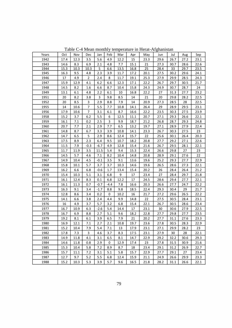
79

Table C-4 Mean monthly temperature in Herat-Afghanistan Years Oct Nov Dec Jan Feb Mar Apr May Jun Jul Aug Sep

1942 17.4 12.3 3.5 5.6 4.9 12.2 15 23.3 29.6 26.7 27.2 23.1

1943 14.6 8.3 6.9 2.1 4.8 7.7 15.1 21 27.3 30.7 28.6 22.6

1944 15.3 10.3 10.3 5 6.6 13.5 16.8 25 28.4 33 29.7 23.5

1945 16.3 9.5 4.8 2.3 3.9 11.7 17.2 20.1 27.5 30.2 29.6 24.1

1946 17 4.9 2 2.4 8 11.7 19.1 25.3 27.9 29.9 28.5 24.3

1947 15.9 12.9 4.1 6.2 6.6 12.3 17.1 22.2 26.7 29.7 30.5 21.7

1948 14.5 8.2 1.6 6.6 8.7 10.4 15.8 24.3 24.9 30.7 28.7 24

1949 13.1 6.1 4.8 2.2 6.1 10 16.8 22.2 27 31.3 27.7 23.2

1951 20 8.2 3.8 3 9.8 8.5 14 21 20 29.8 28.2 22.5

1952 20 8.5 3 2.9 8.8 7.9 14 20.9 27.3 28.5 28 22.5

1955 14 10.6 7 5.5 7.7 10.8 14.1 26.4 29 28.9 29.5 23.1

1956 17.9 10.6 7 3.1 6.1 8.7 16.6 22.2 23.5 30.3 27.5 23.9

1958 15.2 3.7 6.2 5.5 6 12.5 11.1 20.7 27.1 29.3 26.6 22.1

1959 16.1 7.1 0.2 2.5 3 9.9 18.7 21.2 26.8 28.7 29.3 24.8

1960 20.7 7.7 2.1 2.9 7.7 6.5 13.2 19.7 27.1 28.9 27.9 22.4

1961 14.8 8.7 6.7 3.3 3.9 10.8 14.1 23.3 26.7 30.3 27.5 23

1962 14.7 6.5 5 2.9 8.6 12.4 15.7 22 25.6 30.1 26.4 20.3

1963 17.5 8.9 2.3 6.4 9.5 10.7 18.2 20.8 27.7 29.2 27.1 22.6

1964 11.5 7.9 -0.3 -6.7 4.9 12.8 15.4 21.6 26.7 29.5 28.1 22.1

1965 11.7 11.9 3.5 11.5 5.4 9.4 15.3 22.4 26.6 29.8 27 23

1966 14.5 5.7 4.6 7.1 8.2 10.4 14.8 20.8 28.9 29.1 27.6 22

1967 14.9 10.4 4.5 -0.1 3.5 9.1 13.6 19.6 25.2 29.3 27.7 22.9

1968 15.8 10.1 5.7 3.7 3.7 10.3 14.6 19.6 26.5 28.6 27.3 22.1

1969 16.2 6.6 6.8 -0.6 1.7 13.4 15.4 20.2 26 28.4 26.4 21.2

1970 15.4 10.3 5.1 3.1 6.8 9 17 23.4 27 28.4 29.7 21.8

1971 16.1 12.4 8.3 0.1 6.8 12.2 17 24.5 28.6 29.4 27.7 22.1

1972 16.1 11.3 0.7 -0.7 -4.4 7.8 16.6 20.3 26.6 27.7 24.7 22.2

1973 16.3 9.1 3.4 -1.7 8.8 9.8 18.5 22.4 29.3 30.4 29 21.7

1974 12.8 8.6 3.4 0.2 0 10.2 16 21.7 27.2 29.6 26.5 22.2

1975 14.1 6.6 3.8 2.4 4.4 9.9 14.8 22 27.5 30.5 28.4 23.1

1976 16 4.9 3.7 5.7 3.2 6.8 15.4 22.1 26.7 30.5 28.6 23.4

1977 16.7 10.9 6.3 -2.6 5.4 14.4 17 23.1 30 30.6 27.9 22.5

1978 16.7 6.9 8.8 2.7 5.1 9.6 18.2 22.8 27.7 29.8 27.7 23.5

1979 19.2 8.1 6.1 3.9 6.5 7.9 21 20.2 27.7 31.1 27.6 23.3

1980 16.9 12.1 7.1 2.7 2.1 10.8 19.7 23.6 27.8 30.5 28.3 22.9

1981 15.2 10.4 7.9 5.4 7.1 13 17.9 23.1 27.1 29.9 28.2 23

1982 17.8 7.3 3 4.6 3.7 8.3 17.5 23.1 27.9 30 28 22.1

1983 14.9 11.8 4.1 3.1 6.5 8.1 14.7 22.9 29.2 32.2 30.6 29.3

1984 14.6 11.8 0.8 2.9 0 12.9 17.4 23 27.8 31.5 30.9 21.6

1985 15.3 10.4 5.8 7.2 8.9 8.7 18 23.4 29.1 31.2 26.9 22.7

1986 15.7 11.1 7.2 3.1 5.1 5.8 15.7 22.9 27.7 29.1 27 23.4

1987 12.7 9.7 5.2 5.5 6.8 12.4 15.9 21.1 24.9 26.6 29.9 23.3

1988 15.2 10.3 5.3 3.9 5.7 9.6 16.5 21.8 28.2 31.1 26.6 22.1

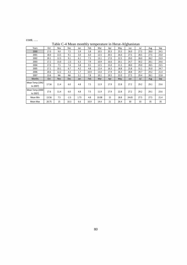
80

cont. … Table C-4 Mean monthly temperature in Herat-Afghanistan

Years Oct Nov Dec Jan Feb Mar Apr May Jun Jul Aug Sep

2000 17.0 9.0 7.5 5.9 5.8 10.5 20.3 25.5 26.0 27.5 28.0 24.5

2001 18.0 13.5 9.1 3.0 6.0 12.5 20.5 26.0 27.5 28.5 27.5 23.0

2002 20.1 12.5 9.1 6.1 7.3 13.1 17.0 22.5 29.0 28.0 28.2 23.9

2003 17.2 15.0 -2.3 6.3 7.9 10.9 16.6 20.1 24.7 30.2 28.1 24.6

2004 17.0 7.5 7.4 5.8 9.5 12.5 15.0 21.5 28.0 29.0 28.5 23.5

2005 17.1 10.1 6.7 4.2 4.8 12.4 16.3 18.8 25.8 31.1 35.0 24.7

2006 20.6 12.2 4.3 1.7 10.9 13.0 17.9 26.3 28.8 29.7 29.2 21.4

2007 13.6 NA NA 5.1 7.8 10.1 19.5 22.0 27.5 29.4 28.1 22.8

Months Oct Nov Dec Jan Feb Mar Apr May Jun Jul Aug Sep

Mean Temp (1942

to 2007)17.56 11.4 6.0 4.8 7.5 11.9 17.9 22.8 27.2 29.2 29.1 23.6

Mean Temp (2000

to 2007)17.6 11.4 6.0 4.8 7.5 11.9 17.9 22.8 27.2 29.2 29.1 23.6

Mean Min 13.56 7.5 -2.3 1.73 4.8 10.08 15 18.8 24.65 27.5 27.5 21.4

Mean Max 20.75 15 10.3 6.6 10.9 14.4 21 26.4 30 33 35 35

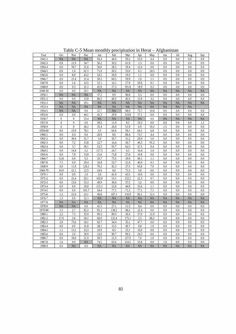
81

Table C-5 Mean monthly precipitation in Herat – Afghanistan Year Oct Nov Dec Jan Feb Mar Apr May Jun Jul Aug Sep

1941-2 NA NA NA 93.4 44.9 59.2 25.0 4.4 0.0 0.0 0.0 0.01942-3 0.8 21.9 54.7 56.2 30.2 61.9 1.3 0.0 0.0 0.0 0.0 0.01943-4 0.0 10.7 31.6 50.0 28.3 19.4 12.4 0.0 0.0 0.0 0.0 0.01944-5 0.0 1.0 61.5 71.0 20.2 33.0 6.1 24.5 0.0 0.0 0.0 0.01945-6 0.0 8.0 43.2 54.5 29.0 19.3 1.1 0.0 0.0 0.0 0.0 0.01946-7 0.0 21.4 21.4 50.2 66.5 59.9 1.0 1.1 0.0 0.0 0.0 0.01947-8 0.0 1.6 13.5 51.1 14.1 17.9 29.6 0.1 0.0 0.0 0.0 0.01948-9 0.0 9.3 31.2 45.9 27.2 101.8 18.9 0.2 0.0 0.0 0.0 0.01949-50 0.0 0.0 20.1 NA NA NA NA NA NA NA NA NA1950-1 NA NA NA 37.2 9.9 96.8 5.3 0.0 0.0 0.0 0.0 0.01951-2 0.0 0.0 15.8 86.2 49.5 45.5 12.9 3.2 0.0 0.0 0.0 0.01952-3 NA NA 29.1 NA NA NA NA NA NA NA NA NA1953-4 NA NA NA NA NA NA NA NA NA NA NA1954-5 NA NA 0.0 22.7 NA 88.9 75.7 10.6 0.0 0.0 0.0 0.01955-6 0.0 0.0 44.1 41.3 29.9 119.8 17.1 0.0 0.0 0.0 0.0 0.01956-7 0 0 33.4 NA NA NA NA 0.0 NA NA NA NA1957-8 0 0 0.0 38.5 11.0 8.5 19.2 0.0 0.0 0.0 0.0 1.21958-9 0 0 36.2 35.4 26.0 51.9 6.9 10.2 1.5 0.0 0.0 0.01959-60 0.0 23.9 78.1 3.5 64.6 59.1 64.1 6.8 0.0 0.0 0.0 0.01960-1 0.0 0.4 0.0 20.9 8.0 88.4 75.7 4.4 0.0 0.0 0.0 0.01961-2 0.0 39.4 51.7 5.0 20.7 31.2 29.0 5.0 0.0 0.0 0.0 0.01962-3 0.0 7.2 15.8 12.7 14.4 20.7 40.5 91.2 0.0 0.0 0.0 0.01963-4 0.0 3.7 30.1 23.3 95.7 62.5 37.5 0.4 0.0 0.0 0.0 0.01964-5 0.0 14.4 3.2 117.5 24.7 6.5 16.4 5.4 0.0 0.0 0.0 0.01965-6 0.0 7.8 13.8 21.6 73.8 27.6 10.8 0.0 0.0 0.0 0.0 0.01966-7 13.8 0.0 5.5 33.7 75.5 39.9 90.1 1.1 0.0 0.0 0.0 0.01967-8 7.1 0.9 39.4 26.8 53.7 31.8 40.0 6.1 0.0 0.0 0.0 0.01968-9 0.0 11.9 126.1 70.2 42.3 27.5 65.8 7.0 0.0 0.0 0.0 0.01969-70 10.9 22.1 12.5 24.0 8.0 73.3 5.0 0.0 0.0 0.0 0.0 0.01970-1 0.0 0.0 1.0 3.6 41.0 43.5 19.6 0.0 0.0 0.0 0.0 0.01971-2 0.0 21.4 20.1 102.8 53.1 152.2 22.3 9.7 0.0 0.0 0.0 0.01972-3 0.0 13.0 53.3 49.9 30.4 37.5 3.2 0.0 0.0 0.0 0.0 0.01973-4 0.0 0.0 20.8 115.1 52.6 44.9 35.6 1.1 0.0 0.0 0.0 0.01974-5 0.0 0.0 101.7 54.4 77.1 71.3 77.1 7.1 0.0 0.0 0.0 0.01975-6 1.2 22.0 23.1 49.8 107.1 110.9 85.1 12.1 0.0 0.0 0.0 0.01976-7 1.2 0.0 32.3 NA NA NA NA NA NA NA NA NA1977-8 NA NA NA NA NA NA NA NA NA NA NA NA1978-9 NA NA 0.0 41.5 27.1 11.5 9.4 0.0 0.0 0.0 0.0 0.01979-80 3.5 2.7 82.2 81.1 138.2 98.2 22.4 0.0 0.0 0.0 0.0 0.01980-1 2.2 7.5 35.9 90.5 80.0 30.4 37.0 11.9 0.0 0.0 0.0 0.01981-2 17.0 2.6 30.2 60.0 121.4 175.1 2.5 86.2 0.0 0.0 0.0 0.01982-3 2.0 73.6 54.1 62.7 34.4 35.1 47.7 0.0 0.0 0.0 0.0 0.01983-4 0.0 0.0 31.8 38.1 13.5 40.7 9.8 1.0 0.0 0.0 0.0 0.01984-5 1.1 13.1 23.3 33.9 8.5 23.1 16.0 0.0 0.0 0.0 0.0 0.01985-6 0.6 2.0 30.9 15.0 90.7 99.5 24.5 0.0 0.0 0.0 0.0 0.01986-7 0.0 18.0 21.0 50.5 21.5 127.0 7.0 1.0 0.0 0.0 0.0 0.01987-8 1.6 0.0 NA 74.5 63.4 124.5 23.8 0.0 1.0 0.0 0.0 0.01988-9 0.0 NA 0.0 NA NA NA NA NA NA NA NA NA

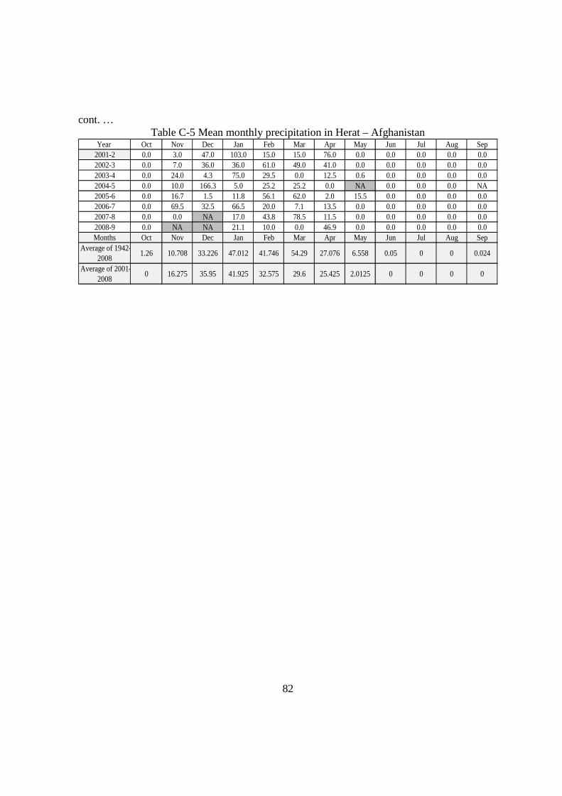
82

cont. … Table C-5 Mean monthly precipitation in Herat – Afghanistan

Year Oct Nov Dec Jan Feb Mar Apr May Jun Jul Aug Sep2001-2 0.0 3.0 47.0 103.0 15.0 15.0 76.0 0.0 0.0 0.0 0.0 0.02002-3 0.0 7.0 36.0 36.0 61.0 49.0 41.0 0.0 0.0 0.0 0.0 0.02003-4 0.0 24.0 4.3 75.0 29.5 0.0 12.5 0.6 0.0 0.0 0.0 0.02004-5 0.0 10.0 166.3 5.0 25.2 25.2 0.0 NA 0.0 0.0 0.0 NA2005-6 0.0 16.7 1.5 11.8 56.1 62.0 2.0 15.5 0.0 0.0 0.0 0.02006-7 0.0 69.5 32.5 66.5 20.0 7.1 13.5 0.0 0.0 0.0 0.0 0.02007-8 0.0 0.0 NA 17.0 43.8 78.5 11.5 0.0 0.0 0.0 0.0 0.02008-9 0.0 NA NA 21.1 10.0 0.0 46.9 0.0 0.0 0.0 0.0 0.0Months Oct Nov Dec Jan Feb Mar Apr May Jun Jul Aug Sep

Average of 1942-2008

1.26 10.708 33.226 47.012 41.746 54.29 27.076 6.558 0.05 0 0 0.024

Average of 2001-2008

0 16.275 35.95 41.925 32.575 29.6 25.425 2.0125 0 0 0 0

83

APPENDIX D

Table D-1 Crop water requirement report for wheat

84

Table D-2 Crop water requirement report for mungbean

85

Table D-3 Crop water requirement report for sesame

86

Table D-4 Crop water requirement report for cotton

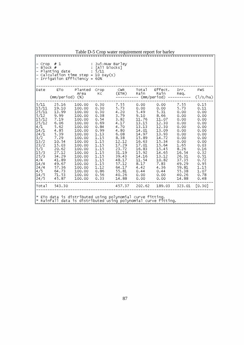
87

Table D-5 Crop water requirement report for barley

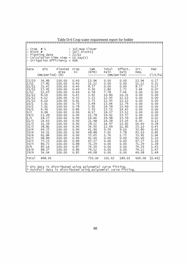
88

Table D-6 Crop water requirement report for fodder

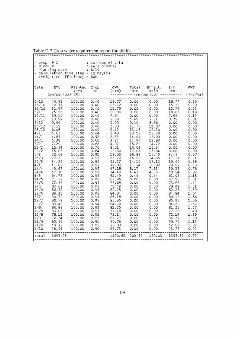
89

Table D-7 Crop water requirement report for alfalfa

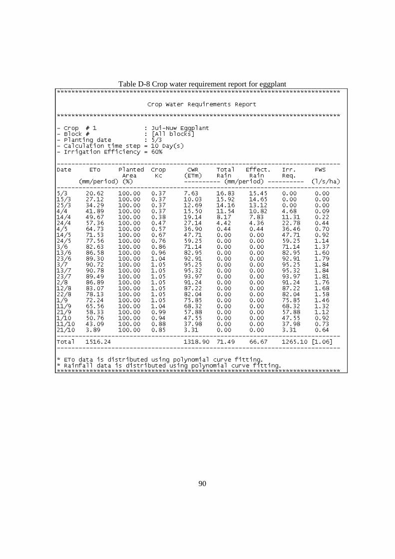
90

Table D-8 Crop water requirement report for eggplant

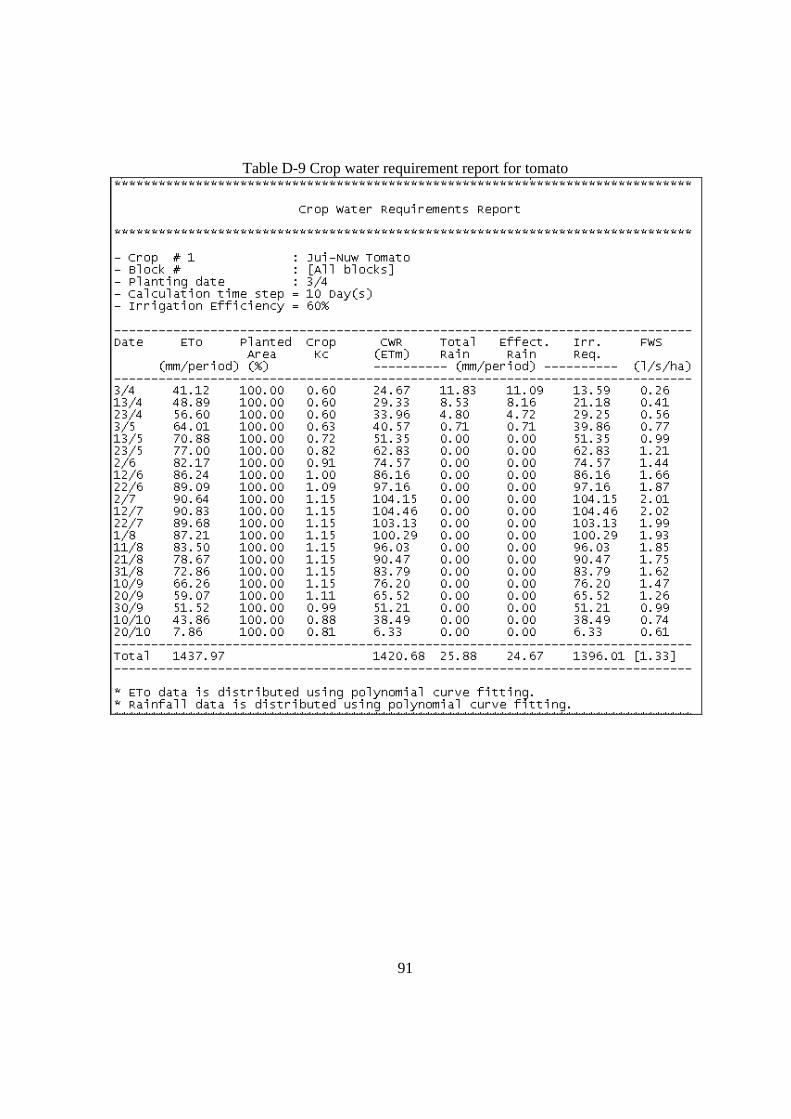
91

Table D-9 Crop water requirement report for tomato

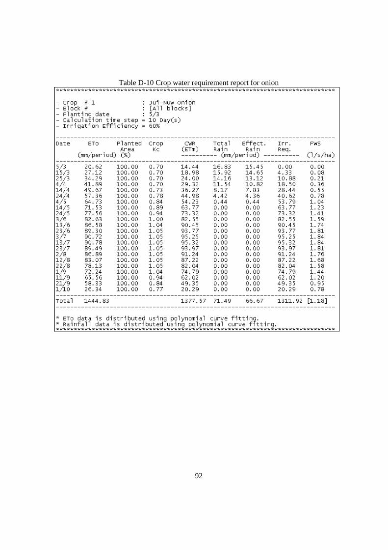
92

Table D-10 Crop water requirement report for onion

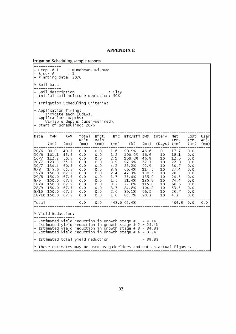
93

APPENDIX E Irrigation Scheduling sample reports

94

APPENDIX F

QUESTIONNAIRE SURVEY Research Title: Improving Irrigation Water Allocation and Use in Arid and Developing Context Researcher: Ahmad Faisal Basiri Institute: Asian Institute of Technology PART.I

1. Location ( Herat province of Afghanistan) Latitude ( ), longitude ( ), Altitude ( ) 2. Farmer’s Name…………………………………………………………………

3. House hold Size………………………………................................................... PART.II

4. Total size of farm ………………………………………………………………..(.ha) 5. Type of irrigation and source of irrigation. …………………………………………..

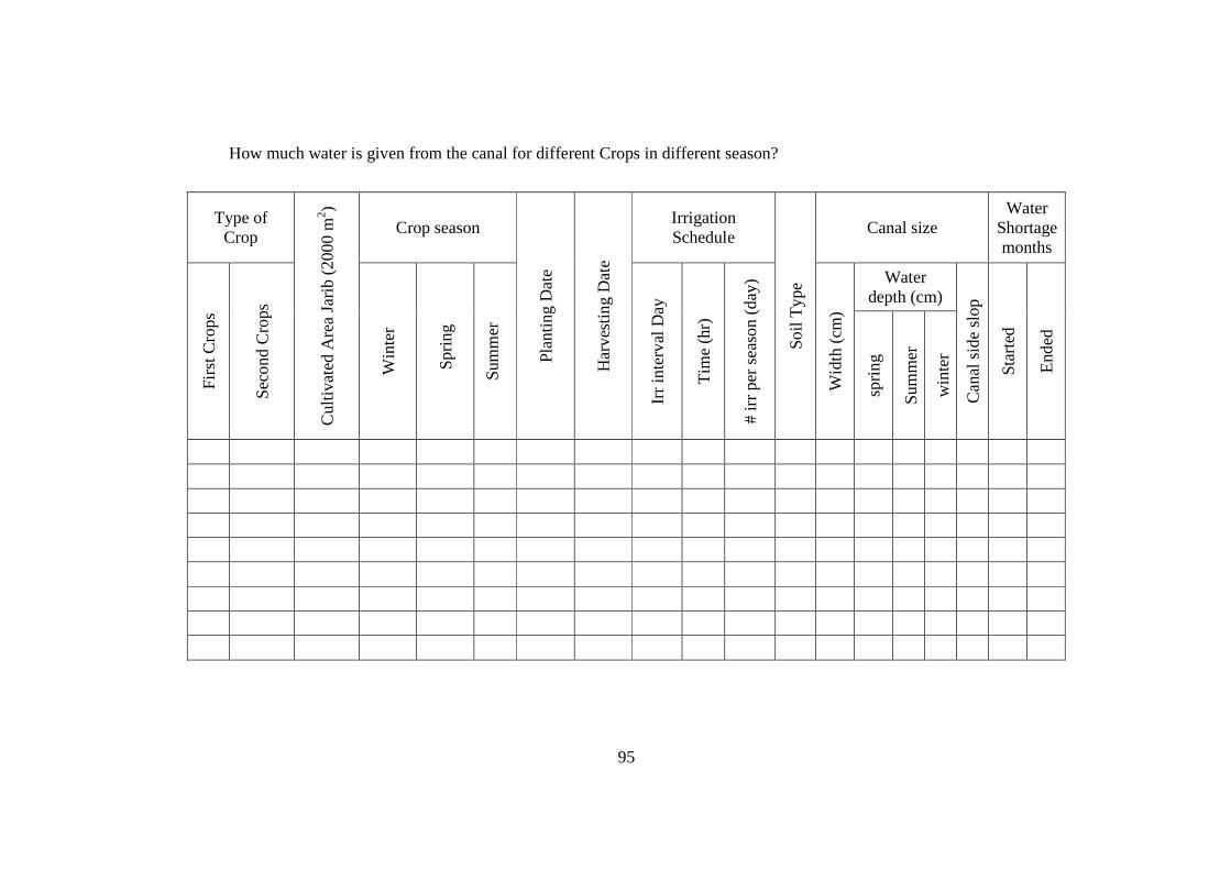
95

How much water is given from the canal for different Crops in different season?

Type of Crop

Cul

tivat

ed A

rea

Jarib

(2

00

0 m2 )

Crop season

Pla

ntin

g D

ate

Har

vest

ing

Dat

e

Irrigation Schedule

So

il T

ype

Canal size Water

Shortage months

Fir

st C

rop

s

Sec

on

d C

rops

Win

ter

S

prin

g

Sum

mer

Irr

inte

rval

Day

Tim

e (h

r)

# ir

r p

er s

eas

on

(d

ay)

Wid

th (

cm)

Water depth (cm)

Can

al s

ide

slo

p

Sta

rted

End

ed

sprin

g

Sum

mer

win

ter

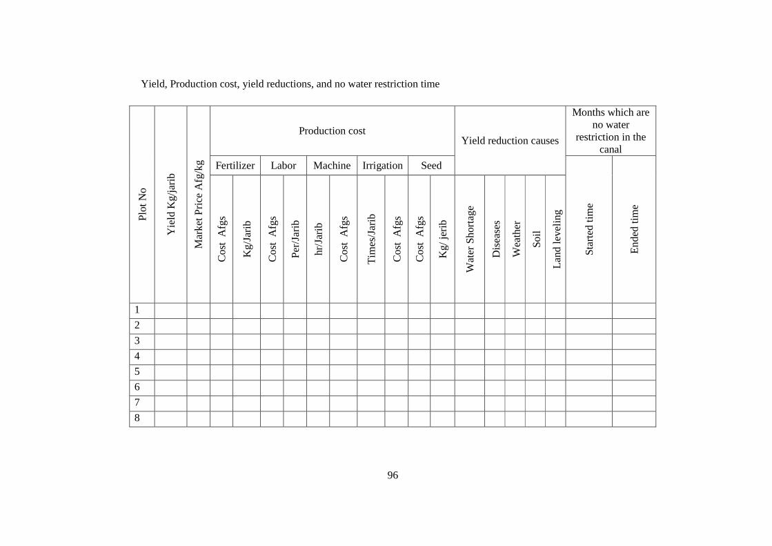
96

Yield, Production cost, yield reductions, and no water restriction time

Plo

t N

o

Yie

ld K

g/ja

rib

Mar

ket P

rice

Afg

/kg

Production cost Yield reduction causes

Months which are no water

restriction in the canal

Fertilizer Labor Machine Irrigation Seed

Sta

rted

tim

e

En

ded

tim

e

Co

st

Afg

s

Kg

/Jar

ib

Co

st

Afg

s

Per

/Ja

rib

hr/J

arib

Co

st

Afg

s

Tim

es/J

arib

Co

st

Afg

s

Co

st

Afg

s

Kg

/ je

rib

Wat

er S

hor

tag

e

Dis

ease

s

Wea

ther

So

il

Lan

d le

velin

g

1

2

3

4

5

6

7

8

97

6. Return Period of each crop

7. Is the available amount of water is enough for your crops?

8. Is current Scheduling is suitable for your Irrigation?

9. What are the alternative crops that you can cultivate during water shortage period?

10. Which crops are more profitable? ..............................................................................

(Thanks for your Kind Information)

Yes No

Yes No