options and investment strategies

Options and Investment Strategies Bernard Morard Ahmed Naciri

INTRODUCTION

he general framework suggested by Hakanson (1978), Cox (1976), and Ross T (1976) indicates that the appearance of an option market has the effect of increasing the general efficiency of financial markets by increasing the number of investment opportunities available to investors. One interesting aspect of the options market is the insurance component discussed by Leland (1980), Bookstaber and Clark (1983) and Tremolieres and Morard (1984). Aside from the characteristics inherent to options, option management in a portfolio context has been examined by many authors. Sears and Trennepohl(l982) have studied the risk to investors of portfolios composed exclusively of options. They conclude that option portfolios are more volatile than security portfolios but that a portfolio containing 20 securities allows for the elimination of 95% of the diversifiable risk. Booth, Tehranian, and Trennepohl (1985) have studied a variety of options strategies, including the buying of calls, the combined purchase of calls and risk-free assets, the buying of shares, and a fully-hedged strategy of writing calls on shares. Merton, Scholes, and Gladstein (1978, 1983) have examined fully-hedged writing option strategies. They find that different hedged strategies are qualitatively identical. Their results also show that any decrease in risk is obtained at the cost of a similar reduction in returns.

Generally, these studies seem to indicate that an investor cannot gain a particu- lar advantage by including options in his portfolio. However, this finding should be analyzed in light of the information contained in studies which indicate that 85% of written call options are used for hedging purposes. There is, of course, a difference between the interest in options as an investment instrument and their degree of popularity. Without analyzing the origin of this difference, one can make some remarks on methodological considerations such as the level of calculated returns, the various ways of constituting portfolios, and the level of hedging.

Generally, returns are computed semi-annually. This could be of no consequence even though the retention period seems long when not considering rigid strategies where the buyer of an option cannot exercise that option before its maturity. As for the constitution of portfolios, it is assumed that the investments in each asset are equally weighted. Markowitz’s (1959) solution is not optimal unless the number of securities is very large. Otherwise, as indicated by Sears and Trennepohl(1982), it is a “naive investment policy.” Finally, as far as the coverage of securities by writing

B. Morard is Professor, Universitk de Genbve.

A . Naciri is Professor, Universitk du Q d b e c h Montr6al.

The Journal of Futures Markets, Vol. 10, No. 5, 505-517 (1990) 0 1990 by John Wiley & Sons, Inc. ccc 0270-7314/901050505-13$04.00

options is concerned, various studies have suggested a simple approach that covers calls. Such strategies are always very questionable. This article attempts to avoid these methodological weaknesses.

In the general informational sense, the definition of an option strategy used here is based on the writings of Chiras and Manaster (1978), Manaster and Rendleman (1982), and Bhattacharya (1987). In equilibrium, the price of an option and its un- derlyng stock should reflect common information. The speed at which stock and option prices adjust to new information depends on the degree of friction in each market and the inherent riskheturn characteristics of the two securities. Option characteristics that are likely to appeal to “informed traders” include obtaining leverage positions in stock indirectly through options, smaller dollar outlays, and an upper bound at the top (in the case of long-position options). In these circum- stances: option market friction is lower, due to smaller dollar transaction costs, than those required for equivalent stock positions, margin conditions are less stringent, and the uptick rule for shortenant is suspended. Based on the advantages offered by option positions, one can conclude that the operation of the two markets can gen- erate some excess return when the portfolio is long on stock and short on call options. This article attempts to develop an original point of view on this subject.

This article takes a more realistic stand than previous studies, by introducing a new investment strategy which combines diversification and hedging, i.e., allowing a New York Stock Exchange investor not only to write calls on the Chicago Board of Options Exhange but offering him an original formula of calculating his or her optional hedging rates (optimal mix of stocks and options). This article eliminates several constraining hypotheses made by previous studies. Returns are calculated on daily basis, portfolios are composed of securities which do not have equal weight, and transactions are not free from costs. Several additional precautions were taken to solidify the findings. The analysis is conducted both ex-ante and ex-post and the test is carried out under both meadvariance and stochastic dominance criteria. The section which follows presents a new formulation of the ques- tion of hedged investments, both in terms of mean variance and stochastic dominance. Section I11 is devoted to an explanation of the sample and the methodology. Section IV contains the empirical research and presents the new efficient set which includes options and which is derived by using the stochastic dominance methodology. Concluding remarks appear in the final section.

11. INVESTMENT MODEL Markowitz’s (1959) diversification principle led to a number of different formula- tions of the investment model. The linear model developed by Garman (1977) and the model proposed by Danthine and Anderson (1981) are among the more recent. These models are oriented more towards an optimal hedged strategy than towards a global hedging strategy which combines diversification and hedging. However, the results published in Morard and TrBmolikres (1987) and Tr6molihre.s and Morard (1984) indicate that a global approach to hedged investments would be of interest.

The generalization of the meanhariance approach to hedging strategy can be explained in the following way. Consider a set of n financial assets simultaneously sold on two different markets: the spot market, where securities are transferred with certainty to the buyer; and the conditional market, where securities might never be transferred to the buyer. In this last case, the right to fail to execute the contract is immediately paid to the writer as a premium.

506 / MORARD AND NACIRI

Suppose that all the investments have the same maturity. If the conditional buyer does not execute the contract, the securities are sold by the writer on the spot market. Let call:

n . z((rifhi + cCui) = r

Z ( h i + U i ) = 1

i=l

n

i=l

0 5 hi I 1

0 I ui 5 1

i = 1, ... n

i = 1, ... n . -

x i = the $1 portion of capital invested in the i security, n = the number of assets considered on the spot market i = 1.. . , n

pi = the portion of xi covered by a conditional writer; if pi = 0, the security is not subject to any conditional contract writing; if p i = 1, the security is sold conditionally, and if 0 < pl < 1, for ki securities bought, pik i are sold conditionally.

rif = the return on the spot market for asset i; ric = the hedged return for asset i on the conditional market, for an in-

vestor who buys at t on the spot market and, at the same time, sells a call option or is asked to deliver the stock at (t + E ) , or for a seller on the spot market at e( t ) (maturity date).

Kf, ulf, ri,, uic the mean and standard deviation (respectively) of returns on the spot and the conditional markets.

The portfolio return could be expressed as: n

r(x, F ) = 2 ri(pi)xi i = l

with

ri(pi) = rif(1 - p i ) + ricpi

As established by Trgmoli6res and Morard (1984) make the following changes:

h, = xi(1 - pi), ~i = xipi (2)

ulf,,c the covariance between unhedged share i and a fully-hedged stock (all other alternatives being possible.)

We can then write:

(3)

A formulation close to that of the traditional meadvariance model is obtained but it includes twice as many variables. Also, the model defined in (3) is a generalization of the Markowitz model, provided it is obtainable by simply setting p i to 0.

OPTIONS AND INVESTMENT STRATEGIES / 507

The crucial point is to know whether an investor will gain an advantage by combining hedging and diversification, as suggested in (3). A common belief is that doubling the number of assets in a portfolio automatically leads to risk reduction. This belief needs to be clarified. On the one hand, diversification of over 20 securities will converge asymptotically with an irreducible minimal risk; on the other hand, it is very important to know the characteristics of the new securities included in the portfolio. For these reasons, it is not evident a priori that the model defined in (3) will lead to the creation of a “supra efficient set” which will dominate the efficient set characterized by simple diversification. It is therefore important to un- derstand that the results obtained here are not obvious, and must be tested. Two procedures are used to test this model. The first is the classical meadvariance analysis; the second is the stochastic dominance analysis.

First, the model in (3) can be classified as a meadvariance model with a special purpose. It allows an optimal solution for combined strategies and uses a distribution of two first moments only. However, if the underlying distributions are incom- pletely described by their mean and variance, an inconsistency might result (Ali, 1975). To avoid this, the stochastic dominance criteria is used concurrently. This provides a more efficient test no matter what form the distribution might take. Fur- thermore, even if the distributions are normal, the two analyses give the same results. The use of the stochastic dominance analysis is mainly intended to increase the validity of the findings.

Different algorithms have been used to test stochastic dominance: those in Porter, Ward, and Fergusson (1973); Levy and Kroll (1978); Bawa, Lindenberg, and Rafski (1979); Bawa, Bodurtha, Rao and Suri (1985), among others. This study is limited to discrete procedures using discontinuous distributions and assuming that the weight of the vector of the optimal portfolio is known. Although the algorithm defined in Bawa, Lindenberg, and Rafsky (1979) seems more suitable for large scale tests, the procedure described in Porter, Ward and Fergusson (1973) is used because this approach is sufficiently appropriate, precise, and easy to use for any reduced initial set of securities. This approach assumes that the two portfolios return vec- torsf and g are known through a total of N observahns and k observations per vector, then:

N = 2k

For a given realizationj, it is known that

f(r,) = l/k

The cumulative distribution F(r,) is obtained by the addition of the probabilities, no matter what the value of rl, j 4 n. For dominance to occur, one must have:

----> at the lst level, F(r,) 5 G(r,) for all n 5 N with a strict inequality for at least one n c: N where:

Fl(r , ) = $f(r,) , n = 2, 3 ,... N (4) J ” 1

--> at the 2”d level, Fz(rn) 5 Gl(rn) for all n 5 N, with a strict inequality €or at least one n 5 N, where:

F2(rn) = ~ ~ ( r ~ - , ) ( r ~ - r,-l) n = 2, 3 , . . . N n

1 = 2


--> at Yd level, Fz(r,) < G2(r,) for all n I 4 with a strict inequality for at least one n I N and Fz(r,,) 5 Gz(rn) , where:

111. SAMPLING AND METHODOLOGY To show the advantage of combined strategies, both ex-ante and ex-post analyses are used and a sample of 22 securities subject to simultaneous transactions at the New York Stock Exchange and at the Chicago Board of Options Exchange are cre- ated. Daily stock prices are taken from the Center of Research on Stock Prices file of the University of Chicago, and option prices from The Wall Street Journal. All the data are adjusted to include dividends and .6% transaction costs as suggested by Rubinstein and Cox (1985). The options selected are either at parity or out of the money, because those in the money are exercised. Options for ther terms of January, April, July, and October are chosen, because returns are calculated for specific time intervals: the period beginning January 1981 and ending October 1985 for the ex-ante analysis; and beginning January 1986 and ending December 1986 for the ex-post analysis. These periods cover different economic environments of increases and decreases in profitability. It is assumed that the maximum detention period does not exceed 15 days (Le., from the first day of the month to the option maturity date). The short interval choice can be justified in at least three ways. First, if longer initial intervals of retention are chosen one would have the choice of options for other terms, December, March, June, and September. Second, since the markets are dynamic, one can assume that buyers have rapid reactions; or, at least, that they can liquidate securities before their term (allowed by Ameri- can options). However, the interval can be shorter if securities are exercised by the buyer (or the contract is executed by him). Third, transactions on options are less steady for detention periods exceeding 15 days and this would lend to discontinuous data. The returns of unhedged and hedged positions are calculated for the same time intervals using the formulas below. Call:

~ ~ + ~ , p , ; wI ; option premium at time t, p e ; exercise price at time t, and d ; eventual dividend.

security price at time t + 1 and t,

Unhedged Position Return

rr+1 = [ P f + l - Pf + dl/Pt (7)

Hedged Position Return Hedged returns can be expressed in two different ways, depending upon whether the realized price is greater or lesser than the exercise price plus the premium. Note that the classical formulation “the realized price is greater or lesser than the exercise price” does not modify short returns but overestimates the hedged returns.


This situation can be formulated in the following two ways:

if p,+i pe + W: rt+i = [pe - pr + w]/pt, or (8)

ifp,+l I P e + W: (9) rf+l = [pt+l - p t + w + dl /p t ,

(9) automatically includes dividend for the writer of the option, if he has kept his security until maturity.

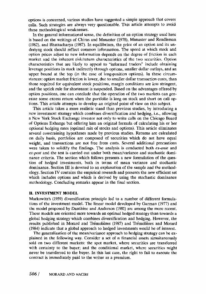
For every security 20 returns are obtained. Table I gives the mean and variance of returns taking into account transaction costs for each security, both at the level of the spot market and the conditional market. It can be noted that the hedged position does not systematically lead to a lower level of return for a lower level of risk, as suggested by Tinic and West (1979) (p. 142). As a matter of fact, one can see that in most cases levels of risk are significantly reduced in the case of hedged strategies. This situation can be explained theoretically by analyzing the problem in terms of distributions. If the existence of an “a priori” return distribution for a given security is assumed, the acquisition of a premium by the writer of a call option induces a translation and the exercise of this option up to the exercise price causes a truncation (Bookstaber, 1983). The initial distribution is reduced, thus reducing the risk as well in most cases.

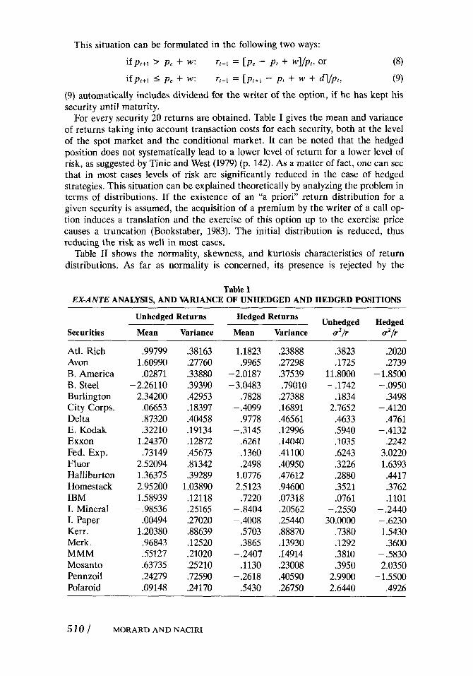
Table I1 shows the normality, skewness, and kurtosis characteristics of return distributions. As far as normality is concerned, its presence is rejected by the

Table I EX-ANTE ANALYSIS, AND VARIANCE OF UNHEDGED AND HEDGED POSITIONS

Unhedged Returns Hedged Returns Unhedged Hedged Securities Mean Variance Mean Variance a2/r a2/r

Atl. Rich Avon B. America B. Steel Burlington City Corps. Delta E. Kodak Exxon Fed. Exp. Fluor Halli burton Homestack IBM I. Mineral I. Paper Kerr. Merk . MMM Mosanto Pennzoil Polaroid

.99799 1.60990 .02871

2.34200 .06653 37320 .32210

1.24370 .73149

2.52094 1.36375 2.95 200 1.58939

.00494 1.20380 .96843 .55127 .63735 .24279 .09148

-2.26110

- .98536

.38163

.27760

.33880

.39390

.42953

.18397

.40458

.19134

.12872

.45673 31342 .39289

1.03890 .12118 .25165 .27020 A8639 .12520 .21020 .25210 .72590 .24170

1.1823 .9965

-2.0187 - 3.0483

.7828

.9778 - .3145

.6261

.1360

.2498 1.0776 2.5123 ,7220

- .4099

- 3404 - .4008

S703 .3865

.1130 -.2618

S430

- .2407

.23888

.27298

.37539 .79010

.27388

.16891

.46561

.12996

.14040

.41100

.40950

.47612

.94600

.07318

.20562

.25440 38870 .13930 .14914 .23008 .40590 ,26750

.3823

.1725 11 3000 - .1742

.1834 2.7652 .4633 S940 .lo35 .6243 .3226 .2880 .3521 .0761

30.0000 .7380 .1292 .3810 .3950

2.9900 2.6440

- .2550

.2020

.2739 - 1.8500 - .0950

.3498

.4761

.2242 3.0220 1.6393 .4417 .3762 .1101

- .2440 - .6230

- .4120

- .4132

1 S430 .3600

2.0350

.4926

- .5830

- 1.5500


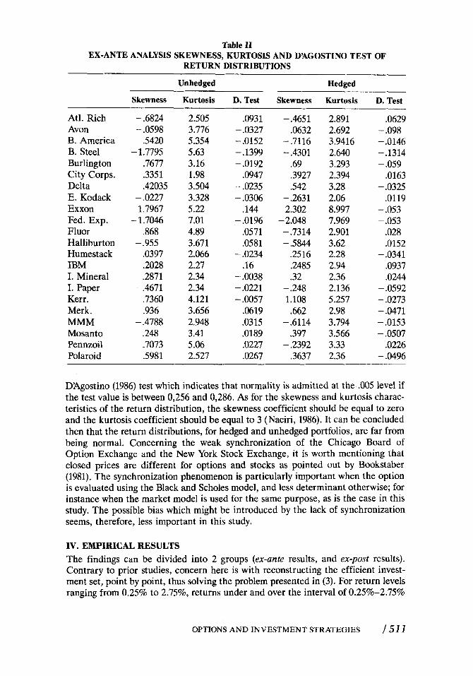
Table 11

RETURN DISTRIBUTIONS EX-ANTE ANALYSIS SKEWNESS, KURTOSIS AND D’AGOSTINO TEST OF

Un hedged Hedged

Skewness Kurtosis D. Test Skewness Kurtosis D. Test

Atl. Rich Avon B. America B. Steel Burlington City Corps. Delta E. Kodack Exxon Fed. Exp. Fluor Halliburton Humestack IBM I. Mineral I. Paper Kerr. Merk . MMM Mosanto Pennzoii Polaroid

- .6824 - .0598

S420

.7677

.3351

.42035

- 1.7795

- .0227 1.7967

- 1.7046 .868

- .955 .0397 .2028 .2871

.7360

.936

.248 -7073 S981

- .4671

- .4788

2.505 3.776 5.354 5.63 3.16 1.98 3.504 3.328 5.22 7.01 4.89 3.671 2.066 2.27 2.34 2.34 4.121 3.656 2.948 3.41 5.06 2.527

.0931 - .0327 - .0152 - .1399 -.0192

.0947 - .0235 - .0306

.144 - .0196

.0571

.0581 - .0234

.16 - .OO38 - .0221 - .OO57

.0619

.0315

.OM9

.0227

.0267

-.4651 .0632

-.7116 - .4301

.69

.3927

.542

2.302

-.7314 - 3 4 4

.2516 ,2485 .32

1.108 .662

- .6114 .397

- .2392 .3637

- .2631

- 2.048

- .248

2.891 2.692 3.9416 2.640 3.293 2.394 3.28 2.06 8.997 7.969 2.901 3.62 2.28 2.94 2.36 2.136 5.257 2.98 3.794 3.566 3.33 2.36

.0629 - .098 -.0146 -.1314 - .059

.0163

.0119 - .0325

- .053 - -053

.028

.0152

.0937

.0244

- .0341

- .0592 - .0273 - .0471 - .0153 - ,0507

.0226 - .0496

DAgostino (1986) test which indicates that normality is admitted at the .005 level if the test value is between 0,256 and 0,286. As for the skewness and kurtosis characteristics of the return distribution, the skewness coefficient should be equal to zero and the kurtosis coefficient should be equal to 3 (Naciri, 1986). It can be concluded then that the return distributions, for hedged and unhedged portfolios, are far from being normal. Concerning the weak synchronization of the Chicago Board of Option Exchange and the New York Stock Exchange, it is worth mentioning that closed prices are different for options and stocks as pointed out by Bookstaber (1981). The synchronization phenomenon is particularly important when the option is evaluated using the Black and Scholes model, and less determinant otherwise; for instance when the market model is used for the same purpose, as is the case in this study. The possible bias which might be introduced by the lack of synchronization seems, therefore, less important in this study.

IV. EMPIRICAL RESULTS The findings can be divided into 2 groups (ex-ante results, and ex-post results). Contrary to prior studies, concern here is with reconstructing the efficient investment set, point by point, thus solving the problem presented in (3). For return levels ranging from 0.25% to 2.75%, returns under and over the interval of 0.25%-2.75%


are omitted because they are not part of the efficient set. Different quadratic optimization algorithms may be used to solve this problem: the reduced gradient suggested by Wolfe (1983) and defined in Bazaraa and Shetty (1979) or the complementary algorithm proposed by Lemke (1970), to name only two. Wolfe’s procedure is used.

In Table I11 and Figure 1, the results of portfolio optimization are presented. These results seem to indicate that it is impossible to create a risk-free portfolio and that the efficient set of the hedged portfolio is the one which dominates Markowitz’s efficient set at every level of the return under 2.25% and that over a 2.25% return, Markowitz’s efficient set and the hedged portfolio efficient set are equivalent. It seems that the higher the desired return, the riskier the hedged portfolio is because the investor has to include in his hedged portfolio more options which are more risky.

This situation is confirmed by the stochastic dominance which compares the en- tire return distribution for each methodology, hedged and unhedged portfolio, and which leads to the conclusion that the returns from the hedged portfolio exceed those of the unhedged portfolios for all 20 observations. Note, however, that the meadvariance criteria always give the same ranking as stochastic dominance.

Table IV shows the results obtained, using hedged and unhedged equally weighted portfolios.

The results presented in Table IV confirm the common belief that hedged strategies allow investors to decrease their risk, but lead to decreased returns. Also, the equally weighted portfolio does not belong to the efficient set any more than the equally weighted hedged portfolio belongs to the supra efficient set. This, perhaps, is why previous studies using equally weighted portfolios have failed to demonstrate the dominance of hedged strategies over unhedged strategies, and to show the advantage of hedged strategies for the investor. At this point, the optimal hedge ratio is calculated.

Table 111

STRATEGIES AND STOCHASTIC DOMINANCE TEST EX-ANTE ANALYSIS: RISK AND RETURN OF UNHEDGED AND HEDGED

Stochastic Un hedged Hedged Dominance

Portfolio Portfolio Strategy Risk Strategy Risk Test Number Return (1) (2) (2) > (1)

1 2 3 4 5 6 7 8 9

10 11

.25% S O % .75%

1.00% 1.25% 1 SO% 1.75% 2.00% 2.25% 2.50% 2.75%

.2142941 ,2023502 .2203 100 .2089113 ,3184350 .4441050 .7288830

1.2488000 2.1225100 3.4980000 5.9960000

.OW410

.088130

.lo3573

.140559

.227435

.402172

.682792 1.225870 2.115700 3.501520 6.001200

1st order 1st order 1st order 1st order 1st order 1st order 3rd order 1st order

no dominance no dominance no dominance


r risk

Figure 1 Efficient Sets .

To calculate the hedge ratio, eq. (3) and set pi are used as follows:

ui ui + hi Pi = ~

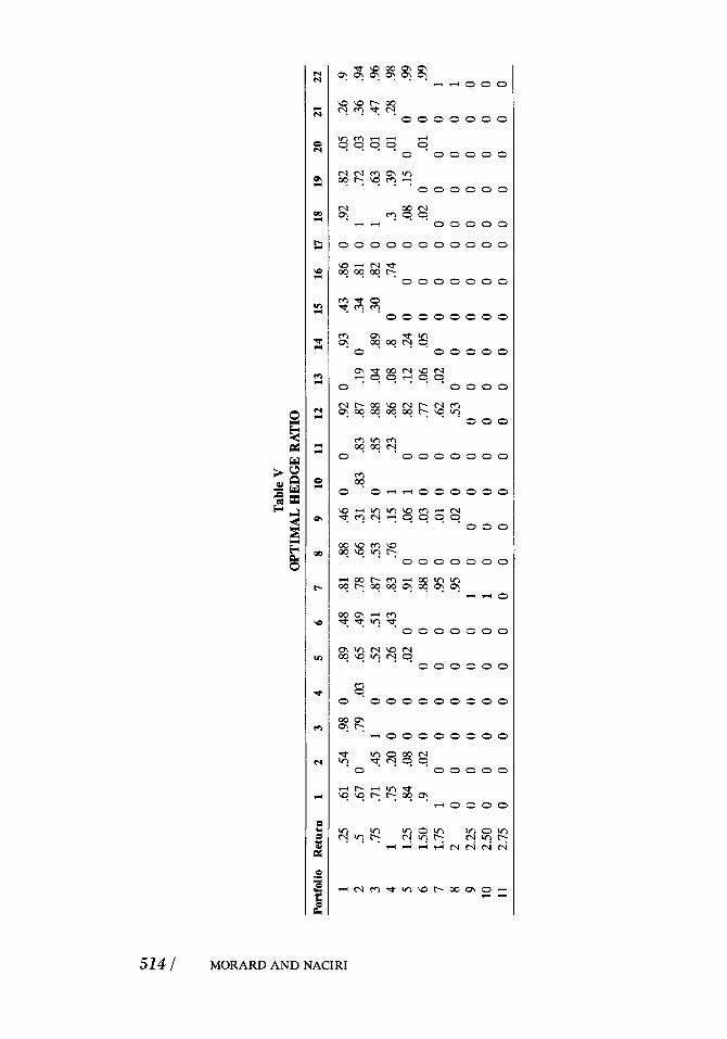
The optimal hedging for the security i is then obtained. Table V indicates that the concept of a global hedging portfolio suggested by Howard and DAntonio (1984) does not apply here. The reason for this is that true portfolios are used for more than one security. Furthermore, the optimal hedge ratio is dynamic and varies with each portfolio. Also, full hedging of a portfolio, i.e., loo%, is a special case in this analysis. For high levels of returns, i.e., for 1.75% and over, the optimal hedge approaches zero. The reason is that, at these levels, more options are required for hedging purposes and these options are more risky.

An ex-post analysis is conducted to improve the robustness of the findings. Table VI presents the results of the portfolio optimization suggested in this article. The optimal hedged ratios calculated in the previous section are applied to the New York Stock Exchange and the Chicago Board of Options Exchange regarding stocks and options respectively for the period beginning January 1986 and ending Decem- ber 1986. It seems that in 1986 a New York Stock Exchange investor using the Chicago Board of Options Exchange at the same time would have been better off

Table IV RISK AND RETURN OF EQUALLY WEIGHTED PORTFOLIOS, UNHEDGED AND

FULLY HEDGED STRATEGIES

Return Risk (r) (a2) u2/r

~~ ~~

Equally weighted portfolio unhedged strategy .77708 .6301 .81 Equally weighted portfolio hedged strategy ,4638 .4729 1.0796


U

Tabl

e V

O

PTIM

AL

HE

DG

E R

ATI

O

Port

folio

R

etur

n 1

2 3

4 5

6 7

8 9

10

11

12

13

14

15

16

17

18

19

20

21

22

1 .25

.6

1 .5

4 .9

8 0

.89

.48

.81

.88

.46

0 0

.92

0 .9

3 .4

3 .8

6 0

.92

.82

.05

.26

.9

2 .5

.67

0 .79

.0

3 .6

5 .4

9 .7

8 .66

.31

.83

.83

.87

.19

0 .3

4 .8

1 0

1 .7

2 .0

3 .3

6 .9

4 3

.75

.71

.45

1 0

.52

.51

.87

.53

.25

0 .85

.88

.04

.89

.30

.82

0 1

.63

.01

.47

.96

4 1

.75

.20

0 0

.26

.43

.83

.76

.15

1 .2

3 .86

.0

8 .8

0

.74

0 .3

.3

9 .0

1 .2

8 .9

8 5

1.25

.8

4 .0

8 0

0 .0

2 0

.91

0 .0

6 1

0 .8

2 .1

2 .2

4 0

0 0

.08

.15

0 0

.99

6 1.

50

.9

.02

0 0

0 0

.88

0 .0

3 0

0 .7

7 .0

6 .0

5 0

0 0

.02

0 .0

1 0

.99

7 1.

75

1 0

0 0

0 0

.95

0 .0

1 0

0 .6

2 .0

2 0

0 0

0 0

0 0

0 1

8 2

00

00

00

.95

0

.02

0

0 .5

30

0

0 0

00

0

0 0

1 9

2.2

50

0

0 0

0 0

10

0 0

0 0

0 0

0 0

00

0

0 0

0 10

2

.50

0

0 0

0 0

0 1

0 0

0 0

0 0

0 0

0 0

0

0 0

0 0

11

2.7

50

0

0 0

0 0

0 0

0 0

0 0

0 0

0 0

00

0

0 0

0

Table VI

STRATEGIES AND STOCHASTIC DOMINANCE TEST EX-POST ANALYSIS, RISKS AND RETURNS OF UNHEDGED AND HEDGE

Stochastic Portfolio Dominance Number r a2 r d Test (2) > (1)

Unhedged Portfolio (1) Hedged Portfolio (2)

1 -1.1718 3.239 -2.513 3.364 no dominance 2 - 1.454 3.1692 -2.039 2.8976 1st order 3 - 1.065 2.7197 -1.511 2.5686 1st order 4 - 1.356 1 A266 - .9292 2.1876 1st order 5 - .414 1.8378 - A627 1.9602 1st order 6 - .7398 1.8136 - .968 1.804 no dominance 7 - 1.35857 2.241 - 1.4164 2.1643 no dominance 8 - 1.4741 2.3506 - 1.2706 2.2963 1st order 9 - S463 2.1679 .532 2.1815 1st order

10 -2.3163 4.068 .6332 2.346 no dominance 11 -3.511 4.1745 1.767 3.7117 1st order

than an investor using the New York Stock Exchange only. This is concluded from the returns and risks on hedged and unhedged portfolios and confirmed by the stochastic dominance test.

The ex-ante and ex-post analyses seem to confirm the superiority of the investment strategy suggested in this article over the classical meadvariance strategy and over other known hedged strategies.

V. CONCLUDING REMARKS This article suggests an investment model oriented towards global hedging that combines diversification and hedging. The superiority of such global hedging over Markowitz’s strategy is suggested and an original approach to calculating the optimal hedge ratio is proposed. In this regard, two different analyses are used: ex-ante and ex-post analysis, along with two different tests: meadvariance and stochastic dominance.

The main empirical findings are as follows: (1) The analysis indicates that an investor can earn excess returns in covered call writing instead of holding a Markowithz’s portfolio and (2) it is possible to calculate the optima1 hedge ratio. This ratio, although different for each portfolio, never equals full hedging; i.e., equals one as suggested by previous studies.

Several considerations appear relevant from this analysis: (1) The capacity of the suggested model to capture the effect of hedging adds usefulness to classical diversification strategies followed by hedging and might prove to be useful in financial decision making. It seems clear that it is advantageous for a New York Stock Ex- change investor to be able to write options on the Chicago Board of Options Ex- change, If he is not allowed to do so, he is kept from operating with optimal means; (2) the findings concerning excess returns of hedged strategy over classical diversification might be viewed as conservative. The same transaction costs are used for both stocks and options; however, in practice, costs for options are lower; (3) the solidity of the findings are improved by using ex-ante and ex-post analyses in mean/ variance and a stochastic dominance environments and by paying special attention


to other methodological considerations such as the use of daily returns and taking into account dividends and transaction costs; and (4) although, as suggested by Bookstaber (1981), synchronization is not important in the case of studies like this, the findings should be interpreted in light of the non-synchronization which charac- terizes daily transactions on the Chicago Board of Option Exchange and the New York Stock Exchange. It seems that the non-synchronization phenomena alone cannot explain the findings.

A general equilibrium hedging model which includes the writing of calls and all other term contracts needs to be researched and developed.

Bibliography Ali, M. M. (1975): “Stochastic Dominance and Portfolio Analysis,” Journal of Financial Eco-

Bazaraa, M. S., and Shetty, C. M. (1979): Non Linear Programming; Theory and Algorithms,

Bawa, V. S., Lindenberg, E. B., and Rafsky. (1979): ‘An Efficient Algorithm to Determine

Bawa, V.S., Bodurtha, J. R. J., Rao, M. R., and Suri, H. L. (1985): “On Determination of

Bhattacharya, M. (1987): “Price Change of Related Securities: The Case of Call Options and

Bookstaber, R. (1981): “Observed Option Mispricing and the Nonsimultaneity of Stock and

Bookstaber, R. (1983): Option Pricing and Strategies in Investing, Addison-Wesley. Bookstaber, R., and Clark, R. (1983): ‘An Algorithm to Calculate the Return of Portfolio

Booth, J. R., Tehranian, A., and Trennepohl, G. L. (1985): “Efficiency Analysis and Option

Chiras, D.P., and Manaster, S. (1978): “The Information Content of Option Prices and a

Cox, J. C. (1976): “Futures Trading and Market Information,” Journal of Political Economy,

DAgostino, R. B., and Stephens, M. A. (1986): Goodness-of-Fit Techniques-Statistics,

Danthine, J. P., and Anderson, R.W. (1981): “Cross Hedging,” Journal of Political Economy,

Garman, M. B. “An Algebra for Evaluating Hedge Portfolio,” Journal of Financial Econom-

Hakanson, N. (1978): “Welfare Aspects of Options and Supershares,” Journal of Finance, 33:

Howard, C.T., and DAntonio, L. J. (1984): ‘A risk-return Measure of Hedging Effective-

Leland, H. E. (1980): “Who Should Buy Portfolio Insurance?”, Journal of Finance, 2:581-594. Lemke, C. E. (1970): “Recent Results on Complementary Problem,” In Non Linear Program-

Levy, H., and Kroll, Y. (1978): “Ordering Uncertain Options with Borrowing and Lending,”

nomics, 2:205-229.

New York: John Wiley.

Stochastic Dominance Admissible Sets,” Management Science, 25:609-622.

Stochastic Dominance Optimal Sets,” Journal of Finance, 2:417-434.

Stocks,” Journal of Financial and Quantitative Analysis, 1:l-15.

Option Quotations,” Journal of Business, 1:141-153.

with Option Positions,” Management Science, 29:419-479.

Portfolio Selection,” Journal of Financial and Quantitative Analysis, 4:435-450.

Test of Market Efficiency,” Journal of Financial Economics, 6:213-234.

3:1215-1237.

Dekkers, Vol. 68.

62:1182-1196.

ics, 2:210-235.

759-776.

ness,” Journal of Financial and Quantitative Analysis, 19, 1:lOl-112.

ming, Rosen, J. B., Magasarian, 0. L., and Ritter, K. Eds.

Journal of Finance, 7:125-130.

51 6 / MORARD AND NACIRI

Manaster, S., and Rendleman, R. J. (1982): “Option Prices as Predictor of Equilibrium Stock

Markowitz, H. (1959): Portfolio Selection, New York: Wiley. Merton, R., Scholes, M., and Gladstein, M. (1978): “The Returns and Risk of Alternative

Call Option Portfolio Investment Strategies,” Journal of Business, 2:183-242. Merton, R., Scholes, M., and Gladstein, M. (1983): “The Returns and Risk of Alternative

Portfolio Investment Strategies,” Journal of Business, 2:l-55. Morard, B., and TrCmolisres, R. (1987): “Stratigies dominantes et fronti6res Supra Effi-

caces,” Actes du Congr& ASAC, Toronto, 18:194-199. Naciri, A. (1986, June): “Chypothsse de la distribution normale dans le cas d’kvknements

simultanCs,” Canadian Journal of Administrative Sciences, 99-113. Porter, R. B., Ward, J. R., and Ferguson, D. L. (1973): “Efficient Algorithms for Conducting

Stochastic Dominance Tests on Large Numbers of Portfolios,” Journal of Financial and Quantitative Analysis, 1:71-81.

Prices,” The Journal of Finance, 4:1043-1057.

Rubinstein, M., and Cox, J. C. (1985): Option Markets, Prentice-Hall. Ross, S. (1976): “Options and Efficiency,” Quarterly Journal of Economics, 90:75-89. Sears, R. S., and Trennepohl, G. L. (1982): “Measuring Portfolio Risk in Option,” Journal of

Financial and Quantitative Analysis, 3:392-409. Trennepohl, G., and Dukes, W. P. (1981): ‘An Empirical Test of Option writing and Buying

Strategies utilizing in-the-Money and out-the-Money Contracts,” Journal of Business Fi- nance and Accounting, 2:185-202.

Tinic, S. M., and West, R. R. (1979): Investing in Securities: An Efficient Markets Approach, Addison Wesley.

TrCmolEres, R., and Morard, B. (1984): “Couverture et Diversification: un mCme mod6le EVP d’EspCrance-Variance-Param&ri,” Presented at 5th “Journke Internationale de MFFZ’’, IEC Grenoble.

Wolfe, P. (1983): Methods of Nonlinear Programming, in Recent Advance in Mathematical Programming, Grove, R. L., and Wolfe, P. Eds.

OPTIONS AND INVESTMENT STRATEGIES / 51 7

options and investment strategies

Documents