optimizing the exponential sine sweep (ess) signal for in ...€¦ · ess signal: (a) with fade-in...

Optimizing the exponential sine sweep (ESS) signal for in situ measurements on noise barriers

Massimo Garai

Department of Industrial Engineering, University of Bologna, Bologna, Italy.

Paolo Guidorzi

Department of Industrial Engineering, University of Bologna, Bologna, Italy.

Summary

The measurement of sound reflection and airborne sound insulation of noise barriers in based on

the acquisition of impulse responses by means of digital devices. The most widely used methods

employ MLS (Maximum Length Sequence) or ESS (Exponential Sine Sweep) as test signals. The

theory behind MLS generation and use is well developed and does not involve computational

problems. That is why in CEN/TS 1793-5:2003 an MLS signal is recommended. During the

European project QUIESST also an ESS signal was applied. The ESS signal has some advantages

over MLS, such as a better signal to noise ratio (SNR) and a robust non-linearity rejection. Anyway,

the generation of an ESS signal and the subsequent analysis of impulse responses involve some

problems whose solutions are not yet common practice. These solutions are discussed here and

practical application examples are presented.

PACS no. 43.58.Gn, 43.58.Kr, 43.55.Mc, 43.60.Ac

1. Introduction

The use of a MLS (Maximum Length Sequence)

signal for measuring impulse responses is well

established [1], [2], [3]. The sine sweep signal is

also widely used [4]. In particular, the ESS

(Exponential Sine Sweep) signal has gained

considerable interest since Farina introduced it in

2000 [5] and refined it in 2007 [6]. It has some

advantages over MLS and some drawbacks. The

main advantage of the ESS method is the separation

of the linear part of the measured impulse response

of the system from most part of the harmonic

distortion, even if recent works have shown that

some amount of odd orders distortion still remains,

as formally proved in 2011 Torras et al. [7]. The

partial contamination of nonlinear distortion to the

causal part of the impulse response was earlier

found by Cirik in 2007 [8] and confirmed by other

authors such as Kemp et al. in 2011 [9] or Dietrich

et al. in 2013 [10] or Gusky et al. in 2014 [11]. The

separation of the most part of distortion from the

linear part permits to have a much better signal to

noise ratio (SNR) than with MLS, because the

impulse response is free from the spurious peaks

distributed on the time axis typically caused by

distortion when using MLS. Using ESS instead, the

impulse response is recovered by means of an

aperiodic linear convolution, avoiding the time-

aliasing problem of MLS. Moreover, employing an

ESS measurement signal allows to easily describe

the nonlinearities of the measured system by means

of the Volterra model [12] and its simplified

implementation (Diagonal Volterra model). The

crest factor of about 3 dB of the ESS can be

exploited performing high power measurements in

(steady) noisy conditions. Typically, in similar

conditions the ESS has a dynamic range of about 15

dB higher than MLS.

2. Effect of impulsive background noise

Whereas stationary background noise can be

somehow rejected and compensated in different

ways for both MLS and ESS methods [11],

impulsive noises can contaminate the data sampled

using an ESS signal, causing spurious effects on the

deconvolved impulse response in form of a

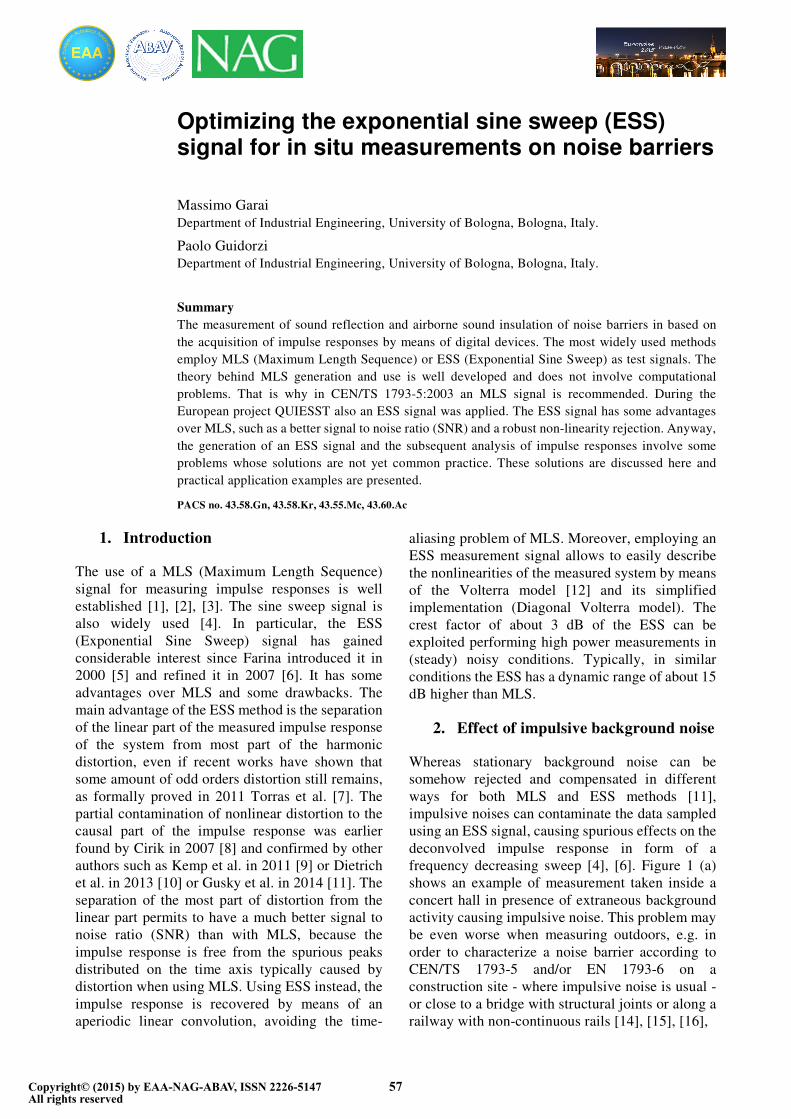
frequency decreasing sweep [4], [6]. Figure 1 (a)

shows an example of measurement taken inside a

concert hall in presence of extraneous background

activity causing impulsive noise. This problem may

be even worse when measuring outdoors, e.g. in

order to characterize a noise barrier according to

CEN/TS 1793-5 and/or EN 1793-6 on a

construction site - where impulsive noise is usual -

or close to a bridge with structural joints or along a

railway with non-continuous rails [14], [15], [16],

Copyright© (2015) by EAA-NAG-ABAV, ISSN 2226-5147All rights reserved

57

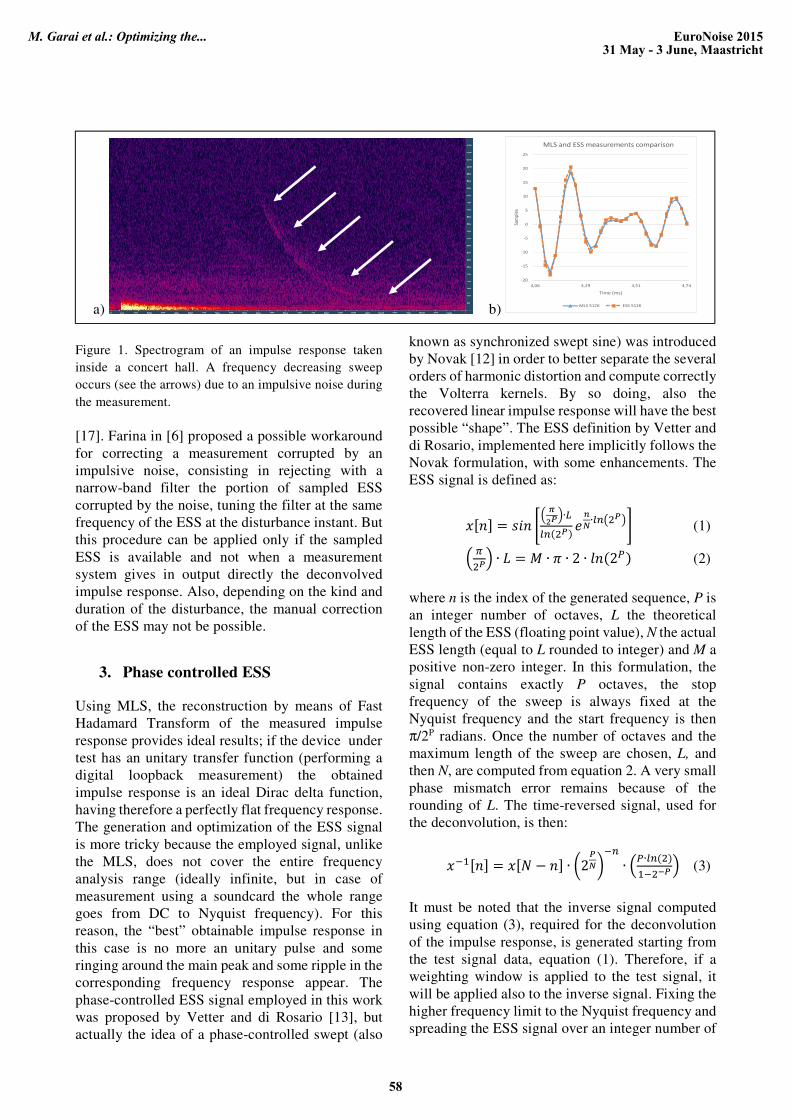
Figure 1. Spectrogram of an impulse response taken

inside a concert hall. A frequency decreasing sweep

occurs (see the arrows) due to an impulsive noise during

the measurement.

[17]. Farina in [6] proposed a possible workaround

for correcting a measurement corrupted by an

impulsive noise, consisting in rejecting with a

narrow-band filter the portion of sampled ESS

corrupted by the noise, tuning the filter at the same

frequency of the ESS at the disturbance instant. But

this procedure can be applied only if the sampled

ESS is available and not when a measurement

system gives in output directly the deconvolved

impulse response. Also, depending on the kind and

duration of the disturbance, the manual correction

of the ESS may not be possible.

3. Phase controlled ESS

Using MLS, the reconstruction by means of Fast

Hadamard Transform of the measured impulse

response provides ideal results; if the device under

test has an unitary transfer function (performing a

digital loopback measurement) the obtained

impulse response is an ideal Dirac delta function,

having therefore a perfectly flat frequency response.

The generation and optimization of the ESS signal

is more tricky because the employed signal, unlike

the MLS, does not cover the entire frequency

analysis range (ideally infinite, but in case of

measurement using a soundcard the whole range

goes from DC to Nyquist frequency). For this

reason, the “best” obtainable impulse response in

this case is no more an unitary pulse and some

ringing around the main peak and some ripple in the

corresponding frequency response appear. The

phase-controlled ESS signal employed in this work

was proposed by Vetter and di Rosario [13], but

actually the idea of a phase-controlled swept (also

known as synchronized swept sine) was introduced

by Novak [12] in order to better separate the several

orders of harmonic distortion and compute correctly

the Volterra kernels. By so doing, also the

recovered linear impulse response will have the best

possible “shape”. The ESS definition by Vetter and

di Rosario, implemented here implicitly follows the

Novak formulation, with some enhancements. The

ESS signal is defined as:

�� = �� ∙�

�� ∙�� (1)

�� ∙ � = � ∙ � ∙ 2 ∙ ��2!� (2)

where n is the index of the generated sequence, P is

an integer number of octaves, L the theoretical

length of the ESS (floating point value), N the actual

ESS length (equal to L rounded to integer) and M a

positive non-zero integer. In this formulation, the

signal contains exactly P octaves, the stop

frequency of the sweep is always fixed at the

Nyquist frequency and the start frequency is then

π/2P radians. Once the number of octaves and the

maximum length of the sweep are chosen, L, and

then N, are computed from equation 2. A very small

phase mismatch error remains because of the

rounding of L. The time-reversed signal, used for

the deconvolution, is then:

�"#�� = ��$ − �� ∙ &2��'"� ∙ !∙��

#"�(� (3)

It must be noted that the inverse signal computed

using equation (3), required for the deconvolution

of the impulse response, is generated starting from

the test signal data, equation (1). Therefore, if a

weighting window is applied to the test signal, it

will be applied also to the inverse signal. Fixing the

higher frequency limit to the Nyquist frequency and

spreading the ESS signal over an integer number of

a) b)

-20

-15

-10

-5

0

5

10

15

20

25

4,06 4,29 4,51 4,74

Sam

ple

s

Time (ms)

MLS and ESS measurements comparison

MLS 512K ESS 512K

EuroNoise 201531 May - 3 June, Maastricht

M. Garai et al.: Optimizing the...

58

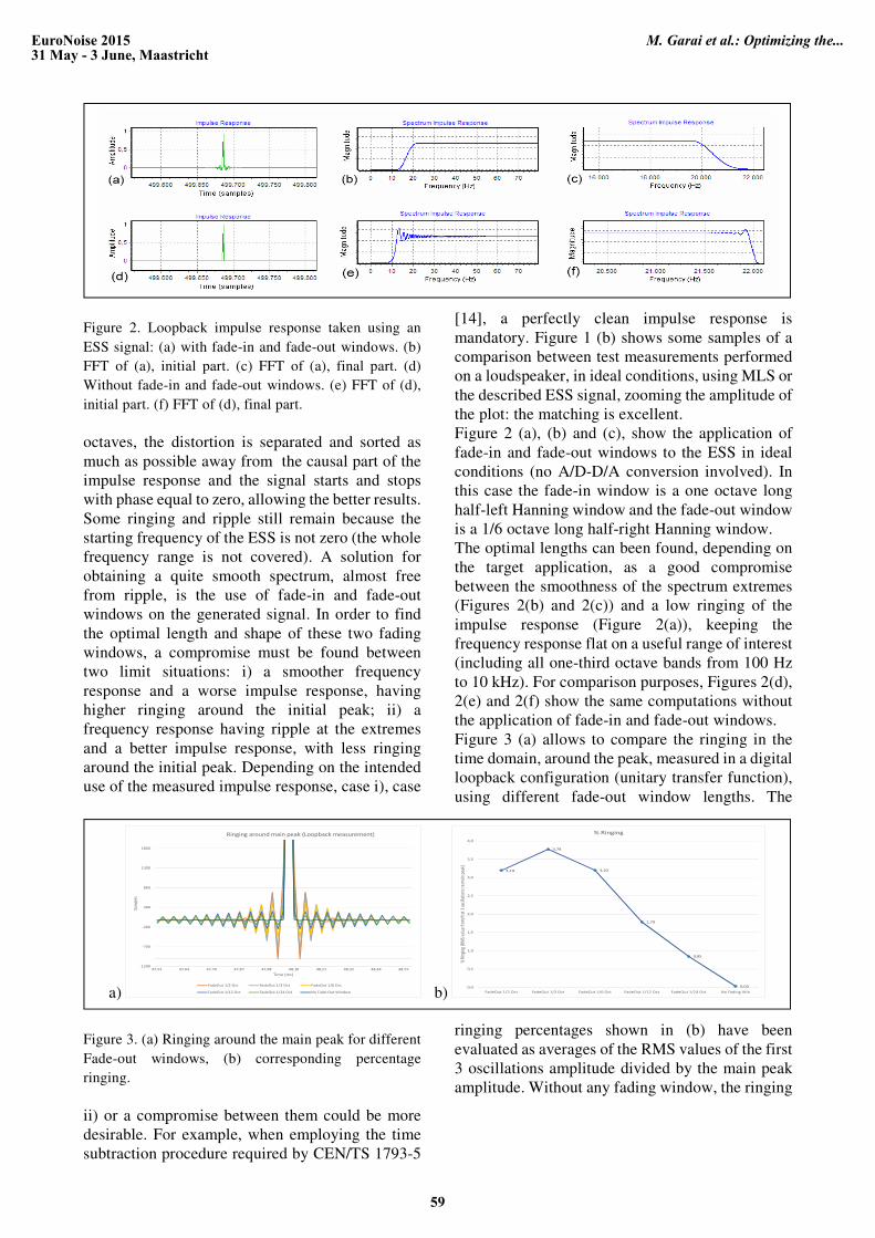
Figure 2. Loopback impulse response taken using an

ESS signal: (a) with fade-in and fade-out windows. (b)

FFT of (a), initial part. (c) FFT of (a), final part. (d)

Without fade-in and fade-out windows. (e) FFT of (d),

initial part. (f) FFT of (d), final part.

octaves, the distortion is separated and sorted as

much as possible away from the causal part of the

impulse response and the signal starts and stops

with phase equal to zero, allowing the better results.

Some ringing and ripple still remain because the

starting frequency of the ESS is not zero (the whole

frequency range is not covered). A solution for

obtaining a quite smooth spectrum, almost free

from ripple, is the use of fade-in and fade-out

windows on the generated signal. In order to find

the optimal length and shape of these two fading

windows, a compromise must be found between

two limit situations: i) a smoother frequency

response and a worse impulse response, having

higher ringing around the initial peak; ii) a

frequency response having ripple at the extremes

and a better impulse response, with less ringing

around the initial peak. Depending on the intended

use of the measured impulse response, case i), case

Figure 3. (a) Ringing around the main peak for different

Fade-out windows, (b) corresponding percentage

ringing.

ii) or a compromise between them could be more

desirable. For example, when employing the time

subtraction procedure required by CEN/TS 1793-5

[14], a perfectly clean impulse response is

mandatory. Figure 1 (b) shows some samples of a

comparison between test measurements performed

on a loudspeaker, in ideal conditions, using MLS or

the described ESS signal, zooming the amplitude of

the plot: the matching is excellent.

Figure 2 (a), (b) and (c), show the application of

fade-in and fade-out windows to the ESS in ideal

conditions (no A/D-D/A conversion involved). In

this case the fade-in window is a one octave long

half-left Hanning window and the fade-out window

is a 1/6 octave long half-right Hanning window.

The optimal lengths can been found, depending on

the target application, as a good compromise

between the smoothness of the spectrum extremes

(Figures 2(b) and 2(c)) and a low ringing of the

impulse response (Figure 2(a)), keeping the

frequency response flat on a useful range of interest

(including all one-third octave bands from 100 Hz

to 10 kHz). For comparison purposes, Figures 2(d),

2(e) and 2(f) show the same computations without

the application of fade-in and fade-out windows.

Figure 3 (a) allows to compare the ringing in the

time domain, around the peak, measured in a digital

loopback configuration (unitary transfer function),

using different fade-out window lengths. The

ringing percentages shown in (b) have been

evaluated as averages of the RMS values of the first

3 oscillations amplitude divided by the main peak

amplitude. Without any fading window, the ringing

a) b)

-1200

-700

-200

300

800

1300

1800

47,53 47,64 47,76 47,87 47,98 48,10 48,21 48,32 48,44 48,55

Sam

ples

Time (ms)

Ringing around main peak (Loopback measurement)

FadeOut 1/2 Oct FadeOut 1/3 Oct FadeOut 1/6 Oct

FadeOut 1/12 Oct FadeOut 1/24 Oct No Fade-Out Window

3,19

3,78

3,20

1,79

0,85

0,030,0

0,5

1,0

1,5

2,0

2,5

3,0

3,5

4,0

FadeOut 1/2 Oct FadeOut 1/3 Oct FadeOut 1/6 Oct FadeOut 1/12 Oct FadeOut 1/24 Oct No Fading Win

% R

ingi

ng (R

MS

valu

e fr

om fi

rst

3 os

cilla

tions

re

mai

n pe

ak)

% Ringing



59

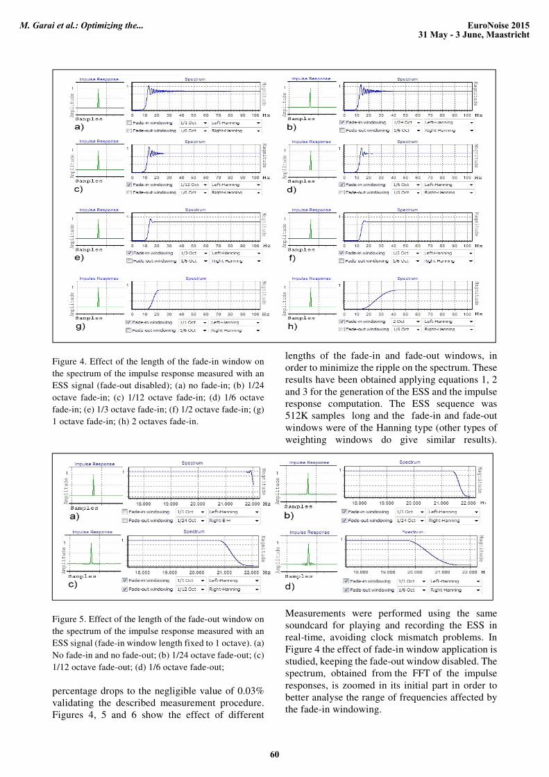
Figure 4. Effect of the length of the fade-in window on

the spectrum of the impulse response measured with an

ESS signal (fade-out disabled); (a) no fade-in; (b) 1/24

octave fade-in; (c) 1/12 octave fade-in; (d) 1/6 octave

fade-in; (e) 1/3 octave fade-in; (f) 1/2 octave fade-in; (g)

1 octave fade-in; (h) 2 octaves fade-in.

Figure 5. Effect of the length of the fade-out window on

the spectrum of the impulse response measured with an

ESS signal (fade-in window length fixed to 1 octave). (a)

No fade-in and no fade-out; (b) 1/24 octave fade-out; (c)

1/12 octave fade-out; (d) 1/6 octave fade-out;

percentage drops to the negligible value of 0.03%

validating the described measurement procedure.

Figures 4, 5 and 6 show the effect of different

lengths of the fade-in and fade-out windows, in

order to minimize the ripple on the spectrum. These

results have been obtained applying equations 1, 2

and 3 for the generation of the ESS and the impulse

response computation. The ESS sequence was

512K samples long and the fade-in and fade-out

windows were of the Hanning type (other types of

weighting windows do give similar results).

Measurements were performed using the same

soundcard for playing and recording the ESS in

real-time, avoiding clock mismatch problems. In

Figure 4 the effect of fade-in window application is

studied, keeping the fade-out window disabled. The

spectrum, obtained from the FFT of the impulse

responses, is zoomed in its initial part in order to

better analyse the range of frequencies affected by

the fade-in windowing.



60

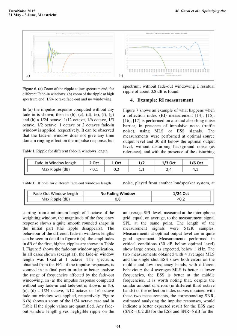
Figure 6. (a) Zoom of the ripple at low spectrum end, for

different Fade-in windows; (b) zoom of the ripple at high

spectrum end, 1/24 octave fade-out and no windowing.

In (a) the impulse response computed without any

fade-in is shown; then in (b), (c), (d), (e), (f), (g)

and (h) a 1/24 octave, 1/12 octave, 1/6 octave, 1/3

octave, 1/2 octave, 1 octave or 2 octaves fade-in

window is applied, respectively. It can be observed

that the fade-in window does not give any time

domain ringing effect on the impulse response, but

Table I. Ripple for different fade-in windows length.

Table II. Ripple for different fade-out windows length.

starting from a minimum length of 1 octave of the

weighting window, the magnitude of the frequency

response shows a quite smooth rounded shape in

the initial part (the ripple disappears). The

behaviour of the different fade-in windows lengths

can be seen in detail in figure 6 (a); the amplitudes

in dB of the first, higher, ripples are shown in Table

I. Figure 5 shows the fade-out window application.

In all cases shown (except a)), the fade-in window

length was fixed at 1 octave. The spectrum,

obtained from the FFT of the impulse responses, is

zoomed in its final part in order to better analyse

the range of frequencies affected by the fade-out

windowing. In (a) the impulse response computed

without any fade-in and fade-out is shown; in (b),

(c), (d) a 1/24 octave, 1/12 octave or 1/6 octave

fade-out window was applied, respectively. Figure

6 (b) shows a zoom of the 1/24 octave case and in

Table II the ripple values are quantified. Any fade-

out window length gives negligible ripple on the

spectrum; without fade-out windowing a residual

ripple of about 0.8 dB is found.

4. Example: RI measurement

Figure 7 shows an example of what happens when

a reflection index (RI) measurement [14], [15],

[16], [17] is performed on a sound absorbing noise

barrier, in presence of impulsive noise (traffic

noise), using MLS or ESS signals. The

measurements were performed at optimal source

output level and 30 dB below the optimal output

level, without disturbing background noise (as

reference), and with the presence of the disturbing

noise, played from another loudspeaker system, at

an average SPL level, measured at the microphone

grid, equal, on average, to the measurement signal

SPL at the same point. The length of the

measurement signals were 512K samples.

Measurements at optimal output level are in quite

good agreement. Measurements performed in

critical conditions (30 dB below optimal level)

show large errors, as expected, below 1 kHz. The

two measurements obtained with 4 averages MLS

and the single shot ESS show both errors on the

middle and low frequency bands, with different

behaviour: the 4 averages MLS is better at lower

frequencies, the ESS is better at the middle

frequencies. It is worth noting that, despite the

similar amount of errors (in different third octave

bands) of the reflection index curves obtained with

these two measurements, the corresponding SNR,

estimated analysing the impulse responses, would

indicate a better expected result for the ESS case

(SNR=10.2 dB for the ESS and SNR=5 dB for the

Fade-In Window length 2 Oct 1 Oct 1/2 1/3 Oct 1/6 Oct

Max Ripple (dB) <0,1 0,2 1,1 2,4 4,1

Fade-Out Window length No Fading Window 1/24 Oct

Max Ripple (dB) 0,8 <0,2

a) b) -10,0

-9,8

-9,6

-9,4

-9,2

-9,0

-8,8

-8,6

-8,4

-8,2

-8,0

-7,8

-7,6

-7,4

-7,2

-7,0

-6,8

-6,6

-6,4

-6,2

-6,0

-5,8

-5,6

-5,4

-5,2

-5,0

-4,8

-4,6

-4,4

-4,2

-4,0

-3,8

-3,6

-3,4

-3,2

-3,0

0,08 3,45 6,81 10,18 13,54 16,91 20,27 23,64 27,00 30,37 33,73 37,09 40,46 43,82 47,19 50,55 53,92 57,28 60,65 64,01 67,38 70,74 74,10 77,47 80,83

Spec

tru

m (d

B)

Frequency (Hz)

Spectrum of the generated impulse (low frequencies zoom)

2 Oct Fade-In Window 1 Oct Fade-In Window 1/2 Oct Fade-In Window 1/3 Oct Fade-In Window 1/6 Oct Fade-In Window

-9,0

-8,8

-8,6

-8,4

-8,2

-8,0

-7,8

-7,6

-7,4

-7,2

-7,0

-6,8

-6,6

-6,4

-6,2

-6,0

-5,8

-5,6

-5,4

-5,2

-5,0

2120

8,86

2122

5,68

2124

2,50

2125

9,33

2127

6,15

2129

2,97

2130

9,80

2132

6,62

2134

3,44

2136

0,26

2137

7,09

2139

3,91

2141

0,73

2142

7,56

2144

4,38

2146

1,20

2147

8,02

2149

4,85

2151

1,67

2152

8,49

2154

5,32

2156

2,14

2157

8,96

2159

5,78

2161

2,61

2162

9,43

2164

6,25

2166

3,08

2167

9,90

2169

6,72

2171

3,54

2173

0,37

2174

7,19

2176

4,01

2178

0,83

2179

7,66

2181

4,48

2183

1,30

2184

8,13

2186

4,95

2188

1,77

2189

8,59

2191

5,42

2193

2,24

2194

9,06

2196

5,89

2198

2,71

2199

9,53

Spec

trum

(dB)

Frequency (Hz)

Spectrum of the generated impulse (high frequencies zoom)

No Fade-Out Window 1/24 Oct Fade-Out Window



61

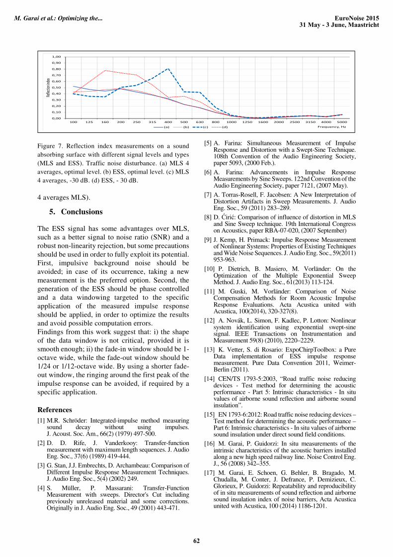
Figure 7. Reflection index measurements on a sound

absorbing surface with different signal levels and types

(MLS and ESS). Traffic noise disturbance. (a) MLS 4

averages, optimal level. (b) ESS, optimal level. (c) MLS

4 averages, -30 dB. (d) ESS, - 30 dB.

4 averages MLS).

5. Conclusions

The ESS signal has some advantages over MLS,

such as a better signal to noise ratio (SNR) and a

robust non-linearity rejection, but some precautions

should be used in order to fully exploit its potential.

First, impulsive background noise should be

avoided; in case of its occurrence, taking a new

measurement is the preferred option. Second, the

generation of the ESS should be phase controlled

and a data windowing targeted to the specific

application of the measured impulse response

should be applied, in order to optimize the results

and avoid possible computation errors.

Findings from this work suggest that: i) the shape

of the data window is not critical, provided it is

smooth enough; ii) the fade-in window should be 1-

octave wide, while the fade-out window should be

1/24 or 1/12-octave wide. By using a shorter fade-

out window, the ringing around the first peak of the

impulse response can be avoided, if required by a

specific application.

References

[1] M.R. Schröder: Integrated-impulse method measuring sound decay without using impulses. J. Acoust. Soc. Am., 66(2) (1979) 497-500.

[2] D. D. Rife, J. Vanderkooy: Transfer-function measurement with maximum length sequences. J. Audio Eng. Soc., 37(6) (1989) 419-444.

[3] G. Stan, J.J. Embrechts, D. Archambeau: Comparison of Different Impulse Response Measurement Techniques. J. Audio Eng. Soc., 5(4) (2002) 249.

[4] S. Müller, P. Massarani: Transfer-Function Measurement with sweeps. Director's Cut including previously unreleased material and some corrections. Originally in J. Audio Eng. Soc., 49 (2001) 443-471.

[5] A. Farina: Simultaneous Measurement of Impulse Response and Distortion with a Swept-Sine Technique. 108th Convention of the Audio Engineering Society, paper 5093, (2000 Feb.).

[6] A. Farina: Advancements in Impulse Response Measurements by Sine Sweeps. 122nd Convention of the Audio Engineering Society, paper 7121, (2007 May).

[7] A. Torras-Rosell, F. Jacobsen: A New Interpretation of Distortion Artifacts in Sweep Measurements. J. Audio Eng. Soc., 59 (2011) 283–289.

[8] D. Ćirić: Comparison of influence of distortion in MLS and Sine Sweep technique. 19th International Congress on Acoustics, paper RBA-07-020, (2007 September)

[9] J. Kemp, H. Primack: Impulse Response Measurement of Nonlinear Systems: Properties of Existing Techniques and Wide Noise Sequences. J. Audio Eng. Soc., 59(2011) 953-963.

[10] P. Dietrich, B. Masiero, M. Vorländer: On the Optimization of the Multiple Exponential Sweep Method. J. Audio Eng. Soc., 61(2013) 113-124.

[11] M. Guski, M. Vorländer: Comparison of Noise Compensation Methods for Room Acoustic Impulse Response Evaluations. Acta Acustica united with Acustica, 100(2014), 320-327(8).

[12] A. Novák, L. Simon, F. Kadlec, P. Lotton: Nonlinear system identification using exponential swept-sine signal. IEEE Transactions on Instrumentation and Measurement 59(8) (2010), 2220–2229.

[13] K. Vetter, S. di Rosario: ExpoChirpToolbox: a Pure Data implementation of ESS impulse response measurement. Pure Data Convention 2011, Weimer-Berlin (2011).

[14] CEN/TS 1793-5:2003, “Road traffic noise reducing devices - Test method for determining the acoustic performance - Part 5: Intrinsic characteristics - In situ values of airborne sound reflection and airborne sound insulation”.

[15] EN 1793-6:2012: Road traffic noise reducing devices – Test method for determining the acoustic performance – Part 6: Intrinsic characteristics - In situ values of airborne sound insulation under direct sound field conditions.

[16] M. Garai, P. Guidorzi: In situ measurements of the intrinsic characteristics of the acoustic barriers installed along a new high speed railway line. Noise Control Eng. J., 56 (2008) 342–355.

[17] M. Garai, E. Schoen, G. Behler, B. Bragado, M. Chudalla, M. Conter, J. Defrance, P. Demizieux, C. Glorieux, P. Guidorzi: Repeatability and reproducibility of in situ measurements of sound reflection and airborne sound insulation index of noise barriers, Acta Acustica united with Acustica, 100 (2014) 1186-1201.

0,00

0,10

0,20

0,30

0,40

0,50

0,60

0,70

0,80

0,90

1,00

100 125 160 200 250 315 400 500 630 800 1000 1250 1600 2000 2500 3150 4000 5000

Refle

ction

inde

x

Frequency, Hz(a) (b) (c) (d)



62

optimizing the exponential sine sweep (ess) signal for in ...€¦ · ess signal: (a) with fade-in...

Documents