optimization of the acoustical absorption characteristics of an enclosure

Optimization of the acoustical absorptioncharacteristics of an enclosure

M.Cappelli D'Orazio*, D.M. FontanaUniversita'degli studi di Roma ``La Sapienza'', Dipartimento di Fisica Tecnica, Facolta d'Ingegneria,

via Eudossiana 18, 00184 Rome, Italy.

Received 20 November 1996; received in revised form 11 February 1998; accepted 21 April 1998

Abstract

A method for optimizing the acoustic absorption of a hall characterized by a wide varietyof possible constraints is presented. The method is formulated so that it is possible to obtain atotal optimum solution directly and e�ciently. The method described in the paper is clearlymore e�ective and accurate than the usual ones which are based on exhaustive explorations

involving discrete variations of parameters. Some example applications of the method arereported. # 1998 Elsevier Science Ltd. All rights reserved.

1. Introduction

Well de®ned values of the reverberation time as a function of frequency arenecessary but not su�cient to obtain `a good acoustic performance' in an enclosure[1±6]. Given the reverberation time as a function of the frequency, the calculation ofthe absorption necessary for each frequency band, is very simple as long as theassumptions of the statistical acoustics are considered to hold. Less easy from anoperational point of view is the speci®cation of the most suitable materials and theamounts necessary for the purpose.If such calculations are performed by a trial and error procedure they are rather

time consuming. As a result several authors have been induced to study some com-putational procedures [4±6]. Since multiple solutions between the assigned allow-able limits are possible, `optimization' methods have been proposed.Among the above cited works it is possible to ®nd the use of methods that are

hardly suitable for generalization [5]. The sum of the squares of the di�erencesbetween the reverberation time obtained and the desired values is assumed as theobjective function to be minimized.

Applied Acoustics 57 (1999) 139±162

0003-682X/99/$Ðsee front matter # 1998 Elsevier Science Ltd. All rights reserved.

PII: S0003-682X(98)00021-8

* Corresponding author.

Actually, these di�erences are not introduced as those between obtained anddesired values but, after the de®nition of a tolerance range (e.g. plus or minus 10%),the di�erence is considered equal to zero in the case that the obtained value is insidethe tolerance range and equal to the distance between the obtained value and thenearest limit of the range, if outside.In our opinion this kind of function cannot be considered suitable for representing

the absorption quality of an enclosure. Since it is necessary to consider reverberationphenomena (speech intelligibility, musical rhythms) as well as acoustical distortion(modi®cation of the acoustic spectrum), it is important that the desired values ofreverberation time should be speci®ed for each frequency or frequency band. In thisrespect it is clear that an important di�erence in one band can cause a sizeabledecrease of the overall acoustical quality, while giving rise to a relatively low valueof a cumulative totalizing indicator.In a di�erent approach [6], the method of discretization of the allowed values of

the independent variables has been adopted and, successively, all the possible com-binations of the allowable values of the variables in accordance with the imposedconstraints have been analyzed.However, such a procedure increases in complexity with increase in the number of

the variables and/or the decrease of the width of the discretization intervals andtherefore the improvement of the requested approximation.The scope of the present work is to show how the problem of achieving an opti-

mized solution for the correction of the acoustic absorption of a hall (also for con-ditions very variable as far as the possible limits and the optimization criteria areconcerned), can be formulated as a problem of linear programming or can beconnected to such a kind of problem. In this way, an optimum solution is achievedby using very e�ective and well known procedures.In addition to solving problems related to the reverberation time, the methods

have been used to solve steadystate problems, such as the de®nition of the optimaltreatment arrangement in order to obtain, in the presence of some ®xed noise sour-ces, the minimum possible level in an assigned weighting curve or the minimumequivalent continuous level.

2. Description of the general problem

2.1. Reverberation time

The problem to be solved can be described as follows: Given an enclosure, a wellde®ned value of the reverberation time for each frequency, has to be obtained. Wewill refer, in the following, to the time estimated on the basis of 60 dB decay (indi-cated as T) making the assumption that the desired values (indicated as T�) areassigned in correspondence with bands of frequency (octaves or third-octaves) indi-vidualized by an ordinator index.A certain number of absorbent materials for each of which the Sabine absorption

coe�cient is known at each frequency band, are available. In order to determine the

140 M.C. D'Orazio, D.M. Fontana/Applied Acoustics 57 (1999) 139±162

optimal combination of the amounts of the surfaces for the di�erent materials,it isnecessary to take into account the constraints.The categories of the constraints are:

1. The installable area of each available kind of materials cannot exceed an upperlimit.

2. The total area that can be installed for one or more groups of materials cannotexceed a given value. For example, materials of low mechanical strength haveto be installed only on the ceiling and on the upper areas of walls. On the otherhand, ¯oor covering materials as well as chairs, if any, are covering the groundarea. Obviously this limits the total area available for possible treatment.

3. The di�erence between the obtained and the desired value of T for each bandof frequency must be limited. Such a limit is necessary when the minimizationof the di�erence is not constituting a target in itself.

As far as optimization criteria are concerned, a very meaningful one is theachievement of a small value of the largest absolute value of the di�erencesbetween T and T� for the di�erent bands. Such a criterion is aimed evidently tooptimize the obtainable result in each band of frequency.

Finally, it is interesting to ®nd the cheapest solution by guaranteeing in themeantime that values of T as near as possible to T� be obtained within assignedtolerances. In such a case, of course, constraints of the third category areabsolutely necessary and the margin for a cost optimization will be as greaterthe larger the allowed tolerance.

2.2. Stead-state problems

Consider an enclosure containing several noise sources with assigned character-istics (power, spectrum, activity in the time).The problem is to lower the enclosure noise level with respect to an assigned

weighting curve, or the equivalent continuous level indicated as (Leq) as much aspossible by means of sound absorbtion. As discussed in Section 2.1, particularmaterials and surfaces are available for the purpose.Consequently, the considerations pertinens to the constraints of ®rst and second

category mentioned earlier remain valid.To evaluate Leq or other estimators, notwithstanding the fact that the power and

spectrum of the noise emitted by each source is variable, we can assume here thatsuch a variability can be schematized as a sequence of steadystate situations, basedon the assumption of the energy additive hypothesis; that is, as a sequence of sourcesof ®xed spectrum and power, active only in de®ned intervals within the consideredobservation time Tobs.

3. Problem formulation

The areas sj of installed surfaces for each of the Nm available materials areassumed to be independent variables. The constraints can be formulated as follows:

M.C. D'Orazio, D.M. Fontana/Applied Acoustics 57 (1999) 139±162 141

3.1. First category constraints

Given Sj, the maximum value of the surface of the jth material that can beinstalled, the ®rst category constraints can be expressed simply as:

sj4Sj j � 1 . . .Nm �1�

3.2. Second category constraints

For each one of the available materials a variable �jg is de®ned, equal to 1 whenthe jth material is part of the gth group and equal to 0 in the other cases.If Rg is the upper limit for the total surface of the gth group of materials, the

constraints of the second category are expressed as

XNm

j�1sj�jg � Rg g � 1 . . .Ng �2�

where Ng is the number of groups with a limited total surface.

3.3. Third category constraints

Suppose that T�k is the desired value for T at the nominal frequency of the kthband (octave, third-octaves, etc.). A limitation could be imposed to the relativevalues of the di�erences jTk ÿ T�kj=T�k. This kind of formulation is signi®cant onlywhen the di�erences are very small in respect of the desired values.For example consider a relative di�erence of 100%. If in excess, it means a value

that is two times the desired one. If in defect, it means a zero value for T. Howeverthese two situations represent radically di�erent acoustic realities notwithstandingtheir characterization by the same value of the di�erence parameter.We believe therefore that it is much more meaningful to characterize the di�erences

between Tk and T�k by means of their ratio Tk=T�k and to put a limit on this ratio:

Tk

Tok

h"�K K � 1 . . .Nb �3a�

Tk

T�K5

1

"ÿk"�k 51 "ÿk 51 �3b�

where Nb is the number of bands considered and the indices + or ÿ refer to lowerand upper limits . Normally the values "k are di�erent for the various bands, inaccordance with the response of the human ear that permits tolerances on T60 thatare higher at low and high frequencies than at the central frequencies (of the audiblespectrum); moreover the deviations tolerated in excess can be di�erent in respect ofthose tolerated in diminution. The situation is represented in Fig. 1 [8].


It can be useful to de®ne the values of "K as a function of the value in the band forwhich the allowed tolerance is the minimum. In general that is the value at thenominal frequency of 2000Hz.If "r represents such a value, it can be stated that:

��ÿk �"�ÿk"r

��ÿk 51

The set of the ratios can be assumed to be known function of frequency (by assign-ing for example trends similar to those of Fig. 1)

"�ÿk � ��ÿk "r k � 1 . . .Nb

and the constraints (3a,b) can be expressed as

Tk

T�k4"r�

�k �30a�

Tk

T�k5

1

"r�ÿk�30b�

Of course in order to satisfy both (30a,b)

"r��ÿk 51 k � 1 . . .Nb

Since �r=1,er 51, also.Such constraints can be expressed as a function of the unknowns sj after assuming

a suitable correlation between the absorption and the reverberation time. Consider,for example, the classical Sabine relation, given:

Fig. 1. Reverberation time as function of frequency. The hatched area shows the range of data as pro-

vided by di�erent authors (source: ref. [8]).


Ak= Increase in absorption for the kth band after treatment of the hall.Ao

k= Absorption for the kth band in the bare hall, excluding air absorption.Aa

k= Absorption due to the air in the hall.A�K= Absorption necessary for the kth band to obtain Tk

* andT�K= Value of the required reverberation time.

Normally, the `bare' hall walls will have a small and quite uniform absorptioncoe�cient. This assumption is made in the present work. In such a case,given ajko,the Sabine absorption coe�cients of the di�erent walls in the kth band and ao therelevant average weighted value, we have:

a�jk � a

�k a

� � A�kP

where � is the total surface area of the hall walls.In such a case we have:

Ak �XNm

j�1sj�ajk ÿ a

�k� �4a�

Where ajk is the Sabine absorption coe�cient of the jth material in the kth band.With respect to the air absorption, we can consider as in [3]:

A�k � 8�kV �4b�

with

V= Hall volume (m3)mk= 85.fk

2 10ÿ10/U (m±1)fk= Nominal frequency of the kth band (Hz)U= Relative humidity in %.

The Sabine relationship may be expressed

Tk � 0:161V

Ak � A�k � Aa

k

�4c�

T�k �0:161V

A�k�4d�

substituting (4a,b,c,d ) into Eqs. (30a) and (30b) gives:XNm

j�1sj�ajk ÿ a

�k� � �A

�k � 8�kVÿ A�k

"r��k

�50 �5a�

XNm

j�1sj�ajk ÿ a

�k� � �A

�k � 8�kVÿ A�k"r�

ÿk �40 �5b�


3.4. Objective functions

3.4.1. Minimum of the maximum deviationWe denote the objective function by OF. We must minimize the greatest of the

deviations obtained at the various frequencies. If we characterize again the deviationbetween Tk and T�k by means of their ratios Tk=T

�k and T�k=Tk, the aim of minimizing

the greatest of the deviations obtained at the various frequencies (section 2.1) isequivalent to requiring that the distances between the curves corresponding to theconstraints of the kind (30a,b) are as small as possible.We consider "r as an additional variable of the problem. In the following this

variable is indicated by '51. Then the problem can be expressed by introducing theconstraints

Tk

T�k4'��k �6a�

Tk

T�k5

1

�'�ÿk ��6b�

with the objective function

OF � ' � min '51 �7�

Eq. (6a,b) can be expressed as functions of sj as for the constraints (3a,b). So wehave:

XNm

j�1sj�ajk ÿ a

�k� ÿ

A�k�k�

:1

'� �A�k � 8�kV�50 �8a�

XNm

j�1sj�ajk ÿ a

�k� ÿ A�k�

ÿk '� �A

�k � 8�kV�40 �8b�

3.4.2. Cost optimizationAssuming that the cost of each material is proportional to its surface area, then, if

Cj is de®ned as the unit cost of the jth material, we have

OF �XNm

j�1sjCj � min �9�

In this case, constraints of the kind (5a,b) are needed as well as (1) and (2).

3.4.3. Minimum level at operating conditionsWe assume that we know the levels Lo

ik in each band due to the ith source,obtained before the treatment, as well as the amount of absorption units for eachband, Ao

k, present before the treatment.


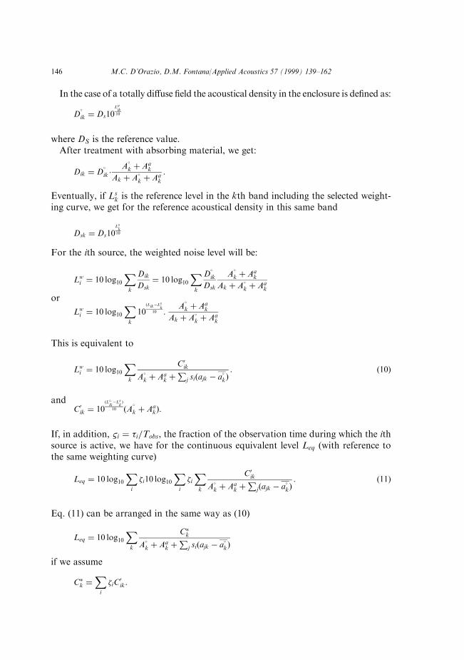
In the case of a totally di�use ®eld the acoustical density in the enclosure is de®ned as:

D�ik � Ds10

Loik10

where DS is the reference value.After treatment with absorbing material, we get:

Dik � D�ik �

A�k � Aa

k

Ak � A�k � Aa

k

:

Eventually, if Lsk is the reference level in the kth band including the selected weight-

ing curve, we get for the reference acoustical density in this same band

Dsk � Ds10Lsk

10

For the ith source, the weighted noise level will be:

Lwi � 10 log10

Xk

Dik

Dsk� 10 log10

Xk

D�ik

Dsk

A�k � Aa

k

Ak � A�k � Aa

k

or

Lwi � 10 log10

Xk

10�LikÿLsk

10 :A�k � Aa

k

Ak � A�k � Aa

k

This is equivalent to

Lwi � 10 log10

Xk

C0ikA�k � Aa

k �P

j si�ajk ÿ a�k�: �10�

andC0ik � 10

�L�ikÿLs

k�

10 �A�k � Aak�:

If, in addition, &i � �i=Tobs, the fraction of the observation time during which the ithsource is active, we have for the continuous equivalent level Leq (with reference tothe same weighting curve)

Leq � 10 log10Xi

�i10 log10Xi

�iXk

C0ikA�k � Aa

k �P

j�ajk ÿ a�k�: �11�

Eq. (11) can be arranged in the same way as (10)

Leq � 10 log10Xk

C�kA�k � Aa

k �P

j si�ajk ÿ a�k�

if we assume

C�k �Xi

�iC0ik:


To obtain the minimum, we can in any case assume as our objective function

OF �Xk

Ck

A�k � Aa

k �P

j si�ajk ÿ a�k�

�12�

with the pertinent de®nition of Ck.

4. Algorithms for optimization

4.1. Reverberation times

The problem of optimizing the maximum deviation between Tk and T�k is descri-bed by the constraints (1), (2), (8a,b) and by the objective function (7). The optimi-zation of the cost is described by Eqs. (1,2) and (5a,b) and by the objective function(9). The constraints expressed by the (1), (2), (5a,b) and the objective function (9) arelinear. The problem of the cost optimization is therefore one of linear programmingand can be solved by using the well known simplex method. The constraint (8a) isnonlinear with respect to the variable. Potentially this may induce a great deal ofcomplexity into the problem solving process. The problem can be overcome bymeans of two di�erent methods. On one hand it is possible to investigate the line-arization of the constraint condition, reaching an approximation that is su�cient forpractical purposes. On the other hand it is possible to ®nd any solution that iscompatible with the constraints conditions (1), (2) and (5a,b) and to search for theminimum value of er for which such a solution exists by iteration.It is to be noted that, notwithstanding the non linearity of the constraint condition

(8a), its structure as well as those of the condition (8b) and the objective function(7), guarantee the existence of a single minimum. As a matter of fact it is immedi-ately evident that if two values, '1 and '2, ('1 < '2) of the objective function arecompatible with both the conditions (8a) and (8b), then any value '14'4'2 iscompatible with (8a,b). The set of values of n, compatible with (8a,b), constitutes acontinuous interval , the lower limit of which is coincident with the minimum for'~ which we search.Of course several combinations of surfaces sj, are possible that give rise to the

unique value of '~. The existence of a unique minimum allows the use of iterationapproximation procedures without the danger of ®nding simply local minima whichwould depend on the values assumed in the ®rst trial.

4.1.1. Linearization of the constraints condition (8a)The constraint condition can be written as

XNm

j�1sj�ajk ÿ a

�k� � A

�k � 8�kV�5A�k

��k:1

'�8c�

where the right hand side depends upon '.


The right hand side of the condition includes the function

��'� � 1

'�13�

that can be substituted by the linear function

l�'� � a� b' �14�Corresponding to the optimal solution ('='~),an error � is present in the estimateof the right hand side of the constraint condition, equal to

� � ��'~� ÿ l�'~� �15�This causes an error in '~, if the constraint is active Di�erent procedures for thelinearization are possible, but the previous considerations indicate some character-istics necessary or convenient for use of (14).If '='~ and the constraint (8c) is valid with the equality sign, (15) indicates it is

necessary that l('~) be coincident with �(') for '='~ and be close to '('~) inthe neighbourhood of the minimum.If, on the other hand '='~ and the constraint (8c) is not active, and, therefore,

(8c) is valid for the > sign, then it is not strictly necessary that l('~)=�('~).However, to maintain the validity of the constraint condition, in the case of substitu-tion of l('~) by '('~), it is very convenient that 8�n� does not overestimate '('~).It should be noted that the properties described above can be attributed to the tangentof l('~) at '='~.We can proceed therefore by assigning for ' a ®rst trial optimal value �.

We put

l�'� � �� d�

d'

� �'

:�'ÿ �� 2

�ÿ '

�2�16�

by indicating the constraint condition (8a) after linearizationXNm

j�1sj�ajk ÿ a

�k� �

A�k��k:1

�2:'� �A�k � 8�kVÿ 2A�k

��k�50 �8d�

and it is possible to solve the linear programming problem (e.g. by the simplexmethod) constituted by (1), (2), (8b,d) and (7). Then, we can ®nd an optimal value ofa second approximation and we can continue until the desired accuracy is reached.Several numerical experiences in connection with actual situations of practical

interest, suggest �=2 for the ®rst trial. In general three iterations are quite su�cientto obtain an accuracy better than 1% and four for an 0.1% accuracy.

4.1.2. Iteration approximationThe problem of ®nding any solution in accordance with the constraint conditions

(1), (2), and (5a,b) can be treated as that of ®nding the minimum cost solution, butputting the unit cost of all the used materials equal to zero. So the problem isreduced to a linear programming problem in a similar way. The method consists insolving the case several times and searching for the smallest value of "r for which it is


possible to ®nd a solution. The search can be accelerated by applying the wellknown bisection law; at the nth iteration, let "1 be the greatest of the proven valuesof "r for which the problem is not solvable (a solution compatible with the con-straints does not exist), and "2 the smallest of the proven value of "r, for which asolution has been found.Then we get

"n�1r � "1 � "22

:

It is possible to push the search up to values "1 and "2 as near as we want.

4.1.3. Comparison between the two methodsThe above described methods have been applied to several cases of practical interest.

The second method involves less time for each iteration since no optimization isinvolved. The procedure is stopped after ®nding the ®rst allowable solution or at theconclusion that a solution does not exist. However to achieve the same accuracy agreater number of iterations is necessary. In both the cases the execution time increaseswith the problem complexity (i.e. the number of materials and constraint conditions).In general the ®rst method is the faster one, with the exception of cases when the

requested accuracy is relatively low (worse than 5%); in which case the second onegives results faster. For problems envisaging about a dozen of materials and three orfour constraints of the second type, accuracies better than 1/10000 can be reached,with a running elapsed time in the order of 10 s on 486 type computers.

4.2. Steady-state problems

The problem of the treatment consistent with the minimum level (or Leq) weightedin a well de®ned way is described by the constraints (1) and (2) and the objectivefunction (12). The objective function is non linear, but is strictly convex and takinginto account that the constraints are linear and are de®ning a convex and closed set,the problem admits a unique minimum point, that is a global minimum. The exis-tence of an unique minimum means that the solution will be independent of thestarting choice and it is possible to follow an iterative method. It is convenient to usea simpli®ed version of the gradient (Franck and Wolfe) method.a. Suppose that a possible solution is found from the rth iteration, s�r� (at the start

we can assume sj=0) and that OF��r�s ) is the relative value of the objective function.b. Solve the linear problem

min :�r� �Xj

@OF

@sj

� �s�r�:Sj

with the constraints (1) and (2). s� the resulting solution and OF�s�) is the relativevalue of the objective function.c. Solve the problem of minimum in the only variable

minfOF �ls�r� � �1ÿ l�s��gso that l� is the solution.


d. Assume as the value of the (r+1)th iteration:

s�r�1� � s�r�l� � s��1ÿ l��and go back to point a. proceeding up to the desired approximation.

4.3. Example applications

For application example no.1, which involved optimization with the respect to thedeviation, the results obtained for the solution of a peculiar problem have beenshown.Fig. 2 gives the global information; case 1a (for T60 see Fig. 2(a) shows the results

obtained by using two materials, case 1b (for T60 see Fig. 2(b) shows the results withsix available materials.

Fig. 2.

Fig. 2a.


Application example no.2 involves optimization with respect to Leq, taking intoconsideration three sources of di�erent spectrum but assuming an equal global levelof 90 dBA.Fig. 3 gives the global information. The cases 2a ,2b and 2c indicate the results

obtained in correspondence with di�erent source activation fractions (equal obser-vation time) of three sources of de®ned spectrum.Referring to the LAeq optimization procedure, it is to be noted that the optimal

solution (the value of LAeq is about the same for the three cases 2a ,2b,2c) has beenobtained by using very di�erent amounts of the same materials for the three cases,given di�erent source situations.By applying the method in a simple and easy way and in view of di�erent opti-

mization targets (reverberation time, LAeq), it is possible to ®nd an optimal solution

Fig. 3.

Fig. 2b.


taking into consideration several constraint conditions in relation with the limitsfor using surfaces of each material and/or group of materials. As far as thereverberation optimization procedure is concerned, it is possible to explore ,asshown in cases 1a and 1b ,the results obtained by implementing the group of mate-rials to be used progressively. Other examples of use of the methods are shown in [9],where a detailed description of the formulation of the cases taken into considerationin accordance with formats required by the routines normally available for thesymplex method utilisation is presented.

5. Conclusions

The proposed method is versatile, e�cient and powerful from a computationalpoint of view. Moreover the use is very simple. The optimal solution is calculated inrelation with either transient state (reverberation time optimization) or steadycondition (min LAeq and equivalence criteria). The optimization takes into accountthe type, the number and the absorption spectrum of all available materials as wellas a wide range of possible constraints. The constraint conditions include limitationson the surfaces to be used for each material and/or group of materials.

Appendix A

A.1. Applicaton example No 1

Sp= ¯oor suface =150m2

Sb= walls surface (with hieght <=2.5m) =125m2

Sa= walls surface (with height >2.5m) =275m2

Ss= ceiling surface =150m2

Stot= overall treatable surface =700m2

V= enclosure volume =1200m3

Materials absorbtion coe�cients

Material no. Material Frequency (Hz)ÿ125 250 500 1000 2000 4000

1 Curtains 0.05 0.06 0.15 0.22 0.29 0.292 Eraclit 0.15 0.18 0.21 0.26 0.38 0.483 Drilled staves 20mm 0.64 0.78 0.6 0.68 0.65 0.654 Drilled staves 40 0.86 0.94 0.76 0.74 0.7 0.725 Moquette 0.1 0.18 0.25 0.3 0.35 0.46 Rubber 0.05 0.05 0.1 0.12 0.12 0.1

Constraints on the available surfaces of the various materials.

. Material no. 1 can be installed on the walls only (tot. height if any).


. Material no. 2,3,4 can be installed on the ceiling and on the high side of thewalls, only.

. Material no. 5 and 6 can be installed on the ¯oor only.We have therefore the constraints:

First type Second types1<=Sa+Sb Sl+s2+s3+s4+s5+s6<=Stots2<=Sa+Ss s2+s3+s4<=Ss+sas3<=Sa+Ss s1+s2+s3+s4<Ss+Sa+Sbs4<=Sa+Ss s5+s6<=Sps5<=Sps6<=Sp

Already existing absorbtion Desired T60 values and tolerancesOctave Pres.Abs Air.Abs. T60 target b+ bÿ125 28.00 0.03 1.35 1.00 1.00250 28.00 0.10 1.12 1.00 1.00500 28.00 0.41 1.01 1.00 1.001000 30.00 1.63 1.00 1.00 1.002000 30.00 6.53 1.00 1.00 1.004000 30.00 26.11 1.01 1.00 1.00

A.2. Case 1a

Optimal solution Basis: Material nos 1,2

Materials to be installedMaterial no. Material Surface (m2)1 Curtains 112.332 Eraclit 425Obtained resultsDeviation factor j=1.539658Octave ActualT60 T60�j�b+ T60/(j�bÿ)125 1.97 2.08 0.88250 1.72 1.72 0.73500 1.43 1.56 0.661000 1.15 1.54 0.652000 0.83 1.54 0.654000 0.66 1.56 0.66

Check of the ®rst type constraintsMaterial no. Material Max. allow. surf. Obtained value1 Curtains 400.0 112.32 Eraclit 425.0 425.0


Check of the second type constraintsMaterial group Max.allow.surf Obtained values1+s2+s3+s4+s5+s6 700 537.33s2+s3+s4 425 425s1+s2+s3+s4 550 537.33s5+s6 150 0

A.3. Case 1b

Optimal solution basis: material nos. 1,2,3,4,5,6Materials to be installedMaterial no. Material Surface(m2)1 Curtians 154.502 Eraclit 03 Drilled staves 20mm 04 Drilled staves 40mm 135.295 Moquette 06 Rubber 150

Obtained resultsDeviation factor j=1.122176Octave Actual T60 T60�j�b+ T60/(j�bÿ)125 1.20 1.51 1.20250 1.12 1.26 1.00500 1.13 1.13 0.901000 1.04 1.12 0.892000 0.99 1.12 0.894000 0.90 1.13 0.90

Check of the ®rst constraintsMaterial no. Material Max allow. surface Obtained value1 Curtains 400.0 154.52 Eraclit 425.0 0.03 Drilled staves 20mm 425.0 0.04 Drilled staves 40mm 425.0 135.35 Moquette 150.0 0.06 Rubber 150.0 150.0

Check of second type constraintsMaterial group Max.allow.surf Obtained values1+s2+s3+s4+s5+s6 700 439.79s2+s3+s4 425 135.29s1+s2+s3+s4 550 289.79s5+s6 150 150.0


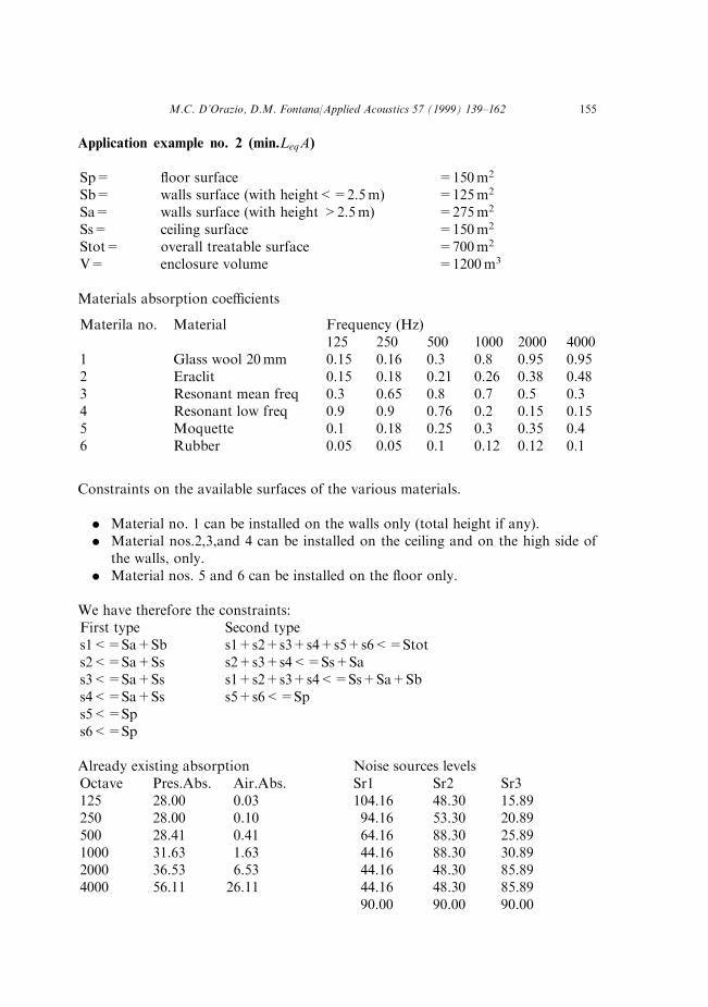
Application example no. 2 (min.LeqA)

Sp= ¯oor surface =150m2

Sb= walls surface (with height<=2.5m) =125m2

Sa= walls surface (with height >2.5m) =275m2

Ss= ceiling surface =150m2

Stot= overall treatable surface =700m2

V= enclosure volume =1200m3

Materials absorption coe�cients

Materila no. Material Frequency (Hz)125 250 500 1000 2000 4000

1 Glass wool 20mm 0.15 0.16 0.3 0.8 0.95 0.952 Eraclit 0.15 0.18 0.21 0.26 0.38 0.483 Resonant mean freq 0.3 0.65 0.8 0.7 0.5 0.34 Resonant low freq 0.9 0.9 0.76 0.2 0.15 0.155 Moquette 0.1 0.18 0.25 0.3 0.35 0.46 Rubber 0.05 0.05 0.1 0.12 0.12 0.1

Constraints on the available surfaces of the various materials.

. Material no. 1 can be installed on the walls only (total height if any).

. Material nos.2,3,and 4 can be installed on the ceiling and on the high side ofthe walls, only.

. Material nos. 5 and 6 can be installed on the ¯oor only.

We have therefore the constraints:First type Second types1<=Sa+Sb s1+s2+s3+s4+s5+s6<=Stots2<=Sa+Ss s2+s3+s4<=Ss+Sas3<=Sa+Ss s1+s2+s3+s4<=Ss+Sa+Sbs4<=Sa+Ss s5+s6<=Sps5<=Sps6<=Sp

Already existing absorption Noise sources levelsOctave Pres.Abs. Air.Abs. Sr1 Sr2 Sr3125 28.00 0.03 104.16 48.30 15.89250 28.00 0.10 94.16 53.30 20.89500 28.41 0.41 64.16 88.30 25.891000 31.63 1.63 44.16 88.30 30.892000 36.53 6.53 44.16 48.30 85.894000 56.11 26.11 44.16 48.30 85.89

90.00 90.00 90.00


A.4. Case 2a

Optimal solution basis: material nos.1,2,3,4,5,6Permanence times of the noise sourcesSr1:t1/Tobs=0.7Sr2:t2/Tobs=0.2Sr3:t3/Tobs=0.1P

ri=1.0

Materials to be installedMaterial no. Material Surface (m2)1 Glass wool 20mm 400.002 Eraclit 0.003 Resonant mean freq. 150.004 Resonant low freq. 0.005 Moquette 150.006 Rubber 0.00

Obtained results LeqA after treatment: 79.1Check of the ®rst type constraintsMaterial no. Material Max allow. surface Obtained value1 Glass wool 20mm 400.0 400.02 Eraclit 425.0 0.03 Resonant mean freq 425.0 150.04 Resonant low freq 425.0 0.05 Moquette 150.0 150.06 Rubber 150.0 0.0

Check of the second type constraintsMaterial group Max allow.surf. Obtained values1+s2+s3+s4+s5+s6 700 700.00s2+s3+s4 425 150.00s1+s2+s3+s4 550 550.00s5+s6 150 150.00

A.5. Case 2b

Optimal solutions basis: material nos.1,2,3,4,5,6Permanence times of the noise sourcesSr1:t1/Tobs=0.1Sr2:t2/Tobs=0.7Sr3:t3/Tobs=0.2P

ri=1.00


Materials to be installedObtained resultsMaterial no. material surface(m2)1 Glass wool 20mm 354.112 Eraclit 0.003 Resonant mean freq. 83.454 Resonant low freq 112.445 Moquette 150.006 Rubber 0.00

LeqA after treatment: 79.1Check of the ®rst type constraintsMaterial no. Material Max allow.surface Obtained value1 Glass wool 20mm 400.0 354.102 Eraclit 425.0 0.03 Resonant mean freq 425.0 83.44 Resonant low freq 425.0 112.45 Moquette 150.0 150.06 Rubber 150.0 0.0

Check of the second type constraints.Material group Max allow. surf Obtaineds1+s2+s3+s4+s5+s6 700 700.00s2+s3+s4 425 195.89s1+s2+s3+s4 550 550.00s5+s6 150 150.00

A.6. Case 2c

Optimal solution basis: material nos.1,2,3,4,5,6Permanence times of the noise sourcesSr1:t1/Tobs=0.2Sr2:t2/Tobs=0.1Sr3:t3/Tobs=0.7P

ri=1.00

Materials to be installedMaterial nos. Material Surface (m2)1 Glass wool 20mm 400.002 Eraclit 0.003 Resonant mean freq. 0.004 Resonant low freq. 150.005 Moquette 150.06 Rubber 0.00


Obtained results LeqA after treatment: 79.8Check of the ®rst type constraintsMaterial no. Material Max allow. surface Obtained value1 Glass wool 20mm 400.0 400.02 Eraclit 425.0 0.03 Resonant mean freq. 425.0 0.04 Resonant low freq. 425.0 150.05 Moquette 150.0 150.06 Rubber 150.0 0.0

Check of the second type constraintsMaterial group Max allow. surf. Obtained values1+s2+s3+s4+s5+s6 700 700.00s2+s3+s4 425 150.00s1+s2+s3+s4 550 550.00s5+s6 150 150.00

Appendix B

B.1. Algorithm for the simplex method

For the use of the simplex method routines, the problem must be presented in asuitable way. In general, if xj are the independent variables (total number Nv) andN1 is the total number of constraints, the problem is formulated as

OF �X

N�j�1 djxj � min �1��

with the ith constraint (i � 1 . . . . . .N1)XN�

j�1 bijxj � Bi50 �2��

or XN�

j�1 bijxj � Bi � 0 �3��

and with the additional conditions

sj50 �4��

(automatically veri®ed in the case under discussion)

Bi50: �5��


In addition it is necessary to characterise the nature of the constraints (equality orinequality). The condition that the known terms Bi are non-negative causes someproblems.If Bi < 0 and the constraint involves equality it is always possible to change the

sign in (3*) thereby satisfying (5*). However if Bi < 0 and the constraint is aninequality it is necessary to go transform to one of equality, by introducing a slackvariable, Yi50 and transforming (2*) into the form

XN�

j�1 bijsj ÿ yi � Bi � 0 �2 � a�

and then change the sign of both members in order to make the known termpositive.It is evident that the constraints (5a,b) and (8b,d) pose such a problem since the

known term can be >,< or = 0 depending upon the amount of the existingabsorbing units in respect of the necessary ones. For such constraints it is necessaryto verify the sign and to introduce the slack variable, if any.To treat all of the constraints homogenously, it is possible to introduce a slack

variable for each of the constraints (5a,b) or (8b,d) (with a zero coe�cient where notnecessary). This causes an increase of the dimension of the matrices to be treated,but simpli®es the algorithm automation. Moreover the initial list must be preparedin the form suitable for the routine to be used. The algorithm for the initial listcompilation is shown below.

B.2. Reduction to standard form

B.2.1. Optimization with respect to the maximum deviationThe process is described by (1), (2), (8b,d), (7).

Where the number of independent variables Nv � Nm � 1� 2Nb

For j � 1 . . .Nm xj � Sj xNm�1 � �For j � Nm � 2 . . .Nm � 2Nb xj � ypp � jÿ �Nm � 2Nb�

The coe�cients with no assigned value are understood to equal zero. By the sameapproach, the constraint, by default, is of inequality.

First category Constraints Second category constraintsj=1. . .Nm; if i � j then bij � ÿ1 i � 1 . . .Nm i � Nm � 1 . . .Nm �Ng; j=1. . .Nm

if i 6�j then bij=0 Bi � Si bij=ÿ�gi where g=iÿNm

Bi=Rg

. 8b.Constraints

. Constraint nature: equality


i � Nm �Ng+1. . .Nm �Ng �Nb bij � ÿA�k�ÿk j � Nm+1

k � iÿ �Nm �Ng� bij=1 j=1. . .Nm+1+K

bij=ajk-a�k j=1. . .Nm Bi=Ak

�+8�kV

. 8d.Constraints

i=Nm+Ng+Nb+1. . .Nm+Ng+2Nb if N<0

k=i-(Nm+Ng+Nb) constraints nature=equality

N=A�k+8�kV -2�

A�k

��k

bij=ÿ(ajkÿa�k� j=1. . .Nm

if N>0 bij=ÿA�k

��k

1�2 j=Nm+1

bij=ajk-a�k j=1. . .Nm bij=1 j=1. . .Nm+Nb+1+K

bij=A�

k

��k

1�2

j � Nm � 1 Bi � ÿNBi � N

. Target function

if j 6� Nm � 1 dj � 0

if j � Nm � 1 dj � ÿ1

B.2.2. Optimization with respect to the costThe process is described by (1),(2) ,(5a,b),(9).

number of independent variables: Nv � Nm � 2Nb

For j � 1 . . .Nm xj � Sj

For j � Nm � 1 . . .Nm � 2Nb xj � ypp � jÿ �Nm � 2Nb�

. First category constraints As in A.2.1.

. Second category contraints As in A.2.1.

. 5a.Constraints

i � Nm �Ng � 1 . . .Nm if N > 0 if N < 0+Ng �Nb

k � iÿ �Nm �Ng� bij � ajk ÿ a�k constraints nature=equalityj � 1 . . .Nm

N � A�k � 8�kVÿ A�k

"r��k

Bi � N bij � ÿ�ajk ÿ a�k�j � 1 . . .Nm

bij � 1 j � Nm � KBi � ÿN


. 5b.Constraintsi � Nm �Ng �Nb . . .Nm if N > 0 if N < 0

+Ng � 2Nb

k � iÿ �Nm �Ng �Nb� costraints nature bij � ÿ�ajk ÿ a�k�=equality j � 1 . . .Nm

N � A�k � 8�kVÿ A�k"r�k bij � ajk ÿ a�k j � 1 . . .Nm Bi � ÿ1

bij � 1 j � Nm �Nb � K

Bi � N

. Target function

di � Cj j � 1 . . .Nm

B.2.3. Minimum leq (for each iteration r > r� 1)

Nv � Nm � 1

j � 1 . . .Nm xj � Sj

xNm�1 � �

. First type constraints

i � 1 . . .Nm if i � jbij � ÿ1Bi � si

. Second type constraints

i � Nm+1. . .Nm �Ng

g � iÿNm bij=-�gjBi � Rg

. Target function

dj � ÿ @0F

@sj

� �s�r�j � 1 . . .Nm

@OF

@sj

� �s�r�� ÿ

Xk

�ajk ÿ a�k�P

i cik�i

A�k � Aa

k �P

j s�r�j �ajk � a

�k�

h i2


B.3. Initial tableThe routine used in the present study requires the compilation of the initial table in

the form:

COL. 1 COL. 2 COL. 3 COL. 4j=1. . .Nv

x$(j)i=1. . .Nl y$(i) aa(i,j) aa(i,Nv+1)i=Nl+1 aa(Nl+1,j)i=Nl+2 aa(Nl+2,j) aa(Nl+2,Nv+1)

where:. Nl is the number of constraints equations: Nl=Nm+Ng+2Nb

. x$(j) is a string identifying the variable to which are the coe�cients of the lowercolumn apply.

. y$(i) is a column of alphanumerical characters identifying the constraintsspeci®ed in the string.

If the constraint is an inequality, the i-th character is the letter `ù'' and the numericalcharacter is the value of the i index. If the constraint has been reduced to anequality ,the character is simply indicated by the letter `ò''.

aa(i,j) =bij for i=1. . .Nl, j=1. . .Nv

aa(i,Nv+1) =Bi for i=1+Nl

aa(Nl+1,j) =cj for j=1. . .Nv

aa(Nl+2,j) � ÿP Nl

i�1 aa(i,j)(i)

For j=1. . .Nv+1 and where: (i)=0 if the constraint ith is of type (identi®er `ù''). �i�=1 if the constraint ith is an equality (identi®er `ò'').

References

[1] Jordan VL. A Group of Objective Acoustical Criteria for Concert Halls. Applied Acoustics

1981;14:253±66.

[2] Gimenez A, Marian A. Analysis and Assessement of Concert Halls. Applied Acoustics 1988;25:235±

41.

[3] Stamac I, Stamac S. Acoustical Response of an Enclosure. J.Audio Eng 1981;9:611±16.

[4] Tzekakis E. . Reverberation Time Prediction Software. Applied Acoustics 1988;24:71±8.

[5] Stamac M, Stamac I. A Method of Computer Aided Optimization of the Absorption in an Enclo-

sure. Acustica 1983;53:91±5.

[6] Ianniello C, Ma�ei L. A Computer Aided Procedure for Selecting the Optional Corrective Absorp-

tion in Rooms. Applied Acoustics 1983;16:455±61.

[7] Muracchini L., Programmazione matematica. Torino: UTET, 1969.

[8] Bruel PER.V, Sound insulation and room acoustics. London: Chapiman and Hall, 1951.

[9] Cappelli D'Orazio M., Fontana DM. Procedimento di ottimizzazione per la correzione delle car-

atteristiche di assorbimento acustico di una sala. Rivista Italiana di Acustica 1992;16(3):67±82.


optimization of the acoustical absorption characteristics of an enclosure

Documents