optimising the operational energy efficiency of an open-pit … · optimising the operational...
TRANSCRIPT

Optimising the operational energy efficiencyof an open-pit coal mine system
by
Samuel Ross PattersonBachelor of Mathematics
Bachelor of Information Technology
CONFIDENTIAL
Submitted in fulfilment of therequirements for the completion of
Doctor of Philosophy
School of Mathematical SciencesScience and Engineering Faculty
Queensland University of Technology
2016

Copyright 2016
Samuel Ross Patterson

Keywords
Optimisation, Integrated Model, Mixed Integer Linear Programming, Hybrid Metaheuristic,Decision Support, Energy Efficiency, Open-pit coal mining.
iii


Abstract
Mining companies are increasingly being challenged to improve energy efficiency, as a methodof reducing both the cost and environmental impact of their operations. This thesis addressesthis issue by investigating the operational energy efficiency of open-pit coal mining. Thepresented approach uses integrated mathematical programming and metaheuristics to modeland optimise operational decisions of mine systems in order to support operators in makingenergy efficient decisions.
Open-pit coal mining methods are reviewed to select the most common subsystems thatrepresent the primary operation and energy consumption; excavation and haulage; stockpile;processing plant; and belt conveyor. Due to the apparent lack of operations research literaturemodelling mine energy efficiency, production system literature is drawn upon by consider-ing an open-pit coal mine as a continuous flow production system. A literature review ofproduction system energy efficiency and how it relates to mine operations is conducted toidentify the most important factors to consider in operational models of mines - asset usageand planning. Integrated modelling is introduced as an effective way of considering all therelevant subsystems and factors together.
Using these findings, a framework for creating an integrated model of an operating open-pit coal mine is proposed and used to formulate an integrated Mixed Integer Linear Program-ming (MILP) model of the four subsystems. A process for applying the framework and modelto new mines is also described.
Accuracy issues are identified with the allocation based formulation of the excavation andhaulage subsystem that was developed based on recent literature. An improved schedulingformulation of the subsystem is developed to overcome these issues. However, the complexityof the improved model means exact methods are unable to provide solutions for practical sizedproblems. A hybrid tabu search and simulated annealing metaheuristic is developed so thatgood quality solutions can be found in reasonable time for practical use.
A case study is conducted of an open-pit coal mine in South East Queensland, Australia.Comprehensive sensitivity analysis is presented to verify and validate that the model andsolution technique provide valuable opportunities for supporting decision makers in theirpursuit of energy efficiency improvements.
v


Contents
Abstract v
List of Figures xi
List of Tables xv
List of Abbreviations xix
Statement of Original Authorship xxi
Acknowledgments xxiii
Chapter 1 Introduction 11.1 Problem outline . . . . . . . . . . . . . . . . . . . . . . . . . . . . . . . . . . . . . . 21.2 Research questions . . . . . . . . . . . . . . . . . . . . . . . . . . . . . . . . . . . . 31.3 Aims, significance and contributions . . . . . . . . . . . . . . . . . . . . . . . . 41.4 Hypotheses . . . . . . . . . . . . . . . . . . . . . . . . . . . . . . . . . . . . . . . . . 51.5 Research approach . . . . . . . . . . . . . . . . . . . . . . . . . . . . . . . . . . . . 51.6 Thesis outline . . . . . . . . . . . . . . . . . . . . . . . . . . . . . . . . . . . . . . . 7
Chapter 2 Literature Review 92.1 Open-pit coal mining . . . . . . . . . . . . . . . . . . . . . . . . . . . . . . . . . . 10
2.1.1 General overview . . . . . . . . . . . . . . . . . . . . . . . . . . . . . . . . 102.1.2 Excavation and haulage . . . . . . . . . . . . . . . . . . . . . . . . . . . . 122.1.3 Processing Plant . . . . . . . . . . . . . . . . . . . . . . . . . . . . . . . . 152.1.4 Stockpiles . . . . . . . . . . . . . . . . . . . . . . . . . . . . . . . . . . . . . 172.1.5 Belt conveyors . . . . . . . . . . . . . . . . . . . . . . . . . . . . . . . . . . 182.1.6 Other subsystems . . . . . . . . . . . . . . . . . . . . . . . . . . . . . . . 182.1.7 Summary . . . . . . . . . . . . . . . . . . . . . . . . . . . . . . . . . . . . . 19
2.2 Production system energy efficiency . . . . . . . . . . . . . . . . . . . . . . . . 192.3 Factors that impact energy efficiency in production systems . . . . . . . . . 23
2.3.1 Asset ownership factors . . . . . . . . . . . . . . . . . . . . . . . . . . . 232.3.2 Asset usage factors . . . . . . . . . . . . . . . . . . . . . . . . . . . . . . . 242.3.3 Human factors . . . . . . . . . . . . . . . . . . . . . . . . . . . . . . . . . 262.3.4 Organisational factors . . . . . . . . . . . . . . . . . . . . . . . . . . . . . 272.3.5 Energy provision factors . . . . . . . . . . . . . . . . . . . . . . . . . . . 282.3.6 Planning factors . . . . . . . . . . . . . . . . . . . . . . . . . . . . . . . . . 282.3.7 External factors . . . . . . . . . . . . . . . . . . . . . . . . . . . . . . . . . 29
2.4 How factors impact the operation of mine subsystems . . . . . . . . . . . . . 302.4.1 Operationally modelled factors . . . . . . . . . . . . . . . . . . . . . . 302.4.2 Excavation and haulage . . . . . . . . . . . . . . . . . . . . . . . . . . . 322.4.3 Processing plant . . . . . . . . . . . . . . . . . . . . . . . . . . . . . . . . 33
vii

viii CONTENTS
2.4.4 Stockpile . . . . . . . . . . . . . . . . . . . . . . . . . . . . . . . . . . . . . 352.4.5 Belt conveyor . . . . . . . . . . . . . . . . . . . . . . . . . . . . . . . . . . 352.4.6 The operational energy model gap . . . . . . . . . . . . . . . . . . . . 36
2.5 Integrated modelling . . . . . . . . . . . . . . . . . . . . . . . . . . . . . . . . . . . 382.6 Solution approaches . . . . . . . . . . . . . . . . . . . . . . . . . . . . . . . . . . . 43
2.6.1 Common solution techniques and hybridisation . . . . . . . . . . . 432.6.2 Solution techniques used in related literature . . . . . . . . . . . . . 46
2.7 Remarks . . . . . . . . . . . . . . . . . . . . . . . . . . . . . . . . . . . . . . . . . . . 50
Chapter 3 Modelling Approach 533.1 Modelling concepts . . . . . . . . . . . . . . . . . . . . . . . . . . . . . . . . . . . 54
3.1.1 Defining the subsystems of a production system . . . . . . . . . . . 543.1.2 Subsystem concepts . . . . . . . . . . . . . . . . . . . . . . . . . . . . . . 553.1.3 Integrating the subsystems . . . . . . . . . . . . . . . . . . . . . . . . . 563.1.4 Capacity . . . . . . . . . . . . . . . . . . . . . . . . . . . . . . . . . . . . . 573.1.5 Operating states . . . . . . . . . . . . . . . . . . . . . . . . . . . . . . . . 583.1.6 Solving . . . . . . . . . . . . . . . . . . . . . . . . . . . . . . . . . . . . . . 59
3.2 Subsystem modelling concepts . . . . . . . . . . . . . . . . . . . . . . . . . . . . 603.2.1 Subsystem model requirements . . . . . . . . . . . . . . . . . . . . . . 613.2.2 Subsystem modelling strategies . . . . . . . . . . . . . . . . . . . . . . 633.2.3 Excavation and haulage subsystem . . . . . . . . . . . . . . . . . . . . 643.2.4 Processing plant subsystem . . . . . . . . . . . . . . . . . . . . . . . . . 663.2.5 Stockpile subsystem . . . . . . . . . . . . . . . . . . . . . . . . . . . . . . 673.2.6 Belt conveyor subsystem . . . . . . . . . . . . . . . . . . . . . . . . . . 67
3.3 Process for applying the integrated model . . . . . . . . . . . . . . . . . . . . . 683.3.1 Gather production system information . . . . . . . . . . . . . . . . . 693.3.2 Outline process flow of system . . . . . . . . . . . . . . . . . . . . . . 743.3.3 Formulate new subsystem model(s) (if required) . . . . . . . . . . . 753.3.4 Apply structural information to integrated model . . . . . . . . . . 763.3.5 Enter subsystem parameter values . . . . . . . . . . . . . . . . . . . . 773.3.6 Enter shift production targets and define operating states . . . . . 803.3.7 Formulate new task(s) (if required) . . . . . . . . . . . . . . . . . . . . 813.3.8 Solve . . . . . . . . . . . . . . . . . . . . . . . . . . . . . . . . . . . . . . . 82
3.4 Remarks . . . . . . . . . . . . . . . . . . . . . . . . . . . . . . . . . . . . . . . . . . . 82
Chapter 4 Integrated Model 854.1 Formulation . . . . . . . . . . . . . . . . . . . . . . . . . . . . . . . . . . . . . . . . 86
4.1.1 Notation . . . . . . . . . . . . . . . . . . . . . . . . . . . . . . . . . . . . . 874.1.2 Parameters . . . . . . . . . . . . . . . . . . . . . . . . . . . . . . . . . . . . 884.1.3 Decision variables . . . . . . . . . . . . . . . . . . . . . . . . . . . . . . . 894.1.4 Objective . . . . . . . . . . . . . . . . . . . . . . . . . . . . . . . . . . . . 904.1.5 Constraints . . . . . . . . . . . . . . . . . . . . . . . . . . . . . . . . . . . 90
4.2 Validation . . . . . . . . . . . . . . . . . . . . . . . . . . . . . . . . . . . . . . . . . 934.2.1 Issues . . . . . . . . . . . . . . . . . . . . . . . . . . . . . . . . . . . . . . . 97
4.3 Remarks . . . . . . . . . . . . . . . . . . . . . . . . . . . . . . . . . . . . . . . . . . 100
Chapter 5 Case Study 1035.1 Apply the integrated model . . . . . . . . . . . . . . . . . . . . . . . . . . . . . . 104
5.1.1 Gather production system information . . . . . . . . . . . . . . . . . 1045.1.2 Outline process flow of system . . . . . . . . . . . . . . . . . . . . . . 1095.1.3 Formulate new subsystem model(s) (if required) . . . . . . . . . . . 111

CONTENTS ix
5.1.4 Apply structural information to integrated model . . . . . . . . . . 1115.1.5 Enter subsystem parameter values . . . . . . . . . . . . . . . . . . . . 1115.1.6 Enter shift production targets and define operating states . . . . . 1115.1.7 Formulate new task(s) (if required) . . . . . . . . . . . . . . . . . . . . 1115.1.8 Solve . . . . . . . . . . . . . . . . . . . . . . . . . . . . . . . . . . . . . . . 111
5.2 Additional constraints . . . . . . . . . . . . . . . . . . . . . . . . . . . . . . . . . 1125.3 Results . . . . . . . . . . . . . . . . . . . . . . . . . . . . . . . . . . . . . . . . . . . 112
5.3.1 Benchmark solution . . . . . . . . . . . . . . . . . . . . . . . . . . . . . 1135.3.2 Demand analysis . . . . . . . . . . . . . . . . . . . . . . . . . . . . . . . . 1155.3.3 Truck analysis . . . . . . . . . . . . . . . . . . . . . . . . . . . . . . . . . 1165.3.4 Issues . . . . . . . . . . . . . . . . . . . . . . . . . . . . . . . . . . . . . . . 117
5.4 Remarks . . . . . . . . . . . . . . . . . . . . . . . . . . . . . . . . . . . . . . . . . . 120
Chapter 6 Improving the Model 1236.1 Excavation and haulage formulation modifications . . . . . . . . . . . . . . . 124
6.1.1 Notation modifications . . . . . . . . . . . . . . . . . . . . . . . . . . . 1256.1.2 Parameter modifications . . . . . . . . . . . . . . . . . . . . . . . . . . . 1256.1.3 Decision variable modifications . . . . . . . . . . . . . . . . . . . . . . 1256.1.4 Constraint modifications . . . . . . . . . . . . . . . . . . . . . . . . . . 1266.1.5 Complexity . . . . . . . . . . . . . . . . . . . . . . . . . . . . . . . . . . . 130
6.2 Validation . . . . . . . . . . . . . . . . . . . . . . . . . . . . . . . . . . . . . . . . . 1316.3 Remarks . . . . . . . . . . . . . . . . . . . . . . . . . . . . . . . . . . . . . . . . . . 133
Chapter 7 Solution Approach 1377.1 Solution technique . . . . . . . . . . . . . . . . . . . . . . . . . . . . . . . . . . . 138
7.1.1 Representation of a solution . . . . . . . . . . . . . . . . . . . . . . . . 1397.1.2 Neighbourhoods . . . . . . . . . . . . . . . . . . . . . . . . . . . . . . . . 1397.1.3 Validation and evaluation of a solution . . . . . . . . . . . . . . . . . 1427.1.4 Constructive heuristic . . . . . . . . . . . . . . . . . . . . . . . . . . . . 1467.1.5 Tabu search . . . . . . . . . . . . . . . . . . . . . . . . . . . . . . . . . . . 1507.1.6 Simulated annealing . . . . . . . . . . . . . . . . . . . . . . . . . . . . . . 1527.1.7 Hybrid technique . . . . . . . . . . . . . . . . . . . . . . . . . . . . . . . 153
7.2 Validation . . . . . . . . . . . . . . . . . . . . . . . . . . . . . . . . . . . . . . . . . 1577.3 Remarks . . . . . . . . . . . . . . . . . . . . . . . . . . . . . . . . . . . . . . . . . . 162
Chapter 8 Results 1658.1 Benchmark solution . . . . . . . . . . . . . . . . . . . . . . . . . . . . . . . . . . . 1668.2 Plan analysis . . . . . . . . . . . . . . . . . . . . . . . . . . . . . . . . . . . . . . . . 1698.3 Asset usage analysis . . . . . . . . . . . . . . . . . . . . . . . . . . . . . . . . . . . 175
8.3.1 Truck analysis . . . . . . . . . . . . . . . . . . . . . . . . . . . . . . . . . 1758.3.2 Cycle time analysis . . . . . . . . . . . . . . . . . . . . . . . . . . . . . . 1778.3.3 Truck waiting time analysis . . . . . . . . . . . . . . . . . . . . . . . . . 1788.3.4 Shovel availability analysis . . . . . . . . . . . . . . . . . . . . . . . . . 179
8.4 Remarks . . . . . . . . . . . . . . . . . . . . . . . . . . . . . . . . . . . . . . . . . . 181
Chapter 9 Discussions and Conclusions 1859.1 Opportunities . . . . . . . . . . . . . . . . . . . . . . . . . . . . . . . . . . . . . . 186
9.1.1 Opportunities for Meandu Mine . . . . . . . . . . . . . . . . . . . . . 1869.1.2 Opportunities for open-pit coal mines . . . . . . . . . . . . . . . . . . 189
9.2 Contributions and implications . . . . . . . . . . . . . . . . . . . . . . . . . . . 2019.2.1 Production system abstraction . . . . . . . . . . . . . . . . . . . . . . . 202

x CONTENTS
9.2.2 Modelling framework . . . . . . . . . . . . . . . . . . . . . . . . . . . . 2039.2.3 Integrated model . . . . . . . . . . . . . . . . . . . . . . . . . . . . . . . . 2059.2.4 Solution technique . . . . . . . . . . . . . . . . . . . . . . . . . . . . . . 2069.2.5 Confirmation of hypothesis . . . . . . . . . . . . . . . . . . . . . . . . 207
9.3 Limitations . . . . . . . . . . . . . . . . . . . . . . . . . . . . . . . . . . . . . . . . 2099.4 Future work . . . . . . . . . . . . . . . . . . . . . . . . . . . . . . . . . . . . . . . . 210
9.4.1 Further analysis of mining systems . . . . . . . . . . . . . . . . . . . . 2109.4.2 Application to other systems . . . . . . . . . . . . . . . . . . . . . . . . 211
9.5 Conclusions . . . . . . . . . . . . . . . . . . . . . . . . . . . . . . . . . . . . . . . . 212
References 215
Appendix A Meandu Mine Model Structure 229
Appendix B Meandu Mine Model Parameters 233B.1 Excavation and haulage . . . . . . . . . . . . . . . . . . . . . . . . . . . . . . . . . 233B.2 Processing plants . . . . . . . . . . . . . . . . . . . . . . . . . . . . . . . . . . . . . 234B.3 Stockpiles . . . . . . . . . . . . . . . . . . . . . . . . . . . . . . . . . . . . . . . . . . 235B.4 Belt conveyors . . . . . . . . . . . . . . . . . . . . . . . . . . . . . . . . . . . . . . . 235
Appendix C Papers published 237

List of Figures
1.1 Research approach . . . . . . . . . . . . . . . . . . . . . . . . . . . . . . . . . . . . 6
2.1 Role of Chapter 2 in the research approach . . . . . . . . . . . . . . . . . . . . 52
3.1 Simple mine map . . . . . . . . . . . . . . . . . . . . . . . . . . . . . . . . . . . . 54
3.2 Mine process flow diagram . . . . . . . . . . . . . . . . . . . . . . . . . . . . . . 55
3.3 Generic subsystem modules . . . . . . . . . . . . . . . . . . . . . . . . . . . . . 60
3.4 Excavation and haulage subsystem overview . . . . . . . . . . . . . . . . . . . 65
3.5 Processing plant subsystem overview . . . . . . . . . . . . . . . . . . . . . . . 66
3.6 Stockpile subsystem overview . . . . . . . . . . . . . . . . . . . . . . . . . . . . 67
3.7 Belt conveyor subsystem overview . . . . . . . . . . . . . . . . . . . . . . . . . 68
3.8 Process for applying the integrated model . . . . . . . . . . . . . . . . . . . . . 69
3.9 Simple hypothetical mine map . . . . . . . . . . . . . . . . . . . . . . . . . . . . 71
3.10 Simple mine process flow diagram . . . . . . . . . . . . . . . . . . . . . . . . . 75
3.11 Role of Chapter 3 in the research approach . . . . . . . . . . . . . . . . . . . . 83
4.1 Driving time differences between trip orders . . . . . . . . . . . . . . . . . . . 98
4.2 Instance 4.01 – Feasible schedule 1 . . . . . . . . . . . . . . . . . . . . . . . . . 99
4.3 Instance 4.01 – Feasible schedule 2 . . . . . . . . . . . . . . . . . . . . . . . . . 99
4.4 Instance 4.01 – Feasible schedule 3 . . . . . . . . . . . . . . . . . . . . . . . . . 100
4.5 Role of Chapter 4 in the research approach . . . . . . . . . . . . . . . . . . . . 101
5.1 Meandu mine satellite image (Maps, 2014) . . . . . . . . . . . . . . . . . . . . 105
5.2 Meandu mine CHPP satellite image (Maps, 2014) . . . . . . . . . . . . . . . . 106
5.3 Meandu mine process flow diagram (Maps, 2014) . . . . . . . . . . . . . . . . 110
5.4 Product demand sensitivity analysis . . . . . . . . . . . . . . . . . . . . . . . . 116
5.5 Truck analysis methodology . . . . . . . . . . . . . . . . . . . . . . . . . . . . . 116
5.6 Effect of taking out each truck from benchmark solution . . . . . . . . . . 117
5.7 Driving time differences between trip orders . . . . . . . . . . . . . . . . . . . 118
xi

xii LIST OF FIGURES
5.8 Example where truck waits for shovel . . . . . . . . . . . . . . . . . . . . . . . 119
5.9 Role of Chapter 5 in the research approach . . . . . . . . . . . . . . . . . . . . 121
6.1 Relationship between Chapters 4 and 6 integrated models . . . . . . . . . . 123
6.2 Instance 4.01 equipment schedule . . . . . . . . . . . . . . . . . . . . . . . . . . 131
6.3 Role of Chapter 6 in the research approach . . . . . . . . . . . . . . . . . . . . 134
7.1 Solution approach structure . . . . . . . . . . . . . . . . . . . . . . . . . . . . . 137
7.2 Solution approach structure . . . . . . . . . . . . . . . . . . . . . . . . . . . . . 139
7.3 Job sequence solution representation after swapping two adjacent jobs
from different states . . . . . . . . . . . . . . . . . . . . . . . . . . . . . . . . . . . 140
7.4 Job sequence solution representation after moving a job backwards or
forwards by one state . . . . . . . . . . . . . . . . . . . . . . . . . . . . . . . . . . 140
7.5 Job sequence solution representation after swapping adjacent jobs from
same state . . . . . . . . . . . . . . . . . . . . . . . . . . . . . . . . . . . . . . . . . 140
7.6 Job sequence solution representation after swapping two random jobs
from same state . . . . . . . . . . . . . . . . . . . . . . . . . . . . . . . . . . . . . . 141
7.7 Job sequence solution representation after swapping two random jobs
from same state . . . . . . . . . . . . . . . . . . . . . . . . . . . . . . . . . . . . . . 141
7.8 Job sequence solution representation after removing a job . . . . . . . . . . 141
7.9 Job sequence solution representation after moving a job to be done by a
different truck . . . . . . . . . . . . . . . . . . . . . . . . . . . . . . . . . . . . . . 141
7.10 Job sequence solution representation after swapping all jobs between two
different trucks . . . . . . . . . . . . . . . . . . . . . . . . . . . . . . . . . . . . . . 142
7.11 Chapter 4 MILP gap % vs instance size measure . . . . . . . . . . . . . . . . . 161
7.12 Role of Chapter 7 in the research approach . . . . . . . . . . . . . . . . . . . . 164
8.1 Benchmark solution schedule . . . . . . . . . . . . . . . . . . . . . . . . . . . . . 168
8.2 Energy consumption of planning analysis scenarios . . . . . . . . . . . . . . 170
8.3 Energy efficiency and stockpile level of scenarios perturbing extraction
targets . . . . . . . . . . . . . . . . . . . . . . . . . . . . . . . . . . . . . . . . . . . . 171
8.4 Energy efficiency and stockpile level of scenarios perturbing product
output . . . . . . . . . . . . . . . . . . . . . . . . . . . . . . . . . . . . . . . . . . . 172
8.5 Energy efficiency vs shovel utilisation for scenarios perturbing extraction
targets . . . . . . . . . . . . . . . . . . . . . . . . . . . . . . . . . . . . . . . . . . . . 174

LIST OF FIGURES xiii
8.6 Equipment schedule with higher shovel utilisation . . . . . . . . . . . . . . . 175
8.7 Effect of taking out each truck from benchmark solution . . . . . . . . . . 176
8.8 Effect of taking out each truck from benchmark solution . . . . . . . . . . 177
8.9 Energy efficiency and shovel utilisation of scenarios perturbing cycle time 178
8.10 Energy efficiency vs truck waiting energy . . . . . . . . . . . . . . . . . . . . 179
8.11 Energy efficiency lost from outage of each shovel in each state . . . . . . . 180
8.12 Role of Chapter 8 in the research approach . . . . . . . . . . . . . . . . . . . . 182
9.1 Role of Section 9.1 in the research approach . . . . . . . . . . . . . . . . . . . 186
9.2 Examples of how model can aid different decision levels . . . . . . . . . . . 192
9.3 Examples of how model can aid different decision levels . . . . . . . . . . . 193
9.4 MineModeller GUI wireframe . . . . . . . . . . . . . . . . . . . . . . . . . . . . 194
9.5 ShiftDashboard target input panel wireframe . . . . . . . . . . . . . . . . . . 196
9.6 ShiftDashboard mine overview wireframe . . . . . . . . . . . . . . . . . . . . 197
9.7 ShiftDashboard excavation and haulage subsystem wireframe . . . . . . . . 198
9.8 EEPlanner workflow diagram . . . . . . . . . . . . . . . . . . . . . . . . . . . . 199
9.9 EEWhatIF workflow diagram . . . . . . . . . . . . . . . . . . . . . . . . . . . . 200
9.10 Contributions delivered using research approach . . . . . . . . . . . . . . . . 202


List of Tables
2.1 Factors considered in mining literature with operational models . . . . . . 31
2.2 Excavation and haulage operational modelling summary . . . . . . . . . . . 32
2.3 Processing plant operational modelling summary . . . . . . . . . . . . . . . . 34
2.4 Stockpile operational modelling summary . . . . . . . . . . . . . . . . . . . . 35
2.5 Belt conveyor operational modelling summary . . . . . . . . . . . . . . . . . 36
2.6 Summary of solution techniques used in related literature . . . . . . . . . . 47
2.7 Summary of solution techniques used in related literature . . . . . . . . . . 48
3.1 Simple example trip driving times (minutes) . . . . . . . . . . . . . . . . . . . 77
3.2 Simple example truck parameters . . . . . . . . . . . . . . . . . . . . . . . . . . 78
3.3 Simple example shovel parameters . . . . . . . . . . . . . . . . . . . . . . . . . . 78
3.4 Simple example processing plant input ratios . . . . . . . . . . . . . . . . . . . 78
3.5 Simple example processing plant parameters . . . . . . . . . . . . . . . . . . . 79
3.6 Simple example stockpile parameters . . . . . . . . . . . . . . . . . . . . . . . . 79
3.7 Simple example belt conveyor parameters . . . . . . . . . . . . . . . . . . . . . 80
3.8 Simple example task list . . . . . . . . . . . . . . . . . . . . . . . . . . . . . . . . . 81
4.1 Simple example task list . . . . . . . . . . . . . . . . . . . . . . . . . . . . . . . . . 94
4.2 Energy consumption (MWh) . . . . . . . . . . . . . . . . . . . . . . . . . . . . . 94
4.3 Total material transferred (tonnes) . . . . . . . . . . . . . . . . . . . . . . . . . . 95
4.4 Truck allocation . . . . . . . . . . . . . . . . . . . . . . . . . . . . . . . . . . . . . 95
4.5 Computational results (simple example instances) . . . . . . . . . . . . . . . . 96
4.6 Case study instance descriptions . . . . . . . . . . . . . . . . . . . . . . . . . . . 96
4.7 Computational results (case study instances) . . . . . . . . . . . . . . . . . . . 97
4.8 Instance 4.01 truck allocations . . . . . . . . . . . . . . . . . . . . . . . . . . . . 97
5.1 Production target tasks . . . . . . . . . . . . . . . . . . . . . . . . . . . . . . . . . 111
5.2 Benchmark energy consumption (MWh) . . . . . . . . . . . . . . . . . . . . . 113
xv

xvi LIST OF TABLES
5.3 Benchmark material transfer over connections (tonnes) . . . . . . . . . . . . 114
5.4 Benchmark truck allocations (# trips) . . . . . . . . . . . . . . . . . . . . . . . . 115
6.1 Instance 4.01 truck allocations . . . . . . . . . . . . . . . . . . . . . . . . . . . . 132
6.2 Problem instance descriptions . . . . . . . . . . . . . . . . . . . . . . . . . . . . 132
6.3 Computational results . . . . . . . . . . . . . . . . . . . . . . . . . . . . . . . . . . 133
7.1 Simple example instance definitions . . . . . . . . . . . . . . . . . . . . . . . . . 158
7.2 Simple example instance objectives . . . . . . . . . . . . . . . . . . . . . . . . . 158
7.3 Simple example instance objective standard deviation . . . . . . . . . . . . . 159
7.4 Simple example instance computation times . . . . . . . . . . . . . . . . . . . 159
7.5 Case study instance definitions . . . . . . . . . . . . . . . . . . . . . . . . . . . . 160
7.6 Case study instance computational results . . . . . . . . . . . . . . . . . . . . . 161
7.7 Case study instance objective standard deviation . . . . . . . . . . . . . . . . 162
7.8 Case study instance computation times . . . . . . . . . . . . . . . . . . . . . . . 162
8.1 Benchmark energy consumption (MWh) . . . . . . . . . . . . . . . . . . . . . 166
8.2 Benchmark material transfer over connections (tonnes) . . . . . . . . . . . . 167
8.3 Benchmark truck allocations (# trips) . . . . . . . . . . . . . . . . . . . . . . . . 168
8.4 Marginal cost per kilotonne of plan target . . . . . . . . . . . . . . . . . . . . . 173
8.5 Marginal cost per kilotonne of plan target . . . . . . . . . . . . . . . . . . . . . 178
A.1 Set of all subsystems . . . . . . . . . . . . . . . . . . . . . . . . . . . . . . . . . . . 229
A.2 Set of excavation and haulage subsystems . . . . . . . . . . . . . . . . . . . . . 229
A.3 Set of processing plant subsystems . . . . . . . . . . . . . . . . . . . . . . . . . . 229
A.4 Set of stockpile subsystems . . . . . . . . . . . . . . . . . . . . . . . . . . . . . . . 230
A.5 Set of belt conveyor subsystems . . . . . . . . . . . . . . . . . . . . . . . . . . . 230
A.6 Sets of connection points, inlets and outlets . . . . . . . . . . . . . . . . . . . . 231
A.7 Set of connections . . . . . . . . . . . . . . . . . . . . . . . . . . . . . . . . . . . . 232
A.8 Set of material types . . . . . . . . . . . . . . . . . . . . . . . . . . . . . . . . . . . 232
B.1 Meandu Mine truck parameters . . . . . . . . . . . . . . . . . . . . . . . . . . . 233
B.2 Meandu Mine shovel parameters . . . . . . . . . . . . . . . . . . . . . . . . . . . 234
B.3 Meandu Mine CHPP input ratios . . . . . . . . . . . . . . . . . . . . . . . . . . 234
B.4 Meandu Mine CHPP parameters . . . . . . . . . . . . . . . . . . . . . . . . . . . 234
B.5 Meandu Mine CHPP stockpile parameters . . . . . . . . . . . . . . . . . . . . 235

LIST OF TABLES xvii
B.6 Meandu Mine belt conveyor parameters . . . . . . . . . . . . . . . . . . . . . . 235


List of Abbreviations
AHP Analytic Hierarchy Process
BC Belt Conveyor
CH Constructive Heuristic
CHPP Coal Handling and Processing Plant
CPP Coal Processing Plant
CVRP Capacitated Vehicle Routing Problem
DES Discrete Event Simulation
DOE Department of Energy
DRET Department of Resources Energy Tourism
EE Energy Efficiency
EEO Energy Efficiency Opportunities
EEX Energy Efficiency Exchange
EWO Enterprise Wide Optimisation
GA Genetic Algorithm
GJ Gigajoules
GUI Graphical User Interface
hr Hour
HSI Horizontal Shaft Impactor
IGVA Industry Gross Value Added
kL Kilolitre
KPI Key Performance Indicator
LOM Life-of-Mine
LP Linear Programming
MILP Mixed Integer Linear Programming
MINLP Mixed Integer Non-Linear Programming
MPC Model Predictive Control
MW Megawatt
MWh Megawatt Hour
xix

xx LIST OF ABBREVIATIONS
NPV Net Present Value
PFD Process Flow Diagram
PP Processing Plant
ROM Run-of-Mine
SA Simulated Annealing
SCOR Supply Chain Operations Reference
SP Stockpile
t Tonne
TS Tabu Search
VSI Vertical Shaft Impactor
WD Waste Dump

QUT Verified Signature


Acknowledgments
Much gratitude goes to my principal supervisor, Professor Erhan Kozan, for taking me on asa student with little experience in the field of operations research and mentoring me throughthe process of learning the field and applying it to this research.
Many thanks also go to my associate supervisor, Professor Paul Hyland, for providinginstrumental thoughts and perspectives on the research itself and the challenge of ensuring itspracticality in industry.
The support of my scholarship provider and employer, Synengco Pty Ltd, is greatly ap-preciated, and has given me the opportunity to continue my studies. Particularly, I wouldlike to thank Don Sands for his countless contributions and commitment to the project.
Sincere appreciation also goes to my close family and friends for being a steady source ofpositive encouragement and support throughout my studies.
Finally, to my editor, Diane Kolomeitz, for copyediting and proofreading services thatcomply with the standards of the Institute of Professional Editors.
SAMUEL ROSS PATTERSON
Queensland University of Technology
2016
xxiii


1Introduction
Mining operations consume high amounts of energy and there are economic, environmental,social and political pressures being placed upon mining companies to improve energy ef-ficiency and reduce their carbon footprint. It is well recognised as an area that requiressignificant attention from both industry and research (Laurence, 2011; Whitmore, 2006).However, the research and development of quantitative models to help tackle the issue isdeficient. This is despite its potential for significant benefit, as seen in many other fields, notleast production systems (Jeon et al., 2014; Li et al., 2014), with relatively low cost comparedto traditional alternatives, such as capital investment in new technology.
This chapter first expands on the challenges facing mining companies to improve energyefficiency in Section 1.1. The research questions that this study focuses on to address theproblem are then presented in Section 1.2. Section 1.3 describes the aims, significance andcontribution of the research. The hypotheses are listed in Section 1.4. Section 1.5 describesthe research approach that was followed to address the questions, achieve the aims and testthe hypotheses. Finally, the remaining chapters of the thesis are outlined in Section 1.6.
1

2 CHAPTER 1. INTRODUCTION
1.1 Problem outline
Energy usage is one area that has become the focus in high cost economies for efficiencyimprovements and cost reductions. Energy consumption of mining operations can havenegative effects on both environmental performance and operating costs (Levesque et al.,2014). Across a wide variety of fields, research has shown that using sound environmentalmanagement techniques can also help improve overall production efficiency (Lindsey, 2011;Ngai et al., 2013), another problem area for Australian mining operations (Lala et al., 2015;Topp et al., 2008).
Coal mining is an important part of the Australian mining industry. Australia was thesecond largest exporter of coal in 2011, a year when exports accounted for approximately86% of the coal mined in Australia (International Energy Agency, 2012). Domestically, it isthe largest fuel source for electricity generation, in 2011-12 an estimated 70% of electricityin Australia came from coal fire power plants (Bureau of Resources and Energy Economics,2013). The importance of coal mining to the Australian economy is clear. However, the eco-nomic viability of coal mines has been put under pressure by falling prices and increased costsin recent years (Lala et al., 2015). This forms an economic challenge for mining companies tobecome more efficient at extracting and processing minerals.
The Australian mining industry accounts for 14% of domestic energy use (AustralianBureau of Statistics, 2010a). Between 1976-77 and 2006-07, energy intensity, expressed asgigajoules per million dollars of Industry Gross Value Added (GJ/$ m IGVA), increased inthe mining industry by 99%, as reported in “Australia’s Environment: Issues and Trends”(Australian Bureau of Statistics, 2010b). Other major industries apart from agriculture haveexperienced decreases in energy intensity over the same period.
This increase can be primarily attributed to the declining grade quality of minerals beingextracted over time (Mudd, 2007). Lower grade quality makes the raw mineral harder toprocess and therefore requires more energy to produce the same amount of product. Alongwith lower ore grades, miners are digging deeper into the ground for raw material, which alsoconsumes more energy.
The Australian Federal Government’s Department of Industry and Science, in associationwith state and territory governments, administers the Energy Efficiency Exchange (EEX),which provides guidance for energy intensive businesses to improve energy efficiency. Miningcompanies are a particular focus of the content provided by EEX, that recommends accurateanalysis and reporting from mining businesses in relation to both the current energy con-sumption and the efforts being made to improve energy efficiency.
The combination of rising energy intensity of the mining industry; increased cost of en-ergy; and increased socio-political pressure for companies to reduce energy consumption andgreenhouse gas emissions; makes energy efficiency an excellent candidate for optimisation.However, as will be explained in Chapter 2, mining literature that uses good practice opera-tions research techniques to address the issue falls behind the more general field of productionsystems. This motivates research into how methods of modelling used for production systemscan be applied to a mining system to support energy efficient decisions.

1.2 Research questions 3
1.2 Research questions
The overarching research question for this study is:
How can the energy efficiency of a mining production system be modelled effectively?
In order to answer this, the following sub-questions are proposed:
1. How can the energy efficiency of mining production systems benefit from an integratedmodelling approach?
(a) Why is improving energy efficiency a concern for mining operations?
(b) How can an open-pit coal mine be considered as a production system?
(c) What factors impact the energy efficiency of a mine?
(d) What are the benefits of using a quantitative optimisation model of energy effi-ciency?
(e) Why take an integrated optimisation approach?
2. What integrated optimisation model of energy efficiency is appropriate for an open-pitcoal mine production system?
(a) What level of detail is required of the model?
(b) Where are the main points of model complexity?
(c) How general should the model be?
(d) What is an appropriate process for applying the model to a real life mine?
3. What solution techniques will be appropriate for solving the model in real-time?
(a) How hard is it to solve the developed model? Is the optimisation NP hard?
(b) Are new techniques required?
(c) What impact do any new solution techniques have on optimality and speed?

4 CHAPTER 1. INTRODUCTION
1.3 Aims, significance and contributions
As stated in the problem outline, increasing energy efficiency is an important goal for amining operation from economic, environmental, social and political perspectives. Tied withan apparent lack of operations research looking optimising energy efficiency of open-pit coalmines, the primary aim of this research project is to:
Identify key factors influencing energy efficiency in open-pit coal mines and developan integrated model that can be used as an energy efficiency decision support tool.
To achieve this aim, a mining operation will be treated as a continuous flow productionsystem and literature from the production system field will be drawn upon. The intent ofthis approach is to provide a substantial academic foundation for using knowledge from theproduction system field to address the problem studied in this thesis. It will also serve as anexample for how to tackle similar problems where research falls behind the methods used inproduction system literature.
Based on these findings, a conceptual framework for developing integrated models of con-tinuous production systems will be contributed. The framework will be based around mod-elling the subsystems of the system separately and connecting them via material mass flowconnections, an approach more commonly seen in the production system field and suggestedby the Australian Government EEO legislation, now under the EEX name (DepartmentResources Energy and Tourism, 2010). Being able to formulate the subsystem models sep-arately will be an important feature of the approach as it allows for distinct differences in theoperation of the subsystems. For example, it allows for a more discrete formulation to modelthe transactional nature of the excavation and haulage subsystem while a more continuousformulation can model the nature of the processing plant operation.
The generalisability of the approach is designed to be a useful contribution for future workand means it can be applied to a wider set of problems than the one specifically consideredin this study. To foster this, a model application process will also be developed to allow foreasy application of the model to new mines, with steps included for extra modelling effortif it is required, an important contribution both for future academic work on the model andfor applying it in practice.
Using the modelling framework and application process, an original integrated formula-tion of a general open-pit coal mine operation will be developed and applied to an operatingmine as a case study. This will be a significant extension upon the current mining literat-ure, where modelling is mainly centred on silo optimisation of subsystems and lacks energyefficiency optimisation models.
As is typical with integrated modelling of operations in other production systems, thecomplexity of the model can become an issue when accurate models are required. The modelwill therefore be analysed with respect to its accuracy and complexity and an innovativesolution technique to overcome the expected complexity will be developed and applied. Thiswill ensure that good quality solutions can be found quickly enough for practical use.

1.4 Hypotheses 5
The case study will be used to verify and validate the developed contributions are signific-ant both academically and practically. The contributions of this study will be evaluated basedthe opportunities they present for supporting decision makers to improve energy efficiency.
1.4 Hypotheses
The hypotheses of this research are as follows:
1. Mining operations can benefit from modelling techniques commonly used in produc-tion systems literature.
2. Integrated modelling is an effective approach to modelling the energy efficiency ofmining production system.
3. Mixed Integer Linear Programming (MILP) is appropriate for formulating an integratedmodel of the energy efficiency of an open-pit coal mine.
4. A complex model is required to accurately model the operation of an integrated open-pit coal mine system, in particular the operation of the trucks.
5. A hybrid metaheuristic-based solution technique is able to overcome complexities inthe model to provide solutions quickly without significant loss of solution quality.
6. The developed model and solution technique can be used as a decision support tool formaking more energy efficient decisions.
1.5 Research approach
The following approach, visualised in Figure 1.1, will be taken to answer the research ques-tions; achieve the aims; provide original contributions with academic and practical signific-ance; and test the hypotheses. As previously explained, open-pit coal mine energy efficiencyas it exists as an issue in the problem domain will first be abstracted to be considered a generalcontinuous flow production system, seen in the top left quadrant of Figure 1.1. Literaturewill be reviewed to confirm the validity of the abstraction and that integrated MILP modellingis an effective method of translating the problem into the solution domain. A modellingframework will then be designed for creating an integrated MILP model of a continuous flowproduction system along with a general process for applying developed integrated models tooperating production systems. This framework will be used to model the specific open-pitcoal mine energy efficiency problem addressed in this research. The top right quadrant ofFigure 1.1 shows these.
As is theorised by hypothesis 4 and 5, it is expected that the developed model will be toocomplex to solve with a commercial solver and a new solution technique will be requiredto find good quality solutions in a reasonable timeframe. A hybrid metaheuristic will bedesigned to achieve this. This is shown in the bottom right quadrant of Figure 1.1.

6 CHAPTER 1. INTRODUCTION
In order to verify and validate the developed methodologies, model and solution tech-nique, an operating mine will be used as a case study. The model application process willbe applied to the mine and a comprehensive sensitivity analysis will be conducted. Usingthis, the research outcomes will be studied with respect to the opportunities it presents forimproving energy efficiency of an open-pit coal mine, particularly as a decision support toolfor operators. This can be seen in the bottom left quadrant of Figure 1.1.
The research approach is structured as an improvement loop to allow the study to iterat-ively progress towards achieving the aims, answering the research questions and testing thehypotheses. It also fosters a path for future work on the problem and other related problems.The next section outlines how two iterations of the research approach have been appliedthroughout the remaining chapters of the thesis.
Figure 1.1. Research approach

1.6 Thesis outline 7
1.6 Thesis outline
Chapter 2 details the literature review conducted to form a basis for the research approach.Open-pit coal mining methods are reviewed to help define the problem and find the mostcommon subsystems of a mine. The general concept of production system energy efficiencyand how a mine can be seen as a production system are described. Factors that impact energyefficiency of production systems in general are presented and how these apply to the four sub-systems is studied. Integrated modelling is then reviewed from literature on both productionsystems and mining. Finally, solution techniques required to solve complex models, similarto the one developed in this study, are reviewed.
Chapter 3 presents the approach developed by this research to devise the integrated model.A framework for modelling subsystems separately and integrating them into a single modelis presented. Conceptual models for each subsystem are then introduced. The developedprocess for applying the integrated model to a mine is also presented.
Chapter 4 then puts these concepts into practice and presents the developed integratedmathematical programming model of a generic open-pit coal mine. Preliminary model val-idation is done using a simple example and some potential drawbacks are highlighted.
Chapter 5 introduces Meandu Mine, an open-pit coal mine in South East Queensland, asa case study. The application process is followed to apply the integrated model to the mineusing information provided in-kind by Downer EDI Mining. Scenario analysis is conductedto further verify and validate the developed model and their results confirm that the issueshighlighted in Chapter 4 emerge in practice.
Chapter 6 presents modifications to the excavation and haulage subsystem formulation inorder to overcome the issues displayed in the previous two chapters. A scheduling formula-tion for the subsystem is presented and the simple example from Chapter 4 is used to verifythat it overcomes the issues found with the allocation formulation. However, the increasedcomplexity of the scheduling formulation is found to make the model NP-hard and cannotbe solved for practical sized problems.
Chapter 7 outlines the solution approach developed to overcome the complexities. Asolution representation, neighbourhoods, evaluation algorithms and constructive heuristicare innovated to aid the application of tabu search and simulated annealing metaheuristicsto deal with the specific complexities of this model. The two metaheuristics will then behybridised in a novel example of how software architecture principles can aid the developmentof efficient and effective solution techniques.
Chapter 8 revisits the case study to provide comprehensive sensitivity analysis with thenew Chapter 6 model, to show that the highlighted issues have been overcome and to verifyand validate that the model and solution technique provide useful results to the problem.
Chapter 9 discusses the findings of the study. The opportunities that the research presentsare examined. It addresses how the hypotheses have been tested and the aims accomplished,to deliver significant contributions from a theoretical and practice perspective. Limitationsand future work are outlined, followed by a conclusion.


2Literature Review
Several key topics are addressed in this literature review in order to establish the relevanceand appropriateness of the proposed approach. Initially, a brief introduction to open-pit coalmining is given in order to classify the most important parts of an open-pit coal mine; thisinventory will be used to define where the logical boundaries of the model in this projectshould be. The concept of a production system is then defined, and the importance of energyefficiency in production systems generally and for mining specifically is discussed. Key factorsthat impact energy efficiency are then selected from production system literature, and papersfrom relevant mining literature that consider them are reviewed. The concept of integratedmodelling with respect to production systems and mines is introduced and reviewed, as it isan effective way to consider all the relevant factors together in one model. Finally, solutiontechniques are reviewed to select ones that are appropriate for finding good quality solutionsto complex integrated models, in reasonable time, for practical use.
9

10 CHAPTER 2. LITERATURE REVIEW
2.1 Open-pit coal mining
Though the overarching research question motivating this study is about mining in general,open-pit coal mining is chosen as a specific form of mining on which to focus. This sectionwill first describe most of the different forms of mining as a way of distinguishing what open-pit coal mining is, then look closely into the most common subsystems that make up anopen-pit coal mining operation. The excavation and haulage fleet, processing plant, stockpileand belt conveyor are analysed in detail to show they are the most common subsystems andserve as a good basis for creating a model to provide operational decision support.
2.1.1 General overview
In general terms, mining is the process of extracting raw geological material from the earth. Itrepresents the primary stage of the majority of industrial supply chains in the modern world.There are many types of materials mined across the world and a wide array of methods thatare used to mine them. Australia’s mining sector comprises a broad spectrum of operationsusing various methods to extract a number of different materials for both domestic use andexport to other countries.
Mines can be classified into two extraction techniques - surface mining and undergroundmining. The type of mine is decided upon through an economic study of the deposit beingextracted (Blackham, 1993; Darling, 2011).
Surface mining involves removing the soil and rock, referred to as overburden, above thedeposit to uncover and extract it, and is used when the deposit is relatively close to the surface.There are several types of surface mining techniques for coal, listed below, which are selectedaccording to what is being mined, where the deposit is and what shape the deposit is (Fung,1981; Kininmonth & Baafi, 2009).
• Strip mining
• Open-pit
• Mountaintop removal
• Highwall
Australian coal most commonly uses either strip or open-pit mining, so mountaintop andhighwall will not be discussed here beyond their brief explanations below.
Strip mining is used when the whole ore body is close to the surface and mostly flatand horizontal. In its most simple form, it involves removing the overburden in a long‘strip’, extracting the exposed mineral seam, then moving along, creating an adjacent seamand placing the overburden from the new strip over the previous strip (Westcott et al., 2009).
Open-pit mines are for less conveniently positioned and shaped deposits of minerals. Insimple terms again, a pit is excavated to follow the mineral seam(s) into the earth and overbur-den must be placed to the side to fill in or partially fill in the pit once the mining is finished(Fung, 1981; Westcott et al., 2009).

2.1 Open-pit coal mining 11
Mountaintop removal is much the same, although, as the name suggests, it is used wherethere is a mountain on top of the deposit. This makes for some distinct differences in theway miners have to handle and store overburden (Fung, 1981). This type of surface mining ismore common in North America.
Finally, in layman’s terms, highwall mining is used when the side of a horizontal mineralseam has been exposed but still has overburden over it. A specific piece of machinery is placedat the exposed end of the seam to extract the seam without the need to remove the overburden(Seib, 2009).
Underground mining involves digging tunnels into the earth to reach the desired materialand is for deposits located deeper in the ground. Depending on the type of material beingextracted, there are many different techniques and configurations of digging the tunnels andgetting the ore out. Hard minerals, such as copper, gold and other metals, use techniquessuch as declines, shafts and adits. Miners of soft minerals, such as coal, use methods such aslongwall and room-and-pillar bines (Darling, 2011).
This research is concerned with open-pit surface mining, and will not investigate under-ground techniques beyond this brief introduction.
Australia is the world’s second largest exporter of coal, after Indonesia, exporting 284.5million tonnes in 2011, which accounts for roughly 86% of the coal mined in Australia in thatyear (International Energy Agency, 2012). Exports are primarily to East Asia. Domestically,it is primarily used as fuel for electricity generation, with an estimated 70% of electricity inAustralia coming from coal fire power plants in 2011-12 (Bureau of Resources and EnergyEconomics, 2013). The majority of coal is mined in the eastern states - Queensland, NewSouth Wales and Victoria - though there are coal mines in all Australian states (Bureau ofResources and Energy Economics, 2012).
Coal is formed as dead biotic material is buried deep into the ground and put under highpressures and temperatures over time (Taylor et al., 2009). Under the various different con-ditions under which it can be placed, there are a number of different types of coal depositswhich can form. These have different chemical makeups, which result in different thermalproperties (Thomas, 2012). Besides electricity generation, coal in its solid state can be usedas a fuel for producing steel and cement and in many other industrial situations where heat isrequired, such as the production of steel and cement.
In Australia, there are two main types of coal that are mined, bituminous and lignite.Bituminous coal, commonly referred to as black coal, is a high quality type of coal. It is minedin Queensland and New South Wales and used domestically for electricity production, steelproduction as well as being exported. Lignite, referred to as brown coal, is lower quality coalwhich is the primary coal mined in the other states, mainly for electricity generation (Hutton& Wootton, 2009).
Depending on the quality of the raw coal being extracted from the ground, and what itsintended use is, a number of processing stages may be required for its sale as product. Raw coalextracted from the ground is known as run-of-mine (ROM) coal; this is the input into what istypically referred to as the Coal Preparation Plant (CPP) or Coal Handling and Preparation

12 CHAPTER 2. LITERATURE REVIEW
Plant (CHPP). In some cases, when high quality coal is being extracted, there may be norequirement for processing before it is sold to the customer; therefore it is common for amine to have a bypass around the CHPP, but as the high quality coal is depleted from thedeposit, processing will be required to bring the quality up to a product level (Darling, 2011;Horrocks et al., 2009).
The basic function of the CHPP is to wash the ROM coal to remove soil and rock, resultingin improved quality. This is also known as beneficiation. ROM coal is usually first crushedto smaller, more consistent sizes, to make for easier and more stable handling and processingsteps downstream. Screening is a process of separating the crushed coal based on size. Thiscan be used at various stages of the overall process if the plant is set up with specific equipmentgroups for processing different particle sizes. Separation parts the coal and rock (rejects) bydistinguishing between them based on density. Before the product coal is stored, the water isremoved from it; this is referred to as dewatering. The rejects can also be dewatered beforethey are discarded as a way of recycling water (Darling, 2011; Horrocks et al., 2009).
Once the coal has been transformed into a product and is ready for sale, there are a numberof different ways of delivering it to the customer. If it is being exported, it will be put on atrain, taken to a port and put on a ship destined for the country to which it is being sold. Ifit is being used domestically, then it may be transported by train to the location where it isbeing used, or, if they are close enough, simply carried on a belt conveyor to the customers(Horrocks et al., 2009; , U.S.).
Energy is consumed in many different ways across an open-pit coal mine. Diesel, petrol,electricity and explosives are the most common sources. Bogunovic et al. (2009) propose asystem for monitoring energy consumption across a mine to help identify areas to focus onwhen making improvements. Kecojevic et al. (2014) also conduct data analysis of energy usageacross an open-pit bituminous coal mine. The study proposes a methodology for investigatingthe relationships between energy production, consumption and cost. For the case studymine it analyses, it finds the diesel sources are the highest energy consumers, while explosivesrepresent the highest energy cost. While the methods of these two papers present significantopportunities to help industry improve energy efficiency, they both only give a picture ofwhere the current energy is being consumed in an operation. They do not provide a way toexamine the impact of any potential improvements.
Now that the general concepts of open-pit coal mining have been introduced, some spe-cifics can be examined to identify the most common subsystems of an open-pit coal mine.Descriptions of how energy is used across the subsystems will be given, along with citationsof literature studying their energy efficiency. This will form the initial basis for the modellingefforts being undertaken in this project.
2.1.2 Excavation and haulage
The system responsible for digging up material from the ground, be it waste or ROM coal,and transporting it to its next location, is referred to here as ‘excavation and haulage’. In itssimplest form, there are two main pieces of equipment, shovels and trucks; grouped together

2.1 Open-pit coal mining 13
they are often referred to as shovel and truck fleets. There are many different types of shovelsand trucks that can be used, depending on a number of factors. It is not uncommon to seetwo fleets of shovels and trucks, one dedicated to removing overburden, the other dedicated toremoving ROM coal (Darling, 2011; Westcott et al., 2009). Currently, trucks and shovels aretypically operated by human employees, though recent technologically advances have enabledremote control of machinery, leading towards a goal of completely autonomous control. Thisis expected to lead to significant improvements in productivity and reductions in operatingcosts (Bellamy & Pravica, 2011).
Truck payload, typically measured in tonnes, varies significantly. Payload can range any-where between 40 to 400 tonnes and is selected based on the size of the mine and the requiredproduction rate (Darling, 2011).
There are two main types of truck frames, rigid and articulated. The difference is thatarticulated trucks are all-wheel drive and are hinged between the cab and trailer, which isused for steering, whereas rigid frame trucks are rear-wheel drive, have conventional front-wheel steering and do not have a hinge between the cab and dump box. Articulated frametrucks are more suited to rough road conditions and tight corners. Rigid frame trucks are themore commonly used type in open-pit coal mining (Darling, 2011; Westcott et al., 2009).
Trucks most commonly unload by tipping their trailer and dumping the material behindthem. This is the most versatile way to unload material. An alternate type of dumpingmechanism is the bottom dump, or belly dump, which has openings underneath the trailerthat unload the material beneath them. This can be useful for dumping directly into a hopperto go onto a belt conveyor into the CHPP (Darling, 2011; Westcott et al., 2009).
The term ‘shovel’ has been used so far to describe the generic piece of equipment thatdigs the material, however when talking about the specifics of equipment, the term ‘shovel’implies a particular type of machinery also known as a front end loader. The other type ofmachinery that is used to load trucks with material is an excavator or digger. The differencebetween these two types of equipment is in how they pick up the material. Front end loaderssit on the same level as the truck, at the bottom of the material they are digging, and scoopthe material up from in front of them and then into the truck. Excavators sit on top of thematerial being removed and scoop it up from below them into the truck on the level below(Fung, 1981; Westcott et al., 2009). Here, for simplicity, the term ‘shovel’ is used to refer toeither type of digging equipment.
The digging equipment is selected in accordance with long-term plans, often known asthe life-of-mine (LOM) plan, and policies for pit design and extraction. Then, once owned,short-term planning and pit design takes into consideration the types of machinery available(White et al., 2009).
Alongside shovels, dozers are used at the pit to service the area, keeping the materialtogether in a form that makes it easy to scoop for the digging equipment and away fromthe driving paths of trucks (Darling, 2011; Norgate & Haque, 2010).
There are a number of other pieces of auxiliary equipment used in the pit to assist with theoperations of the trucks and shovels. Common pieces of equipment include, among others,

14 CHAPTER 2. LITERATURE REVIEW
water trucks for keeping roads wet and dust minimal; mobile refuelling trucks for refuellingtrucks and shovels; sump pumps to drain water out of the bottom of the pit; and floodlightsto light the pit when operating at night (Cairns & Arney, 2009; Norgate & Haque, 2010).These are not covered in detail as part of the scope of this thesis, as they do not perform aprimary function for the mining production system.
The other main piece of machinery, which is often seen in large open-pit coal mines, is thedragline. A dragline is used to remove overburden from above coal. A large bucket suspendedfrom a boom is controlled with ropes and chains to scoop overburden material and place itin more convenient locations for the truck and shovel fleet to handle. While the dragline is avery large piece of equipment that uses a lot of energy and is critical to production, it is veryslow to move and should therefore have its operation planned well in advance of the day-to-day operational decision making process. This, along with the limitations of case study data,is why it is not being explicitly considered in this study; instead it will be implicitly consideredby way of constraints in the model around the current available material for excavating, whichthe dragline has left for the truck and shovel fleet (Fung, 1981; Mirabediny & Baafi, 1998;Westcott et al., 2009).
Both diesel and electricity are sources of energy for the equipment used in the excavationand haulage system. Dozers and trucks both use diesel as a fuel source for their engines. Sometrucks use the diesel to generate power for an electric powertrain, which is more efficient thana conventional diesel engine. Digging equipment can be either diesel powered or electric,smaller shovels and excavators are more typically diesel powered, while large shovels can bepowered by electricity. Draglines are powered by electricity. Electricity to equipment inthe pit is provided by means of a high voltage cable, which can be moved to the location ofshovel or dragline using the electricity. Most auxiliary equipment, such as drainage pumpsand floodlights, use electricity and are often powered by mobile diesel generators (Cairns &Arney, 2009; Darling, 2011; Norgate & Haque, 2010).
Truck operation is one area of focus amongst literature analysing haulage and excavationenergy efficiency. Siami-Irdemoosa & Dindarloo (2015) develop a neural network approachfor creating a prediction model of truck fuel consumption that could be used to comparealternate operating conditions. Kecojevic & Komljenovic (2010) analyse several truck modelsunder different load conditions to find correlation between fuel consumption and engineload and propose opportunities for improved operation. Sahoo et al. (2014) develop a non-linear optimisation model mine road topology and truck dynamics for reducing the fuelconsumption of trucks. Salama et al. (2014) use discrete event simulation and mathematicalprogramming to analyse the energy consumption of alternative haulage methods, includingin-pit conveyors, a long-term, strategic planning decision.
The operation of shovels is also considered in literature. Vukotic & Kecojevic (2014)conduct analysis of shovel energy consumption data to identify the impact that operatorshave on energy efficiency. Awuah-Offei & Frimpong (2007) use dynamic simulation of ashovel to identify the specific operation conditions that yield the highest energy efficiency ofthe equipment.

2.1 Open-pit coal mining 15
2.1.3 Processing Plant
As explained previously, the basic set of processing stages used to get the ROM coal to productquality consists of crushing, screening, washing, separating and dewatering. Each plant isdesigned and configured specifically for the type and quality of coal it is processing and qualityof product required. Coal is sampled and tested for various different properties, which will de-termine how much processing is required, such as its ‘washability’, which, in simple language,defines how much rock is mixed with the coal and dictates how hard washing will be. Then, anengineering effort, much like in any other plant or factory, is undertaken to select the correctequipment and design the material flow to suit the coal and meet various other objectives,like throughput capacity, flexibility, maintainability, and efficiency (Horrocks et al., 2009).
Comminution is the term used to describe the reduction of particle size of solid materials.A crusher is a machine used in the early steps of coal processing, which achieves comminutionby depositing material in a chamber where force is applied to the material to fracture and breakit to a smaller size. This general process can be accomplished in a number of different ways(Napier-Munn & Wills, 2011).
One way the crushing happens is by squeezing the material between two solid surfaces ina funnel type configuration, where the material is crushed into smaller sizes as it falls downto where the surfaces are closer. This is the basic principal behind jaw, gyratory and conecrushers. In a jaw crusher, one surface is fixed, while the other moves back and forth to crushthe material between them both. Gyratory and cone crushers both do this work by havinga moving cone head in the middle of a chamber, set up such that the material is squeezedbetween the chamber and the cone head as it moves (King, 2001; Napier-Munn & Wills, 2011).
Another common way of achieving comminution is with an impact crusher. There aretwo types of impact crushers, horizontal shaft impactors (HSI) and vertical shaft impactors(VSI). Impact crushers are fed material from the top, which falls down onto a rotor, propellingthe material against the hard surface of the side of the chamber with enough force to breakthe material. As their names suggest, the difference between them is in the direction of therotor. Horizontal shaft impactors have the rotor set up with the shaft parallel to the groundlike a car wheel, while vertical shaft impactors have the shaft set up perpendicular with theground, like a helicopter prop citepKing2001, Napier-MunnWills2011.
Mineral sizers or roll crushers are another type of crusher; they typically have two parallelshafts with large teeth on them, which rotate in opposite directions inward to each other,fracturing and breaking the material into a smaller size as it is fed between them citepNapier-MunnWills2011.
Classifying material based on physical size is known as screening. Typically, this involvesa mesh ‘screen’ that, when material is fed over it, splits the material into two sizes by smallerpieces of material falling through the screen and larger pieces remaining on top. This processis useful for recirculating larger material through comminution again to reduce its size or forplants that employ alternate processes for differently sized materials (King, 2001).
Separation techniques are used to classify different grades of coal from the reject material.There are many different types of separation methods, with varying degrees of complexity

16 CHAPTER 2. LITERATURE REVIEW
and accuracy. Gravity can be used to differentiate between densities of coal and rejects. Coalis a low density material compared to rock; the material with density between rock and coalis known as middlings. The cut-off range between what is acceptable, rejected or middlingsis set depending on the quality of the coal being input and what quality is required by thecustomer. Middlings may be discarded or put through extra processing stages to crush orwash them further to get the coal out of them.
A jig is one common type of separator, in which the material is placed in a tank of waterand moved, to allow the dense material to sink to the bottom and less dense material to rise.Early jigs placed the material in a basket that moved up and down. There are many differenttypes of jigs today, which all follow the same basic principal. A Baum jig is an example of oneof these variants; it uses compressed air to disturb the contents of the tank (Horrocks et al.,2009; King, 2001; Napier-Munn & Wills, 2011).
Dense, or heavy, medium separation also uses gravity to separate coal from rejects. Whilejigs use water, dense medium separation, as the name suggests, uses a liquid with a higherdensity than water. Magnetite is often used, mixed with water, to produce this dense liquid.This can be performed in a number of different ways. A common piece of equipment usedto apply dense medium separation to coal is a cyclone. A cyclone is a cone-shaped vessel thathas the material in the dense medium pumped through it at pressure in a tangential direction,causing a vortex. The centrifugal force from the vortex opposing the drag force on the movingparticles causes the particles to be separated, based on their density. Dense medium separationis typically more expensive than other techniques, however it offers finer control over thedensities being separated (Horrocks et al., 2009; King, 2001; Napier-Munn & Wills, 2011).
Finely sized coal can be washed using the floatation technique or with spirals. In thefloatation method, material is fed into a chemical bath where the fine coal floats and bondsto bubbles at the top of the bath, while the rejects sink. The spiral method mixes the finematerial with water and feeds it down a helix; the material is separated based on its densitywhen it is under the centrifugal force. Heavy particles remain in the main flow with the liquid,while lighter particles are pushed outward (Horrocks et al., 2009; King, 2001; Napier-Munn& Wills, 2011).
Dewatering can be performed by a number of different machines. Dewatering screens,centrifuges or cyclones are the common methods these machines implement to remove thewater from the coal or rejects (Horrocks et al., 2009; Napier-Munn & Wills, 2011).
Rejects, or tailings, from the CHPP system are most commonly disposed of to a tailingsdam. The reject material from the CHPP is transported via belt conveyor or pipeline toa manmade dam, or pond, where it is left to settle and separate from the water which isthen removed after time and either disposed of safely or reused. There are a number ofdifferent ways to design dams depending on various characteristics of the environment; thisis not a topic covered in detail in this study as it is a concern for long term planning anddesign rather than operational decision making (Napier-Munn & Wills, 2011; EnvironmentalProtection Agency, 1994).
A coal handling and processing plant contributes a significant portion to the overall energy

2.1 Open-pit coal mining 17
consumption of an operating mine, especially in its comminution processes. Typically, all ofthe equipment used in a CHPP consumes electricity as an energy source (Napier-Munn &Wills, 2011; Norgate & Haque, 2010).
There are numerous papers that look energy efficiency of processing plants and specificequipment within them. Matthews & Craig (2013), Numbi & Xia (2014) and Numbi & Xia(2015) align the processing plant’s operation with the electricity price tariffs to minimise cost.Pothina et al. (2007) develop a model of gyratory crusher energy consumption to identify howblasting impacts the equipment’s energy efficiency, as well as its own operating parameters.
2.1.4 Stockpiles
The handling part of CHPP refers to the storage and transportation of ROM coal, in processmaterial, rejects, water and product coal. Material is most commonly transported via beltconveyor, which will be discussed in the next subsection. Storage locations for the coal beforeand after processing are known as stockpiles. In some circumstances, coal can be stored midprocess; for instance a stockpile may be placed between crushing and washing to separate outthe two processes as a buffer for production smoothing (Horrocks et al., 2009).
While the general concept of a stockpile is quite simple, they can come in many differentforms. Stockpiles are designed to best suit the way they receive material from upstream, whattype of feed is required downstream and the capacities of both up and down stream processes.The general terms for adding to and removing from a stockpile are ‘stacking’ and ‘reclaiming’,respectively.
The most common stockpile is the ROM stockpile, which acts as a buffer between thevariable and discrete nature of dump trucks delivering ROM from the pit, and the continuousdemand rate of the CHPP. The other most common stockpile on a coal mine is the productcoal stockpile, which would typically be fed by a belt conveyor from the CHPP and thenreclaimed for product delivery, such as loading a train. Intermediate stockpiles can exist insidethe CHPP to give finer control over the material flow through the plant. A surge bin is a typeof stockpile that is used in this scenario (Darling, 2011).
In a simple ROM stockpile, stacking will occur by dump trucks unloading onto the side ofthe stockpile and dozers pushing the material into a more compact pile. More sophisticatedstockpiles will employ machines called ‘stackers’ to do this, particularly for large stockpilesand where multiple stockpiles are needed, for different grades. These are machines with alarge boom with a belt conveyor, which move along rail tracks, to stack coal onto the top ofthe stockpile (Darling, 2011).
In most circumstances, material being reclaimed from the stockpile will end up on a beltconveyor for transport to its next location; this can happen in a number of different ways.Similar to a stacker, a ‘reclaimer’ is a large piece of machinery for dealing with large andmultiple stockpiles. Reclaimers are also normally on rail tracks; there are many differentmechanisms that reclaimers can have to remove material from the stockpile and feed it ontothe machine’s belt conveyor, which transports the material to the next location. These canalso be combined with stackers. For smaller, simpler stockpiles, front-end loaders and dozers

18 CHAPTER 2. LITERATURE REVIEW
can be used to push the coal into machines called feeders, which put the dumped coal ontobelt conveyors. Material can also be reclaimed by using special bunkers placed below thestockpile, which give a continuous feed of material onto a tunnelled belt conveyor (Darling,2011).
An issue with large stockpiles of coal is their exothermic heating reaction to oxygen, evenin ambient conditions. In large stockpiles, there is reduced heat loss to the surroundingenvironment and if the exothermic heating outweighs the heat loss, spontaneous combustionof the coal can occur. This is a problem from both safety and economic perspectives (Arisoy& Akgün, 1994; Horrocks et al., 2009).
Stockpiles represent material being double handled. For this reason, they should be ofgreat importance when studying mine energy efficiency. The method of energy consumptionof a stockpile depends on what type of stockpile it is. A stockpile with dozers will, of course,have diesel as its primary energy source. Belt conveyors and surge bins will be powered byelectricity. Stackers and reclaimers are most typically powered by electricity as well (Norgate& Haque, 2010).
2.1.5 Belt conveyors
Belt conveyors are the most common way of transporting coal between different parts of themine once it has been extracted and transported by truck. For instance, from ROM stockpileto processing plant, between machines in the processing plant, or from product stockpile totrain loading facility. In some circumstances, not considered in depth here, belt conveyorsare positioned in the pit to move ore straight to the stockpile or handling plant, removing theneed for trucks to do long trips in and out of the pit (Yardley & Stace, 2008).
Many industries use belt conveyors as an efficient way of transporting material betweenfixed points. Mines of all types have been using belt conveyors to transport material since thelate nineteenth century. Since then, the capacities and carrying distances of belt conveyorsused on mines have increased significantly, though the principles have not changed.
Belt conveyors are most typically powered by electric motors. Various different factorsaffect the energy requirements of belt conveyors. These are mostly static considerations,such as belt design, gradient and distance of the belt, which leaves the amount of materialbeing transported as the main operating variable affecting the energy consumption of thebelt (Yardley & Stace, 2008).
Belt conveyor energy consumption is considered in Luo et al. (2014) where model pre-dictive control for improve energy efficiency is proposed. Zhang & Xia (2011) also addressbelt conveyor energy efficiency by identifying opportunities for improvements under variousoperating conditions.
2.1.6 Other subsystems
Another subsystem employed in the open-pit coal mining production system is the drill andblast activity. This subsystem is responsible for breaking up the ground where overburdenand coal lie, to allow the dragline and loaders to easily scoop and move the material. Arrays

2.2 Production system energy efficiency 19
of holes are drilled, packed with explosives and detonated in areas that are to be excavatedsoon. A number of different considerations have to be made here to design the correct blastfor the material being extracted, such as hardness, safety, cost and the LOM plan. The blastingactivity primarily consumes chemical energy, while the drilling activities consume diesel andelectricity as energy sources (Norgate & Haque, 2010).
While the drilling and blasting subsystem is an important process of the open-pit coalmining production system, much like the dragline, its operation is determined by medium-to-long-term plans and is typically run to give weeks of lead time for the downstream excavationprocesses. This means day-to-day operational decisions don’t have a great impact on theextraction of coal or output of product coal. Therefore it is not explicitly considered as partof the scope of this research project. Instead, it is considered implicitly as a constraint of thesystem through the determination of current availability of material for extraction at the pitfaces entered as production targets.
Another energy-consuming activity, which occurs on open-pit mines but is not consideredin this project, is rehabilitation. This refers to the important process of restoring land to itsoriginal vegetated state. This is an increasingly important duty of mining companies, whichare responsible for minimising the long term impact of their operations on the environment.However, since it does not coincide with the day-to-day operations of the mine extractingmaterial and outputting product, it is not considered at all in this study (Bell & Hannan,2009).
Other activities not mentioned above that can occur in open-pit mines are not consideredin this research project, as it is believed that the primary functional and energy-consumingprocesses of a typical open-pit coal mine have been adequately reflected with the systemdescriptions in this section.
2.1.7 Summary
From the study of open-pit coal mining methods conducted here, the four main subsystemsthat will be used in this research will be excavation and haulage, a processing plant, stockpilesand belt conveyors. Using these subsystems as building blocks to create a representation of amining operation should cover the majority of work done and energy consumed in a typicalopen-pit coal mine and the case study mine examined later in this thesis.
As seen throughout this subsection, there are a number of papers addressing open-pit coalmine energy efficiency of these four subsystems. However, they are all specific to individualsubsystems and therefore only represent opportunities for making silo improvements, ratherthan the integrated ‘whole-of-system’ optimisation that is the aim of this thesis.
2.2 Production system energy efficiency
In its most general form, production systems are defined as organisations that transforminputs, such as materials, personnel, equipment, capital, utilities and information into out-puts, in the form of a product or products (Holstein & Tanenbaum, 2013; Martinich, 1997).
20 CHAPTER 2. LITERATURE REVIEW
Systems can either generate physical goods as their output product, such as manufacturingand mining, or can provide a service as their product. This research is concerned with theformer type of production system output.
Within the physical goods realm of this field, there are three primary methods of produc-tion, listed below (Holstein & Tanenbaum, 2013).
• Flow production
• Batch production
• Project production
Flow production systems are those that process inputs, using a well-defined and mostlyidentical sequence of processing stages. Some examples of industries that exploit this typeof production are the paper, automobile, food, petroleum, metals, mining and electronicsindustries. Flow production systems hold a number of advantages over the other meth-ods, including the increased efficiency through specialised equipment, simplified productionscheduling, easier quality control and reduced requirement for in-process inventory. Somedisadvantages are that the systems are usually not very flexible in producing new producttypes or handling unplanned work or stoppages, and they can also suffer from high initialcosts due to the specialised equipment required (Bellgran & Säfsten, 2010; Martinich, 1997).
There are two main types of the flow production system, discrete and continuous. Discreteflow production systems handle the production of individual units, such as books, trucks ortelevisions, while continuous flow production systems are those that produce an uninterrup-ted flow of output, such as electricity, petroleum or product coal (Bellgran & Säfsten, 2010;Martinich, 1997).
Batch production systems describe the typical setup for an organisation that producesseveral distinct products with different inputs, machines, sequences and processes requiredto produce each different product. This allows for high levels of production flexibility todeal with unpredictable or cyclic demand, but can be more inefficient than a system speciallydesigned for a single product type, and can be harder to optimally plan production (Bellgran& Säfsten, 2010; Holstein & Tanenbaum, 2013; Martinich, 1997).
Organisations which output one-of-a-kind products, such as buildings, highways, pro-totypes or software, generally fall into the category of project production systems. Theseproducts are highly specific to the customer and are therefore typically expensive (Holstein& Tanenbaum, 2013; Martinich, 1997). This type of production system is not consideredfurther in this research.
The most common production systems are batch and flow production systems, which canoften be found in combination with each other. This is sometimes referred to as a Cellularproduction system (Bellgran & Säfsten, 2010; Martinich, 1997). Batch, flow and cellular pro-duction systems are the primary subject of this review when referring to production systems.They are mostly represented in literature by the manufacturing industry. Continuous flowproduction systems are of particular interest, as they are the type of production system a mineis considered as in this study, as will be explained in more detail later.

2.2 Production system energy efficiency 21
Thiede (2012) provides a general input-output definition of energy efficiency of a produc-tion system as the ratio of the system’s output over the total amount of energy input into thesystem. This definition is made to be adaptable to all the various possible combinations ofdifferent outputs that a production system can yield, and suits multiple ways of measuringthe amount of energy being used, such as raw energetic value (joules), the cost of energy oreven the environmental impact (e.g. CO2 emissions). Thiede (2012) asserts that there are twoclear strategies to increase this definition of energy efficiency. Either decrease energy inputfor a proportionally small, or no decrease, in product output or increase production with aproportionally small increase in energy consumption.
In this study, the objective value used for modelling is the denominator of this definition.This is used since the produced output of the system is an expected constraint of the model andis therefore fixed. It also ensures linearity in any case where the product output is a decisionvariable of the model. This means that ‘energy consumption’ is used as the objective withinthe model to represent the study’s overall objective of improving energy efficiency.
On top of these straightforward strategies, depending on the specific implementation ofthe efficiency definition being used, more ways could be devised to improve the energy effi-ciency of a system being studied. For instance, if environment impact or energy cost is beingused, changes to the provision of energy, such as using more renewable or cheaper sources, canimprove efficiency without changing the production output or energy consumption (Yuanet al., 2012).
The manufacturing sector makes up a large portion of energy consumption across theworld (International Energy Agency, 2008). There is a wide range of literature addressingways to both measure and improve energy efficiency in the manufacturing industry (Bunseet al., 2010; Bunse & Vodicka, 2010; Cannata & Taisch, 2010; Dietmair & Verl, 2009; Thiede,2012; Yuan et al., 2012). There are also numerous publications looking at energy efficiency ofa mining operation (Medved et al., 2012; Middelberg et al., 2009; of Energy, 2007), though toa lesser extent than in the wider field of production systems. It is the intention of this projectto draw upon the learnings from production system literature on energy efficiency, to extendupon the less mature field of mining energy efficiency.
Considering an operating mine as a production system has been done in previous relatedwork. Everett (2007) looks at iron ore mining from a production system’s perspective whencreating a decision support system to aid operational decisions to reach target ore qualitieswith minimal rehandling and maximal throughput. Jiu et al. (2013) refer to a coal mineas a production system when developing a model for scheduling equipment maintenanceacross the various subsystems of a coal mine for tactical decision making. Zuñiga et al. (2015)also use the analogy to explain in detail how the supply chain operations reference (SCOR)standardisation framework, commonly used for manufacturing production systems can beapplied to the mining production systems. It finds clear benefit to using the SCOR modelin a mining application, despite the various differences between manufacturing and miningoperations.
Most of the literature on production systems covered in this literature review refers to

22 CHAPTER 2. LITERATURE REVIEW
manufacturing production systems. The primary difference a mining production system hasfrom manufacturing production systems is the uncontrollable variability of the surroundingenvironment. Production systems that depend on their environment, like mines do, areknown as open production systems, whereas typical manufacturing plants that are not highlydependent on their environment are known as closed production systems (Bellgran & Säfsten,2010). It is easy to see how mines are dependent on their environment in many different ways.The main effect is the variability in the material being extracted, the input into the productionsystem. Along with this, the geography of the mine affects the layout of the system in anumber of ways, from haul road distances and gradients to CHPP location, waste dump sites,belt conveyor placement and product delivery methods. Weather also has significant impacton the mine’s production. These factors are considered in more detail and related to energylater in Subsection 2.3.7.
This thesis makes the argument that having such uncontrollable variation in a productionsystem means operational decision making is very important for ensuring the whole systemovercomes the variability to reach production targets efficiently. This forms the motivationfor the approach taken in this research to provide decision support at an operational level,for making improvements to the energy efficiency of a mine by considering it in an openproduction system frame.
Ngai et al. (2013) develop a capability maturity model for energy and utility management,named EUMMM (Energy and Utility Management Maturity Model). EUMMM aims to be acoherent framework for organisations to assess their maturity and guide them to high levelsof energy and utility management maturity. The highest level of maturity in the model is‘optimised’. This level specifies that organisations have strong, well defined, processes forincremental and innovative improvement, with quantitative measures and goals for improve-ment. Performance baselining, systematic data collection, analytic models, technologicalimprovement, causal analysis and resolution management are some of the key processes or-ganisations have to be following to be at the highest level of the model.
The importance of energy efficiency in the manufacturing sector is also realised in Bunseet al. (2010). It provides a framework for measuring improvements to energy efficiency andusing these at the three typical levels of the decision hierarchy of an organisation: strategic,tactical and operational.
Decisions that are made at a strategic level are those that are long-term and mostly business-wide, relating to what markets are going to be targeted, what type of products/services willbe provided from what resources at a high level and the overall structure of the company.The tactical level is about realising the strategic decision made in a medium-term time frame,through decisions on plant layout and capacity; equipment provision and maintenance;product design; and preparing their production. Lastly, operational decisions occur in ashort-term time frame and are about planning and executing production to meet demand andlonger term goals set by the strategic level decision makers. The objectives of operationaldecisions are typically based around productivity and efficiency (Ballou, 2004). In this thesis,operational decisions are modelled in order to provide an accurate picture of mine activity,

2.3 Factors that impact energy efficiency in production systems 23
which can then be used to aid decisions from any of these three levels.
2.3 Factors that impact energy efficiency in production systems
In order to accurately analyse and ultimately make improvements to the energy efficiency ofa production system, using the generic definition for energy efficiency described by Thiede(2012) introduced earlier, all factors that impact on the production output, energy provisionand consumption of the system should be considered. These factors can come from areasacross both the physical process of the production system and the organisation running it.Based on a comprehensive search of production system literature that looks at energy, acatalogue of seven factors has been synthesised to cover the broad range of specific issuesthat are focused upon across the literature. This section reviews the literature that was usedto build the catalogue of factors. The factors will then be used in the next section to formthe basis for what requirements of the model will be needed to provide value to an operatingopen-cut coal mine.
2.3.1 Asset ownership factors
Many papers discuss the impact that informed and attentive asset selection has upon energyefficiency. A number of factors related to the ownership of assets are often considered, suchas the provision of new technologies, maintenance policy, and correct machine capacity.
Göschel et al. (2011) cite replacing machinery and equipment with new, more efficient,technology as a common activity of organisations trying to improve energy efficiency of theirmanufacturing operations. For example, more efficient electric drives, pumps, compressorsand heating/cooling systems are mentioned.
Technology is the first of three dimensional system approaches to environmentally sus-tainable manufacturing proposed by Yuan et al. (2012). Materials and energy are the othertwo dimensions in the devised scheme. The technological aspect of their approach is to createa material and energy flow balanced model of a plant to measure both the material utilisationand energy efficiencies of a production system. This allows for scenario analysis to be con-ducted, investigating the impact that new technologies or changes to process parameters haveon material utilisation or energy efficiency, which can be related back to costs for comparisonagainst one another.
Fleiter et al. (2012) consider in depth the energy saving potentials that new technologiescould have in the pulp and paper industry. A long timeframe approach is used to give anaccurate model of the real saving potentials of each studied technology across the whole sectorin Germany until the year 2035. While the paper and its outcomes are not necessarily aimedat providing short term improvements as are the intentions of this project, they nonethelessshow the large impact that adoption of new technologies can have on energy consumption ina production environment.
Equipment capacity is also a factor that impacts energy efficiency. It can have an effect onboth the individual asset energy efficiency level and the wider system level. Gopalakrishnan

24 CHAPTER 2. LITERATURE REVIEW
et al. (2007) provide examples of types of equipment whereby capacity is an important factorin the energy consumption of the asset. These include chillers; heating, ventilation and airconditioning (HVAC) equipment; and air compressors. When capacity is a major factor ina piece of equipment’s energy efficiency function, the planned utilisation of the equipmentshould be taken into account for equipment provision and then the capacity should be takeninto consideration when actually using it Duflou et al. (2012). The impact of utilisation isconsidered in more detail in the next section.
While the above papers are mainly concerned with the impact capacity has on the indi-vidual equipment’s energy efficiency when it is being run below capacity, the capacity ofassets can impact the overall energy efficiency when it becomes a bottleneck of the overallproduction system (Arinez et al., 2010; Leachman, 1997; Thiede, 2012). This can have animpact on the production output and energy consumption of the system - both the numer-ator and denominator, respectively, of the general definition of production system energyefficiency. This is an important reason to have a whole-of-system model, which takes intoaccount material flow through and capacities of all the components of the system (Ellis et al.,2010; Viere et al., 2011), a concept reviewed further in Section 2.5.
Reliability of the asset should be taken into consideration when purchasing equipment.Aside from the functions the assets are performing in the production system, their main-tenance also impacts their energy consumption and therefore the energy efficiency of thesystem. Arinez et al. (2010) suggest using discrete event simulation (DES) as a generic way ofmodelling and studying production systems in order to find energy efficiency improvements.Maintenance is listed as a key area for investigation, specifically suggesting scenario analysisof the impact on energy consumption that preventative maintenance has.
Önüt & Soner (2007) and Thiede (2012) also list maintenance as an area of opportunity forimproving energy efficiency. The analysis of maintenance activity described in the literatureis primarily concerned with the effect it has on the energy efficiency of the assets beingmaintained, however the energy consumed while maintaining will clearly also have an impacton the overall energy efficiency of the system.
Various different maintenance policies exist with different impacts on the asset reliability(Nakagawa, 2008; Wang & Pham, 2006). Preventive maintenance may result in extra time outof service, but usually will run at a lower risk of a major failure and provides more certaintyabout the equipment availability for planners and operators. These types of maintenancepolicies have rich history in the literature showing many of their benefits (Barlow & Hunter,1960; Cheng-Yi, 2004; Liao, 2012; Mine & Nakagawa, 1977). Maintenance activity will alsohave an impact on the availability of the assets in a production system (Olson, 2007), whichis discussed as a factor in itself in the next section.
2.3.2 Asset usage factors
As briefly introduced in the previous section, both utilisation and availability of the assets in aproduction system impact energy efficiency. The operation and control of equipment is alsoa factor in the asset’s energy consumption and therefore overall system’s energy efficiency.
2.3 Factors that impact energy efficiency in production systems 25
With relation to this project, asset usage, operation and control is a primary consideration,as they make up some of the core controls mining companies have, through operationalplanning and decision making, to improve the energy efficiency of their mines.
The importance of asset capacity on energy efficiency is described in the previous sectionfrom the perspective of asset provision. On the other side of provision decisions, as alludedto earlier, are the decisions around asset utilisation. Over or under utilising an asset is wherethe actual negative impacts on energy efficiency are seen.
Jain et al. (2013) conduct an energy efficiency study across a supply chain and outline sev-eral opportunities for improving energy efficiency by managing machine utilisation. Energyconsumption while in standby or idle is a common area which has contributed to poor energyefficiency across the various subsystems as it is a non-value adding cost. Higher utilisationof assets reduces idle time, which can in turn improve efficiency; shutting down unusedequipment is also a suggested way of reducing idle consumption.
He et al. (2012) highlight the importance of understanding and characterising how assetenergy consumption changes when performing different tasks, including idle, start up andshut down consumption. The paper also mentions the importance of trading off energyconsumption improvement against productivity when considering these decisions aroundasset utilisation. Dietmair & Verl (2009) use similar concepts of machine operating statesto create a profile of asset energy consumption as a robust basis for finding improvements.
Modelling the different ‘operating states’ of each subsystem and its equipment is employedsuccessfully in a number of recent papers on production system energy efficiency (Herrmannet al., 2011; Li et al., 2014; Mousavi et al., 2015; Sproedt et al., 2015). Each finds that significantbenefits to energy efficiency are possible by modelling energy consumption for differentoperating states. Due to its popularity and success, the concept is used in this thesis to describethe model’s time dimension as a series of operating states. This is described in more detail inChapter 3.
Utilisation is also directly related to availability. Since utilisation is typically calculated asa ratio of time used over time available, low availability can be a cause of bottlenecks createdby highly utilised equipment rather than low capacity (Stapelberg, 2009). It is important toconsider these two performance measures at the same time to get the best picture of how theasset is being used and what impact it is having on the whole system.
Smith & Ball (2012) model a production system using material, energy and waste flows as away of improving its energy efficiency, which is a concept applied in this research. Their studylooks at sustainability of a production system, which includes energy efficiency and suggestsreduction of idle time through switching off assets instead of having them in standby, so longas that does not have overly negative impacts on production.
It has already been presented that availability of assets can be related to energy efficiencythough time spent performing maintenance, and the amount of maintenance time is relatedto the reliability of the asset. The previous section explored reliability from the perspectiveof procurement; the way the asset is used will also impact reliability. Operating at variousdifferent loads and under different external conditions will impact the reliability of the asset
26 CHAPTER 2. LITERATURE REVIEW
(Stapelberg, 2009).While the utilisation and availability factors described above are mainly concerned with
overall decisions about when and how much the asset is being used, more detailed decisionsare required once the equipment is in operation. The energy profiling methods from theaforementioned papers, He et al. (2012) and Dietmair & Verl (2009), are also used to gain anunderstanding of how the different operating loads directly impact the operational energyconsumption of each asset.
Operational planning is where these asset operating loads and conditions are consideredand set, and is explored later in Subsection 2.3.6. However, energy is consumed and pro-duction targets are reached when the production system is being run and assets are operating,which is why it is important to consider the actual asset’s operation as a factor when analysingenergy efficiency, especially if plans are not made at particularly high resolutions and manymore operational decisions are required to use the assets. Depending on the type of asset,decisions relating to operation can be quite wide ranging, from automated control systems ofprocessing plants to the human decisions of operators using the equipment.
In this thesis, the link between asset usage and planning factors is described using the oper-ating state concept previously mentioned. Here, a plan is considered as a series of operatingstates of the whole system to partition the time dimension of the model. The subsystems andequipment must then work together in their respective operating states to achieve the overallgoals. Once again, this is described in detail in Chapter 3.
The research in Dietmair & Verl (2009) notes the role of operators and control systems inimpacting energy efficiency. The concept of using the model to assist in ‘online’ operationaldecisions is also suggested for improving energy efficiency, even under unplanned conditions.Cannata & Taisch (2010) and Duflou et al. (2012) also identify control systems as importantto consider when improving energy efficiency.
2.3.3 Human factors
Many of the factors presented here involve a decision making process, which involves humanbehaviour. Humans play important roles in decision making all across organisations, fromstructuring high level strategies to making minute set point adjustments to control systemson operating equipment. Ultimately, humans are responsible for the vast majority of de-cisions made across even the most automated production systems, making their judgementan important factor in achieving energy efficiency, though hard to quantify and analyse.
The importance of human behaviour in improving energy efficiency is highlighted inCagno et al. (2013). The study conducts a critical literature review to find a number ofbehavioural barriers in industry. ‘Bounded rationality’ is one of these barriers, which seeshumans making decisions based on simply satisfying constraints and following rules of thumbthat have worked in the past, rather than striving to search for more optimal decisions.
The manner in which information intended to help with making energy efficiency de-cisions is presented is another factor affecting human behaviour, as identified by Cagno et al.(2013). Other barriers presented in the paper’s literature review are the credibility and trust

2.3 Factors that impact energy efficiency in production systems 27
new technology and information hold with employees; ‘inertia’, which refers to decisionmaking that favours the status quo by “treating gains differently from losses, giving greaterweighting to certain outcomes with respect to those that are uncertain, and minimizing the regret”(p. 293); and finally, the values of the individuals making the decisions can be barriers if theydon’t align with the drivers for improving energy efficiency, such as environmental and cost.
Oskouei & Awuah-Offei (2014) look at how dragline operators at a coal mine impactenergy efficiency. A statistical approach is proposed for identifying the energy efficiency ofeach operator. Using this information, management can focus training efforts on the poorerperforming operators to improve energy efficiency. The impact of coal mine equipmentoperators on energy efficiency is also considered in Vukotic & Kecojevic (2014). In that study,shovel operators a ranked by their impact on energy efficiency, leading towards opportunitiesfor targeted training to improve energy efficiency.
These factors are not considered any further for the development of the models for thisthesis. However, for further work on this research project in converting it into a tool for themining industry, these factors play an important part in making the tool provide valuabledecision support that will be trusted and used by employees.
2.3.4 Organisational factors
Further to the impact that human behaviour and communication has on the ability to beenergy efficient, organisational culture plays a major part in creating the right environment toenable employees to make energy efficient decisions. Positive organisational culture is createdand maintained in various ways. Typically this comes from high level management leading byexample, through creating a focus on energy efficiency by establishing improvement targetsacross the business and investing capital in technology, research and development or bonusesto achieve the targets (Cagno et al., 2013; Rudberg et al., 2013; Thiede, 2012).
Cagno et al. (2013), introduced in the previous section, also look at organisational factorsin their study of barriers to industrial energy efficiency. Where power and responsibilitylies within the organisation, it is listed as a possible barrier if it is placed with departmentsor employees that do not see energy efficiency as a primary consideration when makingdecisions. The ‘culture’ of the organisation is also listed as an important factor in whetherenergy efficiency is harboured or disregarded.
Rudberg et al. (2013) looks at how energy management can be considered by organisationsfrom a strategic perspective. This can be done in a number of ways, such as treating energy asa ‘core’ to the business; investing in long term energy saving measures; establishing an energymanager for the business with the responsibility of improving energy efficiency; participat-ing in government programs that encourage implementing energy management systems orgiving incentives for energy saving initiatives; and centralising the energy planning to allowa company-wide optimisation, rather than sub-optimisation of business units.
As with the human factors, these are not considered any further in this thesis, however,should be considered for future work into making a tool from the developed methodologies,which will be useful for industry.

28 CHAPTER 2. LITERATURE REVIEW
2.3.5 Energy provision factors
Since improving energy efficiency is typically motivated by the opportunity to reduce oper-ating costs and environmental impact, it makes sense that organisations should not only lookat the consumption of energy by their operations, but also at the cost and environmentalimpact of the energy they are purchasing or producing to run the business.
Yuan et al. (2012) consider energy supply as a main part of the energy dimension of theirthree dimensional system approach to improving environmental sustainability in manufactur-ing. The paper suggests a method for conducting a cost benefit analysis of clean energy supply.It then goes on to apply the model to a case study in nano-scale manufacturing, comparingthree clean energy alternatives to the existing fossil fuel-based energy sources being used inthe company, solar photovoltaic, wind and fuel cells, with wind being found to have the bestcost benefit in this case.
A number of other papers discuss this as an area of opportunity to improve sustainabilityand energy efficiency of both the individual organisations and whole supply chains (Duflouet al., 2012; Stich et al., 2012; Thiede, 2012; Zanoni et al., 2013). There is also recognition inthe literature of the differences in energy pricing across different countries and from differentsources, which impact motivation for companies to improve energy efficiency, the specificfocuses they have and decisions they ultimately make.
Since these energy provision factors are based around longer term strategy, they do nottranslate into day-to-day operational decisions and are therefore not being considered in detailfor the model developed in this research.
2.3.6 Planning factors
Ultimately, all energy consumption happens during the actual operation of the system. How-ever, it is the strategic, tactical and operational planning stages that influence the actual op-eration of a production system. It is at these planning stages that the factors relating to assetusage are considered in achieving potential energy efficiency improvements.
Once this is done effectively, actually following through and achieving an energy efficientplan is clearly just as important as creating one. The organisation’s ability to execute energyefficient plans will depend on the factors outlined in Subsection 2.3.3 and Subsection 2.3.4,which should also be included in the planning process. These relationships are well knownand described in the continuous improvement domain as the Plan-Do-Check-Act (PDCA)cycle model (Walton, 1988).
Zanoni et al. (2013) present a mathematical programming model which finds productionrates to minimise energy usage for a two-stage production system with inventory. The paperconducts analysis over several production policy cases and finds that energy has a critical roleto play in production planning.
Duflou et al. (2012) focus on discrete part manufacturing to conduct a detailed analysis ofmethods for improving energy and resource efficiency. A number of their recommendationshighlight the benefit of advanced planning techniques for making energy efficiency improve-ments. In particular, they mention the importance of optimising factory wide planning for
2.3 Factors that impact energy efficiency in production systems 29
making overall reductions to energy consumption. Mousavi et al. (2015) use this concept todevelop an integrated simulation framework for modelling production system energy con-sumption. Two manufacturing case studies are analysed to find significant potential for usingthe framework for making energy efficiency improvements.
Newman et al. (2010) conduct a review of how operations research has been applied tomine planning. The paper reviews decades of literature on open-pit and underground miningfrom strategic, tactical and operational planning perspectives primarily using simulation andoptimisation techniques. The paper lists a more holistic model of the mine as an emerging areafor planning models for reaching overall optimal results rather than sub-optimising individualdecisions from different parts of the mine and organisation. Energy is not mentioned in thereview, suggesting it is an underdeveloped area for planning in the mining industry.
While the aim of the developed methodology from this research is not to produce plansfor the mines being modelled, it is intended to help operators execute their plans in an energyefficient manner. This will be done by taking the existing plan as an ‘input’ and providing sup-port for the operational decisions that get made to meet that plan, from an energy efficiencyperspective. Explaining it using the operating states’ concept introduced in Subsection 2.3.2,the model’s responsibility will be to determine the various subsystem and equipment operat-ing states that are required to meet an overall plan, with minimum energy consumption.
2.3.7 External factors
Depending on the production system, different external factors will apply to varying degrees.This section covers some of the main externalities that can impact mining operations and theirenergy efficiency.
Weather is one of these externalities. For various reasons, not least safety, many minesdo not operate during wet weather, which in turn means equipment utilisation is reduced(Department Resources Energy and Tourism, 2010).
The geographical location and existing layout of the mine also impact energy efficiency.Pit face locations and haul roads play a large part in haulage and excavation subsystem energyusage (Department Resources Energy and Tourism, 2010).
Past decisions, or ‘operational history’, are also externalities that impact energy efficiency(Bruckner et al., 2005), one of which for the coal mining industry is the historical determin-ation of what can be considered economical coal. If previously uneconomical coal has beencovered with overburden, this overburden must be relocated once again to reach the lowergrade coal. Another way this may occur is through the existence of equipment that is notenergy efficient, which relates back to the asset ownership factor. Old decisions based on thelong term planning for the mine may not be optimal for updated plans made under differenteconomic and environmental conditions.
Variability in the grade of material being extracted is another uncontrollable externalfactor that impacts the energy efficiency of a mining operation. As mentioned in the in-troduction, declining material grades is a reason for increased energy intensity (Mudd, 2007).
Product demand is another external factor that can impact energy efficiency in production

30 CHAPTER 2. LITERATURE REVIEW
systems (Zanoni et al., 2013). Uncertainty around demand for the product can lead to changesto the planned operation that may lead to inefficient operation, relating back to the asset usageand planning factors.
2.4 How factors impact the operation of mine subsystems
This section reviews a selection of literature on the four main open-pit coal mining subsys-tems chosen to be modelled, which do not necessarily discuss energy but do cover factorsintroduced in the previous section. The mining literature is used to condense these factorsdown to the most important to operational modelling. Following that, a review of how eachsubsystem has been modelled operationally in the literature is conducted.
2.4.1 Operationally modelled factors
Recent mine modelling literature has been reviewed in order to identify the key factors toconsider when modelling the operation of a mine. The focus for the review was papersexamining quantitative models addressing operational decisions on at least one of the foursubsystems analysed. Traditional operations research simulation and optimisation models, orcombinations of the two, were primarily collected, however, some ‘other’ types mathematicalmodels were also included, such as partial differential equations.
To summarise the findings of the review, compliance matrices have been compiled. Thelegend for the entries in the matrix is as follows: explicit mention is marked with an X, minormention with an M and future work with an F. Table 2.1 shows what factors were consideredin each paper.
The most common factors studied, by far, are asset usage and planning. Asset usagefeatures in all 36 papers, while planning explicitly featured in all but eight of the reviewedpapers. The other factors were all much less prevalent. Energy provision was the next mostfeatured factor with only four explicit mentions. This suggests that asset usage and planningthe most important factors to consider when modelling the operation of a mining productionsystem. Hence, they will be the primary focus of the modelling efforts taken out in this thesisand used to analyse the results of the developed model.

2.4 How factors impact the operation of mine subsystems 31
Table 2.1. Factors considered in mining literature with operational models
Paper Ass
etow
ners
hip
Ass
etus
age
Hum
an
Org
anis
atio
nal
Ene
rgy
prov
isio
n
Plan
ning
Ext
erna
l
Castillo & Cochran (1987) - X - - - X -Soumis et al. (1989) - X - - - X -Li (1990) - X - - - X -Kolonja et al. (1993) - X - - - - -Munirathinam & Yingling (1994) - X - - - X -Everett (1997) - X - - - X -Lebedev & Staples (1998) X X - - - X -Binkowski & McCarragher (1999) - X - - - X MHodouin et al. (2001) - X M - - X -Alarie & Gamache (2002) - X - - - X -Robinson (2004) - X - - - X -Ta et al. (2005) - X - - - X XBlouin et al. (2007) - X - - - M MEverett (2007) - X M - - X -Tie et al. (2007) - X - - - - -Ercelebi & Bascetin (2009) M X - - - X -Middelberg et al. (2009) - X - - X X -Mitra (2009) - X - - - X XArelovich et al. (2010) - X M - - M MMeyer & Craig (2010) - X - - - - -Mohanty & Das (2010) - X - - - - -Remes et al. (2010) - X - - - X -Souza et al. (2010) - X - - - X -Bastos et al. (2011) - X X - - - -Hulthén & Magnus Evertsson (2011) - X - - - M FZhang & Xia (2011) - X - - - X -Hanoun et al. (2013) - X M - - X -Matthews & Craig (2013) - X - - X X -Mena et al. (2013) - X - - - X MTa et al. (2013) - X - - - X -Zhao & Chai (2013) - X - - - X -Luo et al. (2014) - X - - - X -Numbi & Xia (2014) - X - - X X -Sahoo et al. (2014) - X - - - X -Chang et al. (2015) - X - - - X -Numbi & Xia (2014) - X - - X X -

32 CHAPTER 2. LITERATURE REVIEW
2.4.2 Excavation and haulage
In total, 16 of the reviewed papers modelled the operation of the haulage and excavationsubsystem. Productivity, production and cost were the objectives or constraints most mod-elled, with grade and maintenance only considered in few papers. Only one paper consideredenergy as a part of their respective models. All papers considered asset usage factors explicitlyand twelve considered planning factors explicitly. Ten papers contained optimisation models,eight contained simulation models, with three crossing over with both optimisation andsimulation models. Table 2.2 summarises these findings.
Table 2.2. Excavation and haulage operational modelling summary
Paper Sim
.or
Opt
.
Ene
rgy
Cos
t
Prod
uctio
n/
thro
ughp
utG
rade
Mai
nten
ance
Prod
uctiv
ity
Ass
etus
age
Plan
ning
Castillo & Cochran (1987) Sim. - - X - - X X XSoumis et al. (1989) Both - M X - - X X XLi (1990) Opt. - M - - - X X XKolonja et al. (1993) Sim. - - X - - M X -Munirathinam & Yingling (1994) Opt. - X - M - X X XAlarie & Gamache (2002) Opt. - X - - F M X XTa et al. (2005) Opt. - X - - - - X XBlouin et al. (2007) Sim. - - X - - X X MErcelebi & Bascetin (2009) Opt. - X X - - X X XArelovich et al. (2010) Sim. - M - - - X X MSouza et al. (2010) Opt. - M X X - X X XBastos et al. (2011) Sim. - X X - - X X -Ta et al. (2013) Both - X X X M X X XMena et al. (2013) Both - - - - X X X XSahoo et al. (2014) Opt. X - X - - X X XChang et al. (2015) Opt. - - X - - X X X
The primary assets that are used in the haulage and excavation subsystem are trucks andshovels. Most of the recent optimisation models from the literature are equipment allocation-based formulations that provide decision support for managers and operators to assign thetrucks to ‘trips’ between pits and destinations (plants, stockpiles or waste dumps) and shovelsto pits (Mena et al., 2013; Sahoo et al., 2014; Souza et al., 2010; Ta et al., 2013). Truck allocationis by far the most modelled operational decision amongst the papers, while the allocation ofshovels is less featured. The shovels’ slow movement and high criticality to achieving desiredproduction rates means that allocation is more likely dealt with at a medium term decisionmaking level rather than operational.
The asset usage factor is sometimes even more accurately considered by modelling thetruck and shovel fleet heterogeneously (Mena et al., 2013). That is, parameterising equipmentbehaviour on an individual basis from actual performance, rather than considering them allto be the same. This allows the model to more accurately represent the actual operation of

2.4 How factors impact the operation of mine subsystems 33
the subsystem, which leads to results that provide better decision support to the operators.The planning factor is considered in the allocation models through constraints ensuring
that predefined extraction or demand rates are achieved. These rates are typically worked outduring medium and long term (tactical and strategic) planning stages and fed down as targetsfor the actual operation to meet. In this configuration, the plan is considered an input into themodel. Extending upon this concept, more factors from plans are included as inputs in somepapers, such as material grade control, minimum stockpile levels or equipment availability.
While allocation models are popular and provide useful results, they are limited in theirability to provide a very accurate representation of the truck and shovel equipment beha-viours. Since allocation formulation cannot provide sequencing or scheduling informationabout the trips that trucks are making, they cannot guarantee shovel and truck synchronicity.Along with this, the models in the literature only consider constant demand rates and produceallocations for a single, steady ‘operating state’ that the mines work at to meet demand. Noneof the allocation models are integrated with the whole mine system either. These issues aredealt with throughout this thesis.
Chang et al. (2015) is the only paper to present a scheduling MILP model of the truckand shovel operation. The paper bases its formulation on a model of truck scheduling atcontainer terminals (Tang et al., 2014). The model is formulated around a sequencing variablethat decides the order that trucks are loaded by shovels. The constraints ensure that trucksand shovels are synchronised and there is enough driving times between jobs. The objectiveof their model is to maximise revenue of throughput of the subsystem and does not consideroperating costs. It also treats all trucks as equal, which cannot provide an accurate reflectionof actual operation. As with the other models, it also only solves for a single operating stateand is not integrated with other subsystems at the mine.
Due to these limitations and the fact that the Chang et al. (2015) model is the only oneof its kind, the modelling effort in this study will be first based on the more common andestablished allocation model. This is done to make a useful contribution to the allocation for-mulation and highlight its drawbacks in detail before formulating a scheduling model to dealwith them. The allocation formulation will also be used to estimate the quality of schedulingsolutions and aid the solution techniques required to solve the scheduling formulation.
2.4.3 Processing plant
Models of the processing plant subsystem were found in 14 of the reviewed papers. Themajority of explicit model features are related to the production or throughput of the plantand grade of the product being produced by the plant. Energy consumption was explicitlymodelled in four papers, including one that integrated the processing plant with stockpileand belt conveyor decisions Middelberg et al. (2009), and there were minor mentions in sixother papers. The planning factor is considered explicitly in six of the papers that modelledthe processing plant. Optimisation models appeared in five of the papers, simulation mod-els appeared in three, while two presented other types of mathematical models. Table 2.3summarises these findings.

34 CHAPTER 2. LITERATURE REVIEW
Table 2.3. Processing plant operational modelling summary
Paper Sim
.or
Opt
.
Ene
rgy
Cos
t
Prod
uctio
n/
thro
ughp
utG
rade
Mai
nten
ance
Prod
uctiv
ity
Ass
etus
age
Plan
ning
Hodouin et al. (2001) Opt. M M M M M - X XTie et al. (2007) Sim. M M - X - - X -Middelberg et al. (2009) Opt. X M M - - - X XMitra (2009) Opt. M M X X - M X XRemes et al. (2010) Sim. M X X X - - X XMeyer & Craig (2010) Sim. - - X X - - X -Mohanty & Das (2010) Opt. - - - X - - X -Hulthén & Magnus Evertsson (2011) Other M M X M - - X MHanoun et al. (2013) Opt. - - X - - - X XMatthews & Craig (2013) Opt. X X X X - X X XZhao & Chai (2013) Other M - X X - M X XNumbi & Xia (2014) Opt. X X X X - M X XNumbi & Xia (2015) Opt. X X X X - M X X
The most common decision variables considered in the research, which covers the assetusage factor, are the feed rates of raw material and water entering the processing plant. This isbecause they are the main controls that operators have over the operation of the plant. Theseflow rates are usually expressed in tonnes/hour for the raw material or litres/hour for water.The maximum throughput capacity is also considered in models as a constraint on the plant’soperation.
Most of the models reviewed here are intended for automatic control systems, in a modelpredictive control (MPC) methodology. For this reason, many include non-linear equationsto account for the dynamics of the specific circuit being modelled. The non-linearity in-troduced by this level of modelling detail cannot be achieved with MILP and would makeintegrating the subsystem with the rest of the mine difficult. Two papers that model theprocessing plant as part of a whole system model considered the overall load of the plant,rather than the non-linear dynamics of it (Hanoun et al., 2013; Middelberg et al., 2009).The Hanoun et al. (2013) model is limited, however, it treats the plant’s operation as aninput, coming from higher levels of planning, and primarily optimises the handling facilitiesconnected to the plant.
As with the haulage and excavation subsystem, the planning factor is taken into accountin processing plant subsystem models by mainly considering planned targets as inputs tothe model for constraining the operation. Grade quality targets are the most commonlyconsidered planned variable; others also take planned production rates as an input. The twomodels that integrated the processing plant’s operation with other subsystems (Hanoun et al.,2013; Middelberg et al., 2009) included a time dimension in their formulation to allow for mul-tiple operating states. The other three models that explicitly considered energy (Matthews &Craig, 2013; Numbi & Xia, 2014, 2015) also included a time dimension to allow for changes

2.4 How factors impact the operation of mine subsystems 35
in operating state. This indicates the importance that considering changes to operating statehas on energy efficiency.
2.4.4 Stockpile
Eight of the papers contained models of the stockpiles used on a mine. Grade, produc-tion/throughput and cost were the most common model features. Energy was consideredin only one paper (Middelberg et al., 2009), which covers the processing plant, stockpile andconveyor belt subsystems. The planning factor is considered in all of the stockpile subsystempapers. Three papers presented optimisation models of the operation, while two were sim-ulation models and the remaining were other forms of mathematical models. These findingare summarised in Table 2.4.
Table 2.4. Stockpile operational modelling summary
Paper Sim
.or
Opt
.
Ene
rgy
Cos
t
Prod
uctio
n/
thro
ughp
utG
rade
Mai
nten
ance
Prod
uctiv
ity
Ass
etus
age
Plan
ning
Everett (1997) Sim. - M X X - - X XLebedev & Staples (1998) Sim. - X X - M X X XBinkowski & McCarragher (1999) Other - X X X M - X XRobinson (2004) Other - - - X - - X XTa et al. (2005) Opt. - X - - - - X XEverett (2007) Other - X X X - - X XMiddelberg et al. (2009) Opt. X M M - - - X XHanoun et al. (2013) Opt. - M X X M X X X
The operation of the stockpile subsystem is often modelled via inlet and outlet mater-ial flow rates and standard inventory balance equations (Ta et al., 2005; Middelberg et al.,2009). Minimum stockpile levels are often included as a constraint of the subsystem. Sincestockpiling represents double handling, the most efficient operations use a stockpile as littleas possible. However, in practice, they are used as buffers to reduce the risk of an upstreamdisturbance impacting downstream processes. For instance, a minimum level of ROM coalshould be maintained so that any unplanned stoppage in the haulage and excavation fleet doesnot mean the processing plant has to stop operation.
Much like the haulage and excavation and processing plant subsystems, the planning factorfor the stockpile subsystem is considered by having information from the plan as input intothe model. This usually comes in the form of production rate targets and/or material gradetargets.
2.4.5 Belt conveyor
Five of the reviewed papers directly modelled the operation of the conveyor belt subsystemand Table 2.5 summarised the models. Production throughput and productivity were major

36 CHAPTER 2. LITERATURE REVIEW
features of two out of the five papers, while energy featured in Middelberg et al. (2009) andLuo et al. (2014). The planning factor is considered explicitly in all three papers. Optimisationmodelling was used in two papers and one paper used a simulation model.
Table 2.5. Belt conveyor operational modelling summary
Paper Sim
.or
Opt
.
Ene
rgy
Cos
t
Prod
uctio
n/
thro
ughp
utG
rade
Mai
nten
ance
Prod
uctiv
ity
Ass
etus
age
Plan
ning
Lebedev & Staples (1998) Sim. - X X - M X X XMiddelberg et al. (2009) Opt. X M M - - - X XZhang & Xia (2011) Opt. X X M - - - X XHanoun et al. (2013) Opt. - M X X M X X XLuo et al. (2014) Opt. X X M - - - X X
Conveyor belts are modelled relatively simply in the literature. Conveyor belt throughputflow rates is the main variable used to define the operation of the machinery, or even simply abinary variable indicating whether it is in service or not, along with an assumption of a fixedflow rate. They also include maximum capacity of the conveyor belt as a constraint of thesubsystem. Luo et al. (2014) contains the most advanced model by considering nonlinearityof the energy consumption in a MPC approach to reducing the energy consumption whenchanges in operating state occur.
Similarly with the other three subsystems, a plan is taken as input to the operationalmodels for the conveyor belt subsystem as their consideration of the planning factor.
2.4.6 The operational energy model gap
There is a lack of operational optimisation models across the reviewed papers that includeenergy consumption. The apparent gap in research, along with the need for industry to ad-dress the problem, forms the motivation for this research. Only a handful of papers explicitlyconsider energy in their operational models. Here they are reviewed to gain an insight intohow this research will contribute to the area with original and substantial contributions.
Luo et al. (2014) demonstrate significant improvements to belt conveyor energy efficiencyby applying MPC. They highlight the operational decision making level as an important areafor practical application of the approach. The results only demonstrate a silo optimisationof a single subsystem instance, and do not study the impact on upstream or downstreamsubsystems.
Zhang & Xia (2011) recognise the problem with optimising the belt conveyor on its ownwithout considering other systems. The paper presents a model of a belt conveyor subsystemthat includes constraints that other subsystems place on belt conveyors. They show signific-ant potential for energy efficiency improvement of the belt conveyor under various differentoperating conditions that other subsystems place it in. While this is a good step towardswhole-of-mine optimisation, it does not integrate the decisions of all subsystems together in

2.4 How factors impact the operation of mine subsystems 37
a single model and hence cannot guarantee a whole-of-mine optimal result.Due to the detailed nature of these two belt conveyor models, they require very detailed
information about the subsystem being optimised. This means a sizable data gathering andparameter fitting effort is required to apply the model to any given belt conveyor subsystembefore it can be of use. This decreases the practical applicability of the model as it increasesupfront cost, extending the payoff period.
Matthews & Craig (2013), Numbi & Xia (2014) and Numbi & Xia (2015) all make similarcontributions. They optimise the plant’s operation over time to align with the electricityprice tariffs, without sacrificing demand requirements to minimise cost. This is known asload shifting; it is employed to take into account the energy provision factor. While thesethree papers show this to be an effective method of reducing cost, they can be consideredsilo optimisations as they do not consider constraints of the other subsystems that make upa mine. As with the belt conveyor models, these three models also require a detailed amountof information about the specific plant being modelled. For a processing plant, this can beeven more complicated to gather and fit, as they come in many different shapes and sizes.
Middelberg et al. (2009) considers the processing plant and load-shifting as a way to reduceoperating costs. However it also models the stockpile and conveyor belt subsystems in asingle integrated model, but does not include the haulage and excavation subsystem. Thepaper proposes a model for deciding the operation of a system of assets to reduce the total costof electricity to meet train loading demand constraints in a setting where there are differentelectricity costs at different times.
In its case study, it reduces the problem fairly significantly to only consider the subgroup ofconveyors that feed the train loaders, and makes the assumption that conveyor belts should berun only at design load. While the results of the case study demonstrated an improvement,solving the model on a subset of equipment pieces can lead to a suboptimal result from awhole-of-system perspective.
Sahoo et al. (2014) models the excavation and haulage subsystem. It does this by con-sidering a very detailed view of the mine road topology and truck dynamics and creatinga non-linear optimisation model to reduce the fuel consumption of trucks. To handle thecomplexity of the realistically sized, multiple pit and truck problems, it first solves the non-linear model to find the ‘specific fuel consumption’ for each route and truck, then applies areduced, linear programming, version of the model to find the truck allocations required tomeet demand. While the model is very accurate with regards to energy consumption and isdemonstrated to provide useful results for the case study it was applied for, it requires a largeamount of data about the trucks and mine.
The papers above all demonstrate the clear benefit that optimisation modelling can bringto mines for making energy efficiency decisions at an operational level. However, comparedto manufacturing and the broader field of production systems, there is a definite lack of state-of-the-art operation research models addressing the issue. Each of these papers does notsufficiently integrate all of the studied subsystems. Only Middelberg et al. (2009) attemptsto model several subsystems, but then reduces the problem down to a very small subset of

38 CHAPTER 2. LITERATURE REVIEW
equipment. The detailed data required to fit the models to operating mines is also a significantdrawback from a practical perspective. It will also be important to ensure various operatingstates are possible over an optimisation period to best reflect the actual operation of the mine.
As well as the energy gap, it is noted here that maintenance is another area lacking oper-ational modelling. While this is not a consideration of this thesis at all, future work couldapply similar approaches to those developed and applied in this study to fill this gap.
2.5 Integrated modelling
Both Subsection 2.1.7 and Subsection 2.4.6 conclude that existing literature surrounding thisproblem is lacking integrated optimisation modelling techniques. The mining literaturestudying energy efficiency cited throughout Section 2.1 represented silo studies of theequipment within subsystems (Awuah-Offei & Frimpong, 2007; Kecojevic & Komljenovic,2010; Pothina et al., 2007). The operational modelling literature throughout Section 2.4also primarily considered subsystems individually (Luo et al., 2014; Numbi & Xia, 2015;Sahoo et al., 2014). Of the papers that did consider several subsystems (Hanoun et al., 2013;Middelberg et al., 2009; Ta et al., 2005), none integrated all of the four considered here. Theimportance of considering production systems as a whole when studying energy efficiency isintroduced throughout Section 2.2 and Section 2.3. These findings form the motivation forthe integrated modelling approach used in this thesis. This section reviews literature to firstdefine the concept of integrated modelling in this thesis, and then describe how it has beenused in research.
Sarmiento & Nagi (1999) conducted a review of the application of integrated analysisfor optimisation of production-distribution systems at varying levels of decision making.The paper defines integrated analysis as the use of models which simultaneously optimisevarying decisions coming from separate parts of a production system. This reflects the way‘integrated’ is used in this research. The integrated model developed in this is built by joiningoperational models of different subsystems within the wider mining system. That is, eachsubsystem is modelled based on the decisions that need to be made about its operation, thenthese models are being ‘integrated’ together to optimise the whole system simultaneously.
Pujari (2005) uses the term in a similar fashion to describe the approach of modelling awhole supply chain by joining models of separate parts of the supply chain together into oneframework. An integrated model of a supply chain is also developed by Gunnarsson et al.(2007) for application on a pulp mill company in Europe. Hung & Kim (2011) and Liu et al.(2011) also use ‘integrated’ to explain how subsystems of water networks can be combinedinto a single model of the whole water network.
As it is a fairly generic term, alternate definitions of ‘integrated’ can be also found inthe literature. Gamberini & Gebennini (2009) uses the term to describe their approach ofcombining system models of three different planning levels; strategic, tactical and operational.Cheng & Liu (2013) have used a similar definition, when describing their work in creating anoptimisation model for a manufacturing setting for both production planning and controldecision support. While the concept of combining models of different planning levels is

2.5 Integrated modelling 39
similar to what is being done in this research, it is important to make the distinction betweenthe two. The papers cited above are describing the integration of different planning modelsof the same system whereas this project is about combining operational planning models ofdifferent subsystems.
Another definition of the term ‘integrated’ is used in Hooker (2012), who uses it to de-scribe the approach of bringing together multiple solution techniques to solve an optimisationmodel. Ehie & Benjamin (1993) use the term in a similar fashion, when explaining their ap-proach of combining optimisation models and the analytic hierarchy process (AHP) togetherinto a single solution framework. These two usages differ from the way ‘integrated’ is usedhere, as they are explaining integration of techniques to solve the problem rather than theintegration of separate models.
The alternate definitions presented above are acknowledged here to ensure they are notconfused with this thesis’s use of the term ‘integrated’ and are not used elsewhere in thisthesis.
Jang & Kim (2007) formulate and solve an integrated model of a supplier that needs toplan production, inventory and distribution functions of its business. These three businessfunctions must be considered in an integrated setting in order to get a solution, which resultsin overall minimum cost to the supplier. The paper develops a model and solution techniquesto take stochastic demand and customer specific waiting costs into account. In order to solvethe problem, a number of different heuristics, including ones they developed, are applied tothe three business functions, which are being modelled and compared against one another tocompare optimality. The algorithmic solution technique presented in the paper performedwell and was suggested as a viable alternative to analytic solution techniques for reaching closeto optimal solutions in reasonable time, however a real life case study was not considered.
Bertazzi & Zappa (2012) presented a model that integrated two business functions of asupplier: production and transportation. This paper applied the optimisation model to aset of problem instances using ILOG CPLEX, which represent several possible productionpolicies of a real life case study. The resulting solutions, sensitivity analysis, solution ro-bustness and computation times are all used to compare the different possible productionpolicies. This provided the case study company with a number of model variant options formanagers to consider, based on the desired optimality, simplicity and speed of the model foruse when planning. CPLEX was efficient at solving the simpler forms of the model, while forother problem instances, the solution times grew unreasonable when the time horizon wasincreased.
Integrated production and transport planning optimisation is a well-developed area. Mulaet al. (2010) present a fairly recent review of mathematical models collected from over 100references spanning 25 years. This suggests very valuable results have been accomplished usingthe approach of integrating decisions from separate business functions together into the sameoptimisation for reaching overall optimal results. This is a key element of the methodologiesbeing developed in this thesis.
Waldemarsson et al. (2013) extend upon previous research into integrated modelling of

40 CHAPTER 2. LITERATURE REVIEW
supply chain planning (Gunnarsson et al., 2007) for a pulp company to include energy aspectsof their business, both consumption and revenue from selling excess energy. The formulationcollects a number of different decisions, revenues and costs into a single integrated MILPmodel that maximises profit. The model is implemented in AMPL and solved using CPLEXon several scenarios from a case study on a real life pulp company in Europe. The scenariosshow that incorporating energy costs and revenue into the system model has a significant im-pact on the optimal supply chain plan. The developed model was formulated for a particularcompany; future research is suggested in the conclusion to generalise the integrated model toallow it to be easily adapted to more companies.
Soylu et al. (2006) applied supply chain optimisation models to energy systems using anintegrated MILP model to minimise total cost of investment and operation of the wholesystem. Their approach to developing and representing the whole integrated model is similarto the one taken in this thesis. The energy system was broken up into subsystems – such asboilers, turbines, fuel tanks and mixer – which were then modelled generically and separatelyso that they could be joined up in the integrated model to represent the various structures ofdifferent companies.
As introduced before, Hung & Kim (2011) and Liu et al. (2011) both use an integratedmodelling approach to optimising the design of water networks. Hung & Kim (2011) de-veloped a mixed integer non-linear programming (MINLP) model of the problem, whichalso took into account uncertainty of process conditions by including process buffer com-ponents in the network. In order to solve the problem in reasonable time, decompositiontechniques were applied to break the problem down into MILP and LP sub-problems, whichare solved iteratively to provide a non-linear optimiser with a close starting point for refiningthe solution of the original MINLP. Two case studies were assessed using the developed modeland solution technique. Both were used to highlight the importance of including buffersin the integrated model to handle uncertainty in the operating conditions of the network,which in turn highlights the importance of optimising the system as a whole. Since buffersare components which represent double handling, the extra cost they represent must beconsidered alongside constraints and costs from the overall network.
Liu et al. (2011) developed a MILP model of the water network optimisation problemto minimise the annualised total cost of constructing and operating the network. Real lifecase studies of two Greek island water networks are solved using the model implementedin GAMS and solved with the CPLEX optimiser. Several scenarios for the two case studieswere analysed and compared to show the ability of the model to find optimal solutions toreal life problem instances. The paper suggests future work to create more efficient solutionapproaches, such as decomposition, as opposed to simply using CPLEX to solve the model.
Decomposition is a common method for making large integrated optimisation modelseasier to solve. Hasan & Raffensperger (2007) studied the integrated planning optimisationmodel of a fishery. The integrated model is difficult to solve using standard solution tech-niques, and was also found to be slow using existing decomposition techniques. The paperthen developed a new decomposition method for the problem, which resulted in much faster

2.5 Integrated modelling 41
computation.Elkington & Durham (2011) propose an integrated MILP model of an open-pit mine at a
strategic planning level. Decisions based around mining capacity, processing capacity, blockextraction, stockpiling and processing activity over a number of years are integrated into asingle model for maximising the net present value (NPV) of the mine’s operation over the timehorizon. A case study of a hypothetical copper mine is solved using CPLEX to demonstratethe power of the model. The computation times for solving the model were shown to be quiteslow and the paper suggested further research to develop and apply techniques to improvesolution speed in order to suit more commercial application. Future work to incorporateuncertainty in the geological makeup of the ore body and in the market was also suggestedto increase its value to mines. While this research did not look at operational decisions orenergy efficiency, it shows the importance of integrating decisions across the mine as a wholesystem when providing decision support to mine owners.
Ellis et al. (2010) have developed an integrated modelling approach of optimising the oper-ation of an assembly facility. The developed model connects the various parts of the facilitywith material flow. This material flow approach is being taken in the research presented inthis thesis. As well as decision variables for the material flow through the overall systembetween subsystems, there are also decision variables representing decisions made for each ofthe subsystems, which is also the approach of the work in this thesis. The paper developed aheuristic for solving the integrated model which, in simple terms, breaks the problem up intothe subsystem models and the overall network flow model and iteratively solves them usingsimulated annealing to converge on an acceptable solution. The model and solution techniqueare used on a real life case study of a truck assembly facility. The developed methodology ispackaged into a decision support tool and run on several scenarios for the facility, which canbe used by managers to make informed and valuable decisions. Though applied to a differentdomain, this paper represents a good example of the type of work being carried out in thisthesis.
Viere et al. (2011) also has a modelling methodology which aligns well with the researchbeing conducted for this thesis. While the paper only develops a simulation model of theproduction system it analyses, the concepts used to formulate the model are similar to theproposed methodology in this research. As with Ellis et al. (2010), material flow is used toconnect subsystems in order to define the whole system. An iterative approach is suggestedfor applying the modelling methodology to businesses, whereby the primary material flowsof each business unit (or subsystem) are modelled and connected initially, then effort inmodelling each business unit’s energy, waste and cost can be focused where it is needed. Thistype of iterative approach to defining a system model is being used in this thesis. The paperalso notes the importance of visualisation of the results tailored to the various employees whowill use the results for decision support. The modelling methodology developed in the paperis applied to a case study for scenario analysis to provide strategic decision support.
Smith & Ball (2012) have used material and energy flow as the basis for analysing produc-tion systems from a sustainability perspective. While their developed model is not optimisa-

42 CHAPTER 2. LITERATURE REVIEW
tion or simulation, it shows another example of the power of using material and energy flowin achieving energy efficiency improvements.
Chatfield et al. (2006) also applies similar modelling concepts to simulating supply chains.The paper presents a thoroughly developed software system for modelling and simulatingsupply chains called SISCO (Simulator for Integrated Supply Chain Operations). There areseveral aspects to the developed system, which have been designed to allow for it to be a usefulsystem beyond other existing commercial supply chain simulators. Supply chain modelsare defined using a visual ‘drag and drop’ style editor, which allows the user to connect upfunctional blocks to represent the wider system. This is done to allow for easy model buildingso users can focus on creating the right supply chain structure rather than specific modellingtasks. The concept of using the ‘flowsheeting’ analogy of defining simulation models fromcomponent building blocks (or modules) is not new in the field of simulation (Luna, 1992;Mize et al., 1992; Nidumolu, 1998; Pidd & Castro, 1998). This research draws upon thisconcept when formulating the modelling and application methodologies.
Zülch et al. (2002) is another piece of work that uses similar concepts to those used in thisresearch. The paper proposes a modelling technique for simulation of production systems,which involves coupling together sub-models with different levels of detail. This approachwas taken so the various sub-models can be created to suit the various levels of detail of dataavailable to the processes being modelled. The advantage of this is that there isn’t expensiveeffort required in gathering more detailed data for some areas to match the detail of others,or the model isn’t over simplified to the level of the least detailed data being collected. Italso allows for specific modelling focus on known problem areas. These separately modelledsub-models are connected to their upstream and downstream neighbours and placed in ahierarchy to represent the total production system being modelled. The modelling meth-odology presented in Zülch et al. (2002) also includes polymorphism in its analysis, wherebythe computation of key data, such as key performance indicators (KPI), can be customiseddepending on the level in the hierarchy the analysis is being performed at. This allows forthe user of the simulation to see a view of the results specific to their position in the processbeing modelled.
Grossmann (2012) reviews the application of mathematical programming for Enterprise-Wide Optimisation (EWO) in process industries. The paper defines EWO as, “the coordin-ated optimisation of the operations of a supply chain” in order to maximise the various valuestreams of the business, such as financial profit, customer value, societal value and envir-onmental value. In process industries, the main activities where optimisation takes placeare in planning, scheduling and real-time process optimisation. In order to coordinate theoptimisation of these three activities, Grossmann (2012) notes that integrated information anddecision-making is required. While information is becoming more available across businesses,decision support tools are required to use this information to allow decision makers to operatethe processes of the business for maximum value output. Further to this, decision supportintegrated across the various processes and operations of a business allows for decisions thatbenefit the whole system, rather than just the individual processes.

2.6 Solution approaches 43
In some circumstances, different subsystems’ models which are desired to be integratedtogether can have varied objectives. Biswal & Acharya (2013) consider a production planningoptimisation of a steel production plant, which optimises the production plan for the varioussubsystems that work together to make up the whole production system. The developedmodel is a multi-choice multi-objective mathematical programming model. The multi-choicemodelling strategy is used to avoid non-linearity of certain decisions that are modelled, andthe multi-objective modelling strategy is employed to take into account the differences in ob-jectives from each subsystem planning optimisation. These modelling methodologies will notbe required for this research though, since the developed subsystem models will be designedto all be linear and minimise energy consumption, so there will be no need for multi-choiceor multi-objective modelling. However, it is important to note these techniques, as it may bea useful tool for future development of the concepts established in this thesis.
The concept of using material flow for analysing the performance of a mining operation isechoed in the guidelines, which go along with the Australian Government’s EEO legislationintroduced earlier. Performing energy and mass balances across a mining operation is therecommended approach for complying to the EEO legislation Department Resources Energyand Tourism (2010). Thus it follows that using material flow balancing in the model is asensible approach for making the research useful for mining companies required to complywith the legislation.
2.6 Solution approaches
In order to solve the various types of integrated models reviewed in Section 2.5, a widevariety of solution approaches can be used to find solutions to these models. Subsection 2.6.1introduces the most common solution techniques used in the operations research for solvingsuch optimisation models. Hybridisation, the use of multiple techniques within the samealgorithm, is also introduced in Subsection 2.6.1 as a common way of solving complex modelsand handling model generality. Subsection 2.6.2 then reviews literature containing models ofmines, energy and production systems in general, to identify trends and justify the solutionapproach developed for this study, described in Chapter 7.
2.6.1 Common solution techniques and hybridisation
Two main streams of solution techniques exist for solving MILP optimisation models, exactmethods and heuristic methods. Exact methods, such as the branch and bound algorithm(Lawler & Wood, 1966), explore a tree of solution nodes for the complete search space ofa problem by solving linear relaxation sub-problems of the MILP, using algorithms such asthe simplex algorithm (Dantzig et al., 1955), and are guaranteed to find optimal solutions.However, they do not deal with model complexity issues at all. Practical-sized instances ofcomplex NP-hard models are often too hard for exact methods to find optimal solutions forin any sort of reasonable time for practical use, especially for operational use, where solutionsare required in minutes (Talbi, 2009).

44 CHAPTER 2. LITERATURE REVIEW
For this reason, heuristics and metaheuristics are used to find good quality feasible solu-tions in reasonable time, sacrificing the guarantee of optimality for the ability to get solutionsquick enough for practical use. Heuristics are algorithms that employ sensible strategies fortraversing and/or reducing the solution space of a problem efficiently in order to either buildnew solutions, known as constructive heuristics, or find improved solutions, known as searchor improvement heuristics (Zäpfel et al., 2010).
Metaheuristics are algorithms that implement a high level framework for iteratively ap-plying smaller heuristic functions and perturbations to explore the search space of a complexproblem efficiently. They come in many forms with varying levels of intelligence and beha-viour that suit different problems (Blum & Roli, 2003; Talbi, 2009).
Examples of metaheuristics popular across a broad range of application are tabu search(Glover, 1989); simulated annealing (Kirkpatrick, 1984); particle swarm optimisation (Eber-hart & Kennedy, 1995); variable neighbourhood search (Mladenovic & Hansen, 1997); antcolony optimisation (Dorigo et al., 1996); and genetic / evolutionary algorithms (Goldberg,1989).
An increasingly popular approach to solving complex optimisation models is to createalgorithms which combine several algorithms into one. This is referred to as hybridisation(Blum & Roli, 2008).
Talbi (2002) presents a taxonomy of metaheuristic hybridisation to serve as a guide forclassifying the various forms that hybridisation takes. The taxonomy is split into two sec-tions, design and implementation. The former refers to the algorithm itself, its structure andfunctionality; the latter refers to how it is implemented in software and run on hardware.
Jourdan et al. (2009) use this taxonomy to describe hybridisations that also include ex-act methods, such as the branch and bound and simplex algorithms mentioned above. Al-gorithms that hybridise metaheuristics and exact mathematical programming model solversare often referred to as ‘matheuristics’ or ‘model-based metaheuristics’ (Ball, 2011; Boschettiet al., 2009).
The taxonomy describes the design of hybrid algorithms in two ways, hierarchical andflat. Two dichotomies are used to classify algorithms’ hierarchical structures:
• Low level vs High level
• Relay vs Teamwork
Low level hybridisation refers to when a particular function of a technique is replacedby another technique, such as a tabu search being used as the mutation function of a geneticalgorithm. On the other hand, high level hybridisation refers to when the two techniques areexecuted separately, such as two metaheuristics cooperatively searching different neighbour-hoods.
Relay hybridisation refers to when the techniques are configured to run after one anotherby taking the output from the last as input into the next. Teamwork hybridisation is usedto describe the algorithm when techniques cooperate to find solutions, rather than simplyrunning after one another.

2.6 Solution approaches 45
The flat classification is based on three dichotomies:
• Homogeneous vs Heterogeneous
• Global vs Partial
• General vs Specialist
The homogeneous classification describes hybridisation of the multiple instances of thesame technique, such as two genetic algorithms working together, while a heterogeneousalgorithm is one that hybridises two different techniques.
The global vs partial dichotomy refers to the search space which is explored. Globalhybrids use techniques that search the entire search space of the problem whereas partialhybrids split the search space up to be searched separately by the different techniques.
Finally, a general hybrid algorithm is one where all hybridised techniques are solving thesame optimisation problem. On the other hand, specialist hybridisation describes whenthe hybridised techniques are solving different problems, such as two decompositions ofa problem or the case where a heuristic is employed to optimise the heuristic solving theproblem at hand.
The implementation side of the Talbi (2002) taxonomy is also split into hierarchical andflat sections. Specific software and hardware implementation details of solution approachesare not typically considered part of the operations research field. For this reason, the literaturestudied in the review does not, for the most part, publish these details and they are not a focusof the solution approach developed. As such, this part of the taxonomy won’t be looked atin detail here or used in the next section to review the literature.
Michalewicz et al. (2006) describe the importance of using a hybrid solution approach forfinding quality solutions quickly, particularly for general models where differences in inputcan alter how the model behaves in particular metaheuristics. The book demonstrates thisconcept with a simple car distribution scheduling problem that has a different set of inputs foreach day. The problem is solved for each day with seven common techniques, such as TabuSearch and Genetic Algorithms, and the optimal result comes from different techniques ondifferent days. While it is clearly an oversimplified example, it demonstrates their point thatthere isn’t necessarily a best technique for a particular model; it can depend on the specificinput as well. This is particularly the case for generalised models, like the one proposed in thisstudy, where differences in input data can mean significant differences in the behaviour beingoptimised. For instance, changes to the layout of a mine can greatly impact where bottlenecksand double handling occur across the system.
Much more literature exists that defines hybrid solution approaches and their variousforms and examines their ability to solve optimisation models (Blum & Roli, 2008; Crainic& Toulouse, 2003; Raidl, 2006). There is also a large amount of work describing how hybridalgorithms have been used to solve specific models from a wide variety of problems withboth academic and practical outcomes. The next section reviews such papers that relate tothe problem presented in this study.

46 CHAPTER 2. LITERATURE REVIEW
2.6.2 Solution techniques used in related literature
To aid the design and implementation of the solution approaches used in this study, a reviewof solution approaches solving complex models from related literature is conducted here. Thesearch focused on papers that solved integrated and/or complex MILP optimisation modelsof mining operations, energy efficiency or production systems in general. Using the formatapplied in Section 2.4, a compliance matrix, Table 2.6, has been compiled to summarise theresults of the review. The papers reviewed here by no means represent an exhaustive list ofpapers in the mining, energy or production system literature that use solution techniques tosolve their model, rather, they serve as a good cross section of the fields over recent history.
Cases where multiple techniques are used but not hybridised, are those that comparedifferent techniques against each other in the paper. On the other hand, the papers that aremarked as employing a single solution technique and hybridisation use the homogeneoushybridisation method, as described in the Talbi (2002) taxonomy.
In all, solution approaches from 53 papers have been reviewed and summarised inTable 2.6. A mining system was the focus of the model being solved in 15 of the papers.Energy was considered in the model in 11 papers, and 38 papers contained models of otherproduction systems. Several papers considered multiple of these three modelling areas.
Among the papers reviewed, metaheuristics is clearly a popular approach; it is employedin 31 of the 53 papers. Hybridisation is also commonly used amongst the papers, featuring21 times. Exact solution techniques, such as branch and bound, are also common, appearingin 19 papers.
Breaking the metaheuristics group up into individual techniques, the most popular tech-niques in the papers are tabu search, simulated annealing and genetic algorithms (or evolu-tionary algorithms).
Of the 21 hybrid algorithms, 16 use metaheuristics. Once again, tabu search, simulatedannealing and generic algorithms are the most common metaheuristics techniques involved.There are seven papers that use a matheuristic approach, that is, hybridising exact techniqueswith other techniques. The papers with hybrid solution approaches in Table 2.6 have beenclassified using the Talbi (2002) taxonomy described in Subsection 2.6.1, and this can be seenin Table 2.7.

2.6 Solution approaches 47
Table 2.6. Summary of solution techniques used in related literature
Paper Model area TS
SA GA/E
AG
RA
SPV
NS
PS/P
SOA
CO
LS
Heu
rist
icO
ther
Exa
ctH
ybri
d
Le Bouthillier & Crainic (2005) PrdSys X - X - - - - - X - - XTa et al. (2005) Mine - - - - - - - - - X X -Mishra et al. (2005) PrdSys X X - - - - - - - - - XSoylu et al. (2006) Enrg&PSys - - - - - - - - - - X -Hasan & Raffensperger (2007) PrdSys - - - - - - - - - X X XGunnarsson et al. (2007) PrdSys - - - - - - - - - - X -Jang & Kim (2007) PrdSys - - - - - - - - X - - -Loukil et al. (2007) PrdSys - X - - - - - - - - - -Altiparmak & Karaoglan (2008) PrdSys X X - - - - - - - - - XMouzon & Yildirim (2008) Enrg&PSys - - - X - - - - - - - -Ai & Kachitvichyanukul (2009) PrdSys - - - - - X - - - - - -Gajpal & Abad (2009) PrdSys - - - - - - X - - - - -Middelberg et al. (2009) Mine&Enrg - - - - - - - - - - X -Mitra (2009) Mine - - - - - - - - - X - -Repoussis et al. (2010) PrdSys X - X - - - - - - - - XShimizu & Fujikura (2010) PrdSys X - - - - - - - - - X XEllis et al. (2010) PrdSys - X - - - - - - - - - -Çatay (2010) PrdSys - - - - - X - - - - -Subramanian et al. (2010) PrdSys - - - - - - - X - - - XLi et al. (2010) PrdSys - - X - - - - - X - - XSouza et al. (2010) Mine - - - X X - - - - - - XSoltani & Sadjadi (2010) PrdSys - X - - X X - X - - - XYu et al. (2011) Mine&PSys X - X - - - - - - - - XMirzapour Al-E-Hashem et al.(2011)
PrdSys - - - - - - - - - - X -
Elkington & Durham (2011) Mine - - - - - - - - - - X -Liu et al. (2011) PrdSys - - - - - - - - - - X -Hung & Kim (2011) PrdSys - - - - - - - - - X X XMirHassani & Abolghasemi (2011) PrdSys - - - - - X - - - - - -Burt et al. (2011) Mine - - - - - - - - - - X -Lamghari & Dimitrakopoulos(2012)
Mine X - - - - - - - - - - -
Erdogan & Miller-Hooks (2012) Enrg&PSys - - - - - - - - X - - -Bertazzi & Zappa (2012) PrdSys - - - - - - - - - - X -Ramezanian et al. (2012) PrdSys X - X - - - - - - - - -Katsigiannis et al. (2012) PrdSys X X - - - - - - - - - XToledo et al. (2013) PrdSys - - X - - - - - - - - XVillegas et al. (2013) PrdSys - - - X - - - X - - X XWaldemarsson et al. (2013) Enrg&PSys - - - - - - - - - - X -Lee et al. (2013) PrdSys X - - - - - - - - - - -Dai et al. (2013) Enrg&PSys - X X - - - - - - - - XHanoun et al. (2013) Mine - - - - - - - - X - - -

48 CHAPTER 2. LITERATURE REVIEW
Paper Model area TS
SA GA/E
A
GR
ASP
VN
SPS/P
SOA
CO
LS
Heu
rist
icO
ther
Exa
ct
Hyb
rid
Ramezanian & Saidi-Mehrabad(2013)
PrdSys - X - - - - - - X - - X
Blom et al. (2014) Mine - - - - - - - - X X X XLamghari et al. (2014a) Mine - - - - - - - X - - X XChoi & Xirouchakis (2014) Enrg&PSys - - - - - - - - - - X -Lamghari et al. (2014b) Mine - - - - - - - X - - - -Liu et al. (2014) Enrg&PSys - - X - - - - - - - - -Sahoo et al. (2014) Mine&Enrg - - - - - - - - - - X -Ibrahimov et al. (2014) Mine - - X - - - - - - - - -Khan et al. (2014) Mine - - - - - X - - - - - -Masoud et al. (2014) PrdSys X X - - - - - - X - - XFung et al. (2014) Mine - X - - - - - - - - X XWang et al. (2015) Enrg&PSys - X X - - X - - - - - -Nilakantan et al. (2014) Enrg&PSys - - - - - X - - - - - -
Total 11 11 10 3 2 6 2 5 8 5 19 21
Table 2.7. Summary of solution techniques used in related literature
Paper Model area Hig
hle
vel
Low
leve
l
Rel
ay
Team
wor
k
Hom
ogen
eous
Het
erog
eneo
us
Glo
bal
Part
ial
Spec
ialis
t
Gen
eral
Le Bouthillier & Crainic (2005) PrdSys X - - X - X X - XMishra et al. (2005) PrdSys - X - X - X X - - XHasan & Raffensperger (2007) PrdSys X - X - X - - X X -Altiparmak & Karaoglan (2008) PrdSys - X - X - X X - - XRepoussis et al. (2010) PrdSys - X - X - X X - - XShimizu & Fujikura (2010) PrdSys X - X - - X - X X -Subramanian et al. (2010) PrdSys X - - X X - X - - XLi et al. (2010) PrdSys - X X - - X X - - XSouza et al. (2010) Mine X - X - - X X - - XSoltani & Sadjadi (2010) PrdSys - X - X - X X - - XYu et al. (2011) Mine&PSys - X - X - X X - - XHung & Kim (2011) PrdSys X - X - X - - X X -Katsigiannis et al. (2012) PrdSys X - X - - X X - - XToledo et al. (2013) PrdSys - X - X X - X - - XVillegas et al. (2013) PrdSys - X - X - X X - - XDai et al. (2013) Enrg&PSys X - X - - X X - - X
Amongst the 21 hybrid solution approaches reviewed and summarised with respect to theTalbi (2002) taxonomy in Table 2.7, there is a fairly even split between the two hierarchicalcategories, high versus low level and relay versus teamwork. Meanwhile, for the flat categor-ies, there was a trend towards heterogeneous, global, general hybridisation. That is, alternate

2.6 Solution approaches 49
techniques were hybridised together more often than hybridising one technique with itself;the whole search space was searched by the techniques more than the techniques searchingdifferent spaces; and finally, the hybridised techniques were designed to solve the same model.
This review suggests that the state-of-the-art for solving complex/integrated models ofmines, energy efficiency or other production systems is centred on the hybridisation of me-taheuristics. In particular, tabu search, simulated annealing and genetic algorithm metaheur-istics, along with exact algorithms, are hybridised in heterogeneous, global, general hybrid-isation at either high or low level with either relay or teamwork cooperation.
It must be noted that these findings are over a wide range of different problems and there-fore do not necessarily serve to suggest a perfect approach for the problem in this study.Rather, they have been compiled to serve as a sound footing for the design and developmentfor a solution approach that will be effective for the particular model in this study, whichis presented in Chapter 7. The particular technique developed and presented there is a highlevel, teamwork hybrid between tabu search and simulated annealing.
To implement the hybrid technique, software architecture principals will be employed.The publisher-subscriber design pattern (Gamma et al., 1994) is implemented using a popularmessage queue library, ØMQ or ZeroMQ (Hintjens, 2013). The result is a level communic-ation between the two metaheuristics running in parallel, enabling the type of cooperationMichalewicz et al. (2006) describes. It is an approach successfully employed in a number ofpapers from both software and operations research literature.
Malek (2009) describes a system architecture for the parallel execution of metaheuristicsthat pass messages between each other. The genetic algorithm (GA) and tabu search (TS)metaheuristics are implemented to solve the travelling salesman problem and hybridised usingthe proposed system. The hybrid GA+TS approach was compared to running the two meta-heuristics on their own and was found to outperform them in terms of optimality across themajority of problem instances tested. This is a similar approach to how the hybrid solutiontechnique is developed and tested in this thesis.
Ouelhadj & Petrovic (2010) propose a cooperative solution hyper-heuristic frameworkthat uses the Microsoft Message Queuing (MSMQ) library to enable communication betweenlower level heuristics. While it doesn’t work at the high level hybridisation, like this thesisproposes, it is a good demonstration of how message queue libraries can be used to enablecooperative searches amongst parallel search processes. While their developed technique wasshown to be competitive at finding good quality solutions in reasonable time compared tosequential non parallel equivalents, it was not found to be better than state-of-the-art me-taheuristics. This suggests low level cooperative parallelisation may not be the best area inwhich to focus this thesis. Rather, cooperation between metaheuristics will be the focus ofthe solution technique development.
Jin et al. (2014) use message passing communication between several tabu search threadsthat cooperatively search for the best solution to the capacitated vehicle routing problem(CVRP). New solutions are published and received via MPI (Message Passing Interface) andthe different tabu search threads are set up to either intensify or diversify the pool. The

50 CHAPTER 2. LITERATURE REVIEW
technique was tested against 32 well tested CVRP problem instances and found improvedsolutions to 10 instances within reasonable computation time. Barbucha (2012) also invest-igates this cooperative approach for solving the vehicle routing problem and finds significantbenefits in terms of solution quality.
Georgiev & Atanassov (2014) use the approach to implement the genetic algorithm meta-heuristic in a distributed computing environment. The paper describes a framework for usingMPI alongside ØMQ to coordinate separate genetic algorithm searches running on separateprocesses throughout a grid cluster. The implemented framework was found be effective atincreasing the number of individuals evaluated when more search processes were added.
Halme (2014) uses the approach to develop a parallel search algorithm to find solutionsto the single source shortest path problem, called A!. By instantiating several search agentsto run in parallel and communicate via a message queue library, the resulting cooperativebehaviour led the algorithm to outperform the traditional single agent algorithm, A*, and anon-cooperative parallel variant. It also found that more agents increase performance, thoughwith diminished returns.
2.7 Remarks
This literature review has delivered a number of outcomes which form a solid groundingfor the developed methodologies presented throughout the rest of the thesis. Initially, thereview of open-pit coal mining methods in Section 2.1 found four common and importantsubsystems, which will benefit from operational decision support. These are excavation andhaulage, processing plant, stockpile and belt conveyor. They form a focus for the modellingthroughout the rest of this study.
Section 2.2 defined production systems, energy efficiency and how a mine can be con-sidered an open continuous flow production system to provide a basis for using productionsystem literature to fill the apparent shortage of research looking at mine energy efficiency.This conjecture was used throughout the remaining sections of the literature review as away of expanding the search beyond mining literature and as motivation for the generalisedmodelling and solution approaches developed for the study. It could also very well be usefulfor tackling other mining-related problems that lack existing literature.
Section 2.3 reviewed production system literature to find factors which affect energy ef-ficiency. These were broadly defined as asset ownership; asset usage; human; organisational;energy provision; planning; and external. The classifications made throughout this sectionserve as worthy contributions for approaching energy efficiency improvement problems formining and production systems other than mining.
To condense these factors down to ones particularly important to operational miningdecisions, Section 2.4 reviewed how they have been considered in mining literature so farfor each subsystem, even if not directly for the purpose of improving energy efficiency. Thesearch also gives a good indication as to the state-of-the-art of modelling for the four subsys-tems, which will be used to formulate the model for this study.
The literature reviewed in Section 2.4 that did analyse energy efficiency demonstrated the

2.7 Remarks 51
significant potential for benefit that can be achieved using optimisation techniques. However,the amount of research looking at the problem using state-of-the-art operations research tech-niques clearly falls behind production system literature. In particular, a general integratedmodel of the four subsystems is missing. Operational scheduling of truck and shovel activityis in its infancy and is not at all considered from an energy perspective. As well as this,the models that do consider energy require a lot of detailed data about the equipment andoperation. This makes it a costly exercise to apply them to new mines, decreasing theirpractical benefit.
Section 2.5 then reviewed literature on integrated modelling in production systems andmining literature to find that it is a sensible approach to take for this research project. Inparticular, it finds that MILP is an appropriate modelling language and that material flow isan appropriate variable to use for connecting subsystems in an integrated model.
Finally, Section 2.6 gave an overview of different methods that are employed to find solu-tions to complex models, then looked at how these techniques are applied in literature frommining, energy and other production systems. It found that metaheuristics are commonlyemployed to successfully solve these models. In particular, tabu search, simulated annealingand generic algorithms were found to be the most common metaheuristics in the papers.Exact methods, such as branch and bound, were also found to play an important role in thereviewed solution approaches. The approach of hybridising these three techniques was alsoshown to be a common methodology amongst the reviewed papers, including the applicationof matheuristics, the hybridisation of exact and (meta)heuristic algorithms. These findingsgave a strong grounding for the development of the solution approaches used in this study,detailed in Chapter 7.
Referring back to the research approach described in Section 1.5, this chapter has furtherdefined the open-pit coal mining energy efficiency problem and abstracted it out into thecontext of the more general production systems field (top left quadrant of Figure 2.1) and fruit-fully used that abstraction to form a comprehensive foundation for the remaining work. Thisleads into the next stage of the approach, the top right quadrant of Figure 2.1, in Chapter 3,where outcomes from this chapter will be used to specify a conceptual framework for creatingthe integrated model presented in Chapter 4.
By working through this part of the research approach, this chapter has addressed researchquestion 1b from Section 1.2, seen below, begun to address questions 1c, 1d and 1e andformed a strong foundation for the later work looking at the remaining questions. Section 2.1and Section 2.2 worked together to describe how an open-pit coal mine can be consideredas a continuous production system. Section 2.3 and Section 2.4 explain in detail how thefactors that impact energy efficiency of a mine focused on in this study have been devised.Section 2.5 suggests that quantitative, integrated modelling will bring numerous benefits tothe modelling efforts carried out for this thesis. Lastly, Section 2.6 demonstrates a sound basisfor appropriateness of hybrid metaheuristics for overcoming modelling complexities.
1. How can the energy efficiency of mining production systems benefit from an integratedmodelling approach?

52 CHAPTER 2. LITERATURE REVIEW
Figure 2.1. Role of Chapter 2 in the research approach
(a) Why is improving energy efficiency a concern for mining operations?
(b) How can an open-pit coal mine be considered as a production system?
(c) What factors impact the energy efficiency of a mine?
(d) What are the benefits of using a quantitative optimisation model of energy efficiency?
(e) Why take an integrated optimisation approach?
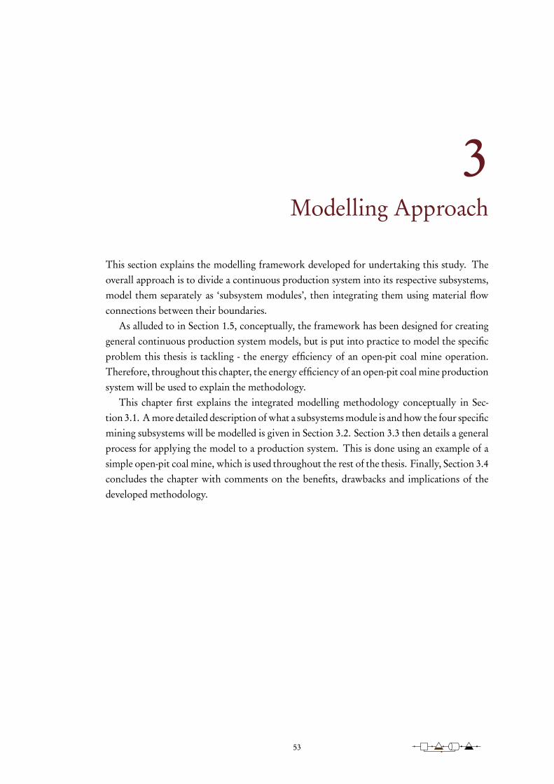
3Modelling Approach
This section explains the modelling framework developed for undertaking this study. Theoverall approach is to divide a continuous production system into its respective subsystems,model them separately as ‘subsystem modules’, then integrating them using material flowconnections between their boundaries.
As alluded to in Section 1.5, conceptually, the framework has been designed for creatinggeneral continuous production system models, but is put into practice to model the specificproblem this thesis is tackling - the energy efficiency of an open-pit coal mine operation.Therefore, throughout this chapter, the energy efficiency of an open-pit coal mine productionsystem will be used to explain the methodology.
This chapter first explains the integrated modelling methodology conceptually in Sec-tion 3.1. A more detailed description of what a subsystems module is and how the four specificmining subsystems will be modelled is given in Section 3.2. Section 3.3 then details a generalprocess for applying the model to a production system. This is done using an example of asimple open-pit coal mine, which is used throughout the rest of the thesis. Finally, Section 3.4concludes the chapter with comments on the benefits, drawbacks and implications of thedeveloped methodology.
53
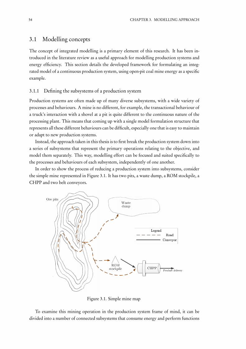
54 CHAPTER 3. MODELLING APPROACH
3.1 Modelling concepts
The concept of integrated modelling is a primary element of this research. It has been in-troduced in the literature review as a useful approach for modelling production systems andenergy efficiency. This section details the developed framework for formulating an integ-rated model of a continuous production system, using open-pit coal mine energy as a specificexample.
3.1.1 Defining the subsystems of a production system
Production systems are often made up of many diverse subsystems, with a wide variety ofprocesses and behaviours. A mine is no different, for example, the transactional behaviour ofa truck’s interaction with a shovel at a pit is quite different to the continuous nature of theprocessing plant. This means that coming up with a single model formulation structure thatrepresents all these different behaviours can be difficult, especially one that is easy to maintainor adapt to new production systems.
Instead, the approach taken in this thesis is to first break the production system down intoa series of subsystems that represent the primary operations relating to the objective, andmodel them separately. This way, modelling effort can be focused and suited specifically tothe processes and behaviours of each subsystem, independently of one another.
In order to show the process of reducing a production system into subsystems, considerthe simple mine represented in Figure 3.1. It has two pits, a waste dump, a ROM stockpile, aCHPP and two belt conveyors.
Figure 3.1. Simple mine map
To examine this mining operation in the production system frame of mind, it can bedivided into a number of connected subsystems that consume energy and perform functions

3.1 Modelling concepts 55
to achieve production targets of the whole mine. This breakdown can be seen in Figure 3.2,where borders are drawn around subsystems, and various material and energy flows are rep-resented by arrows.
Figure 3.2. Mine process flow diagram
From this subsystem breakdown, there are five subsystems connected to each other usingfour different material flows, ROM, product, waste and water. Each of the subsystems alsohas an energy consumption that can be summed up to represent the total energy consumptionof the system. For simplicity, the belt conveyor drawn in Figure 3.1 between the stockpileand processing plant is considered here as part of the stockpile reclaiming activity.
3.1.2 Subsystem concepts
The simple explanation of this study’s approach so far has explained that these subsystemscan now be modelled separately. However, upon further inspection, it can be seen that thesefive subsystems can be categorised as one of the four subsystems analysed in the literaturereview. There is one each of excavation and haulage, processing plant and belt conveyor andtwo stockpiles – thinking of the waste dump points as a stockpile. For larger, more complex,mines, the other subsystems may be replicated in the same way the stockpile has been here.This means, if the subsystem formulations are general enough, only four subsystems modulesshould need to be formulated. Their replications on site are then parameterised separately.
The most important prerequisite of a subsystem is that the connection points on its bound-aries, which connect it to other subsystems, are ‘material flow’ connections. A well-definedspecification of the boundaries of subsystems is required to properly allow for connectingthem together in any fashion necessary to represent a wide variety of mine layouts.
Using ‘material flow’ as the type of connection between subsystems is a key design featureof the modelling framework developed in this research. It has been decided upon under theconjecture that typical analysis and decision making for continuous production systems arebased around the flow of material. This is supported by literature reviewed in Section 2.5.
Ideally, a set of subsystem modules can be formulated generally enough to be used torepresent the vast majority of subsystems that are used in actual open-pit coal mines. The term

56 CHAPTER 3. MODELLING APPROACH
‘general’ is used here to indicate that the specifics of a subsystem’s operation are adaptablethrough parameters of the model rather than structural changes to the formulation. Forinstance, a general excavation and haulage subsystem formulation should be scalable, withinreason, to any number of pits, destinations, trucks, shovels that may arise at an operatingmine. More specifically, the operational detail of the trip times, loading times and energyconsumption should also be parameters that can be changed to suit the particular mine beingmodelled. Similarly, a stockpile should be modelled generally enough to be able to have anumber of different inlet and outlet connection points, store any material type and allow fordifferent limits on stacking, reclaiming and overall inventory, all through parameters.
With this set of general subsystems, a library of these generic models can be assembled.This means the effort of subsystem modelling can be performed once then reused across newmines being modelled. The idea behind this is to reduce the effort of applying the developedmethodology to a new mine, enabling any potential value to be realised sooner at a lower cost.It also means problem domain experts, such as mine operators, can modify the model of theiroperation using the appropriate parameters, without needing to change the mathematicalformulation.
More specific details about the concepts behind modelling subsystems, along with inform-ation about each particular subsystem module, are presented in Section 3.2.
3.1.3 Integrating the subsystems
Once the subsystems modules have been formulated, they are then integrated into singleformulation, the integrated model. This has been designed to be a simple process, withthe intention being that it can be performed by a domain expert, such as a mine manageror operator, as opposed to a mathematical modeller. This concept is explored further inSubsection 9.1.2. The basic process of creating the ‘top level’ model of the mine can besummarised by the following steps:
1. Select subsystems used on the mine
2. Connect subsystems to one another
3. Parameterise the subsystem operation
4. Combine their objectives in a function
The first two steps turn the mine into a structured process flow representation. Their pur-pose is to convert the mine’s physical operation into a logical representation of the subsystemsand their connections, a transformation represented by the changes between the physical mapin Figure 3.1 and the process flow diagram in Figure 3.2.
It is easy to imagine how the first two steps could be implemented into a flowsheeting-style,software application. Users could drag and drop subsystems from a library and connect themup to represent the process flow of the mine being modelled.
The third step in this process is to fit the selected subsystems to their actual operation. Thisinvolves setting various parameters on each subsystem based on data taken from the mine’s

3.1 Modelling concepts 57
current operation. Accurate parameterisation of subsystems is a key step to getting realisticand useful results from the model. Fitting the parameters to the latest available data meansthe model will best represent the actual operation of the mine, and therefore search the mostrealistic space for an optimal solution. A less accurate selection of data for parameterisation,such as old data or design information, will mean the models will poorly represent the actualoperation and find solutions that may be inferior for the current mine’s behaviour.
Ideally, these parameters should come from up-to-date data, collected on-site as often aspossible. This way, any changes to the behaviour of the subsystems can be accounted for inthe next run of the optimisation. For instance, if a particular truck has degraded in efficiency,then its energy consumption parameterisation should be updated as data becomes available,which will then impact upon the model’s decision to use that truck over other trucks.
The last step is to create an overall objective based on the objective values coming from thesubsystem formulations. For this study, energy consumption, measured in MWh, is used. Itis simply the sum of all subsystem energy consumptions. As introduced in Section 2.2, onlythe denominator, energy consumption, of energy efficiency is used as the objective of theoptimisation model since the planned production is an input to the model. It is also selectedto ensure linearity of the objective function. More information on how the objective value isselected and defined is given with the subsystem concepts in Section 3.2.
3.1.4 Capacity
The capacity of a production system is a function of its subsystems capacities, which are inturn functions of their respective asset capacities, a factor that impacts production systemenergy efficiency, as introduced in Section 2.3. This reflects how the modelling frameworkdeveloped here handles capacity. There is no explicit whole-of-system level modelling featurethat deals with capacity. The capacity of the whole system is implicitly described by theparticular subsystems that have been connected to create the integrated model, as explainedin the previous subsection.
As subsystems interact with each other through material flow connections, the capacitiesof subsystems must be modelled to constrain the material flow. This will mean connectedsubsystems will implicitly be constrained by one another and hence the whole system willhave an implicit capacity. Since subsystem formulations are distinct from each other andhave few requirements, the specifics of how the capacity constraints are implemented are leftcompletely up to the modeller. Once again, this freedom enables subsystem formulations tobest represent their actual operation.
By handling the capacity in this manner, integrated models created using this frameworkcan provide valuable insight into the production system’s actual capacity. Sensitivity andscenario analysis can be used to compare the current operation against the maximum capacityand identify where and when bottlenecks may be occurring. These are valuable for examiningmany types of production system performance measures, including energy efficiency.

58 CHAPTER 3. MODELLING APPROACH
3.1.5 Operating states
The literature review, in Section 2.3 and 2.4, mentioned the importance of modelling dif-ferent operating states of subsystems and equipment when optimising energy efficiency. Inparticular, it was identified as an area to help link the asset usage and planning factors whilemodelling. While it was well modelled amongst the processing plant, stockpile and beltconveyor models, it was identified as a deficiency with many of the excavation and haulagemodels. It is therefore an important and valuable concept to employ within the integratedmodelling framework.
In this framework, the time dimension of the optimisation is partitioned into multipleoperating states, as indices, that can have different lengths. An operating state, also referredto as a state, is defined as the period of time in which no changes to the overall work beingperformed by each and every subsystem occur. During which, the amount of material flowingbetween subsystems remains steady. The term operating state, or state, is used here overmore traditional operations research modelling terms such as time step or interval, as it moreaccurately describes the problem domain being modelled.
The variable length of states gives the model the ability to have increased resolution aroundtimes where more changes in operation may occur, and reduce resolution when stable oper-ation is occurring. While they are an input into the model and can’t change dynamicallywithin the optimisation, they can be programmatically determined before runtime based onthe input plan or other parameters.
This concept can also be used to help reduce the problem instance size to increase solutionspeed. Though, having varied state lengths instead of having smaller equally sized time stepsmay inhibit the optimisation from finding a more optimal solution, which is a question ofspeed versus accuracy with regards to the model formulation.
The concept of operating states can also help reach more realistic solutions for operatorsto comprehend and follow. For example, using small state lengths of 10 minutes, dependingon the detail and correctness of the subsystem models, the optimal solution may be to rampproduction of a particular subsystem up and down within the 10 minute states, which maybe feasible in the model, but result in unwanted behaviour in real life. Even if it is feasibleand optimal in real life, giving such tight instructions to operators may be too hard to follow.In a period where there are no changes to the overall operation of the mine, fewer sets of in-structions for that time period will likely be easier for an operator to follow, than a multitudeof instructions over small time steps. Measures can be taken when formulating the model toreduce this effect, though these extra measures will likely increase the size of the problem andslow down the solution.
It should also be noted that the length of states doesn’t necessarily mean subsystems can’timplement their own internal time dimension, so long as they aggregate the internal beha-viour up to boundary connection material flows for each state. This is performed later in thisthesis, in Chapter 6, to give more accuracy to the modelling of equipment operations withinthe excavation and haulage subsystem.

3.1 Modelling concepts 59
3.1.6 Solving
After the integrated model has been created, it now only needs one more piece of informationto be solved - the operating plan. This is considered the primary input of the optimisation.
Planning happens across various levels and time scales in mining. In general, as explainedin the literature review, long and medium-term plans are based on the NPV of the mineand decide on a required production rate to maximise the NPV. The shorter term plans arethen devised to meet these production targets with minimum cost. Short-term planning andscheduling can be done to various degrees on a mine. The short-term plan for the mine isused by managers and operators to determine the daily operation of the mine.
These plans are used to define the work required for the mine to complete over the op-timisation horizon. This research conceptualises a plan as a series of ‘tasks’ that the mine, asa system, must complete. These tasks have start and completion times, and can span acrossthe whole mine. For example, there may be a task to produce a certain amount of productbefore the end of the day; a task to extract an amount of overburden before halfway throughthe day; a task to extract the ROM coal after the overburden has been uncovered; or a task tohave a certain level of stockpile by a particular time.
The ability to add different types of tasks to different parts of the mine enables push orpull-based modelling. For example, a push-based task would be an extraction target, whereasa target on demand would represent a pull-based task.
Once these tasks are placed on the integrated mine model, it is ready to be optimised.This is where connection material flows are solved alongside subsystem specific decision vari-ables subject to achieve the defined tasks, satisfy constraints internal to each subsystem andminimise energy consumption.
Being able to optimise the collection of all decision variables, and satisfy all constraints, isthe key benefit to the integrated approach. Even though each subsystem has been modelledand parameterised separately to suit their particular functions and behaviour, they are now inthe same solution space for the optimiser to search for the global optimum across the wholemine, rather than each subsystem individually.
The subsystems are now implicitly constrained by each other and the overall productionand demand requirements of the whole mine system. Any change made by the optimiser toreduce energy consumption on one subsystem will only be selected if it does not increasethe energy consumption on another subsystem by a greater amount or violate any otherconstraints.
Using this model, decision support provided to the operators of each subsystem can be‘aware’ of that subsystem’s impact on the whole mine energy consumption, the main benefitbehind the concept of whole-of-system modelling. This leads to operational decisions thatimprove the whole mine’s energy efficiency, rather than simply each subsystem on its own,which can result in sub-optimality for the whole system.

60 CHAPTER 3. MODELLING APPROACH
3.2 Subsystem modelling concepts
This section details the requirements of subsystem modules to work in the proposed mod-elling framework. As previously discussed, since the various subsystems that make up acontinuous flow production system can be quite different in nature, there is no one math-ematical representation for a subsystem. Instead there are requirements for subsystem modelformulations to adhere to that allow them to be connected up and solved together.
The generic form of a subsystem module is represented below in Figure 3.3. It has materialflow inlet and outlet connections, energy consumption and is characterised by parameters thatdefine its specific behaviour based on actual operation. The operating state time dimensionmentioned in Subsection 3.1.5, not shown in Figure 3.3, is also a feature of the subsystem.Each operating state of the integrated model represents the amount of time that the materialflow over a subsystem boundary connection is maintained.
Figure 3.3. Generic subsystem modules
Subsystems can be modelled to various degrees of complexity to represent the functionsthey perform, depending on a range of different factors. Relatively simple processes, such asbelt conveyors, may only require basic linear programming models to meet the requirementsof the optimisation, whereas complicated processes, such as truck and shovel fleets, mayrequire much more complicated MILP formulations to provide valuable results to the mineoperator. Known problem areas in the production system, where bottlenecks occur, can alsobe focused on with detailed modelling to make sure they are realistic enough for accurateoptimisation. Limited data availability also affects the ability to model subsystems with detail.
The four subsystems modelled in this study are excavation and haulage, processing plant,stockpile and belt conveyor. Each of these haves been modelled using the concepts outlined inthis chapter. Knowledge, gained from the research, and experience, from the case study mineexamined in this thesis, have been used in order to create a fairly general set of subsystemmodules for reusability on new mines.
This section first details the specific requirements of subsystem models in Subsection 3.2.1,then outlines strategies to take and considerations to make when developing subsystem mod-els in Subsection 3.2.2. The remaining four subsections (3.2.3, 3.2.4, 3.2.5 and 3.2.6) outline

3.2 Subsystem modelling concepts 61
the modules of the four subsystems being studied in this thesis.
3.2.1 Subsystem model requirements
As explained previously, there are basic requirements of subsystems, in order for them to beconnected to each other and used in the integrated modelling framework. These requirementsare as follows:
1. That material flow connection points exist on boundaries
2. That they are responsible for constraining the material passing through their connec-tion points
3. That they contain a variable representing the subsystems energy consumption
The first of these requirements ensures all subsystems can be connected to one anotherin any matter, to allow for representing any configuration of an open-pit coal mine. Thereare a number of different types of materials that are transported throughout a productionsystem, and the general concept of a connection allows for any number of materials to betransported over it. The main constraint of this requirement is that the connection pointrepresents a ‘flow’ of the arbitrary material being transported; in terms of modelling, thismeans it is a continuous variable with a ‘per time’ unit, such as tonnes/hour or litres/minute.Specifically, hours are being used as the time unit (denominator), as this is what is typicallyused in the mining industry. The numerator of the flow unit is dependent on the materialbeing transported. For example, tonnes are used for measuring the ROM and product coal,while kilolitres are used for water. The only necessity for the numerator is that each differenttype of material uses the same unit across the subsystems, not that all materials use the sameunit.
This first requirement has the most implications on the design of the framework outlinedin this research. It is principally an assumption of both the top level integrated model and theinteractions between subsystems. While it allows any subsystem to be trivially connected toany other subsystem at the top level, it assumes that this connection is appropriately repres-ented by a flow of material. The flow connection has been used based on the research intohow open-pit coal mines operate as continuous flow production systems, and from industryexperience in seeing production rates used at this level of mine management and operation.
In general, there is no restriction on the number of inlet and outlet connection pointsa subsystem can have. It may be that a specific subsystem has physical limitations on thenumber of inlets or outlets it has, however that is considered an implementation detail ofthat specific subsystem model, rather than a limitation of the general subsystem buildingblock definition.
The second requirement asserts that each subsystem model must include any constraintson the material passing in and out through its connection points are defined internally, asintroduced in Subsection 3.1.4. This allows for a connection at the top level to be a completelygeneric concept, so technically any two subsystems can be connected to one another at the

62 CHAPTER 3. MODELLING APPROACH
top level, but their respective internal model will dictate whether there is any valid materialand how much of it can flow between them. This increases the amount of flexibility there isfor creating the integrated top level models for specific mine setups.
To explain how this works for constraining the type of material that flows through asubsystem, consider a truck and shovel fleet that transports top soil, overburden and ROMcoal and delivers to three different locations: a top soil dump, overburden dump and the ROMstockpile. To keep the model general, the truck and shovel subsystem should not need to beexplicitly aware of the type of material it is delivering to each outlet; however, the destinationsubsystems will be set up with constraints to only receive the type of material they can handle.So once they are connected and being solved in the same model, there will be the implicitconstraint on the truck and shovel fleet to only deliver the appropriate material to each of itsoutlets.
As well as this, the requirement means the capacity of subsystems should constrain theamount of material that can flow in and out of the subsystem to implicitly constrain anyconnected subsystems. For instance a belt conveyor may have a capacity of 3000t/h but if it isconnected to a processing plant that can only take in 2000t/h, it will be implicitly constrainedby the processing plant’s capacity.
The final requirement is there for use when integrating the models at the top level. Sinceminimising energy consumption is the objective of the optimisation, each subsystem is as-sumed to have a common variable for its own energy consumption to be summed up togetherat the top level in the objective function. The energy unit megawatt hour (MWh) is used asthe unit for this variable across all subsystems. This means certain energy sources, such asdiesel, must be converted into their energy value, rather than the measured volume or mass,which may be used internally in the subsystem.
The modelling framework is by no means limited to the energy efficiency problem andcould easily be suited to alternate problems with other decision variables. For instance, thesubsystem module formulations could use greenhouse gas emissions as their objective valuesto optimise the environmental impact of a mine’s operation. It is, however, important tokeep all subsystems using the same unit so the addition of their individual values makessense. A multivariable cost function that assigns dollar values to several different componentsof a subsystem’s operation, such as labour, parts and energy costs, is one way of includingmore than one component in the optimisation. Other multi-component objective functions,coupled with appropriate solution techniques, could also work within the framework, thoughare not considered in this study.
With these three requirements satisfied, a subsystem model is ready to be included into theintegrated model. Not that it would be particularly useful with just these three requirementssatisfied; the intention of this design is to allow for the basic subsystem’s building blockto be as simple as possible. Then from that building block, the complexity comes fromthe mathematical modelling, which is done specific to the functions and behaviour of thesubsystem. This concept is designed to avoid the effort of trying to fit the functions andbehaviours of a new subsystem into an existing, tightly constrained modelling structure.
3.2 Subsystem modelling concepts 63
3.2.2 Subsystem modelling strategies
Modelling the subsystems can be carried out with various degrees of sophistication. Thisdepends on both the production system being modelled and the desired performance of theoptimisation.
A primary factor in deciding on the complexity of the model, as with most optimisationmodel efforts, is the balance between solution speed and accuracy. In order to model the exactoperation of a mine with all of the equipment being used, a very large number of variablesand constraints would be required, making solving the model in reasonable time unviable.Instead, assumptions must be made and model detail lessened in order to reduce the size ofthe problem.
The detail of the model may also be limited by the availability of data for the particularsubsystem at the mine. In the case study used in this research, there is limited data aboutwhere exactly the energy is consumed in the processing plant. This limits the ability toproperly model the inner workings of the plant, whereas, with more data, a more detailedrepresentation of its control, equipment and energy consumption could be formulated.
Another factor in deciding how much effort to place on modelling a particular subsystem,is whether it is, or may become, a bottleneck of the whole system. As stated in the literaturereview, bottlenecks have a major impact on energy efficiency. Making sure there are goodrepresentations of possible bottleneck subsystems will allow for the integrated model to takeinto consideration the increased impact that operation of that subsystem has on the rest ofthe production system.
In this early stage of the research, another factor in the development of subsystem models isthe reusability. Keeping assumptions fairly general and creating relatively simplistic models ofthe subsystems means that they can form a library of reusable subsystem models which, whilenot perfectly, should apply to most mine setups. With general models like this in a library, itcan be relatively quick to parameterise them and connect them up into the integrated modelto get something going.
In order to get a better representation of the specific system being modelled, it may then beappropriate to take one of the standard library subsystem models and alter it to suit particularintricacies of the mine. This follows a more ‘agile’ style of model development, wherebya running optimisation is always available, with extra effort placed on improving it whenrequired (if at all). This is opposed to the more traditional approach of a large upfront mod-elling effort across the whole mine. This ‘agile’ approach of modifying existing subsystemsfor accuracy improvement is applied in Section 6.1.
The subsystems developed in the following sections take into consideration all of thesefactors. The case study mine is used as the reference point for data availability, bottlenecksand how general the models can be while still representing the operation well enough to geta quality solution.
In order to develop subsystem models, a number of different resources can be drawnupon. Research papers provide a good source of mathematical models for the various sub-systems that are modelled. Even if they do not deal with energy explicitly, the variables

64 CHAPTER 3. MODELLING APPROACH
and constraints for defining the operation will likely be easily extended to relate to energyconsumption.
Industry may also have proprietary optimisation models that could be useful for definingthe subsystem modules if access to them is permitted. For instance, CHPPs may have op-timisers built into their automated control systems; this could serve as the beginnings of themodel developed for this framework.
Another way to build models would be to create extremely general mathematical modelsthat can be empirically fit to operation data, to represent a wide variety of processes.
In general, most formulations for the subsystems will contain some level of empiricallyderived parameters. For instance, diesel consumption of each truck can come from opera-tional data on the consumption of each truck. Using this type of information in the model,as opposed to design data, is important for getting an accurate representation of the operationof the mine. This means the solution will be the best for the actual operation of the mine,rather than its theoretical operation. Keeping this data up to date is important in making surethe solution stays relevant to the actual operation.
A suggestion for formulating general subsystems is to not use operating states’ time indicesin parameters, unless the modeller is certain that the states won’t change across differentinstances or that it is completely unavoidable. Since states are designed to come in varyingquantity and length, having a parameter that is indexed by state would mean it may have tobe updated every time the state length changes.
3.2.3 Excavation and haulage subsystem
The excavation and haulage subsystem developed for this research determines the activityof the trucks and shovels that are working together to dig raw material from the ground anddeliver it to its required destination. Due to the complex nature of the excavation and haulageoperation, it will require the most sophisticated model of the four subsystems studied in thisresearch. Figure 3.4 outlines the key elements of the excavation and haulage subsystem thatwill be modelled in Section 4.1. Inlet and outlet connections are also labelled with examplesof what the subsystem may be connected to.
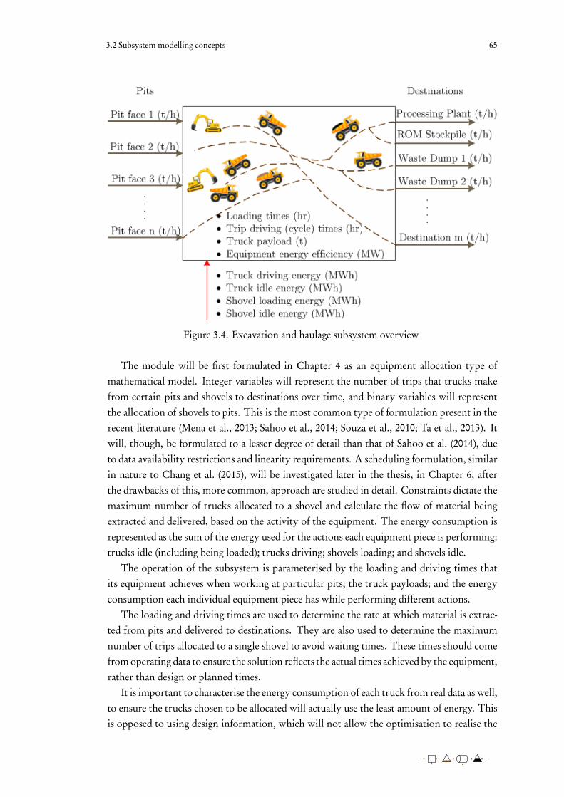
3.2 Subsystem modelling concepts 65
Figure 3.4. Excavation and haulage subsystem overview
The module will be first formulated in Chapter 4 as an equipment allocation type ofmathematical model. Integer variables will represent the number of trips that trucks makefrom certain pits and shovels to destinations over time, and binary variables will representthe allocation of shovels to pits. This is the most common type of formulation present in therecent literature (Mena et al., 2013; Sahoo et al., 2014; Souza et al., 2010; Ta et al., 2013). Itwill, though, be formulated to a lesser degree of detail than that of Sahoo et al. (2014), dueto data availability restrictions and linearity requirements. A scheduling formulation, similarin nature to Chang et al. (2015), will be investigated later in the thesis, in Chapter 6, afterthe drawbacks of this, more common, approach are studied in detail. Constraints dictate themaximum number of trucks allocated to a shovel and calculate the flow of material beingextracted and delivered, based on the activity of the equipment. The energy consumption isrepresented as the sum of the energy used for the actions each equipment piece is performing:trucks idle (including being loaded); trucks driving; shovels loading; and shovels idle.
The operation of the subsystem is parameterised by the loading and driving times thatits equipment achieves when working at particular pits; the truck payloads; and the energyconsumption each individual equipment piece has while performing different actions.
The loading and driving times are used to determine the rate at which material is extrac-ted from pits and delivered to destinations. They are also used to determine the maximumnumber of trips allocated to a single shovel to avoid waiting times. These times should comefrom operating data to ensure the solution reflects the actual times achieved by the equipment,rather than design or planned times.
It is important to characterise the energy consumption of each truck from real data as well,to ensure the trucks chosen to be allocated will actually use the least amount of energy. Thisis opposed to using design information, which will not allow the optimisation to realise the

66 CHAPTER 3. MODELLING APPROACH
difference between trucks and therefore will not necessarily result in a real life optimum. Thiscan also improve the performance of the optimisation, as it reduces the amount of symmetryin the solution space.
3.2.4 Processing plant subsystem
A fairly general model of the processing plant will be developed, similar to that of Middelberget al. (2009) but still using the same overall, inlet and outlet federate, decision variables at thecore of more advanced models (Matthews & Craig, 2013; Numbi & Xia, 2015). This is due tolimited data availability for the processing stages in the case study of this thesis as well as toalign with the objective of creating a general model to allow for reusability on other mines.Figure 3.5 gives an overview of the processing plant subsystem module, with example inletsand outlets, presented formally in Section 4.1.
Figure 3.5. Processing plant subsystem overview
The model assumes known ratios for inlet ROM material grades and water to outletproduct grades and waste material. It is also constrained by maximum inlet and outletcapacities. The energy consumed by the plant is assumed to be proportional to the grade andamount of ROM it is processing and the grade of product it is producing.
All of these parameters should be able to be fit from real operational data in order to getthe best picture of the actual behaviour of the plant. Without detailed data or a detailed modelof the subsystem, it is important to get what is available as accurate and up-to-date as possibleto allow for the solutions to be close to reality.

3.2 Subsystem modelling concepts 67
3.2.5 Stockpile subsystem
The proposed stockpile model will also been developed to be as generic as possible, so it canapply to many different stockpiles with limited data availability. A network flow model withinventory is used as the basis for the formulation, similar to Ta et al. (2005) and Hanoun et al.(2013). The key elements of the stockpile subsystem module, formulated in Section 4.1, areshown in Figure 3.6 with example connections into and out of the subsystem.
Figure 3.6. Stockpile subsystem overview
Maximum flow rates for stacking and reclaiming are used, along with a minimum stockpilelevel for each grade being stored. Energy usage is assumed to be proportional to the flowrates of material being stacked and reclaimed from the piles; this is characterised based on thespecific equipment used to stack and reclaim for each particular stockpile being modelled.
As with the other subsystems, it is just as important to get accurate and up-to-date opera-tional data for parameters to be able to realise maximum value from the model.
3.2.6 Belt conveyor subsystem
Belt conveyors will also formulated as simple network flow models, but without inventory,in a similar fashion to Middelberg et al. (2009). This is done, as with other subsystems, to beas general as possible to suit a wide variety of belt conveyors and data availability. Figure 3.7outlines the key elements, with example inlet and outlet connections, of the belt conveyorsubsystem formulation that is presented in Section 4.1.
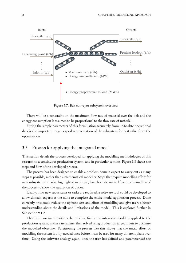
68 CHAPTER 3. MODELLING APPROACH
Figure 3.7. Belt conveyor subsystem overview
There will be a constraint on the maximum flow rate of material over the belt and theenergy consumption is assumed to be proportional to the flow rate of material.
Fitting the simple parameters of this formulation accurately from up-to-date operationaldata is also important to get a good representation of the subsystem for best value from theoptimisation.
3.3 Process for applying the integrated model
This section details the process developed for applying the modelling methodologies of thisresearch to a continuous production system, and in particular, a mine. Figure 3.8 shows thesteps and flow of the developed process.
The process has been designed to enable a problem domain expert to carry out as manysteps as possible, rather than a mathematical modeller. Steps that require modelling effort fornew subsystems or tasks, highlighted in purple, have been decoupled from the main flow ofthe process to show the separation of duties.
Ideally, if no new subsystems or tasks are required, a software tool could be developed toallow domain experts at the mine to complete the entire model application process. Donecorrectly, this could reduce the upfront cost and effort of modelling and give users a betterunderstanding about the details and limitations of the model. This is explored further inSubsection 9.1.2.
There are two main parts to the process; firstly the integrated model is applied to theproduction system, in this case a mine, then solved using production target inputs to optimisethe modelled objective. Partitioning the process like this shows that the initial effort ofmodelling the system is only needed once before it can be used for many different plans overtime. Using the software analogy again, once the user has defined and parameterised the

3.3 Process for applying the integrated model 69
subsystems in the integrated model, the model would be ‘saved’ as a completed model, then‘loaded’ and given a plan to optimise each time it is required.
The remainder of this section steps through the process using a basic hypothetical mine asan example. This example is then used for validation in Chapters 4, 6 and 7. Chapter 5 usesthis process to apply the model to an open-pit coal mine in South East Queensland as a casestudy.
Figure 3.8. Process for applying the integrated model
3.3.1 Gather production system information
The first step of the process is to gather information about the operation of the productionsystem being modelled. Information can come from a number of sources, such as discussionwith managers, operators or other employees; operational data; long, medium and short-term plans; maps; and existing models. The work required to carry out this step can varydepending on several factors, such as the modeller’s knowledge / experience, availability ofdata and the complexity of the production system.
Completing this step can be a little open-ended as there are typically a lot of observationsto make across a production system to learn its operation, and a mine is no exception. Theaim of the step is to get enough of an understanding of the system to help with completingthe rest of the process. It is therefore important to focus the effort of making observations towhere it will be useful. In reality, this step should be revisited throughout the whole processto make sure the mine model being developed is as good a representation of the system as

70 CHAPTER 3. MODELLING APPROACH
possible.In order to provide some rigour around this step, a series of questions have been compiled
to help the modeller form useful observations for the later stages of the process. Thesequestions have been created specifically for the mining case studied in this thesis, though theydo give an indication of the types of questions that should be being asked of a different typeof production system being modelled. They are also by no means exhaustive. The questionsare outlined below and answered for a simple hypothetical open-pit coal mine. They arebroken up into six parts; the first relates to the mine as a whole, the following four relate tothe subsystems that make up the mine and the final one is used to capture knowledge aboutsubsystems that are at the mine but not considered in this research.
The questions are principally about getting the information that is required to create thecorrect model structure at the whole-system and subsystem level. That is, they focus onfinding out what is important and relatively static within the mine and leave the more specificdetail for later in the process when each subsystem is parameterised. For instance, the numberof shovels is not likely to change often and is important information as it used to define the sizeof the mathematical formulation, so it is absolutely necessary to solve the model. However,each shovel’s idle and loading energy usage is left for the later parameterisation stage. This isbecause it is likely to change over time as the shovel’s efficiency changes, when it degrades orreceives maintenance, and can also be estimated based on design data or by other means tosolve the model before it is parameterised from real data.
Whole-of-mine questions
These questions help contextualise the mine in a continuous production system setting todefine the problem and break it up into a series of connected subsystems.
What are the boundaries of the mine?A good way to answer this question is to draw a rough map of the mine to see the physical
flow of material through the mine, from start to finish. Figure 3.9 shows a rough map of thesimple mine being used in this section. In this case, the material is being extracted from onepit face, and either ends up at a common waste dump or delivered via belt conveyor.

3.3 Process for applying the integrated model 71
Figure 3.9. Simple hypothetical mine map
In a real life scenario, defining the boundaries may depend on limitations of the respons-ibility the organisation doing the modelling has. For instance, if a contract miner is onlycontracted to deliver ROM to a stockpile, the end boundary of their modelling effort may bethat stockpile, or even just before it. Alternatively, in a case where two pits are operated bythe same organisation and feed the same CHPP and product delivery, then both pits and thedelivery loader should be defined as the boundaries.
What systems perform the majority of the work?Once the boundaries have been defined, the modeller should now look within them to
observe what work is being performed to transport and process the materials from the be-ginning to end boundaries. In this example, we can see that there is excavation and haulage,ROM stockpile, waste dump, CHPP and three belt conveyors. These systems work togetherto extract the material out of the ground to be transported, processed and delivered.
What are the main energy consumers of the mine?This question aims to compliment the last and make sure there is no major energy con-
sumption that will be overlooked. The model should aim to include both the main operationand material flow of the mine and the main energy consumption. Typically, and in the caseof this example mine, these two go hand in hand; the same systems that contribute to theprimary operation of the mine will also be the biggest energy consumers. However, theremay be cases where an auxiliary system consumes a large amount of energy, without havingmuch to do with main flow of material and therefore should at least be considered at thispoint, then evaluated in a later stage as to how it may fit into the model and what value canbe achieved at an operational decision making level.
How many different types material are transported between systems?This question determines what grades of raw ore, waste, product and other materials are

72 CHAPTER 3. MODELLING APPROACH
being transported and used across the mine. A good starting point to answering this questionis to think about what material is transported between the systems that make up the mine, aswell as any other material that is consumed, such as water. For the example mine here, thereare five types of materials, the ROM coal extracted from the ground; waste in the form ofoverburden and tailings; product coal output from the CHPP; and water used by the CHPP.
Excavation and haulage questions
These questions should be answered as many excavation and haulage subsystems have beenidentified in the previous set of questions related to the mine as a whole. They are used todetermine the main attributes of the subsystem and its boundaries. The specific operationalcharacteristics are determined and defined in the later, subsystem parameterisation phase ofthe process.
What are the boundaries of the subsystem?The answer to this question is used to work out how many inlets and outlets the excavation
and haulage subsystem has. The inlets are the pits / faces being extracted from, the outletsare the destinations to which the trucks deliver.
There are two pits being extracted from in this simple example, and three destinations, theROM stockpile, CHPP and waste dump.
What grades are being extracted?This is for working out what material grades are extracted by the fleet. It is particularly
important in certain cases. For instance if there are two fleets, one for coal and one for over-burden, it is important to distinguish what material each fleet is extracting. In this example,the shovels can dig either ROM coal or overburden material from the pit.
How many shovels are there?This is a straightforward question for defining the number of loaders that the model will
have available for parameterisation in later stages. In the simple hypothetical example, thereare two shovels.
How many trucks are there?In a similar fashion to the previous question, this question is for defining the right amount
of trucks in the model for the later parameterisation. For this example, there is a fleet of sixtrucks.
Processing plant questions
Along with the excavation and haulage questions, these are used to gather the general in-formation about the processing plant subsystems at the mine, which enables them to beparameterised in more detail in a later stage of the process.
What are the boundaries of the subsystem?The processing plant can receive ROM coal from a number of different locations, and
typically will also have an inlet of water. The outlet boundaries of the processing plant willusually consist of at least one for product and one for tailings waste, but depending on the

3.3 Process for applying the integrated model 73
complexity of the plant and mine, there could be multiple product and tailings outlets. Inthis example, there are two ROM inlets, a water inlet, product outlet and a waste outlet.
What materials can be processed?This is used to define what types of raw material are accepted by the processing plant for
transforming into product. In this example, it is the ROM coal material grade that is processedby the CHPP.
What materials are produced?This question is used to define what product grades are yielded by the processing plant
as outputs. The product coal material grade is the answer to this question for this workedexample.
Stockpile questions
The questions to answer, relating to the stockpiles, are similar to the other two subsystems.They are focused on defining the basic operating behaviour of the mine, allowing the subsys-tems to be parameterised in more detail later in the process.
What are the boundaries of the subsystem?Much like the other subsystems, this question is used to define the inlets and outlets of the
stockpile. In this example, there are two stockpile subsystems. The ROM stockpile has oneinlet and one outlet, while the waste dump has one inlet and no outlet.
What grades are stored in the stockpile?This is used to define the grades allowed in and out of the subsystem and also the number
of stockpiles in the subsystem. The ROM coal grade in this example is the grade stored bythe ROM stockpile, and the waste dump can only accept and store overburden.
Belt conveyor questions
Once again, the questions related to this subsystem are made to simply define the primaryoperation of the subsystem so it can be parameterised specifically in a later stage of the process.
What are the boundaries of the subsystem?As with the other subsystems, this question is used to define the inlets and outlets of the
subsystem. Belt conveyors are modelled to have a complete mass balance over them, so musthave at least one inlet and outlet. The belt conveyor in this example has a single inlet and asingle outlet.
What grades can be transported over the belt conveyor?Depending on the type of belt conveyor, it may be that any grade can be transported over
it, but in general it is a good idea to define what the belt conveyor is used for specifically tomake sure it is not hooked up incorrectly when it is connected to the upstream and down-stream subsystems. In this example the belt conveyor transports product coal.
Other subsystem questions
This final section of questions is for any of the subsystems that have been identified by thewhole-of-mine observations but cannot be related back to one of the four general subsystems

74 CHAPTER 3. MODELLING APPROACH
defined in this research. Depending on their importance, they may or may not need tobe developed as new subsystems at a later stage of the process. These questions will helpdetermine whether that effort is actually required, and to help with the modelling if it is. Inthe simple example being explored here, and ideally, these questions would not be required,so there will only be a description of each question.
What are the boundaries of the subsystem?Once again, they are used to work out how many inlet and outlet connections the subsys-
tem has.What materials does the subsystem work with?This is important to help get an idea of what type of function the subsystem is per-
forming, whether there is any transformation of material happening, or if it performstransport/handling type work.
How is energy consumed on the subsystem?This question is important in determining how to model the subsystem to ensure it con-
tributes to the objective function; it can also be used as evidence to show that modelling maynot be necessary if there is very little energy consumed by the subsystem.
What decisions are made to determine the operation of the subsystem?In order to determine the structure of the mathematical model to be developed for the new
subsystem, answering this question will help scope the required resolution of the decisionvariables. They may only be the overall flow through the subsystem, or may have to relate toequipment allocation or stock levels.
How do operational decisions on this subsystem impact energy consumption?This is to help get an idea about what parts of the model impact energy consumption to
make sure everything is included in the total energy consumption of the subsystem.How do operational decisions on this subsystem impact other subsystems?This question works to both ensure creating the new model is worth it from the perspect-
ive of the main operation of the mine, and secondly, to assist in ensuring it will constrain thewhole system in a realistic nature.
3.3.2 Outline process flow of system
This step in the process formalises some of the observations made in the first step, aboutwhole-system boundaries and subsystems. This is done by representing the mine as a series ofconnected subsystems on a Process Flow Diagram (PFD). This has been done to the examplemine being used in Figure 3.10.

3.3 Process for applying the integrated model 75
Figure 3.10. Simple mine process flow diagram
The process flow diagram should contain all of the subsystems that were identified asbeing part of the main flow of material through the mine and/or large contributors to energyconsumption.
The sub-step involved in completing this process flow diagram, as seen in Figure 3.8, is toalign the subsystems with the standard set, or library, of subsystem models. This researchcontains four standard subsystem models. As per the next block in the process after this, ifthere is a subsystem that cannot be represented by one of these four standard models, anddepending on its importance and the effort required to model it, a new subsystem may berequired to be mathematically modelled before the process can be continued. This is explainedin Subsection 3.3.3.
As introduced in previous sections, thinking of this step in a software sense, it is easy toimagine how it could be adapted to a flowsheeting type tool, where the library of standardsubsystems can be ‘dragged and dropped’ onto a canvas and connected up to one another. ThePFD created both visually and logically could then be processed by the software to make astart on defining the model in the mathematical modelling language.
3.3.3 Formulate new subsystem model(s) (if required)
As introduced in Subsection 3.3.2, the decision block that asks if any new subsystems arerequired will determine whether any mathematical modelling will be required for applyingthis research to the mine. Ideally, for a minimum cost application the answer to this is no.This is the case for the simple example worked through in this section and the case studypresented in Chapter 5. However, a description of how to create a new subsystem model willbe presented here.
Firstly, the subsystem should be analysed with respect to how necessary a new moduleof its operation is. Much of this can come from the general observations from the first stepof the process, and should be weighed up against the effort required to formulate the newmodule.
If there are very few operational decisions that impact the subsystem, its energy usage orother subsystems, then it may not be worth including them in the model, as there will be

76 CHAPTER 3. MODELLING APPROACH
limited operational decision support that the optimisation can provide.It may be that this process is able to be postponed for later as well. For instance, if the
subsystem can be overlooked without impacting much on the other subsystems, a model ofthe mine could first be created without the new subsystem and value can be realised withoutthe effort of modelling at this stage. The modelling effort can be postponed and re-evaluatedin more detail later, without slowing down the upfront effort of getting the initial model upand running.
If it is absolutely critical to have the new subsystem modelled, it may be possible to takea low cost approach to modelling the new subsystem. Creating a very simple mathematicalmodel to represent the subsystem as a black box with basic mass balance constraints andenergy consumption related to throughput may be all that is required to continue with theprocess. Then once it is running, a more detailed study can be conducted into whether furthermodelling will yield enough value to justify the effort or not.
It may also happen that one of these new subsystems is close to an existing one but does notquite fit the existing model. In this case, the modelling effort may be reduced by duplicatingthe closest existing subsystem and customising it to suit the new one.
The concepts and requirements described in Section 3.2 are used to define a new subsystemin this part of the process. The standard MILP techniques and modelling procedures can beused to create the parameters, decision variables and constraints, so long as there are boundaryconnections with material flows and there is a variable for energy consumption for use by theobjective function.
After this step is completed for all new subsystems that are deemed to be required at thisstage, the process can move onto creating an instance of the integrated model of the mine.
3.3.4 Apply structural information to integrated model
This step is fairly straightforward so long as the process flow diagram aligns with the libraryof subsystems, plus any new subsystems, and reasonable effort has been carried out in theobservation phase. Each subsystem can be added to its relevant set of that subsystem type,connected to the appropriate neighbouring subsystems and configured with the relevant extrainformation gathered during observations. Details about these are given in the full modelformulation presented in Section 4.1.
Going back to the explanation of how this would work in a software tool setting, thisstage could possibly be included as part of the process flow diagram creation stage if it isdesigned well enough to take in the more detailed information about each subsystem, suchas the number of shovels of an excavation and haulage subsystem, or the stored grades of astockpile. A flowsheeting tool that is aware of each subsystem to this degree would be ableto create a logical representation of the model with enough detail to be translated into themathematical modelling language with no user effort.

3.3 Process for applying the integrated model 77
3.3.5 Enter subsystem parameter values
Once the previous step of defining the structure of the integrated model has been conducted,the model should have enough information to have all of the decision variables defined. Thenext step required to be completed before it can be run is to parameterise the subsystems toallow for their constraints to become active, along with their respective energy consumptionvariables for use in the objective function. This will leave the integrated model to only requirethe planned tasks, for it to be defined completely and be ready to be solved.
Each type of subsystem needs different information as part of this step. Their requiredparameters will be described one by one below, followed by a general explanation about wherethis data can come from and what impact it can have on the ability of the model to providevaluable results.
Excavation and haulage parameterisation
In plain English, the parameters required for the truck and shovel operation are as follows,along with the values used for the simple example. These parameters are formally defined inSubsection 4.1.2 of the full integrated model formulation.
• Trip driving time – for each trip – See Table 3.1
• Loading time – for each pit – 3 minutes
• Payload (t) of each truck – See Table 3.2
• Energy consumption rate (MW) of each truck when driving between a pit and destin-ation – See Table 3.2, for this example the energy consumption rate is considered thesame between any pit and destination
• Energy consumption rate (MW) of each truck when idle – See Table 3.2
• Energy consumption rate (MW) of each shovel when loading – See Table 3.3
• Energy consumption rate (MW) of each shovel when idle – See Table 3.3
Table 3.1. Simple example trip driving times (minutes)
From row Inlets Outlets Base
to column Pit 1 Pit 2Processing
plantROM
StockpileWastedump
Base
Inlets Pit 1 - - 7 8 10 7Pit 2 - - 7 8 10 7
OutletsProcessing
plant5 5 - - - -
ROMstockpile
6 6 - - - -
Wastedump
7 7 - - - -
Base 5 5 - - - -

78 CHAPTER 3. MODELLING APPROACH
Table 3.2. Simple example truck parameters
TruckPayload(tonnes)
Idle dieselconsumption
(MW)
Driving dieselconsumption
(MW)1 250 0.34 1.702 250 0.32 1.653 220 0.37 1.904 220 0.30 1.555 220 0.33 1.756 220 0.34 1.40
Table 3.3. Simple example shovel parameters
ShovelLoading energy
usage (MW)Idle energy usage
(MW)1 3.10 0.652 3.20 0.60
Processing plant parameterisation
The following parameters, formally described in Subsection 4.1.2, are used to describe theprocessing plant subsystem’s operation, with the simple example values listed in Table 3.4and Table 3.5.
• Ratio of each input material required to produce each product material (t/t)
• Maximum capacity of plant (t/h)
• Minimum capacity of plant when in operation (t/h)
• Fixed energy consumption (of having plant in operation) (MW)
• Variable energy consumption coefficient (related to load of plant) (MW/(t/h))
• Energy due to change in load between operating states (MWh/(t/h))
Table 3.4. Simple example processing plant input ratios
Produced grade ROM Product Waste Tailings WaterProcessing
plantProduct coal 1.223 0 0 0 0.069148

3.3 Process for applying the integrated model 79
Table 3.5. Simple example processing plant parameters
Maximumcapacity of
plant
Minimumcapacity of
plant
Fixed energyconsumption
(MW)
Variable energyconsumption
coefficient(MW/(t/h))
Energyconsumption
from change inload
(MWh/(t/h))Processing
plant500 3,500 1.5 0.0023225 0.0023225
Stockpile parameterisation
To parameterise the stockpile subsystem’s operation, the following values are required.Table 3.6 provides the values used in the simple example and Subsection 4.1.2 presents themformally.
• Maximum rate of stacking (t/h)
• Maximum rate of reclaiming (t/h)
• Minimum level of each stockpile (t)
• Current/initial level of each stockpile (t)
• Stacking energy consumption coefficient (MW/(t/h))
• Reclaiming energy consumption coefficient (MW/(t/h))
Table 3.6. Simple example stockpile parameters
Storedgrade
Max. rateof
stacking(t/h)
Max. rateof re-
claiming(t/h)
Min. levelof pile (t)
Currentlevel ofpile (t)
Stackingenergy
consumptioncoefficient
(MW/(t/h))
Reclaimingenergy
consumptioncoefficient
(MW/(t/h))ROM
stockpile ROM 5,000 5,000 20,000 22,000 0.00066 0.00014666
Waste dump Ovrbdn 5,000 5,000 0 0 0.00066 0.00014666
Belt conveyor parameterisation
The parameters required to describe the belt conveyor subsystem operation are as follows,along with their values for the simple example in Table 3.7. They are mathematically de-scribed in Subsection 4.1.2 of the model formulation.
• Maximum rate of material flowing over belt (t/h)
• Energy consumption coefficient (related to load) (MW/(t/h))

80 CHAPTER 3. MODELLING APPROACH
Table 3.7. Simple example belt conveyor parameters
Maximum rate ofmaterial flowingover belt (t/h)
Energyconsumption
coefficient(MW/(t/h))
Belt conveyor 5,000 0.000146
General parameter considerations
Section 3.1.3 introduces some of the considerations which should be made when findingvalues for these parameters with regards to the ability for the optimisation to provide valuableresults. The idea is that the more up-to-date and accurate these parameters are, the more themodel will realistically represent the actual mine operation and therefore will be able to besolved to more realistic optimal solutions.
The ability to get accurate values for each of these parameters will depend on a number offactors. These include how well the modules represent the operation of the specific subsys-tem, the level detail of data being collected for each subsystem and how easy it is to use thisdata to update the parameters.
If there is sufficient data available and easily available across the subsystems, then theseparameters should be updated on the model as often as the data is collected to maintain themost up-to-date picture of the mine’s operation. Ideally, this could happen as an automatedstep by some sort of software application, which collects, processes and sets the parametersautomatically.
Realistically, to get through this stage and move on through the process, the paramet-erisation could occur using very limited amount of data, be it through design information,educated estimates or even sensible default values. This level of data will not provide max-imum value back to the user, however could be used as a stepping stone to move on throughthe process to get at least some value from the model before this step can be revisited at a laterstage and completed in more detail.
Once this step has been undertaken, the process has completed the first of the two mainphases, where, in the software analogy, it can be ‘saved’ out at a point ready for the next phasewhere the input (current plan) is entered, creating a concrete problem instance to be solved.
3.3.6 Enter shift production targets and define operating states
The remaining steps fall under the second of the two main phases of the process. This phase iswhere an existing plan for the mine’s operation is defined and entered into the model and themodel is solved to optimise the total energy consumption while completing the plan. Thisstep is about converting a plan into a form that can be used by the mathematical model.
Subsection 3.1.6 describes some of the concepts formulated for how plans are representedin the model by breaking them up into a series of ‘tasks’ that become constraints on the model.At the moment, there is only one type of ‘task’ allowed for in the model. This is the basic

3.3 Process for applying the integrated model 81
task, explained in Subsection 3.1.6 and formulated in Section 4.1, to transport an amount ofa particular material grade over a connection within a defined start time and stop time.
If there is an activity in the plan that cannot be represented using this type of task, thena new task type will need to be formulated mathematically and added to the model. Withinthe developed process, this is handled in a similar fashion to the steps that go back to themodelling domain and add new subsystems in.
The other part of this step is to define the length of operating states to optimise for. Asexplained in Subsection 3.1.5, the time dimension for the optimisation model is defined bythe number and lengths of operating states that are appropriate for the problem being solved.This is directly related to the shift being optimised and the tasks that represent the shift plan.For a mine operating under normal conditions, one to two hour states provide an appropriateresolution to represent mine system decisions. Shorter states may be required around periodswhere changes in operating are more frequent. Likewise if the system is expected to run at asteady operating point, longer state lengths can suffice.
For this simple example, Table 3.8 below shows the task list entered into the model. Alongwith these tasks, two one-hour states are used. The specifics of how these values are used inthe model are detailed with the full MILP formulation in Section 4.1.
Table 3.8. Simple example task list
Task #Connection
pointMaterial
gradeAmount (t)
Start time(hr)
End time(hr)
1Excavation and
haulage pit 1ROM 3,000 0 2
2Excavation and
haulage pit 2Overburden 3,000 0 2
3Processing plantproduct outlet
Product 2,000 0 2
This process of converting the plan into tasks could be made much easier for the modellerthrough a well-developed software tool. Users could be guided to provide the plan in aneasy-to-enter format and the software could then convert it to tasks and input them into themodel automatically. This would reduce the need for the user to have in-depth knowledgeabout tasks or other details about the mathematical formulation of the model.
In an ideal scenario, with sufficient technology in place at the mine, it is easy to imaginethat plans could be programmatically gathered from planning software, converted to tasksand entered into the model. Along with the ideal automatic parameterisation system, makingthis stage fully automated would enable the optimisation to be run in an on-line fashion toprovide value with minimal effort to the user.
3.3.7 Formulate new task(s) (if required)
If the step of the process explained in Subsection 3.3.6 has found a planned activity that is notable to be converted into an existing task type in the model, a mathematical modelling effortis required in this step to create a new task type. The amount of effort required in this step

82 CHAPTER 3. MODELLING APPROACH
will depend on the complexity of the planned activities trying to be modelled, how they canbe translated into mathematical terms and how many there are.
The modelling of new tasks is done through the addition of parameters and constraints inthe ‘whole-of-mine’ sections of the mathematical model detailed in Section 4.1. Dependingon how the states are being determined, new tasks may be required to be developed with themin mind.
The shift plan tasks for the example mine being modelled in this section fit into the for-mulation presented in the Section 4.1 and therefore do not require this step. Likewise, theshift plans used in the Chapter 5 case study also suit the Section 4.1 task formulation.
3.3.8 Solve
This is the last stage of the developed process. Once the current plan has been entered intothe model, all of the parameters, decision variables, objective equation and constraints areactive and a concrete problem instance of the model can be instantiated. This is then sent toan optimisation package that solves the problem.
Solving the model can occur in a number of different ways with varying degrees of op-timality and speed, depending on the complexity of the formulation. In this research, twosolution approaches are used. The first is to solve the model with IBM ILOG CPLEX; thisis found to be sufficient for the results in Chapter 4 and 5. The second, required to solve themore complex model introduced in Chapter 6, is to use metaheuristic techniques.
The model can also be solved several times in this step for providing sensitivity or scenarioanalysis. The specific analysis conducted in this step is dependent on the problem being in-vestigated and the decisions that require support. Operators may only require a single outputfrom the model to help them move towards a more energy efficient operation, whereas tacticalor strategic decision makers are more likely interested in comparing the result of severalproblem instances. Subsection 9.1.2 explains in detail how this step can provide support to anumber of different decision makers.
Once the optimisation has run, the results are ready to be returned to the user. This is byno means a trivial task. Results should be presented in an easy-to-read fashion in the domainof the user viewing them. Subsection 9.1.2 also proposes some methods for formatting theresults for mine personnel.
The simple example used in this section is solved in Section 4.2 after the complete integ-rated model formulation is presented.
3.4 Remarks
This chapter has described two of the contributions this thesis makes. Firstly, Section 3.1 and3.2 describe the conceptual framework for integrated modelling of continuous flow produc-tion systems. This was done by referring back to the specific problem and subsystems beingexamined in this study as a more concrete example of how it works.
Along with this, Section 3.3 outlines a process that has been developed to explain how
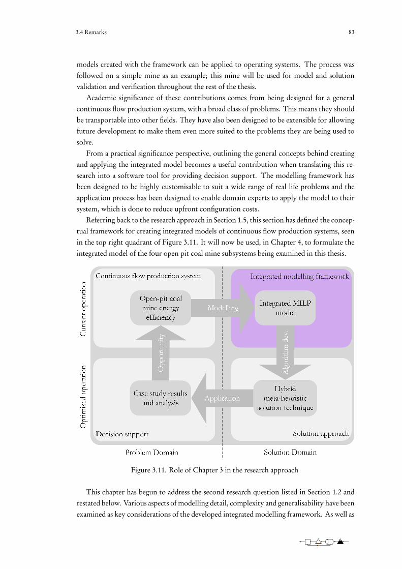
3.4 Remarks 83
models created with the framework can be applied to operating systems. The process wasfollowed on a simple mine as an example; this mine will be used for model and solutionvalidation and verification throughout the rest of the thesis.
Academic significance of these contributions comes from being designed for a generalcontinuous flow production system, with a broad class of problems. This means they shouldbe transportable into other fields. They have also been designed to be extensible for allowingfuture development to make them even more suited to the problems they are being used tosolve.
From a practical significance perspective, outlining the general concepts behind creatingand applying the integrated model becomes a useful contribution when translating this re-search into a software tool for providing decision support. The modelling framework hasbeen designed to be highly customisable to suit a wide range of real life problems and theapplication process has been designed to enable domain experts to apply the model to theirsystem, which is done to reduce upfront configuration costs.
Referring back to the research approach in Section 1.5, this section has defined the concep-tual framework for creating integrated models of continuous flow production systems, seenin the top right quadrant of Figure 3.11. It will now be used, in Chapter 4, to formulate theintegrated model of the four open-pit coal mine subsystems being examined in this thesis.
Figure 3.11. Role of Chapter 3 in the research approach
This chapter has begun to address the second research question listed in Section 1.2 andrestated below. Various aspects of modelling detail, complexity and generalisability have beenexamined as key considerations of the developed integrated modelling framework. As well as

84 CHAPTER 3. MODELLING APPROACH
this, a process for applying the integrated models using this framework has been proposed.
2. What integrated optimisation model of energy efficiency is appropriate for an open-pit coalmine production system?
(a) What level of detail is required of the model?
(b) Where are the main points of model complexity?
(c) How general should the model be?
(d) What is an appropriate process for applying the model to a real life mine?

4Integrated Model
This chapter applies the modelling framework described in Chapter 3. Section 4.1 presents theMILP formulation of the integrated mine model, made up of the top level, ‘whole-of-mine’,notation, parameters, variables and constraints as well as the variables and constraints usedto model each subsystem. Section 4.2 then uses the simple example introduced in Section 3.3to validate the model. Finally some remarks about the model’s benefits and limitations aremade in Section 4.3.
85
86 CHAPTER 4. INTEGRATED MODEL
4.1 Formulation
The general integrated model of an open-pit coal mine is formulated using the methodologiesdescribed in Section 3.1. First, with the aid of the models reviewed in Section 2.4, the subsys-tem modules that were conceptually defined in Section 3.2 are formulated using MILP. Theseare then integrated into a single model by modelling the material flow connections, totalenergy consumption and tasks. To show how the integrated model has been built from thesubsystem modules, the representation below is broken up into variable and constraint groupsthat represent the different subsystems of the formulation, as well a group that represents thesystem-wide aspects of the formulation, referred to as the ‘whole-of-mine’.
As mentioned in Section 3.2, the subsystem modules have initially been formulated toemulate the current standard amongst the models in literature, reviewed in Section 2.4. Des-pite the potential drawbacks, highlighted in Section 2.4, of the excavation and haulage sub-system allocation models in literature, this study first creates the integrated model using anallocation formulation. Using this, the issues are first confirmed, and then used as motivationfor the proposed improvements in Chapter 6.

4.1 Formulation 87
4.1.1 Notation
Whole-of-mine
Q Set of subsystemsE Set of excavation and haulage subsystems ⊆QP Set of processing plant subsystems ⊆QV Set of stockpile subsystems ⊆QB Set of belt conveyor subsystems ⊆QIq Set of inlet connection points on subsystem q ∈QJq Set of outlet connection points on subsystem q ∈QK Set of all connection points
⋃
q∈QIq ∪ Jq
C Set of connections (a pair of one outlet and one inlet connection point)A Set of tasksT Set of operating statesG Set of material types / gradesq Subsystem ∈Qqe Excavation and haulage subsystem ∈ Eqp Processing plant subsystem ∈ Pqv Stockpile subsystem ∈Vqb Belt c"onveyor subsystem ∈ Bi Inlet connection point ∈ Iq
j Outlet connection point ∈ Jq
k Connection point, ∈Kc Connection, ∈Cc in Inlet connection point of connection c ∈Ccout Outlet connection point of connection c ∈Ca Task, ∈At Operating state, ∈ Tg Material type / grade, ∈G
Excavation and haulage, ∀qe ∈ E
DqeSet of grades extracted from pits ⊆G
RqeSet of trucks
SqeSet of shovels
r Truck, ∈ Rqe
s Shovel, ∈ Sqe

88 CHAPTER 4. INTEGRATED MODEL
Processing plant, ∀qp ∈ P
B rawqp
Set of raw ore grades able to be processed, ⊆G
Bprodqp
Set of product grades, ⊆G
pprodqp
Product outlet connection point, ∈ Jqp
pwasteqp
Waste outlet connection point, ∈ Jqp
b wasteqp
Grade of waste output from pwasteqp
, ∈G
Stockpile, ∀qv ∈V
B stockedqv
Set of ore grades stockpiled, ⊆G
There are no belt conveyor sets or indices.
4.1.2 Parameters
Whole-of-mine
Ht Time span of state t (hours)ζ start
a State which task a starts in, ∈ Tζ stop
a State which task a stops in, ∈ Tζ min
a Minimum mass transferred for task a (tonnes)ζ max
a Maximum mass transferred for task a (tonnes)ζ grade
a Material type / grade transferred for task a, ∈Gζ con.p
a Connection point of transferred mass for task a, ∈K
Excavation and haulage, ∀qe ∈ E
cdtj i qe
Trip time of trucks driving from j to i (hours)
cdbi j qe
Trip time of trucks driving from i to j (hours)
c li g s qe
Loading time of shovel s at pit i extracting grade g ∈Dq (hours)γr qe
Payload of truck r (tonnes)αtdt
j i r qeTruck r energy usage per hour driving from j to i (MW)
αtdbi j r qe
Truck r energy usage per hour driving from i to j (MW)
αtlr qe
Truck r energy usage per hour idle (MW)αsl
s qeShovel s energy usage per hour loading (MW)
αsis qe
Shovel s energy usage per hour idle (MW)

4.1 Formulation 89
Processing plant, ∀qp ∈ P
σg g ′qpFraction of g ∈G required to produce g ′ ∈ Bprod
q (tonnes/tonne)
ηminqp
Minimum rate of production output (tonnes/hour)ηmax
qpMaximum rate of production output (tonnes/hour)
αppfixedqp
Fixed energy usage of plant when operating (MW)αppvar
qpVariable energy usage of plant when operating (MW/(t/h))
αpppcqp
Energy usage of positive changes to plant load (MWh/(t/h))αppnc
qpEnergy usage of negative changes to plant load (MWh/(t/h))
Stockpile, ∀qv ∈V
πstackqv
Maximum rate of stacking (tonnes/hour)πreclaim
qvMaximum rate of reclaiming (tonnes/hour)
λming qv
Minimum level of grade g ∈ B stockedqv
pile (tonnes)λg0qv
Initial (state 0) level of grade g ∈ B stockedqv
pile (tonnes)αstack
qvEnergy usage coefficient of stacking (MW/(t/h))
αreclaimqv
Energy usage coefficient of reclaiming (MW/(t/h))
Belt conveyor, ∀qb ∈ B
πbeltqb
Maximum rate of flow over belt (tonnes/hour)αbelt
qbEnergy usage coefficient of belt conveyor (MW/(t/h))
4.1.3 Decision variables
Whole-of-mine
θk g t Mass flow of grade g through connection point k in state t (tonnes/hour)zt q Energy usage of subsystem q in state t (MWh)
Excavation and haulage, ∀qe ∈ E
ni j g s r t qenumber of trips r takes of g from s at i to j in state t
νi j g r t qeFlow of g truck r moves from i to j in state t (tonnes/hour)
yi s qe=
⎧
⎨
⎩
1 when shovel s is allocated to pit i
0 otherwise
u truckr t qe
=
⎧
⎨
⎩
1 when truck r is allocated in state s
0 otherwise
Processing plant, ∀qp ∈ P
wg t qp=
⎧
⎨
⎩
1 when plant is producing grade g ∈ Bprodqp
in state t
0 otherwise

90 CHAPTER 4. INTEGRATED MODEL
d+g t qpPositive change in production of grade g ∈ Bprod
qp(tonnes/hour)
d−g t qpNegative change in production of grade g ∈ Bprod
qp(tonnes/hour)
Stockpile, ∀qv ∈V
λg t qvLevel of g ∈ B stocked
qvpile at the end of state t (tonnes)
There are no belt conveyor decision variables, its operation is determined by the mass flowthrough its connection points, represented by θk g t , the whole-of-mine decision variable.
4.1.4 Objective
Minimise ∑
∀t ,q
zt q (4.1)
The objective function, (4.1), represents the total energy usage, in MWh, of the mine forminimisation. Each subsystem is responsible for defining its energy usage, zt q ; these are allexpressed as equality constraints in the following section.
4.1.5 Constraints
Whole-of-mine
These constraints apply at the top, whole-of-system, level of the model where subsystems areconnected to one another and work together to achieve the planned tasks.
θcout g t = θc in g t ∀c , g , t (4.2)
ζ stopa∑
t=ζ starta
h
Htθζ con.pa ζ grade
a t
i
≥ ζ mina ∀a (4.3)
ζ stopa∑
t=ζ starta
h
Htθζ con.pa ζ grade
a t
i
≤ ζ maxa ∀a (4.4)
θk g t = 0 ∀k , t , g (4.5)
zq t = 0 ∀q , t (4.6)
Constraint (4.2) balances the inlet and outlet connection points of each connection in themodel. Constraint (4.3) and (4.4) set the minimum and maximum amount of work requiredby each task, respectively. Constraint (4.5) and (4.6) ensure non-negative mass flows andenergy consumptions, respectively.
Excavation and haulage
As mentioned previously, the excavation and haulage subsystem is first modelled using anallocation formulation based on recent literature (Mena et al., 2013; Sahoo et al., 2014; Souza

4.1 Formulation 91
et al., 2010; Ta et al., 2013). Shovels are allocated to pits and trucks are allocated trips fromshovels at those pits to destinations. They work together to dig raw material from the groundand deliver it to the required destinations. Due to the complex nature of the excavationand haulage operation and data availability for the case study, it has the most sophisticatedformulation of the four subsystems.
The operation of the subsystem is parameterised by the loading and driving times itsequipment achieves when working at particular pits; the truck payloads; and the energy eachindividual equipment piece consumes while performing different activities. It is important tocharacterise the energy parameters of each truck individually to ensure the allocated truckswill be the most energy efficient. This can also improve the performance of the optimisation,as it reduces the amount of symmetry in the solution space.
∑
∀i , j ,g ,s
ni j g s r t qe
�
cdtj i qe+ c l
i g s qe+ cdb
i j qe
�
≤Ht u truckr t qe
∀r, t , qe (4.7)
∑
∀i
yi s qe≤1 ∀s , qe (4.8)
∑
∀ j ,r
ni j g s r t qe≤
⎢
⎢
⎢
⎣
Ht
c li g s qe
⎥
⎥
⎥
⎦ yi s qe∀i , g , s , t , qe (4.9)
νi j g r t qe=γr qe
ni j g s r t qe
Ht∀i , j , g , r, t , qe (4.10)
θi g t =∑
∀ j ,r
νi j g r t qe∀i , g , t , qe (4.11)
θ j g t =∑
∀i ,r
νi j g r t qe∀ j , g , t , qe (4.12)
zt qe=∑
∀r
αtlr qe
⎡
⎣Ht u truckr t qe−
∑
∀i , j ,g ,s
ni j g s r t qe
�
cdtj i qe+ cdb
i j qe
�
⎤
⎦
+∑
∀i , j ,g ,s
ni j g s r t qe
�
αtdtj i r qe
cdtj i qe+αtdb
i j r qecdb
i j qe
�
+∑
∀i , j ,g ,s ,r
αsls qe
c li g s qe
ni j g s r t qe
+∑
∀i ,s
αsis qe
⎡
⎣Ht yi s qe−∑
∀ j ,g ,r
c li g s qe
ni j g s r t qe
⎤
⎦
∀t , qe (4.13)
Constraint (4.7) ensures a truck isn’t allocated for more than the available time in eachstate. Constraint (4.8) ensures shovels are allocated only once. Constraint (4.9) sets therelationship between ni j g s r t qe
and yi s t qeand limits the number of trucks allocated to a pit
over time to avoid wasteful queues and over allocation of shovels. Constraints (4.10), (4.11)and (4.12) translate the allocations into mass flow rates for the subsystem’s inlet and outletconnection points. Constraint (4.13) represents the energy consumption of the excavationand haulage subsystem; made up of truck idle energy consumption, truck driving energy

92 CHAPTER 4. INTEGRATED MODEL
consumption, energy from shovel loading and the idle energy consumption of the shovel.Trucks are considered idle for all times they are not driving, during a state they’re used in.
Processing plant
A general formulation of the processing plant, extended from Middelberg et al. (2009), hasbeen developed to align with the objective of creating a generic enough model for reusabilityon other mines and to suit the limited data available for the case study in this thesis. Theformulation assumes known ratios for inlet grades (including water) to outlet product gradesand waste and decides the product grade output and how much is produced.
θpprod
q p g t≥wg t qp
ηminqp
∀g ∈ Bprodqp
, t , qp (4.14)
θpprod
q p g t≤wg t qp
ηmaxqp
∀g ∈ Bprodqp
, t , qp (4.15)∑
∀g∈Bprodq p
wg t qp≤1 ∀t , qp (4.16)
σg g ′qpθ
pprodq p g ′ t
=∑
∀i
θi g t ∀g , g ′ ∈ Bprodqp
, t , qp (4.17)
θpwasteq p b waste
q p t =∑
∀i ,g
θi g t −∑
∀g∈Bprodq p
θpprod
q p g t∀t , qp (4.18)
d+g t qp− d−g t qp
=θpprod
q p g t−θ
pprodq p ,g ,t−1
∀g ∈ Bprodqp
, t < |T |, qp (4.19)
zt qp=Ht
∑
∀g∈Bprodq p
�
αppfixedqp
wg t qp+αppvar
qpθ
pprodq p g t
+αpppcqp
d+g t qp+ αppnc
qpd−g t qp
i
∀g ∈ Bprodqp
, t < |T |, qp (4.20)
Constraints (4.14) and (4.15) sets the minimum and maximum operating capacity, respect-ively, as well as the boolean variable for the operating mode of plant, wg t qp
. This booleanvariable is further constrained in (4.16), which ensures a maximum of one grade is producedat a time. Constraints (4.17) and (4.18) are mass balances for product output and wasteoutput, respectively. Constraint (4.19) sets the positive and negative changes in productionrate between states. Constraint (4.20) sets the energy consumption of the plant, made up offixed consumption when in operation, a variable consumption proportional to the plant loadand the extra energy consumed due to changing the plant load between states.
Stockpile
The stockpile formulation has been developed to apply to many different stockpiles. A net-work flow model with inventory is used as the basis for the formulation, similar to Ta et al.(2005) and Hanoun et al. (2013). Multiple grades can be stored by each stockpile subsystem.

4.2 Validation 93
∑
∀i ,g
θi g t ≤πstackqv
∀t , qv (4.21)
∑
∀ j ,g
θ j g t ≤πreclaimqv
∀t , qv (4.22)
λg t qv≥λmin
g qv∀g ∈ B stocked
qv, t , qv (4.23)
λg t qv=λg ,t−1,qv
m
+Ht
∑
∀i
θi g t
−Ht
∑
∀ j
θ j g t
∀g ∈ B stockedqv
, t , qv (4.24)
zt qv=Htα
stackqv
∑
∀i ,g
θi g t
+Htαreclaimqv
∑
∀ j ,g
θ j g t
∀t , qv (4.25)
Maximum stacking and reclaiming rates are enforced by constraints (4.21) and (4.22)respectively. Constraint (4.23) places a minimum allowable stockpile level for each storedgrade. Constraint (4.24) represents the mass balance of the subsystem, including the holdupof stocked material. The energy consumption of the stacking and reclaiming activity isexpressed in Constraint (4.25).
Belt conveyor
Belt conveyors are formulated as network flow models without inventory constraints, similarto Middelberg et al. (2009).
θ∀i ,g ≤πbeltqb
∀t , qb (4.26)∑
∀i
θi g t =∑
∀ j
θ j g t ∀g , t , qb (4.27)
zt qb=Htα
beltqb
∑
∀i ,g
θi g t ∀g ∈ B stockedqv
, t , qb (4.28)
Constraint (4.26) represents the maximum mass flow rate over belt conveyor. Constraint(4.27) is the mass balance equality for the subsystem and the energy usage, proportional toload, is set in Constraint (4.28).
4.2 Validation
In this section the simple example mine that demonstrated the application process in Sec-tion 3.3 will be used to validate the results of the integrated model presented in the previoussection. For all instances in this section, the model has been solved using IBM CPLEX

94 CHAPTER 4. INTEGRATED MODEL
Optimizer on an Intel i7 CPU with 16GB of RAM. The first problem instance comes fromfitting the model with the parameters and tasks as they are described in Section 3.3. Two 1-hour time states are used and the tasks are re-listed below in Table 4.1. The problem instancehas 928 variables and 789 constraints; it is solved to optimality in 468.43 seconds.
Table 4.1. Simple example task list
Task #Connection
pointMaterial grade Amount (t)
Start time(hr)
End time(hr)
1 Extraction pit 1 ROM 3,000 0 22 Extraction pit 2 Overburden 3,000 0 2
3Processing plantproduct outlet
Product 2,000 0 2
The subsystem energy usages are reported in Table 4.2. It can be seen that the largestconsumers of energy are the extraction subsystem and processing plant, which is consistentwith expectations.
Table 4.2. Energy consumption (MWh)
SubsystemState 1(0-1hr)
State 2(1-2hr)
Alltime
Belt conveyor 0.15 0.15 0.29Extraction 9.03 7.72 16.75Pit 1 0.00 0.00 0.00Pit 2 0.00 0.00 0.00Processing plant 8.52 8.52 17.05Stockpile 0.29 0.15 0.44Waste dump 1.06 0.93 1.99Whole mine 19.05 17.47 36.52
Table 4.3 shows the material transferred over each connection between the subsystemsand on the model’s boundary connection points. The three production targets, underlined,that are entered as input into the model as tasks have all been met. The overall excavationand haulage work is fairly evenly split between the two hours, with slightly more work beingdone in the first state. This is reflected in where the processing plant gets its ROM input. Theprocessing plant input is supplemented by the ROM stockpile more in the second hour whenthe haulage and excavation reduces its ROM extraction, which is the expected behaviour of anoperating mine. This validates that the mass balance constraints across the various subsystemsare working as expected.

4.2 Validation 95
Table 4.3. Total material transferred (tonnes)
Connection GradeState 1(0-1hr)
State 1(1-2hr)
All time
belt conveyor out Product 1,000.00 1,000.00 2,000.00extraction→processing plant ROM 1,220.00 1,190.00 2,410.00extraction→stockpile ROM 440.00 220.00 660.00extraction→waste dump Ovb. 1,600.00 1,410.00 3,010.00extraction pit 1 in ROM 1,660.00 1,410.00 3,070.00extraction pit 2 in Ovb. 1,600.00 1,410.00 3,010.00processing plant→belt conveyor Product 1,000.00 1,000.00 2,000.00processing plant tailings out Tailings 292.15 292.15 584.30processing plant water in Water 69.15 69.15 138.30stockpile→processing plant ROM 3.00 33.00 36.00
Table 4.4 shows the truck allocations over the period. The number of times it makes aparticular trip (inlet/outlet pair) is displayed for each state. There are 26 trips made across thetwo hours. ROM is being extracted from pit 1; ten trips are made to the processing plant (PP)and three are made to the stockpile (SP). The remaining thirteen are transporting overburden(Ovb.) from pit 2 to the waste dump (WD). Truck 3, the least efficient truck, is not used atall, while truck 5 is only used in the first hour. The other trucks all make six trips each, threein each hour.
Table 4.4. Truck allocation
State State 1 (0-1hr) State 1 (1-2hr)Shovel 1 2 1 2 AllGrade Ovb. ROM Ovb. ROM timeInlet Pit 2 Pit 1 Pit 2 Pit 1 &
Outlet WD PP SP WD PP SP tripsTruck 1 1 2 0 0 3 0 6Truck 2 1 2 0 3 0 0 6Truck 3 0 0 0 0 0 0 0Truck 4 2 0 1 1 1 1 6Truck 5 1 0 1 0 0 0 2Truck 6 2 1 0 2 1 0 6
All trucks 7 5 2 6 5 1 26
To further analyse the model, instances of varying sizes have been solved. Table 4.5 showsthe objective values and CPU times from solving several small instances based on the simpleexample introduced in Section 3.3. They have been solved to optimality with CPLEX, thecomputation times are also listed.

96 CHAPTER 4. INTEGRATED MODEL
Table 4.5. Computational results (simple example instances)
id states shovels trucks pit target (t)product
target (t)obj.
(MWh)CPU
sec.4.01 1 1 2 (1500) 1,000 12.70 0.274.02 1 1 4 (2500) 2,000 22.34 0.264.03 1 1 6 (3250) 2,000 24.15 0.274.04 1 2 2 (750, 500) 500 9.75 0.344.05 1 2 4 (1000, 1000) 500 12.94 0.364.06 1 2 6 (1500, 1500) 1,000 19.10 0.264.07 2 1 2 (3000) 2,000 25.39 0.264.08 2 1 4 (5000) 4,000 43.19 0.264.09 2 1 6 (7000) 6,000 61.54 0.264.10 2 2 2 (1000, 1000) 500 16.77 0.374.11 2 2 4 (2000, 2000) 1,000 24.38 1.164.12 2 2 6 (3000, 3000) 2,000 36.52 468.43
As these instances do not reflect practically sized problems, they do not give an indicationof the effectiveness of CPLEX as a solution approach. Using the case study, described in detailin Chapter 5, several more instances are solved to examine the quality and speed of CPLEX fora more realistic problem size. Table 4.6 describes the problem instances to give an indicationof size. For these problems, 2 hour operating states are used. Table 4.7 presents the results ofsolving the CPLEX with a 1-hour and 2-minute time limit, as well as the best known lowerbound (LB) reported by CPLEX.
Table 4.6. Case study instance descriptions
id states shovels trucks pit target (t)product
target (t)4.13 2 2 10 (5000, 5000) 1,0004.14 2 2 15 (7500, 7500) 2,5004.15 2 2 20 (10000, 10000) 5,0004.16 2 4 10 (2500, 2500, 2500, 2500) 1,0004.17 2 4 15 (3750, 3750, 3750, 3750) 2,5004.18 2 4 20 (5000, 5000, 5000, 5000) 4,0004.19 4 2 10 (10000, 10000) 2,5004.20 4 2 15 (15000, 15000) 5,0004.21 4 2 20 (20000, 20000) 10,0004.22 4 4 10 (5000, 5000, 5000, 5000) 2,0004.23 4 4 15 (7500, 7500, 7500, 7500) 5,0004.24 4 4 20 (10000, 10000, 10000, 10000) 8,000

4.2 Validation 97
Table 4.7. Computational results (case study instances)
CPLEX 1hr time limit CPLEX 2min time limit
id
Bestknown
LB(MWh)
obj.(MWh)
% gapobj.
(MWh)% gap
4.13 65.40 65.40 0.00% 65.40 0.00%4.14 90.01 90.19 0.20% 90.20 0.21%4.15 128.27 128.54 0.21% 128.55 0.22%4.16 73.11 73.27 0.22% 73.27 0.22%4.17 99.34 99.51 0.17% 99.51 0.17%4.18 132.85 133.09 0.18% 133.09 0.18%4.19 130.75 131.01 0.20% 131.01 0.20%4.20 179.76 180.15 0.22% 180.23 0.26%4.21 255.98 256.82 0.33% 256.82 0.33%4.22 145.08 145.38 0.21% 145.38 0.21%4.23 197.49 197.95 0.23% 198.01 0.26%4.24 265.13 265.79 0.25% 265.79 0.25%
It is clear from Table 4.7 that CPLEX is able to find a good quality solution within 2minutes to these instances. This indicates it is an appropriate method for solving the model forpractical sized problems. It will therefore be used to solve the case study analysis in Chapter 5.
4.2.1 Issues
While the model produces sensible solutions and justifies its application to a real life casestudy, there are a number of drawbacks of using allocation to model the excavation andhaulage subsystem that will impact its accuracy, as mentioned in Subsection 2.4.2 of theliterature review. They relate to the lack of sequence and time information considered inthe formulation.
The issues can be demonstrated using the first instance, 4.01, from the above computa-tional analysis. For this instance, the optimal result involves 6 trips, three from each truck.Table 4.8 shows the trips they are required to make.
Table 4.8. Instance 4.01 truck allocations
State State 1 (0-1hr)Shovel 1Grade ROMInlet Pit 1
Outlet PP SPTruck 1 3 0Truck 2 2 1
All trucks 5 1
Since these trips are all to a single shovel, they physically cannot happen at the same time.This means they must happen in sequence. However, the current, allocation based, model

98 CHAPTER 4. INTEGRATED MODEL
formulation doesn’t indicate the sequence. This results in accuracy limitations that impactboth optimality and feasibility.
The first is that the time between different trips may be different, which will thereforeimpact the amount of time the truck is driving. This is illustrated in Figure 4.1 by consideringtwo of the trips truck 2 needs to make – pit 1 to the processing plant and pit 1 to the ROMstockpile – and applying the driving time parameters outlined in Subsection 3.3.5. From thissimple example, it is clear that different trip sequences may result in differences in drivingtimes. By not considering this properly, the accuracy of the objective and feasibility areboth impacted. Firstly, the truck driving component of the objective will not take intoconsideration the potential differences in driving times. Secondly, if these differences in timesare large enough, it may be the difference between enough and not enough time for a trip tohappen feasibly.
Figure 4.1. Driving time differences between trip orders
The second issue is that the model cannot properly account for truck waiting time. Thiscan be demonstrated by manually scheduling the trips described in Table 4.8. Figure 4.2,Figure 4.3 and Figure 4.4 illustrate three possible schedules that result from sequencing theoptimal truck allocations from instance 4.01. Black indicates the times when trucks are beingloaded by shovels; the coloured blocks represent when trucks are loaded and driving to thedestination; grey blocks of time are when the truck is then driving from its last destinationto the next pit; time between grey and the next loading is when trucks are waiting. It isclear from these three possible schedules that the sequence can have a large impact on truckwaiting time. This will impact accuracy of both the optimality and feasibility. Trucks waitingat shovels will consume idle energy that isn’t currently accurately being accounted for in theobjective function. Depending on the amount of truck waiting time, the ability for a giventrip to happen in a state can also be impacted, which may cause infeasibilities.

4.2 Validation 99
Figure 4.2. Instance 4.01 – Feasible schedule 1
Figure 4.3. Instance 4.01 – Feasible schedule 2

100 CHAPTER 4. INTEGRATED MODEL
Figure 4.4. Instance 4.01 – Feasible schedule 3
Another issue that is demonstrated in the above schedules, is the ability to properly con-sider the trucks travelling from base at the start, back to base at the end, and potentially toand fro during the shift. This is also not being considered by the current formulation.
4.3 Remarks
This chapter has successfully applied the conceptual methodology described in Chapter 3and presented an integrated model of an open-pit coal mine. The four subsystems have beenformulated in line with models from recent literature and integrated into a single MILP for-mulation. The modelling framework has been shown to be effective at decoupling subsystemformulations and supporting model generalisation to allow for application to different mines.
While validation of the model showed it produces sensible results, issues with the excava-tion and haulage allocation formulation have been highlighted. A small problem instance hasbeen analysed to demonstrate the issues. They relate to the fact that the allocation formulationdoes not give the sequence or times of truck trips from shovels to destinations.
The first is that a truck making different trip types may drive for different amounts of timedepending on the sequence in which it does the trips. Since the time of a trip being allocatedto a truck isn’t known for sure without sequence, the energy of driving cannot be accuratelymodelled in the objective, and the feasibility of assigning trucks to trips cannot be guaranteed.
The second issue is related to the synchronicity between trucks and shovels. Withoutknowing the order and time of trips, the formulation cannot properly model the loadinginteraction between the shovels and trucks. Most importantly this means waiting times arenot accounted for, which also impacts the objective value and feasibility.
While these issues are important to overcome, the model can still give useful results for

4.3 Remarks 101
providing decision support to operators for making energy efficiency improvements, as dothe other models in literature with similar limitations. Hence before they are overcome, areal life case study will be analysed with the model presented in this chapter. This will alsobe useful for reinforcing the importance of improving the model by asserting their existencein a real life application.
The contribution of this chapter, referring back to the research approach described in Sec-tion 1.5, relates to the inner part of the top right quadrant of Figure 4.5. Since the model in itscurrent form does not appear too complex for exact techniques to solve optimally in practicaltime for real life sized problems, the bottom right quadrant of Figure 4.5 can be triviallyreplaced with the IBM CPLEX Optimizer for now. This does not mean the complexity andsolution approach related hypotheses have been disproved. Rather, the research approachwas designed to be an iterative process. Due to the limitations of the model presented in thischapter and expanded upon in the next, the model will be revisited in Chapter 6 to formulatean improved, complex model, which will require the work earmarked by the bottom rightquadrant of Figure 4.5 to properly further test the hypotheses.
Figure 4.5. Role of Chapter 4 in the research approach
This chapter has further addressed research questions 2a, 2b and 2c from Section 1.2, listedbelow, by using the modelling framework to build a formulation with various levels of detail,complexity and generalisability. The excavation and haulage subsystem is where the majorityof detail and complexity exists in the model and is also where accuracy issues have arisen. Thiswill be the focus of later improvements where these questions will be revisited again.
2. What integrated optimisation model of energy efficiency is appropriate for an open-pit coal

102 CHAPTER 4. INTEGRATED MODEL
mine production system?
(a) What level of detail is required of the model?
(b) Where are the main points of model complexity?
(c) How general should the model be?

5Case Study
This chapter conducts a case study on a real life open-pit coal mine to verify and validate thedeveloped model and methodologies. The mine being studied is an open-pit coal mine insouth east Queensland, Australia, named Meandu Mine.
All of the product coal produced by Meandu Mine is delivered via belt conveyor to TarongPower Station, an adjacent coal-fired power station. The mine and power station are bothowned by Stanwell Corporation, a Queensland Government owned corporation. A private,company, Downer Mining, a subsidiary of Downer EDI Limited, is contracted by Stanwellto operate the mine. The data and information provided for this case study has come fromcontacts within Downer Mining working at Meandu Mine.
This chapter first follows the process described in Section 3.3 to fit the integrated modelpresented in Section 4.1 to the mine. It then details the results of a scenario analysis thathas been conducted to verify and validate the accuracy of the model and its solutions. Thechapter concludes by highlighting issues with the current model that were found throughoutthe results which motivate modifications made in the next chapter.
103

104 CHAPTER 5. CASE STUDY
5.1 Apply the integrated model
5.1.1 Gather production system information
Information about Meandu Mine was gathered from a number of different sources. Variousreports and plans were provided upfront from the mine. This was followed by a mine visitthat involved discussion with managers from both the extraction and CHPP sides of the mineand a tour of the mine through the majority of its operations. The initial provision of datawas very useful in ensuring relevant and valuable discussion could be had during the minevisit. Together, these formed enough information to answer all the necessary questions in thefirst step of the application process, and were valuable for the later stage of parameterising themodel.
The remainder of this section will outline the answers to the questions described in Sub-section 3.3.1.
Whole-of-mine questions
What are the boundaries of the mine?
The following figures are satellite images of Meandu Mine. Figure 5.1 shows thewhole mine, while Figure 5.2 shows just the CHPP setup of the mine, boxed inred in Figure 5.1).
The mine extracts from five pit faces, and has one product load out belt conveyor.

5.1 Apply the integrated model 105
Figure 5.1. Meandu mine satellite image (Maps, 2014)

106 CHAPTER 5. CASE STUDY
Figure 5.2. Meandu mine CHPP satellite image (Maps, 2014)
What systems perform the majority of the work?
Meandu is a fairly typical open-pit coal mine, it has a drilling and blasting opera-tions, dragline, loaders extracting the material from the face, trucks transportingit to be handled or dumping waste, and a CHPP.
The CHPP at Meandu Mine could be considered as a single subsystem, however,there is a stockpile between the crusher and wash plant, and so for the purposesof this case study, to get a better picture of the activity of the CHPP operation,two processing plants will be considered (a crusher and a wash plant) along withthe intermediate stockpile and a number of belt conveyors.
What are the main energy consumers of the mine?
The energy is primarily consumed by the operations listed in the above question.
How many different types material are transported between systems?

5.1 Apply the integrated model 107
There are a number of different materials which are handled throughout the mainoperations of the mine, these are:
• Run of Mine (ROM) coal
• Crushed ROM coal
• Product coal
• Overburden
• Spoil (similar to overburden)
• Top soil
• Tailings
• Water
Note: Spoil is overburden material that has been dumped on previously uneco-nomical coal, which has now been determined to be economical. The distinctionbetween spoil and overburden is made by the mine since spoil is already soft anddoes not need to be blasted. This is an example of the external factor, ‘operationalhistory’, mentioned SubSection 2.3.7, having an impact on current operation.
Excavation and haulage questions
What are the boundaries of the subsystem?
There are five pit faces that are extracted from. These make up the inlets to theextraction subsystem.
The ROM coal is delivered either to a stockpile or directly to a belt conveyorgoing to the CHPP; these make up the first two outlets of the extraction system.
On top of those outlets, there are a number of places that are used to dump wastematerial. While there are more than five destinations for waste it is not normalfor the mine to be delivering to all of them, so only a few are required; for thepurposes of this model, there will be three waste dumps for overburden and spoil,and one top soil waste dump.
This makes for six outlets.
What grades are being extracted?
ROM coal, overburden, spoil and top soil are the grades being extracted from thepits.
How many loaders are there?
There are four loaders: two EX3600 Hitachi Excavators, one EX5500 HitachiExcavator and one EX3500 Hitachi Shovel.

108 CHAPTER 5. CASE STUDY
How many trucks are there?
There are 20 trucks, six Komatsu 830E DC, eight Komatsu 630E DC and sixKomatsu 830E AC.
Processing plant questions
As mentioned earlier, two processing plants are being considered for this modelling exercise:the crusher and wash plant.
What are the boundaries of the subsystem?
The crusher is fed a belt conveyor and outputs to another belt conveyor.
The wash plant is also fed input material from a single conveyor, has anotherinput for water and has two outputs, one for product and the other for tailings.
What materials can be processed?
The crusher processes ROM coal from the pits.
The wash plant processes crushed ROM coal and also consumes water.
What materials are produced?
Crushed ROM coal is produced by the crusher.
Product coal and tailings are output from the wash plant.
Stockpile questions
There are seven stockpile subsystems being considered for the model, five of which are differ-ent waste dumps, the sixth is for ROM coal and the seventh is for crushed ROM coal. Thereis no storage of product at Meandu Mine.
What are the boundaries of the subsystem? /What grades are stored in the stockpile?
The five waste dumps each have only a single input, delivering the waste materialfrom either trucks (for the top soil dump and three waste dumps) or from theconveyor transporting tailings out of the wash plant. The top soil dump is filledwith top soil material. The three regular waste dumps are filled with eitheroverburden or spoil material. The tailings dump is filled with tailings material.
The ROM stockpile has a single inlet, being fed from the extraction subsystemand a single outlet feeding the crusher inlet conveyor. It stores ROM coal mater-ial.
The crushed ROM stockpile has a single inlet from the crusher outlet conveyorand a single outlet to the wash plant inlet conveyor. It stores crushed ROM coalstraight from the crusher.
5.1 Apply the integrated model 109
Belt conveyor questions
There are five conveyors being considered for the Meandu Mine mode.
What are the boundaries of the subsystem? / What grades can be transported over the belt con-veyor?
The conveyor transporting ROM coal to the crusher has two inlets coming fromthe extraction subsystem and the ROM stockpile and has a single outlet feedingthe crusher. It transports ROM coal.
Crushed ROM coal can bypass washing and be fed directly to the product loadout conveyor; therefore the conveyor that has the crusher output as its inlet hastwo outlets, one going to the crushed ROM stockpile, the other to the productdelivery conveyor. It transports crushed ROM coal.
The conveyor between the crushed ROM stockpile and the wash plant has a singleinlet and a single outlet. It transports crushed ROM coal.
The conveyor transporting tailings out of the wash plant to the tailings dumpalso has a single inlet and a single outlet. It transports tailings material.
The product delivery conveyor is fed by either the crusher outlet conveyor orfrom the wash plant and has a single outlet to Tarong Power Station, whichrepresents the output boundary of the whole mine model. It transports eitherproduct coal or crushed ROM coal.
Other subsystem questions
There are no other subsystems required to be modelled for this case study.
5.1.2 Outline process flow of system
Using the information gathered in step one of the process, the process flow of the systembeing modelled can be determined. Figure 5.3 is a process flow diagram (PFD) representingeach subsystem that will be modelled and the material connections between them.

110 CHAPTER 5. CASE STUDY
Figure 5.3. Meandu mine process flow diagram (Maps, 2014)

5.1 Apply the integrated model 111
5.1.3 Formulate new subsystem model(s) (if required)
Each of these subsystems can be modelled with one of the four modules developed for thisresearch, so there is no requirement for new subsystem modelling.
5.1.4 Apply structural information to integrated model
By examining the gathered information and generated process flow diagram, each of thesets, which define the structure of the integrated model, can now be defined. The tables inAppendix A show the values entered for each of the sets.
5.1.5 Enter subsystem parameter values
See Appendix B for data tables containing the parameter values for each subsystem.
5.1.6 Enter shift production targets and define operating states
A monthly production plan was provided by Meandu Mine. A typical 8 hour time periodwas selected from the plan and the activities relevant to the modelled operations of the minewere entered as tasks, seen in Table 5.1.
Table 5.1. Production target tasks
Task#
Start time(hr)
Stop time(hr)
Grade Connection Mass (t)
1 0 8 Overburden Extraction pit 1 inlet 8,0002 0 8 ROM Extraction pit 2 inlet 10,0003 0 8 Spoil Extraction pit 3 inlet 14,0004 0 8 Product Wash plant outlet 8,000
A time resolution of two-hour steps over the eight hour period of production will be usedfor this case study. This has been selected as a reasonable resolution to reflect the on-sitedecisions which the model aims to provide assistance for.
5.1.7 Formulate new task(s) (if required)
Each of the four tasks detailed above fit into the existing model of a task, so no new tasks arerequired to be modelled for this case study.
5.1.8 Solve
Solving this model can be performed with IBM ILOG CPLEX. An Intel i7 CPU with 16GBof RAM for 2 minutes is used to find the solutions. Section 5.3 presents the results obtainedby solving the model using the production targets mentioned previously, along with somescenario analysis.

112 CHAPTER 5. CASE STUDY
5.2 Additional constraints
Following the model application process worked well for creating the integrated model of theprimary operations of the case study mine. There are, however, three extra sets of constraintsthat the model has been appended with, to make it represent the case study mine’s operationmore realistically.
The first additional constraints, 5.1–5.4, set the shovel allocation decision variables toknown locations. This was done since Meandu already knows their shovel allocations inadvance as part of their plan, and is therefore not an operational decision, so not requiredto be a decision variable for this particular model. Constraint 5.1 allocates shovel 1 to pit 2;Constraint 5.2 allocates shovel 2 to pit 3; Constraint 5.3 ensures shovel 3 is allocated to nopits; and Constraint 5.4 allocates shovel 4 to pit 1.
ypit 2,shovel 1,t ,qe=1 ∀t (5.1)
ypit 3,shovel 2,t ,qe=1 ∀t (5.2)
yi ,shovel 3,t ,qe=0 ∀i , t (5.3)
ypit 1,shovel 4,t ,qe=1 ∀t (5.4)
The second set of constraints that have been added, Constraints 5.5 and 5.6, blocks theextraction subsystem from delivering waste to waste dump 2 and 3. Much like the shovelallocation constraint added, the destination of waste is known in advance as part of the mineplan and is therefore not an operational decision to be made. For this operating shift, all wasteis delivered to waste dump 1, and hence the flow into the other two waste dumps is set to zero.
θextraction→ waste dump 2,g ,t =0 ∀g ∈Dqe, t (5.5)
θextraction→ waste dump 3,g ,t =0 ∀g ∈Dqe, t (5.6)
The final extra constraints, 5.7 and 5.8, ensures the wash plant and crusher, respectively,are always on. This has been done to better reflect the actual operation of the two subsystemsat the mine.
wcrushed ROM,t ,crusher =1 ∀t (5.7)
wproduct,t ,wash plant =1 ∀t (5.8)
5.3 Results
The case study is first solved to find a benchmark for the analysis. Sensitivity to productdemand is then investigated, followed by an analysis of the impact each truck has on thesolution, and a look at the current issues with the model. IBM CPLEX Optimizer on an

5.3 Results 113
Intel i7 CPU with 16GB of RAM for 2 minutes is used to find the solutions. The CPLEXsolution gaps were below 1% for all instances.
5.3.1 Benchmark solution
Using the information provided by the mine’s operator, the benchmark solution for the restof the analysis was found. Table 5.2 shows the energy consumption of each subsystem. Usingthe general definition of energy efficiency introduced in Section 2.2 (product output dividedby energy input) the energy efficiency of this result is 35.46 product tonnes per megawatthour (Product t/MWh). The extraction subsystem accounts for the large majority of energyconsumption, which is in line with information from site. Second and third are the crusherand wash plant, respectively, which is also consistent with expectation.
Table 5.2. Benchmark energy consumption (MWh)
Subsystem State 1(0-2hr)
State 2(2-4hr)
State 3(4-6hr)
State 4(6-8hr) All time
ROM stockpile 0.00 0.29 0.01 0.01 0.32CB1 0.12 0.12 0.12 0.12 0.46CB2 0.46 0.46 0.46 0.46 1.85CB3 0.39 0.39 0.39 0.39 1.54CB4 0.67 0.67 0.67 0.67 2.66CB5 0.59 0.59 0.59 0.59 2.36Crushed ROM stockpile 1.97 1.97 1.97 1.97 7.89Crusher 7.18 7.18 7.18 7.18 28.72Extraction 35.36 31.88 34.34 31.40 132.98Tailings dump 0.06 0.06 0.06 0.06 0.23Top soil dump 0.00 0.00 0.00 0.00 0.00Wash plant 6.15 6.15 6.15 6.15 24.58Waste dump 1 6.00 5.00 5.85 5.17 22.02Waste dump 2 0.00 0.00 0.00 0.00 0.00Waste dump 3 0.00 0.00 0.00 0.00 0.00Whole mine 58.94 54.75 57.78 54.16 225.63
Table 5.3 shows the amount of material transferred over each connection. The demandand production targets have all been met and are marked in bold in the last column. TheROM stockpile increases from 21000 tonnes to 21256 tonnes, 1.2%, over the 8 hour period,indicating that the extraction targets are fairly well balanced with the product demand well.
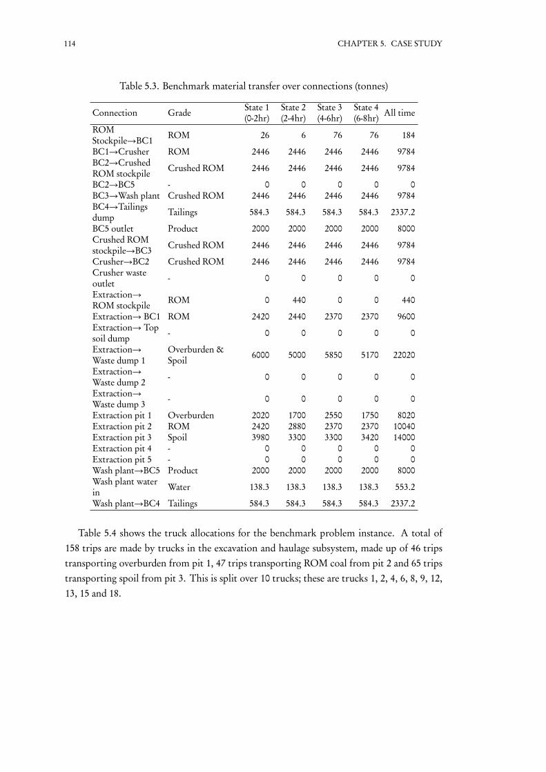
114 CHAPTER 5. CASE STUDY
Table 5.3. Benchmark material transfer over connections (tonnes)
Connection Grade State 1(0-2hr)
State 2(2-4hr)
State 3(4-6hr)
State 4(6-8hr) All time
ROMStockpile→BC1 ROM 26 6 76 76 184
BC1→Crusher ROM 2446 2446 2446 2446 9784BC2→CrushedROM stockpile Crushed ROM 2446 2446 2446 2446 9784
BC2→BC5 - 0 0 0 0 0BC3→Wash plant Crushed ROM 2446 2446 2446 2446 9784BC4→Tailingsdump Tailings 584.3 584.3 584.3 584.3 2337.2
BC5 outlet Product 2000 2000 2000 2000 8000Crushed ROMstockpile→BC3 Crushed ROM 2446 2446 2446 2446 9784
Crusher→BC2 Crushed ROM 2446 2446 2446 2446 9784Crusher wasteoutlet - 0 0 0 0 0
Extraction→ROM stockpile ROM 0 440 0 0 440
Extraction→ BC1 ROM 2420 2440 2370 2370 9600Extraction→ Topsoil dump - 0 0 0 0 0
Extraction→Waste dump 1
Overburden &Spoil 6000 5000 5850 5170 22020
Extraction→Waste dump 2 - 0 0 0 0 0
Extraction→Waste dump 3 - 0 0 0 0 0
Extraction pit 1 Overburden 2020 1700 2550 1750 8020Extraction pit 2 ROM 2420 2880 2370 2370 10040Extraction pit 3 Spoil 3980 3300 3300 3420 14000Extraction pit 4 - 0 0 0 0 0Extraction pit 5 - 0 0 0 0 0Wash plant→BC5 Product 2000 2000 2000 2000 8000Wash plant waterin Water 138.3 138.3 138.3 138.3 553.2
Wash plant→BC4 Tailings 584.3 584.3 584.3 584.3 2337.2
Table 5.4 shows the truck allocations for the benchmark problem instance. A total of158 trips are made by trucks in the excavation and haulage subsystem, made up of 46 tripstransporting overburden from pit 1, 47 trips transporting ROM coal from pit 2 and 65 tripstransporting spoil from pit 3. This is split over 10 trucks; these are trucks 1, 2, 4, 6, 8, 9, 12,13, 15 and 18.

5.3 Results 115
Table 5.4. Benchmark truck allocations (# trips)
State State 1 (0-2hr) State 2 (2-4hr) State 2 (4-6hr) State 4 (6-8hr)Shovel 1 2 4 1 2 4 1 2 4 1 2 4 AllGrade ROM Spoil Ovb. ROM Spoil Ovb. ROM Spoil Ovb. ROM Spoil Ovb. tripsInlet Pit 2 Pit 3 Pit 1 Pit 2 Pit 3 Pit 1 Pit 2 Pit 3 Pit 1 Pit 2 Pit 3 Pit 1 &
Outlet PP WD1 WD1 PP WD1 WD1 PP WD1 WD1 ROM SP PP WD1 WD1 timesTruck 1 2 3 - 1 1 3 - 2 3 - 2 3 - 20Truck 2 2 - 3 - 2 3 - 2 3 - 2 2 1 20Truck 3 - - - - - - - - - - - - - -Truck 4 2 3 - 1 1 3 - 2 3 - 2 3 - 20Truck 5 - - - - - - - - - - - - - -Truck 6 2 3 - - 2 3 - 2 3 - 2 3 - 20Truck 7 - - - - - - - - - - - - - -Truck 8 - - 4 - 2 - 3 - - 4 - - 4 17Truck 9 - 4 - - 2 - 3 - - 4 - 2 2 17Truck 10 - - - - - - - - - - - - - -Truck 11 - - - - - - - - - - - - - -Truck 12 - - 4 - - - 4 - - 4 1 - 3 16Truck 13 - - - - - - - 1 - 3 - - - 4Truck 14 - - - - - - - - - - - - - -Truck 15 2 3 - - 2 3 - 2 3 - 2 3 - 20Truck 16 - - - - - - - - - - - - - -Truck 17 - - - - - - - - - - - - - -Truck 18 1 3 - - - - - - - - - - - 4Truck 19 - - - - - - - - - - - - - -Truck 20 - - - - - - - - - - - - - -All trucks 11 19 11 2 12 15 10 11 15 15 11 16 10 158
5.3.2 Demand analysis
Sensitivity to the mine’s planned product output/demand, represented by task 4, is analysedhere by varying the demand by ±40%, or from 4800 tonnes to 11200 tonnes. The analysisdemonstrates how the planning factor, described in Section 2.3, is being taken into accountin the model and that it has a clear impact on energy efficiency. Figure 5.4 shows the resultsof this scenario.
The energy efficiency of the mine improves with increased demand, and becomes worsewith less demand. However, after a certain point, around +115%, the efficiency gains beginto diminish. This is once the ROM stockpile starts to be worked down rather than increased,and the excavation and haulage subsystem must increase the ROM coal extraction to meetthe demand. This effect can be seen in the stockpile level and shovel utilisation trends inFigure 5.4. This is the expected behaviour, and shows that the current benchmark operationhas room for energy efficiency improvement before extra excavation and haulage work isrequired.

116 CHAPTER 5. CASE STUDY
Figure 5.4. Product demand sensitivity analysis
5.3.3 Truck analysis
In this scenario, the trucks that were used in the benchmark solution are removed fromthe model and the model is re-solved in order to find the truck most critical to the energyefficiency of the system. It highlights the importance and power of using a heterogeneousmodel of the trucking fleet. Solving the model without a truck will replace its workloadwith another less optimal allocation, the next best. Figure 5.5 shows a simple hypotheticalexample for explanation purposes. The optimal truck allocations are shown in Figure 5.5 (a),which uses four out of five trucks. In choosing truck 2 to perform this analysis, it is removedfrom the model, meaning the workload needs to be redistributed among the other trucks,seen in Figure 5.5 (b), which will be a less optimal solution. Doing this for all the trucks andcomparing the resulting energy consumption will indicate which trucks are the most criticalto achieving the optimal solution.
Figure 5.5. Truck analysis methodology

5.3 Results 117
Figure 5.6. Effect of taking out each truck from benchmark solution
The results of this scenario are seen in Figure 5.6, ordered by increasing energy efficiencyloss. They show that the largest loss of energy efficiency is encountered when truck 6 isremoved, indicating it is most critical to achieving energy efficiency, closely followed bytruck 4. In contrast, trucks 18, 13 and 12 and 8 have a very small impact on the energyefficiency, indicating their usage is not as critical to achieving an energy efficient operation.It demonstrates an example of how the model can be used to aid decisions relating to the assetusage factor introduced in Section 2.3.
5.3.4 Issues
As the literature review in Section 2.4 and the initial model validation in Section 4.2 intro-duced, using allocation to model the excavation and haulage subsystem has drawbacks. Thecentral issue is that without knowing the order that allocated trips happen in, driving andloading operations cannot be accurately modelled. This results in two particular inaccuracies,each of which is apparent in solutions to the case study model.
Firstly, if the time it takes to drive between two trips is different depending on the orderof trips, the allocation model cannot accurately determine the amount of time spent drivingbetween the trips. This occurs in the solutions found for the case study model. Even with thelimited resolution of the provided driving time data, the issue can be demonstrated. The timethat it takes to travel to the crusher or stockpile from a pit is 6.5 minutes each way and thetime it takes 11.9 minutes to travel to the waste dump from each pit. Reusing Figure 4.1 andapplying these times in Figure 5.7 shows how the order of trips impacts truck driving time.

118 CHAPTER 5. CASE STUDY
Figure 5.7. Driving time differences between trip orders
Secondly, without knowing the sequence, the times when trucks are being loaded byshovels cannot be known and therefore synchronicity cannot be guaranteed and truck waitingtimes cannot be accounted for. This can be seen in the benchmark solution.
Of the 65 trips transporting spoil from pit 3 to the waste dump, 19 happen in the firststate (0-2hr) across six trucks. In particular, truck 1, 4, 6, 15 and 18 make three trips each andtruck 9 makes four trips. Trucks 1, 2, 4, 6 and 15 also make two other trips from pit 2 to theROM stockpile in the first state. Using this example, it can be demonstrated that different triporderings will result in times where trucks are waiting for shovels, which will impact energyconsumption and feasibility that aren’t being accounted for with the current formulation.This can be demonstrated by manually sequencing and scheduling seven jobs, illustrated inFigure 5.8. Here the fourth truck must wait at the pit while the 15th truck finishes beingloaded. While this may be avoidable by a better sequence in some circumstances, for practical-sized cases with many trucks it is very unlikely that a sequence with no truck waiting timewill exist. Since the allocation model doesn’t consider it at all, the cost of waiting or impacton feasibility cannot be calculated or guaranteed, respectively.

5.3 Results 119
Figure 5.8. Example where truck waits for shovel
One of the main differences between the model presented here and models using thetruck allocation formulation in the review literature is that they did not include the timedimension. Instead, they have been modelled to give allocations for ‘steady state’ production.This study has included the time dimension to give better resolution to the interactionsbetween subsystems to ensure a more accurate, optimal solution. The length of these stateswill have an impact on the resulting objective values.
For instance, if one 8 hour state was used for the benchmark, the resulting energy con-sumption would come down to 224.78 MWh. However, this is a less accurate result, sincethere is less resolution around the material flow between subsystems and this cannot accountfor their interaction. For example, calculating how much double handling is required froma stockpile becomes less accurate. With one state, the model will only add in trips to thestockpile above the required demand from the CHPP, but if the CHPP trips aren’t made atthe right time they won’t be synchronised with the demand and will therefore have to go tothe ROM stockpile. Minimum stockpile levels exist to act as a buffer to ensure the real worldfeasibility of these solutions but will require extra double handling, an energy cost, so will notbe energy efficient. Having a long state length would also not allow for planned changes inoperation, such as a new block starting half way through the day or a change in production.
Conversely, for the allocation formulation, decreasing the time period has a negative im-pact on the objective. Solving with eight one-hour states, the resulting energy consumptionincreases to 227.54 MWh. Since the allocation formulation cannot accurately model the trucktrip sequences or times, it doesn’t consider trips that occur over two states and hence, unlesstrip times fit exactly into the two state lengths being compared, fewer trips per state areallowed in the shorter state length, leading to a less optimal result.
So for the current formulation, the benefits of the increased resolution that the time di-mension is bringing are being decayed by the drawbacks of the allocation formulation ac-curacy. This, along with the other two issues noted above and in Section 4.2, motivates the

120 CHAPTER 5. CASE STUDY
development of a new formulation for the excavation and haulage subsystem.
5.4 Remarks
This chapter first demonstrated how the application process can be used to create a model ofan operating mine from the general integrated formulation, as presented in Chapter 4. Theprocess was used to effectively find the necessary information required to apply the modeland solve it for a particular plan. On top of this, extra constraints were added to better modelthe mine’s actual operation.
The model was solved for a typical 8-hour shift plan that was used as a benchmark foranalysis. This instance produced sensible results that demonstrate the value of the model foraiding operators to meet targets in an energy efficient manner. Issues with the allocation for-mulation of the excavation and haulage, first mentioned in Subsection 2.4.2 and raised againin Section 4.2, were shown to exist for real problems, justifying the need for the improvementwork carried out in the next chapter.
Besides these issues, initial sensitivity analysis that was conducted to demonstrate themodel still produces sensible and valuable results that include impacts from the asset usageand planning factors. These form a basis to be extended upon in Chapter 8 using the improvedformulation.
In relation to the research approach described in Section 1.2, this chapter represents thefirst iteration of the bottom left quadrant of Figure 5.9; it has been used to show the modelapplication process on an operating mine. It also shows that, while the model is mostlylogical, its limitations motivate a second iteration of modelling. Chapter 6 will next modifythe model to overcome the synchronicity issues in the excavation and haulage subsystem.

5.4 Remarks 121
Figure 5.9. Role of Chapter 5 in the research approach
By successfully using the application process to create a model of the case study mine,research question 2d has been addressed in this thesis. As well as this, question 1 and theremaining parts of question 2 have been further addressed through the promising initial res-ults from the case study. The results demonstrate the clear potential for using quantitative,integrated modelling to model open-pit coal energy efficiency and confirm the model takes theasset usage and planning factors into account. In general, the modelling detail and generalityfit well with the data received for the case study, however, looking closer at the excavation andhaulage, accuracy issues motivate a more detailed complex formulation for that subsystem.
1. How can the energy efficiency of mining production systems benefit from an integratedmodelling approach?
(a) Why is improving energy efficiency a concern for mining operations?
(b) How can an open-pit coal mine be considered as a production system?
(c) What factors impact the energy efficiency of a mine?
(d) What are the benefits of using a quantitative optimisation model of energy efficiency?
(e) Why take an integrated optimisation approach?
2. What integrated optimisation model of energy efficiency is appropriate for an open-pit coalmine production system?
(a) What level of detail is required of the model?
(b) Where are the main points of model complexity?

122 CHAPTER 5. CASE STUDY
(c) How general should the model be?
(d) What is an appropriate process for applying the model to a real life mine?

6Improving the Model
As a result of the initial testing in Section 4.2 and the case study results in Section 5.4, modifica-tions to the model were earmarked in Section 4.3 and 5.5, respectively. Issues were highlightedwith example problem instances to show where the model can be modified to better representthe operation of the excavation and haulage subsystem. The issues relate to the allocationformulation that is currently being used to represent the truck and shovel operation. Withouta sequencing element to the formulation, the driving times of trucks, truck and shovel syn-chronicity and waiting times of trucks cannot properly be modelled.
It is important to note that while the modifications presented here are contained within theexcavation and haulage subsystem module, the resulting formulation still fits into the integ-rated model presented in Chapter 4 by aligning with the Chapter 3 framework’s requirementsof subsystems. Figure 6.1 shows this relationship. In fact, as explained later in Section 6.1,the input parameters of the two integrated models remain the same after the modifications, aproperty that will be used in Chapter 7. Since the rest of the integrated model is not affectedby these changes, the full formulation is not presented again, but will be referred to as theChapter 6 model. The work carried out in this chapter serves as a good demonstration of themodelling framework’s extensibility.
Figure 6.1. Relationship between Chapters 4 and 6 integrated models
123

124 CHAPTER 6. IMPROVING THE MODEL
This chapter details the modifications in Section 6.1. Initial analysis on a simple mine,similar to those done in Section 4.2, is then conducted in Section 6.2 to demonstrate themodifications make the necessary improvements, and study the implications of the intro-duced complexity. Finally, Section 6.3 concludes the chapter, and makes the case for a newsolution technique to overcome the complexity so real life sized problems, including the casestudy, can be solved.
6.1 Excavation and haulage formulation modifications
The proposed changes to make the excavation and haulage model more realistic are outlinedbelow as modifications to the Chapter 4 model, detailed in Section 4.1. As previously men-tioned, they all occur within the excavation and haulage subsystem module and do not impactthe formulation for any other subsystem or anything at the ‘whole-of-system’ level. Thechanges are centred on the way truck movements are accounted for.
In the previous model, trucks were assigned work through an integer decision variablerepresenting the number of trips they had to make in each state. This is an equipmentallocation style of formulation. As previously mentioned, this decision variable has limitedability to accurately determine the time spent driving between different trips and ensuresynchronisation between truck and shovel to account for waiting time, which both impactthe subsystem’s energy consumption and feasibility.
In the new model, binary decision variables are used to determine the sequence of trucksbeing loading from each particular shovel, along with continuous decision variables thatrecord the time that each truck starts being loaded at the shovel. It is a scheduling formulationsimilar in structure to that of the Chang et al. (2015) model, the only other known open-pitcoal mine truck scheduling MILP, which was based on Tang et al. (2014). However, the modelpresented here has a number of differences to the Chang et al. (2015) model.
The new model will utilise similar binary sequencing time and continuous loading timevariables as Chang et al. (2015), whereby each truck is loaded by a shovel in a loading sequence.The model formulated here is addressing a different problem to the Chang et al. (2015) model,that maximised revenue. Instead of trying to fit as many trips as possible into the optimisationperiod, the core problem of this formulation is choosing the correct number of trips tomeet demand with minimum energy consumption. The energy consumption objective valuerequires a more detailed picture of the trucks’ operation than what is used in as Chang et al.(2015), as it will explicitly include the truck waiting times and trips back to base.
The other difference is that more flexibility is required from this formulation to properlymodel the problem being addressed. The trucking fleet is considered to be heterogeneousin this research, to properly account for equipment operating costs. The ability to changedemand and operating states over the optimisation period and integrate with other subsystemsat the material flow level means the shovel loading sequences have to be split into states. Thisalso means the grade extracted from each inlet must be explicitly considered, as it can changethroughout the optimisation. The inclusion of the shovel location decision variable meansthe inlet and shovel are separated in the truck operation decision variable.

6.1 Excavation and haulage formulation modifications 125
The following subsections will go through the notation, parameters, decision variables andconstraints to detail the modifications made to the excavation and haulage module formula-tion from Section 4.1. The complexity introduced by the modifications will then be notedupon.
6.1.1 Notation modifications
The following set and index are introduced for the excavation and haulage subsystems.
Ls qeSet of possible slots shovel s can load a truck
l Loading slot ∈ Ls qe
The loading slot index represents the sequence of times that a shovel can load a truck.Taking three minutes as a typical loading time, and considering a two-hour optimisationperiod, there would be 42 loading times steps, slots 1-40 during the optimisation period, slot0 being a step before the period and slot 41 a step after the period used to give trucks startingand ending locations, respectively.
6.1.2 Parameter modifications
There are two additional parameters introduced to describe the connection between loadingslots and states, so the model can know which state each loading slot exists in.
τ st qe
First loading slot in state tτe
t qeLast loading slot in state t
It is important to note here that these new parameters can be determined programmat-ically. This means the original Chapter 4 allocation formulation and new scheduling for-mulation can be implemented to run from the same set of required parameter values. Thismakes comparing the two models easier. Later in this thesis, in Chapter 7, the solutions tothe Chapter 4 model are used to aid the solution technique, finding solutions to the modifiedmodel presented here.
As well as these additional parameters, a conceptual/dummy inlet, outlet, grade and shovelare also introduced to represent a base location for trucks. This is done by including them inIqe
, Jqe, Dqe
and Sqeand representing them as i b , j b , g b , s b , respectively. These are used to
give trucks a start and finish location for the optimisation. It also allows the model to accountfor the trucks going back to base, where they can be turned off and not use energy when theyare not required. This is done by setting αtdt
i b j b r qe, αtdb
i b j b r qeand αtl
i b j b r qeto zero, i.e. dummy
trips from base to base have no driving or idle energy consumption.
6.1.3 Decision variable modifications
The integer decision variable ni j g s r t qefor excavation and haulage in Section 4.1.3 is removed
and replaced with:

126 CHAPTER 6. IMPROVING THE MODEL
xi j g s r l qe=
⎧
⎪
⎪
⎪
⎨
⎪
⎪
⎪
⎩
1 when truck r is allocated to shovel s in loading slot l doing a trip
from i to j moving g
0 otherwise
xseqr s l s ′ l ′qe
=
⎧
⎪
⎪
⎪
⎨
⎪
⎪
⎪
⎩
1 when truck r is loaded by shovel s in loading slot l directly before
shovel s ′ in loading slot l ′
0 otherwise
x times l qe
time that loading slot l on shovel s begins (hour)
xwait timer s l qe
amount of time truck r waits to be loaded by shovel s in slot l (hours)
z tdtr s l qe
energy of truck driving to shovel s loading slot l (MWh)
The u truckr t qe
decision variable is removed and the remaining decision variables, νi j g r t qe, yi s t qe
and ushovels t qe
remain as they are in the Chapter 4 formulation.
6.1.4 Constraint modifications
Constraint (4.7) is replaced with constraints (6.1) and (6.2). Constraint (6.1) ensures a truckallocated to a shovel and loading slot pair is only allocated to it once. Constraint (6.2) ensuresthat at most one truck is allocated to each shovel and loading slot pair.
∑
∀i , j ,g
xi j g s r l qe≤1 ∀r, s , l , qe (6.1)
∑
∀i , j ,g ,r
xi j g s r l qe≤1 ∀s = s b , l , qe (6.2)
Constraint (6.3) replaces constraint (4.9) to make sure a truck is only allocated to an activeshovel. Where M1 = (τ
st qe+ τe
t qe+ 1), the maximum number of truck allocations per shovel
for a given state t .
τet qe∑
l=τ st qe
∑
∀i , j ,g ,r
xi j g s r l qe≤M1yi s qe
∀i , s = s b , t , qe (6.3)
Constraints (6.4)(6.8) set the conditions at the start and end of the optimisation period.

6.1 Excavation and haulage formulation modifications 127
xi b j b g b s b r 0qe=1 ∀r, qe (6.4)
∑
∀i =i b , j = j b ,g =g b ,s =s b ,r
xi j g s r 0qe=0 ∀qe (6.5)
xi b j b g b s b r,τe|T |qe+1,qe
=1 (6.6)∑
i =i b , j = j b ,g =g b ,s =s b ,r
xi j g s r,τe|T |qe+1,qe
=0 ∀qe (6.7)
x times ,τe|T |qe+1,qe
≤∑
∀t
Ht ∀s , qe (6.8)
Constraints (6.4) and (6.5) ensure each truck starts at base and is only at base, respectively.Constraints (6.6) and (6.7) ensure that each truck ends up back at base and only at base,respectively. Constraint (6.8) makes sure the last trip back to base occurs before the end ofthe optimisation period.
Constraints (6.9) – (6.14) work together to make sure that any allocation to base is only atbase for all indices. This ensures no base trips are mistakenly counted when working out theboundary flow variables.
∑
∀ j = j b ,g ,s ,r,l
i b j g s r l qe =0 ∀qe (6.9)
∑
∀ j =i b ,g ,s ,r,l
i j b g s r l qe =0 ∀qe (6.10)
∑
∀i =i b , j = j b ,s ,r,l
i j g b s r l qe =0 ∀qe (6.11)
∑
∀i =i b , j = j b ,g ,r,l
i j g s b r l qe =0 ∀qe (6.12)
∑
∀g =g b ,s ,r,l
i b j b g s r l qe =0 ∀qe (6.13)
∑
∀g ,s =s b ,r,l
i b j b g s r l qe =0 ∀qe (6.14)
Constraint (6.9) ensures that no trips with non-base destination j come from base. Con-straint (6.10) ensures no trips from non-base inlet i go towards base. Constraint (6.11) ensuresno non-base trips transport the base grade. Constraint (6.12) ensures no non-base trips areloaded by the base shovel. Constraint (6.13) makes sure no base trips use a non-base (real)grade. Finally, constraint (6.14) makes sure no base trips use a non-base (real) shovel.
Constraints (6.15) and (6.16) ensure loading slots have predecessors, besides the first slot,and successors, besides the last slot, respectively. Constraint (6.17) prohibits ‘self-looping’trips that precede and succeed themselves.

128 CHAPTER 6. IMPROVING THE MODEL
∑
∀i , j ,g
xi j g s r l qe=∑
∀s ′,l ′xseq
r s ′ l ′ s l qe∀r, s , l = 0, qe (6.15)
∑
i , j ,g
xi j g s r l qe=∑
∀s ′,l ′xseq
r s l s ′ l ′qe∀r, s , l = τe
|T |qe+ 1, qe (6.16)
∑
∀r
xseqr s l s l qe
=0 ∀s , l , qe (6.17)
The timing of trips is enforced using constraints (6.18) – (6.22).
x times ′ l ′qe− x time
s l qe=∑
∀i ,g
�
c li g s qe
+ cdbi j qe
�
xi j g s r l qe
+∑
∀i ′, j ′,g ′cdt
j i ′qexi ′ j ′ g ′ s ′ r l ′qe
−∑
∀t
Ht
�
1− xseqr s l s ′ l ′qe
�
∀ j , r, s , l , s ′, l ′, qe (6.18)
Constraint (6.18) ensures enough time between adjacent trips of the same truck. It is anif-then constraint that says if truck r is loaded by shovel s in loading slot l at i and travellingto j immediately before being loaded by shovel s ′ in loading slot l ′ at i ′ then the time betweenthe two jobs must be at least c l
i g s qe+ cdb
i j qe+ cdt
j i ′qe.
x times ,l+1,qe
− x times l qe≥
∑
∀i , j ,g ,r
c li g s qe
xi j g s r l qe∀s , l , qe (6.19)
x times l qe≥
t−1∑
t ′=1
Ht ′ ∀s , t ,τ st qe< l < τe
t qe, qe (6.20)
x times l qe<
t−1∑
t ′=1
Ht ′ ∀s , t ,τ st qe< l < τe
t qe, qe (6.21)
Constraint (6.19) ensures there is enough time between adjacent loading slots for eachshovel. Constraint (6.20) and (6.21) make sure shovel loading slots occur in the correct state.

6.1 Excavation and haulage formulation modifications 129
xwait timer s l qe
≥x times ′ l ′qe− x time
s l qe
−∑
∀i ,g
�
c li g s qe
+ cdbi j qe
�
xi j g s r l qe
−∑
∀i ′, j ′,g ′cdt
j i ′qexi ′ j ′ g ′ s ′ r l ′qe
+∑
∀t
Ht ·�
1− xseqr s l s ′ l ′qe
�
+∑
∀t
Ht ·
1−∑
∀i ,g
xi j g s r l qe
!
+∑
∀t
Ht ·
1−∑
∀i ′, j ′,g ′xi ′ j ′ g ′ s ′ r l ′qe
!
∀ j , r, s , l , s ′, l ′, qe (6.22)
Constraint (6.22) calculates the amount of waiting time between jobs. It is another if-thenconstraint that works similarly to Constraint (6.18). It says if truck r is loaded by shovel s inloading slot l at i and travelling to j immediately before being loaded by shovel s ′ in loadingslot l ′ at i ′ then the waiting time, xwait time
r s l qe, will be greater than the difference between x time
s ′ l ′qe
and x times l qe
minus the associated driving and loading time�
c li g s qe
+ cdbi j qe+ cdt
j i ′qe
�
.Constraint (4.10), that converts the discrete equipment operation to the truck flow vari-
able, νi j g r t qe, becomes Constraint (6.23).
νi j g s r t qe=τe
t qe∑
l=τ st qe
γr qexi j g s r l qe
Ht∀r, j , g , r, t , qe (6.23)
Constraints (4.8), (4.11) and (4.12) remain the same as they do not include the outgoingdecision variable. Constraint (4.13), the subsystem energy consumption equality, changes tobe Constraint (6.24) and (6.25).

130 CHAPTER 6. IMPROVING THE MODEL
z tdtr s l qe≥αtdt
j i r qecdt
j i qe
�
−2cdtj i qe
+∑
∀ j ′ g ′xi j ′ g ′ s r l qe
+ xseqr s ′ l ′ s l qe
+∑
∀i ′,g ′xi ′ j g ′ s ′ r l ′qe
!
∀ j , i , r, s , l , s ′, r ′, qe (6.24)
zt qe≥τe
t qe∑
l=τ st qe
∑
∀s ,r
⎡
⎣
∑
∀i , j ,g
αtdbi j r qe
cdbi j qe
xi j g s r l qe+ z tdt
r s l qe
⎤
⎦
+τe
t qe∑
l=τ st qe
∑
∀s ,r
αtlr qe
⎡
⎣
∑
∀i , j ,g
c li g s qe
xi j g s r l qe+ xwait time
r s l qe
⎤
⎦
+τe
t qe∑
l=τ st qe
∑
∀i , j ,g ,s ,r
αsls qe
c li g s qe
xi j g s r l qe
+∑
∀i ,s
αsis qe
⎡
⎣Ht yi s qe−τe
t qe∑
l=τ st qe
∑
∀ j ,g ,r
c li g s qe
xi j g s r l qe
⎤
⎦
∀t , qe (6.25)
Constraint (6.24) calculates the energy consumed by trucks driving from the previousdestination to the pit of their next job. It is another if-then constraint that says if truck ris loaded by shovel s in slot l at i and that truck’s trip is preceded by being loaded by s ′ inl ′ and the preceding trip’s destination is j , then the driving energy from the previous trip tothe (s , l ) trip equals αtdt
j i r qecdt
j i qe.
The first term of Constraint (6.25) represents the truck driving energy consumption; thesecond term represents truck idle energy consumption proportional to the time each truckis being loaded or waiting to be loaded. The third term represents the shovel loading energyconsumption and the final term represents the shovel idle energy consumption.
6.1.5 Complexity
As with the Chang et al. (2015) model and compared to the Chapter 4 model, this newformulation contains a great deal of complexity. This complexity has been introduced bythe increase in number of decision variables and constraints. With the inclusion of the shovelloading slots into the index of the decision variable for main decision variable xi j g s r l qe
, thenumber of variables grows rapidly with increases to the optimisation period length. The if-then style constraints, (6.18), (6.22) and (6.24), that compare every shovel loading slot (s , l )against all other shovel loading slots
�
s ′, l ′�
represent a significantly large number of con-straints proportional to the optimisation period length.
Using the Pinedo (2012) scheduling formulation and complexity classifications, the modelcan be shown to be NP-hard. The shovels can be considered as unrelated machines in parallel

6.2 Validation 131
with different speeds. The difference in truck driving times depending on the shovels anddestinations they travel between can also be considered sequence dependent setup times.Both of these contribute to making the formulation NP-hard. This will be explored in apractical sense in the next section, where medium-to-large-sized problems will be shown tobe intractable for exact methods.
6.2 Validation
The improved model is now validated on the simple example introduced in Section 3.3 andused in Section 4.2. The model is once again solved with IBM CPLEX Optimizer. However,with the complexities added with the truck scheduling improvement, the model is now muchharder for CPLEX to solve.
Firstly, instance 4.01 is revisited to demonstrate the issues identified in Section 4.2 are beingovercome with the new formulation. Solving this instance with the new model results in theschedule illustrated in Figure 6.2. The same truck allocations are present, seen in Table 6.1,but now the formulation can guarantee a higher level of accuracy in the objective value andfeasibility of the solution. The resulting schedule contains no truck waiting time, an energywasting activity, and the times between different trip types are properly accounted for. It alsodemonstrates the inclusion of trips from and to base, a new feature of the improved model.
Figure 6.2. Instance 4.01 equipment schedule

132 CHAPTER 6. IMPROVING THE MODEL
Table 6.1. Instance 4.01 truck allocations
State State 1 (0-1hr)Shovel 1Grade ROMInlet Pit 1
Outlet PP SPTruck 1 3 0Truck 2 2 1
All trucks 5 1
To analyse the computational difficulty that CPLEX has solving the model, a superset ofthe instances used in Section 4.2 are solved. Table 6.2 describes the problem instances to givean indication of size. Table 6.3 presents the results of solving the CPLEX with a 2-hour timelimit, the objective of the LP relaxation and the objective value from solving the Chapter 4MILP for the instance. Rows marked with dashes indicate CPLEX failed to find any integersolution in 2 hours.
Table 6.2. Problem instance descriptions
id states shovels trucks pit target (t) producttarget (t)
6.01 1 1 1 (250,) 5006.02 1 1 1 (500,) 5006.03 1 1 1 (750,) 5006.04 1 1 2 (1000,) 5006.05 1 1 2 (1500,) 10006.06 1 1 4 (2500,) 20006.07 1 1 6 (3250,) 20006.08 1 2 1 (250, 250) 5006.09 1 2 1 (500, 250) 5006.10 1 2 2 (750, 500) 5006.11 1 2 4 (1000, 1000) 5006.12 1 2 6 (1500, 1500) 10006.13 2 1 1 (1500,) 10006.14 2 1 2 (2000,) 10006.15 2 1 4 (5000,) 40006.16 2 1 6 (7000,) 60006.17 2 2 1 (500, 500) 5006.18 2 2 1 (750, 750) 5006.19 2 2 2 (1000, 1000) 5006.20 2 2 4 (2000, 2000) 10006.21 2 2 6 (3000, 3000) 2000

6.3 Remarks 133
Table 6.3. Computational results
idCh. 4
MILP obj.(MWh)
LP relaxedObj.
(MWh)
Obj.(MWh)
CPUsec.
LP gap%
Ch.4MILPgap %
6.01 6.52 5.78 6.41 0.34 10.90% -1.69%6.02 6.88 6.32 6.85 0.24 8.39% -0.44%6.03 7.49 6.91 7.55 0.4 9.26% 0.80%6.04 8.39 7.58 8.36 2617 10.29% -0.36%6.05 12.7 12.01 12.82 458.4 6.74% 0.94%6.06 22.34 20.98 - - - -6.07 24.15 23.07 - - - -6.08 7.8 6.48 7.8 0.74 20.37% 0.00%6.09 8.16 6.98 8.25 1.73 18.19% 1.10%6.10 9.75 8.25 9.84 263.1 19.27% 0.92%6.11 12.94 10.42 - - - -6.12 19.1 16.46 - - - -6.13 14.97 13.95 15 1.84 7.53% 0.20%6.14 16.44 15.31 16.47 3336 7.58% 0.18%6.15 43.19 42.11 - - - -6.16 61.54 60.6 - - - -6.17 13.94 7.87 13.8 2.34 75.35% -1.00%6.18 15.23 9.34 15.32 51.1 64.03% 0.59%6.19 16.77 10.93 - - - -6.20 24.38 20.95 - - - -6.21 36.52 33.1 - - - -
6.3 Remarks
This chapter has successfully overcome the issues with the excavation and haulage subsystemoutlined in Section 4.2 and Section 5.3 by modifying it to use a scheduling formulation. Theissues were shown to be resolved using the same instances as Section 4.2. The new formulationrepresents an original, significant contribution to operations research literature in the miningfield where only one other paper (Chang et al., 2015), looking at throughput maximisation,contains a scheduling model of the truck and shovel interactions. The model presented here isalso integrated at the material flow connection level with other subsystems of the mine acrossmultiple operating states in the time dimension, an important feature of the contribution.
Scheduling is also an important contribution to make in preparation for future develop-ments in the excavation and haulage equipment operation. Autonomous equipment oper-ation is expected in the near future to address productivity problems (Bellamy & Pravica,2011). This will reduce uncertainty of equipment operation, making it a prime candidate foroptimised scheduling.
The improved formulation has come at a cost of combinatorial complexity that means itcannot be solved for practical-sized problem instances. The formulation is NP-hard making itintractable for exact methods to find solutions to anything other than small instances. In orderto solve the model, the development and application of metaheuristics solution techniqueswill be required.
This section represents the second iteration of the modelling effort described in Sec-

134 CHAPTER 6. IMPROVING THE MODEL
tion 1.5, seen as the inner square of the top left quadrant of Figure 6.3. Revisiting this quadranthas further validated the worth of the modelling methodology described in Chapter 3.Updating an existing subsystem module and adding a new subsystem module formulationin the integrated model was shown to be a clear and simple process, with no impact tothe remainder of the subsystem or wider whole-of-system formulations. As expected, theimproved model is NP-hard and therefore too hard for exact solution techniques to solve.Another solution approach must therefore be taken, as in the bottom right quadrant ofFigure 6.3. This is the focus of Chapter 7.
Figure 6.3. Role of Chapter 6 in the research approach
Research questions 2 and 3 from Section 1.2, listed below, relating to the required detail,complexity and generality of the model and solution technique, have been further addressedhere. A new formulation for the excavation and haulage subsystem has been developed thatis much more detailed than the allocation formulation, introduces a high level of complexityand doesn’t sacrifice the generality of the original model. The new formulation, however, isNP-hard, cannot be solved with the existing solution technique and motivates innovation of anew technique to be able to find good quality solutions in reasonable time for practical-sizedproblems.
2. What integrated optimisation model of energy efficiency is appropriate for an open-pit coalmine production system?
(a) What level of detail is required of the model?
(b) Where are the main points of model complexity?

6.3 Remarks 135
(c) How general should the model be?
(d) What is an appropriate process for applying the model to a real life mine?
3. What solution techniques will be appropriate for solving the model in real-time?
(a) How hard is it to solve the developed model? Is the optimisation NP hard?
(b) Are new techniques required?
(c) What impact do any new solution techniques have on optimality and speed?


7Solution Approach
While the excavation and haulage model improvements detailed in Section 6.1 were shownto overcome the issues outlined in Sections 4.3 and 5.4 on a simple example, they were alsoshown to introduce NP-hard complexity onto the model that made medium-to-large-sizedproblems intractable for direct solvers. To provide near optimal solutions in a practicalamount of time for real life-sized problem instances of the model, a new solution approachis required. An overview of the approach, made up of the different elements contributedthroughout this chapter, is shown in Figure 7.1. The approach focuses on the excavationand haulage subsystem but uses the Chapter 4 MILP and its equivalences to the improvedChapter 6 model to integrate the excavation and haulage schedules back with the wholesystem, still at a material flow connection level for each operating state.
Figure 7.1. Solution approach structure
137

138 CHAPTER 7. SOLUTION APPROACH
Two of the popular metaheuristics, tabu search and simulated annealing, outlined in Sec-tion 2.6 of the literature review, are implemented to efficiently search for solutions to thenew excavation and haulage scheduling formulation. To apply these popular techniques tothe formulation, a solution representation, evaluation algorithms, neighbourhoods and aconstructive heuristic are innovated. The constructive heuristic uses the Chapter 4 MILP,which can be solved quickly enough using exact methods, to help build an initial feasiblesolution for the metaheuristics to improve upon. The developed metaheuristics will alsocontain a low level hybridisation with the exact method solving the Chapter 4 MILP, to ensurenew excavation and haulage solutions satisfy constraints from the remaining subsystems inthe mine. After implementing these metaheuristics on their own, a high level hybridisationof them will be developed in a novel example of how to use a message queue to efficientlyrun the two metaheuristics in parallel, and enable communication for the type of cooperativebehaviour introduced as an effective approach in Section 2.6.
Section 7.1 describes the various details of the approach mentioned above. Section 7.2then validates that the developed techniques provide optimal solutions in reasonable time forsmall sized problems, and tests that they will be able to solve the larger sized problems thatCPLEX was not able to solve in Section 6.2. Finally, Section 7.3 will conclude the chapter byremarking on the benefits and limitations of the developed solution technique.
7.1 Solution technique
As mentioned and demonstrated throughout Chapter 6, complexity exists in determiningthe operation and interactions of the excavation and haulage subsystem equipment. Thesolution technique must therefore focus on this area, so that quality solutions can be generatedin practical time. It must efficiently search and evaluate alternative excavation and haulageequipment operations to find the solution that meets the required demand targets, with theleast energy.
As well as focusing on the complexities in the excavation and haulage subsystem, thesolution technique must also provide solutions that are feasible to the whole-of-system in-tegrated model. To do this, the constructive heuristic and two metaheuristics make use ofthe Chapter 4 integrated MILP model, with the allocation excavation and haulage subsystemformulation, for which exact methods can find solutions relatively quickly. The constructiveheuristic uses it to give the boundary requirements of the excavation and haulage subsystemfor building the initial feasible solution. The two metaheuristics use it to verify that newsolutions are feasible solutions to the integrated, whole-of-mine model.
Subsections 7.1.1, 7.1.2 and 7.1.3 explain the solution representation, its validation andevaluation, and its neighbourhoods, respectively. Then Subsections 7.1.4, 7.1.5 and 7.1.6describe the constructive heuristic, tabu search and simulated annealing algorithms in de-tail, respectively. Finally Subsection 7.1.7 describes how a high level hybridisation of thedeveloped tabu search and simulated annealing metaheuristic techniques has been designedand implemented.

7.1 Solution technique 139
7.1.1 Representation of a solution
To allow the metaheuristics to efficiently search for new solutions, a much more dense solu-tion representation than the sparse binary decision variables used in the Section 6.1 formula-tion is required. Job sequences for each shovel are used to represent the equipment activity.A job is identified as a truck arriving at a shovel in a particular state, being loaded and trans-porting the material to a particular destination. It is represented as a tuple of the state, truckand destination, or (t,r,j) using the notation used in the MILP formulation. It is important torecord the state of the job. This is used to keep the synchronicity between subsystems overthe material flow connection points for the whole-of-mine integration.
A simple example of the solution representation is shown in Figure 7.2. It shows thesequence list for each shovel, made up of tuples containing the state, truck and destination.Shovel 1 has nine jobs assigned to it over two states, four in state 1 and five in state 2, withtrucks 3, 4, and 5 completing transporting material from shovel 1 to destination 3, whileshovel 2 has seven jobs over the two states, four in state 1 and three in state 2. Trucks 1 and 2are loaded by shovel 1 and take material to destinations 1 and 2.
Figure 7.2. Solution approach structure
7.1.2 Neighbourhoods
The two metaheuristics explore neighbourhoods within the solution space by applyingperturbations or moves to the job sequence solution representation. Seven neighbourhoodmoves have been developed and implemented to be used within the metaheuristic algorithms.This subsection describes the seven neighbourhood moves and demonstrates them as appliedto the example sequence shown in Figure 7.2 with the differences from this schedule high-lighted in blue.
Two of the moves change the boundary flows around the excavation and haulage subsys-tem between states, and therefore can cause infeasibilities across the remaining subsystems.For instance, moving a ROM stockpile truck trip forward into the next state reduces the flowinto the ROM stockpile in the earlier of the two states and increases it in the latter one. Forthe earlier state, this could cause the minimum stockpile constraint to be violated, and couldviolate the maximum stacking capacity of the stockpile.
As the boundary flows are changed from these neighbourhood moves, the new solutionsthey generate must be checked for infeasibilities throughout the rest of the integrated model.To do this, the Chapter 4 MILP model is re-solved. More detail about how this is achieved,using the MILPVALIDATE algorithm, is given in Subsection 7.1.3. N1 and N2 are thetwo moves that require the Chapter 4 MILP re-solve. The remaining five moves do notimpact the other subsystems in the integrated model if they have been validated using theISFEASIBLESEQUENCE algorithm described in Subsection 7.1.3.

140 CHAPTER 7. SOLUTION APPROACH
N1. Swap two adjacent jobs from different states
This move randomly selects two adjacent jobs that are in different states on a random shoveland swaps them. As this move may modify how much work is done on the boundary bythe excavation and haulage system in the two states, the Chapter 4 MILP is required to bere-solved to validate that the new solution is feasible with respect to the rest of the system.Figure 7.3 shows this move applied to the fourth and fifth jobs on shovel 2.
Figure 7.3. Job sequence solution representation after swapping two adja-cent jobs from different states
N2. Move a job backwards or forwards a state
In this move, only a single job is affected; it selects a random job that is adjacent to a job witha different state and changes the state of the adjacent job. In other terms, it pushes jobs thatare on the boundary of a state over into the next or previous state. As it modifies the amountof work being done in a state, it requires the Chapter 4 MILP validation to ensure the rest ofthe system remains feasible. Figure 7.4 shows the result of pushing the fifth job on Shovel 1backwards into the first state.
Figure 7.4. Job sequence solution representation after moving a job back-wards or forwards by one state
N3. Swap two adjacent jobs from the same state
This move selects two adjacent jobs from the same state on a random shovel and swaps theirorder. Figure 7.5 shows the result of applying the move to the second and third job on shovel1.
Figure 7.5. Job sequence solution representation after swapping adjacentjobs from same state
N4. Swap any two adjacent from the same state
This move randomly selects any two jobs from any shovel in the same state and swaps them.Some extra logic is applied to this move to increase the likelihood of feasibility, if the two

7.1 Solution technique 141
jobs are from different inlets with different grades, only the truck is swapped, otherwise thedestination is also swapped. For example, applying this move to the sixth job on shovel 1 andthe seventh job on shovel 2 results in Figure 7.6. Whereas, applying it to the first and thirdjob on shovel 2 results in Figure 7.7.
Figure 7.6. Job sequence solution representation after swapping two ran-dom jobs from same state
Figure 7.7. Job sequence solution representation after swapping two ran-dom jobs from same state
N5. Remove a job
This move selects a random job and removes it. Figure 7.8 shows the effect of applying it tothe fourth job on shovel 1.
Figure 7.8. Job sequence solution representation after removing a job
N6. Move job to a different truck
This move selects a random job and changes the truck completing it to a randomly selectedtruck. Figure 7.9 shows the result of applying the move to the second job on shovel 2.
Figure 7.9. Job sequence solution representation after moving a job to bedone by a different truck
N7. Swap all jobs from two trucks
The last move selects two random trucks and swaps their workload for all time. Figure 7.10shows the effect of swapping the workload of trucks 3 and 2.

142 CHAPTER 7. SOLUTION APPROACH
Figure 7.10. Job sequence solution representation after swapping all jobsbetween two different trucks
7.1.3 Validation and evaluation of a solution
Four algorithms are used by the constructive heuristic and metaheuristics to validate thesequence, convert it into a schedule and evaluate the energy consumption objective value.The first two are used to check that sequences represent feasible solutions to the integratedmodel. Next, a scheduling algorithm assigns time to jobs in the sequence representation tocreate a schedule for the equipment. The fourth then uses the schedule to compute the energyconsumption of the excavation and haulage subsystem that can then be used to determine thewhole-mine energy consumption using the Chapter 4 MILP solution.
Validation algorithm
As introduced in the previous subsection, when moves are made in neighbourhoods N1 andN2, the Chapter 4 MILP (with truck allocation) must be re-solved to check that the newsolution does not violate any constraints from the rest of the system. The MILPVALIDATE
algorithm conducts this check. Firstly, it takes in the new sequence and corresponding sched-ule, then converts that to the ni j g s r t qe
truck allocation variable used in the Chapter 4 MILPmodel. It then re-solves the Chapter 4 MILP with the truck and shovel allocation variables.If that re-solve finds an infeasibility, a false signal is returned, otherwise the MILP variablesare overwritten with their new values and a true signal is returned.
MILPVALIDATE�
seq1s , sch1, zMILP
t q , νi j g r t qe, yi s t qe
,θi g t
�
1: ni j g s t r qe← 0
2: for each�
lb, s , r, t , j ′, i , j , g�
∈ sch1 do3: if j = base then4: ni j g s t r qe
← ni j g s t r qe+ 1
5: feasible, zMILP1t q , νMILP1
i j g r t qe, yMILP1
i s t qe,θMILP1
i g t ←MILPSOLVE�
ni j g s t r qe, yi s t qe
�
6: if not feasible then7: return False8: zMILP
t q ← zMILP1t q
9: νi j g r t qe← νMILP1
i j g r t qe
10: θi g t ← θMILP1i g t
11: obj1← F�
sch1, zMILPt q
�
12: return False
For all other sequences, where the boundary conditions of the excavation and haulagesubsystem still hold, the ISFEASIBLESEQUENCE algorithm, presented below, applies. Itchecks that a given job sequence adheres to the excavation and haulage boundary conditions,

7.1 Solution technique 143
which guarantees feasibility with respect to the rest of the system.
ISFEASIBLESEQUENCE�
seqs , νi j g r t qe, yi s t qe
�
1: job_types←;2: mass_reqs j t ← 03: for each i ∈ Iqe
, j ∈ Jqe, s ∈ Sqe
, t ∈ T do4: if yi s t qe
= 1&∑
g ,r νi j g r t qe> 0 then
5: APPEND(job_types, (s , j , t ))6: mass_reqs j t ←
∑
g ,r Ht νi j g r t qe
7: masss j t ← 08: for each s ∈ Sqe
do9: for each (t , r, j ) ∈ seqs do
10: if (s , j , t ) /∈ job_types then11: return False12: masss j t ←masss j t + γr qe
13: for each (s , j , t ) ∈ job_types do14: if masss j t <mass_reqs j t then15: return False16: return True
The ISFEASIBLESEQUENCE algorithm first, in lines 1–6, iterates through the truck flow,νi j g r t qe
, and shovel allocation, yi s t qedecision variables from the Chapter 4 MILP solution to
extract the job ‘types’ (shovel, destination, state) being done and the corresponding amount ofmass required to be moved each job. It then, in lines 7–12, iterates over the sequence to checkthat no new jobs are being performed and accumulates the amount of mass being moved in thesequence representation. Finally, in lines 13–15, the job masses of the sequence are comparedwith the required masses to check if any job is under the required amount. If any errors arefound, the algorithm returns a False signal, otherwise if no errors are found it returns a Truesignal.
Scheduling algorithm
In SCHEDULESEQUENCE, presented below, jobs in the sequence are progressively assigned astarting time (time when truck begins being loaded by the shovel) and added into a schedule.The algorithm is a form of discrete event simulation, whereby lower bounds (lb) of time areused to work out what the next possible action is. Here, for readability purposes, three sub-routines QJFNSORT, ISWORTHGOINGBACKTOBASE and ANYLATEJOBS are separatedout from SCHEDULESEQUENCE and presented on their own.
The algorithm iteratively schedules the first element of each shovel’s sequence, and re-moves it from the sequence until no jobs are left in the sequences, as seen in line 10. To resolveany conflicts where two jobs are ready and require the same truck, a heuristic, QJFNSORT,which sorts shovels to favour the quickest job to finish first, is used in line 11.
The sorted shovel set is then iterated over, and the next job in the sequence for each shovelis considered in lines 12–30. If the job is scheduled for a later state than the current one

144 CHAPTER 7. SOLUTION APPROACH
being scheduled for, line 18 and 19 increase the shovel’s lower bound shovel_lbs to the nextstate. If the job is able to be done, evaluated by line 20, the ISWORTHGOINGBACKTOBASE
subroutine first checks if it will use less energy than waiting to send the truck base to basefirst, and includes a trip back to base before the next job if it does. The job is then addedto the schedule, removed from the sequence and the equipment lower bounds are updated inlines 24–28. Otherwise, in lines 29 and 30, the shovel’s lower bound is increased if it is lessthan truck that’s due to be loaded next.
Lines 31–32 then update the overall lower bound to be the next possible event, and incre-ment the current state if the new lower bound is in the next state. Finally, the schedule ischecked, by ANYLATEJOBS, to make sure all jobs will start on time and finish before the endof the last state.
The shovel set sorting heuristic algorithm, QJFNSORT, evaluates the minimum finishingtime of each shovel’s next job and sorts the shovel set, Sqe
, by these times in ascending order,so jobs that will be quickest to finish first are preferred.
The ISWORTHGOINGBACKTOBASE subroutine checks two things. The first is thatwhether a trip back to base is possible between the truck’s last job and the start time of thenext job. The second is that driving back to base - where the truck can be turned off and useno energy - then on to the next job, will use less energy than if the truck waits idle for theshovel at the next job. If both of these conditions are satisfied, True is return, otherwise Falseis return.
The ANYLATEJOBS subroutine iterates through a schedule to make sure each job is start-ing in the correct state and will get back to base at the end of the last state.
Objective value algorithm
EHENERGYCONSUMPTION, presented below, processes the scheduled job to accumulatethe excavation and haulage subsystem’s energy consumption, represented by zt qe
and calcu-lated by Constraint (59) in Section 6.1.
The algorithm works by first, in line 1, setting to all equipment being idle for all timein the energy consumption variable, zt qe
. It then iterates through the scheduled equipmentactivity to add on driving and loading energy and remove idle energy in lines 5–13. As in themodel, shovels are only not consuming energy in states where they are not used at all; lines14 and 15 remove the idle use of these states. Next the idle energy before the first and afterthe final job for each truck is removed in lines 17–25 and 26–33, respectively. Finally the totalenergy consumption for all states is returned.
Using this algorithm, the overall energy consumption can be calculated. The followingsubroutine, F, takes the Chapter 4 MILP solution energy consumption, removes the excav-ation and haulage energy; calculated using the allocation formulation, then adds the new,scheduling, energy consumption. This is used by the metaheuristics to evaluate the quality ofsolutions to converge on an optimal solution to the whole integrated model, rather than justthe excavation and haulage subsystem.

7.1 Solution technique 145
SCHEDULESEQUENCE�
seqs , yi s t qe,θi g t
�
1: lb← 02: current_state← 03: next_state_lb← 04: shovel_lbs ← 05: truck_lbr ← 06: shovel_inlets t ←
∑
i i yi s t qe
7: shovel_grades t ←∑
g g�
θshovel_inlets t ,g ,t > 0�
8: prev_destr ← 09: sch←;
10: while�
seqs = ;∀s ∈ Sqe
�
ANDcurent_state≤ |T | do
11: QJFNSORT�
Sqe, truck_lbr , prev_destr , shovel_inlets t
�
12: for each s ∈ Sqedo
13: (t , r, j )← seqs [0]14: i ← shovel_inlets t15: g ← shovel_grades t16: j ′← prev_destr17: temp_lb← truck_lbr + c t
j ′i qe
18: if t < current_state then19: shovel_lbs ← next_state_lb20: else if lb≥ shovel_lbs ANDlb≥ temp_lb then21: if ISWORTHGOINGBACKTOBASE(lb, truck_lbr , temp_lb) then
22: sch← sch∪n�
truck_lbr + cdtj ′,base,qe
, s , r, t , j ′, base,base,dummy�o
23: j ′← base24: sch← sch∪
��
lb, s , r, t , j ′, i , j , g�
25: remove seqs [0]26: shovel_lbs ← lb+ c l
i g s qe
27: truck_lbr ← lb+ c li g s qe
+ cdbi g s qe
28: prev_destr ← j29: else if shovel_lbs < temp_lb then30: shovel_lbs ← temp_lb
31: lb←max (min (shovel_lbs ) ,min (truck_lbr ))32: if lb≥ next_state_lb then33: current_state← current_state+ 134: next_state_lb← next_state_lb+Hcurrent_state
35: if ANYLATEJOBS(sch) then36: return FAIL37: return sch

146 CHAPTER 7. SOLUTION APPROACH
QJFNSORT�
Sqe, truck_lbr , prev_destr , shovel_inlets t
�
1: next_finish_times ←∑
t Ht2: for each s ∈ Sqe
do3: (r, j , t )← seqs [0]4: i ← shovel_inlets t5: g ← shovel_grades t6: j ′← prev_destr7: next_finish_times ← truck_lbr + cdt
j ′i qe+ c l
i g s qe+ cdb
i j qe
8: for each s ∈ Sqedo
9: s ′← s10: while
�
s ′ > 0�
AND�
next_finish_times ′−1 > next_finish_times ′�
do11: swap s ′ and s ′− 1 in Sqe
12: s ′← s ′− 1
ISWORTHGOINGBACKTOBASE(lb, truck_lbr , temp_lb)
1: if�
truck_lbr + cdtj ′,base,qe
+ cdtbase,i ,qe
< lb�
AND�
αtdtj ′,base,r,qe
cdtj ′,base,qe
+αtdbi ,base,r,qe
cdtbase,i ,qe
<αtlr qe(lb− temp_lb)+αtdt
j ′i r qecdt
j ′i qe
�
then
2: return True3: else4: return False
7.1.4 Constructive heuristic
To provide tabu search and simulated annealing with an initial solution a constructive heur-istic is required. The algorithm CONSTRUCTIVEHEURISTIC, presented below, uses theChapter 4 MILP to iteratively build an initial feasible solution.
As noted in Section 6.1, the only change to model parameters for the new excavation andhaulage formulation, the inclusion of loading slots, can be programmatically determined.This means the two models can be considered as having the same set of inputs. Since solutionsto the Chapter 4 MILP model can be found in reasonable time, it is used to give an initial guessfor the operation of the mine for constructing the first solution. The COIN-OR Cbc solver,represented by the MILPSOLVE routine is used to find a near optimal solution to this MILPin reasonable time. The solution is then passed back to the constructive heuristic algorithm.
The algorithm then progressively adds jobs to the sequence, based on the truck and shovelallocation in the MILP result, until the boundary flows achieved in the MILP are satisfied
ANYLATEJOBS(sch)1: for each (lb, s , r, t , i , j , g ) ∈ sch do2: if lb≥
∑
t ′≤t Ht then3: return True4: if (t = |T |)AND
�
∑
t ′ Ht ′ − lb< c li g s qe
+ cdbi j qe+ cdt
j ,base,qe
�
then
5: return True6: return False

7.1 Solution technique 147
EHENERGYCONSUMPTION(sch)1: zt qe
←∑
s αsis qe
Ht +∑
r αtlr qe
Ht2: shovel_unused_in_states t ← 13: time_before_first_jobr ←−14: prev_end_timer ← 05: for each (lb, s , r, t , j ′, i , j , g ) ∈ sch do6: zt qe
← zt qe+αsl
s qec l
i g s qe−αsi
s qec l
i g s qe
7: zt qe← zt qe
+αtdtj ′i r qe
cdtj ′i qe+αtdb
i j r qecdb
i j qe−αtl
r qe
�
cdtj ′i qe+ cdb
i j qe
�
8: shovel_unused_in_states t ← 09: if j ′ = base then
10: zt qe← zt qe
−αtlr qe
�
lb− prev_end_timer − cdtj ′i qe
�
11: prev_end_timer ← lb+ c li g s qe
+ cdbi j qe
12: if time_before_first_jobr < 0 then13: time_before_first_jobr ← lb− cdt
j ′i qe
14: for each s ∈ Sqe, t ∈ T do
15: zt qe← zt qe
− shovel_unused_in_states tαtlr qe
Ht
16: for each r ∈ Rqedo
17: if time_before_first_jobr > 0 then18: for t = 1to|T | do19: if time_before_first_jobr <HT then20: zt qe
← zt qe−αtl
r qetime_before_first_jobr
21: break22: else23: zt qe
← zt qe−αtl
r qeHt r
24: time_before_first_jobr ← time_before_first_jobr −Ht
25: zt qe← zt qe
+αtdtj ′,base,r,qe
cdtj ′,base,qe
26: time_after_last_job←∑
t Ht − prev_end_timer27: for t = |T |down to1 do28: if time_after_last_job<Ht then29: zt qe
← zt qe−αtl
r qetime_after_last_job
30: break31: else32: zt qe
← zt qe−αtl
r qeHt
33: time_after_last_job← time_after_last_job−Ht
34: return∑
t zt qe
F�
sch, zMILPt q
�
1: return∑
q =qezMILP
t q − zMILPt qe
+EHENERGYCONSUMPTION(sch)

148 CHAPTER 7. SOLUTION APPROACH
for each state. This is checked by the ISFEASIBLESEQUENCE algorithm, and the SCHED-ULESEQUENCE algorithm is used to ensure the schedules feasibility. For improved readabil-ity, EXTRACTMILPSOLNINFO and SELECTTRUCK are separated out as subroutines.
CONSTRUCTIVEHEURISTIC(itmax)1: feasible, zMILP
t q , νi j g r t qe, yi s t qe
,θi g t ←MILPSOLVE()2: if not feasible then3: return Fail4: shovel_inlets t ←
∑
i i yi s t qe
5: shovel_grades t ←∑
g g�
θshovel_inlets t g t > 0�
6: jobs0t ,mass_reqs j t , Rr ecommend ed
s j t ← EXTRACTMILPSOLNEINFO�
νi j g r t qe, yi s t qe
�
7: seqs ←;; it← 08: while not ISFEASIBLESEQUENCE
�
seqs , νi j g r t qe, yi s t qe
�
do9: seqs ←;; sch←;;masss j t ← 0
10: jobst ← jobs0t
11: Ravai l ab l et ← Rqe
12: t ← 113: while
∑
t ′ |jobst |> 0 do14: if |jobst |= 0 then15: t ← t + 116: s , j ←RandomChoice (jobst )17: i ← shovel_inlets t18: g ← shovel_grades t
19: r, trlbr , shlb, ms g ← SELECTTRUCK�
s , i , j , g , t , sch, Ravailablet , Rrecommended
s j t
�
20: if msg = “no trucks for job” then21: Rrecommended
s j t ← Rrecommendeds j t ∪maxr∈Ravailable
t \Rrecommendeds j t
γr qe
αtdbi j r qe
22: break23: else if msg = “truck can’t do job” then24: REMOVE
�
Ravailablet , r
�
25: continue26: sch′← SCHEDULESEQUENCE
�
seqs ∪ (t , r, j ), yi s t qe,θi g t
�
27: if sch′ = FAIL then28: seqs ← seqs ∪ (t , r, j )29: sch← sch′
30: if max (trlbr , shlb)+ c li g s qe
+ cdbi j qe>∑
t ′≤t Ht then
31: REMOVE�
Ravailablet , r
�
32: masss j t ←masss j t + γr qe
33: if masss j t ≥mass_reqs j t then34: REMOVE (jobst , (s , j ))35: it← it+ 136: if it> itmax then37: return FAIL38: return seqs , zMILP
t q , νi j g r t qe, yi s t qe
,θi g t
The first step solves the Chapter 4 MILP to get the appropriate decision variables, and fails

7.1 Solution technique 149
if it isn’t a feasible problem instance. It then, in lines 4–7, uses the solution from the Chapter 4MILP to set up some auxiliary variables and initialises the sequence and iterator variables.Some of this is encapsulated in the EXTRACTMILPSOLNINFO subroutine, presented below.It iterates over the truck flow and shovel allocation variables to determine the types of jobsto be done, along with their mass requirements and trucks recommended to do the jobs.
EXTRACTMILPSOLNINFO�
νi j g r t qe, yi s t qe
�
1: jobs0t ←;
2: mass_reqs j t ← 0
3: Rrecommendeds j t ←;
4: for each i ∈ Iqe, j ∈ Jqe
, s ∈ Sqe, t ∈ T do
5: if yi s t qe= 1AND
∑
g ,r νi j g r t qe> 0 then
6: mass_reqs j t ←∑
g ,r νi j g r t qe
7: APPEND�
jobs0t , (s , j )
�
8: for each r ∈ Rqedo
9: if∑
g νi j g r t qe> 0 then
10: APPEND�
Rrecommendeds j t , t
�
11: return jobs0t ,mass_reqs j t , Rrecommended
s j t
The algorithm then starts the main iteration that continues until a feasible solution isfound, or a maximum number of iterations are reached, in which case it returns a fail signal(see lines 37 and 38). For each main iteration, a new solution is built, so lines 9–12 reset theappropriate variables and count the iterator. The inner loop is then begun, which starts atthe first state and continues until no jobs remain unfinished, incrementing the state when nojobs remain for the current state (in line 14 and 15).
The algorithm then randomly selects an unfinished job from the current state and usingthe latest schedule uses the SELECTTRUCK subroutine, presented below, to find a potentialtruck to do the job. Initially, if there are no trucks available to do the requested job, a messageis returned to the main algorithm, which will then add a new recommended truck, that hasmaximum efficiency, as measured by
γr qe
αtdbi j r qe
, and break out of the inner loop to retry the outer
loop again.If that is not the case, SELECTTRUCK uses the latest schedule to find the lower bounds of
the equipment involved with completing the next job in lines 3 – 8, makes sure the job can bedone by a truck in line 9 and 10, and then heuristically orders the trucks that are both availableand recommended. The heuristic, seen in line 11, sorts these trucks by their readiness andenergy efficiency, (trlbr ≤ shlb)
γr qe
αtdbi j r qe
, first, then by the truck with smallest lower bound. If
there are multiple trucks that maximise this heuristic, a random one is selected.Line 13 and 14 then check to make sure the truck can start the job on time and that it will
finish on time if it is in the last state. If it cannot perform the job, the main algorithm willskip the rest of the inner loop and try again. If that is not the case, the truck, lower boundsand an “OK” message are returned to CONSTRUCTIVEHEURISTIC.

150 CHAPTER 7. SOLUTION APPROACH
SELECTTRUCK�
s , i , j , g , t , sch, Ravailablet , Rrecommended
s j t
�
1: if�
�
�Ravailablet
�
�
�= 0OR�
�
�Ravailablet ∪Rrecommended
s j t
�
�
�= 0 then2: return 0,0,0, “no trucks for job”3: trlbr ← 04: shlb← 05: for each
�
lb, s ′, r, t , j ′′, i ′, j ′, g�
∈ sch do6: if s = s ′ then7: shlb← lb+ c l
i ′ g ′ s qe
8: trlbr ← lb+ c li ′ g ′ s qe
+ cdbi ′ j ′qe
+ cdtj ′i qe
9: if max (min (trlbr ) , shlb)>∑
t ′≤t Ht ′ then10: return 0,0,0, “no trucks for job”
11: R′←maxr∈Ravailablet ∪Rrecommended
s j t
�
(trlbr ≤ shlb)γr qe
αtdbi j r qe
,−trlbr
�
12: r ←RANDOMCHOICE�
R′�
13: if�
trlbr >∑
t ′≤t Ht�
OR�
t = |T |AND�
max(trlbr , shlb)+ c li g s qe
+ cdbi j qe+ cdt
j ,base,qe>∑
t ′ Ht ′
��
then
14: return r, “truck can’t do job”15: return r, 0, 0, trlbr , shlb, “OK”
Using the selected potential truck, CONSTRUCTIVEHEURISTIC then attempts to sched-ule the sequence with the candidate job appended to the relevant shovel in line 27. If thatsucceeds, the working sequence and schedule are updated with the new job appended in lines27–29. If the truck is then found to not be able to do any more jobs in the state, it is removedfrom the list of available trucks, in lines 31 and 32. Likewise, lines 32–34 assess whether the jobtype has now satisfied the mass requirements and remove it if it has. Finally, once a feasiblesequence is found, the algorithm returns it, along with other relevant MILP information,ready for use by the metaheuristics.
7.1.5 Tabu search
The TABUSEARCH algorithm, presented below, primarily follows a standard tabu searchalgorithm flow, to search neighbourhoods for more optimal solutions and ignore recentlyvisited solutions, to avoid finding local optima. As mentioned in the introduction of thissection, the metaheuristics employ lower level hybridisations with COIN-OR Cbc solvingthe Chapter 4 MILP for validating certain candidate solutions. For improved readability andbecause they are reused in the simulated annealing algorithm, SELECTNEIGHBOURHOOD
and SELECTCANDIDATE are separated out as subroutines.The algorithm begins by initialising the best solution variables, an empty tabu list (TL) and
zero iterator variables. The main loop is then begun, and runs until a maximum number ofiterations have passed, in total or since an improvement has been found. After incrementingthe loop iterators, a neighbourhood is then selected from the seven neighbourhoods usingthe SELECTNEIGHBOURHOOD subroutine, presented below. The subroutine randomly

7.1 Solution technique 151
TABUSEARCH�
seqs , zMILPt q , νi j g r t qe
, yi s t qe,θi g t ,nc,TLlength, itmax, itsimax,mvfreq
�
1: seqbests ← seqs
2: objbest← F�
SCHEDULESEQUENCE�
seqbests , yi s t qe
,θi g t
�
, zMILPt q
�
3: TL←;; it← 0; itsi← 0;mv← 04: while it< itmaxANDitsi< itsimax do5: it← it+ 16: itsi← itsi+ 17: N ← SELECTNEIGHBOURHOOD
�
Neighbourhoods,mv,mvfreq�
8: seq1s , obj1← SELECTCANDIDATE
�
seqs , zMILPt q , νi j g r t qe
, yi s t qe,N ,nc,TL
�
9: APPEND�
TL,seq1s�
10: if N requires MILP validation ANDnot MILPVALIDATE
�
seq1s , sch1, zMILP
t q , νi j g r t qe, yi s t qe
,θi g t
�
then11: continue12: if obj1 < objbest then13: seqbest
s , objbest← seq1s , obj1
14: zMILP bestt q , νbest
i j g r t qe, ybest
i s t qe,θbest
i g t ← zMILPt q , νi j g r t qe
, yi s t qe,θi g t
15: itsi← 016: seqs ← seq1
s
17: return seqbests , objbest, zMILP best
t q , νbesti j g r t qe
, ybesti s t qe
,θbesti g t
selects a neighbourhood and checks if it is a neighbourhood that requires the MILPVALIDATE
check (N1 or N2), and only allows it every mvfreq times, to limit the number of calls toMILPVALIDATE required, as they are slower than ISFEASIBLESEQUENCE.
SELECTNEIGHBOURHOOD�
Neighbourhoods,mv,mvfreq�
1: N ←NULL
2: while3: doN ′←RANDOM(Neighbourhoods)4: if N ′ requires MILP validation then5: if mv%mvfreq = 0 then6: continue7: mv←mv+ 18: N ←N ′
9: return N
Using the selected neighbourhood, the algorithm then calls the SELECTCANDIDATE sub-routine, presented below, to choose a candidate solution to potentially move to. This sub-routine populates a set of candidate solutions with non-tabu neighbours from the chosenneighbourhood and returns the one with the lowest objective value. If the move does notrequire the MILPVALIDATE check, it will use the ISFEASIBLESEQUENCE validation to checkthe candidate and reject it if it isn’t feasible. Otherwise, since MILPVALIDATE is not quick,the feasibility check will be left for later on the most optimal candidate on line 10 of TAB-USEARCH, rather than checking all candidates.
After a feasible, non-tabu candidate has been selected and added to the tabu list, the al-

152 CHAPTER 7. SOLUTION APPROACH
SELECTCANDIDATE�
seqs , zMILPt q , νi j g r t qe
, yi s t qe,θi g t ,N ,nc,TL
�
1: candidates←;2: while |candidates|< nc do3: seqcandidate
s ←NEIGHBOURHOODMOVE(seqs ,N )4: if seqcandidate
s in TL OR(not (N requires MILP validation) ANDnot ISFEASIBLESEQUENCE
�
seqcandidates , νi j g r t qe
, yi s t qe
��
then5: continue6: schcandidate← SCHEDULESEQUENCE
�
seqcandidates , yi s t qe
,θi g t
�
7: if schcandidate = FAIL then8: continue9: APPEND
�
candidates,�
F�
sch, zMILPt q
�
, seqcandidates , schcandidate
��
10: seq1s , sch1, obj1←min(candidates)
11: return seq1s , sch1, obj1
gorithm saves it, and resets the ‘iterations since improvement’ counter, if it is the best knownsolution found so far. It is then updated to be the current solution and the main iterationbegins again. Once the stopping criteria of the main loop are satisfied, the best solution isreturned.
7.1.6 Simulated annealing
As with the TABUSEARCH algorithm, the SIMULATEDANNEALING algorithm, presentedbelow, primarily follows the standard simulated annealing flow, to improve the initial solutionprovided by the constructive heuristic but also employs a low level, teamwork hybridisationwith COIN-OR Cbc solving the Chapter 4 MILP. It also uses the SELECTNEIGHBOUR-HOOD and SELECTCANDIDATE subroutines introduced with the TABUSEARCH algorithmin Subsection 7.1.5.
The algorithm first initialises the best solution variables, temperature variable and zeroiterator variables. It then begins the main ‘while’ loop, continuing until the temperaturereaches a minimum level or a maximum number of iterations have passed since an improve-ment has been found. A neighbourhood is then chosen using the SELECTNEIGHBOUR-HOOD subroutine, explained previously in Subsection 7.1.5.
The SELECTCANDIDATE subroutine is also reused here to choose a neighbourhood solu-tion to evaluate, however here only one candidate is selected, rather than a population ofthem. Once again if required, the MILPVALIDATE check is performed and the candidate isrejected if it isn’t feasible.
The main simulated annealing step is then taken, whereby the candidate solution is moved
to if it is better than the current solution or if the probabilistic acceptance function, eobj−obj1
T >
RAND() , is satisfied. The temperature is then cooled. If the new solution is the best knownso far, it is saved out and the ‘iterations since improvement’ counter is reset. Finally, after themain loop’s stopping criteria are satisfied, the best solution is returned.

7.1 Solution technique 153
SIMULATEDANNEALING�
seqs , zMILPt q , νi j g r t qe
, yi s t qe,θi g t ,T 0,T min,T cr, itsimax,mvfreq
�
1: obj← F�
SCHEDULESEQUENCE�
seqbests , yi s t qe
,θi g t
�
, zMILPt q
�
2: seqbests ← seqs
3: objbest← obj4: T ← T 0; itsi← 0;mv← 05: while T>Tmin AND itsi< itsimax do6: itsi← itsi+ 17: N ← SELECTNEIGHBOURHOOD
�
Neighbourhoods,mv,mvfreq�
8: seq1s , obj1← SELECTCANDIDATE
�
seqs , zMILPt q , νi j g r t qe
, yi s t qe,N , 1,;
�
9: if N requires MILP validation ANDnot MILPVALIDATE
�
seq1s , sch1, zMILP
t q , νi j g r t qe, yi s t qe
,θi g t
�
then10: continue11: if obj1 < obj OR e
obj−obj1
T >RAND() then12: seqs ← seq1
s13: obj← obj1
14: T ← T (1−T cr)15: if obj< objbest then16: seqbest
s , objbest← seqs , obj17: zMILP best
t q , νbesti j g r t qe
, ybesti s t qe
,θbesti g t ← zMILP
t q , νi j g r t qe, yi s t qe
,θi g t
18: itsi← 019: return seqbest
s , objbest, zMILP bestt q , νbest
i j g r t qe, ybest
i s t qe,θbest
i g t
7.1.7 Hybrid technique
As seen in Section 2.6 of the literature review, a number of papers successfully employ ap-proaches where several solution techniques cooperate to find the optimal solution. In partic-ular, Michalewicz et al. (2006) describe it as an effective way to deal with complex generalisedmodels that can exhibit varied behaviour between specific problem instances, which reflectsthe nature of this study’s modelling methodology. With respect to the Talbi (2002) taxonomy,high level teamwork hybridisation is used here to enable this cooperative behaviour betweenthe tabu search and simulated annealing techniques described in Subsection 7.1.5 and 7.1.6,respectively. This type of hybridisation also enables parallelisation of the solution techniques,without the need for major redesign or reimplementation.
In software architecture terms, a ‘publisher-subscriber’ design pattern (Gamma et al., 1994)is used to facilitate the hybridisation. The two metaheuristics are run as separate processesthat asynchronously communicate newly found best solutions. ØMQ, an open source, light-weight message queue framework (Hintjens, 2013) is used to implement this communication.Much like the papers reviewed at the end of SubSection 2.6.2, in particular Malek (2009),the design and implementation serve as a novel example of how well known software archi-tecture principles can be used to efficiently enable high level hybridisation, for cooperative,asynchronous communication between existing metaheuristic techniques.
TSSAHYBRID encapsulates the parallel execution of the two metaheuristics and the savingof the best found solution. It first runs the constructive heuristic to find the initial feasible

154 CHAPTER 7. SOLUTION APPROACH
solution, then uses this to instantiate the two metaheuristics, as their own processes, in lines3 and 4. It then listens for solutions and keeps a record of the best found solution. It alsolistens for the stop messages from the metaheuristics. The ‘while’ loop ends when bothmetaheuristics have stopped.
TSSAHYBRID�
itCHmax,nc,TLlength, itTSmax, itsiTSmax,mvTSfreq,T 0,T min,T cr, itsiSAmax,mvSAfreq�
1: seqs , zMILPt q , νi j g r t qe
, yi s t qe,θi g t ←CONSTRUCTIVEHEURISTIC
�
itCHmax�
2: objbest← F�
SCHEDULESEQUENCE�
seqbests , yi s t qe
,θi g t
�
, zMILPt q
�
3: start ØMQTABUSEARCH�
seqs , zMILPt q , νi j g r t qe
, yi s t qe,
θi g t ,nc,TLlength, itTSmax, itsiTSmax,mvTSfreq�
4: start ØMQSIMULATEDANNEALING�
seqs , zMILPt q , νi j g r t qe
, yi s t qe,θi g t ,
T 0,T min,T cr, itsiSAmax,mvSAfreq�
5: TSRunning←True6: SARunning←True7: while TSRunning AND SARunning do8: msg,data←ØMQLISTEN()9: if msg= “solution” then
10: seqs , obj, zMILPt q , νi j g r t qe
, yi s t qe,θi g t ← data
11: if obj< objbest then12: seqbest
s , objbest← seqs , obj13: zMILP best
t q , νbesti j g r t qe
, ybesti s t qe
,θbesti g t ← zMILP
t q , νi j g r t qe, yi s t qe
,θi g t
14: else if msg= “TS stopped” then15: TSRunning← False16: else if msg= “SA stopped” then17: SARunning← False18: return seqbest
s , objbest, zMILP bestt q , νbest
i j g r t qe, ybest
i s t qe,θbest
i g t
Only minor modifications to the TABUSEARCH and SIMULATEDANNEALING al-gorithms described Subsection 7.1.4, 7.1.5 and 7.1.6, respectively, are required to enabletheir asynchronous communication. These can be seen below, in blue text, in the updatedalgorithms ØMQTABUSEARCH and ØMQSIMULATEDANNEALING.
The subroutine ØMQSOLNLISTENER is also presented below to encapsulate the separateprocess as each metaheuristic starts to listen for new solutions coming from one another. Thisis started during the initialisation phase of the two metaheuristics, where new variables areintroduced to record new solutions published through ØMQ. In the main loop of the twometaheuristics there are two modifications. The first checks if there is a new ØMQ solutionand moves to it if it is better than the current best, and non-tabu for the tabu search. Thesecond publishes any new best solutions. Finally, when each metaheuristic is finished itssearch, a stop message is published through ØMQ.

7.1 Solution technique 155
ØMQSOLNLISTENER�
new_ØMQ_soln, seqØMQs , objØMQzMILP ØMQ
t q , νØMQi j g r t qe
, yØMQi s t qe
,θØMQi g t
�
1: while True do2: msg,data←ØMQLISTEN()3: if msg= “solution” then4: new_ØMQ_soln←True5: seqØMQ
s , objØMQzMILP ØMQt q , νØMQ
i j g r t qe, yØMQ
i s t qe,θØMQ
i g t ← data
ØMQTABUSEARCH�
seqs , zMILPt q , νi j g r t qe
, yi s t qe,θi g t ,nc,TLlength, itmax, itsimax,mvfreq
�
1: seqbests ← seqs
2: objbest← F�
SCHEDULESEQUENCE�
seqbests , yi s t qe
,θi g t
�
, zMILPt q
�
3: TL←;; it← 0; itsi← 0;mv← 04: new_ØMQ_soln← False5: seqØMQ
s , objØMQ, zMILP ØMQt q , νØMQ
i j g r t qe, yØMQ
i s t qe,θØMQ
i g t ← seqs , obj,
zMILPt q , νi j g r t qe
, yi s t qe,θi g t
6: start ØMQSOLNLISTENER�
new_ØMQ_soln, seqØMQs , objØMQ,
zMILP ØMQt q , νØMQ
i j g r t qe, yØMQ
i s t qe,θØMQ
i g t
�
7: while it< itmaxANDitsi< itsimax do8: it← it+ 19: itsi← itsi+ 1
10: if new_ØMQ_soln AND objØMQ < objbest AND seqØMQs not in TL then
11: seqs , obj← seqØMQs , objØMQ
12: zMILPt q , νi j g r t qe
, yi s t qe,θi g t ← zMILP ØMQ
t q , νØMQi j g r t qe
, yØMQi s t qe
,θØMQi g t
13: new_ØMQ_soln← False14: itsi← 015: N ← SELECTNEIGHBOURHOOD
�
Neighbourhoods,mv,mvfreq�
16: seq1s , obj1← SELECTCANDIDATE
�
seqs , zMILPt q , νi j g r t qe
, yi s t qe,N ,nc,TL
�
17: APPEND�
TL,seq1s�
18: ifN requires MILP validation ANDnot MILPVALIDATE() then
19: continue20: if obj1 < objbest then21: seqbest
s , objbest← seq1s , obj1
22: zMILP bestt q , νbest
i j g r t qe, ybest
i s t qe,θbest
i g t ← zMILPt q , νi j g r t qe
, yi s t qe,θi g t
23: ØMQPUBLISH�
“solution”,�
seqs , obj, zMILPt q , νi j g r t qe
, yi s t qe,θi g t
��
24: itsi← 025: seqs ← seq1
s
26: ØMQPUBLISH (“TS stopped”,NULL)27: return seqbest
s , objbest, zMILP bestt q , νbest
i j g r t qe, ybest
i s t qe,θbest
i g t

156 CHAPTER 7. SOLUTION APPROACH
ØMQSIMULATEDANNEALING�
seqs , zMILPt q , νi j g r t qe
, yi s t qe,θi g t ,T 0,T min,T cr, itsimax,mvfreq
�
1: obj← F�
SCHEDULESEQUENCE�
seqbests , yi s t qe
,θi g t
�
, zMILPt q
�
2: seqbests ← seqs
3: objbest← obj4: T ← T 0; itsi← 0;mv← 05: new_ØMQ_soln← False6: seqØMQ
s , objØMQ, zMILP ØMQt q , νØMQ
i j g r t qe, yØMQ
i s t qe,θØMQ
i g t ← seqs , obj,
zMILPt q , νi j g r t qe
, yi s t qe,θi g t
7: start ØMQSOLNLISTENER�
new_ØMQ_soln, seqØMQs , objØMQ,
zMILP ØMQt q , νØMQ
i j g r t qe, yØMQ
i s t qe,θØMQ
i g t
�
8: while T>Tmin AND itsi< itsimax do9: itsi← itsi+ 1
10: if new_ØMQ_soln AND objØMQ < objbest then11: seqs , obj← seqØMQ
s , objØMQ
12: zMILPt q , νi j g r t qe
, yi s t qe,θi g t ← zMILP ØMQ
t q , νØMQi j g r t qe
, yØMQi s t qe
,θØMQi g t
13: new_ØMQ_soln← False14: itsi← 015: N ← SELECTNEIGHBOURHOOD
�
Neighbourhoods,mv,mvfreq�
16: seq1s , obj1← SELECTCANDIDATE
�
seqs , zMILPt q , νi j g r t qe
, yi s t qe,N , 1,;
�
17: if N requires MILP validation ANDnot MILPVALIDATE
�
seq1s , sch1, zMILP
t q , νi j g r t qe, yi s t qe
,θi g t
�
then18: continue19: if obj1 < obj OR e
obj−obj1
T >RAND() then20: seqs ← seq1
s21: obj← obj1
22: T ← T (1−T cr)23: if obj< objbest then24: seqbest
s , objbest← seqs , obj25: zMILP best
t q , νbesti j g r t qe
, ybesti s t qe
,θbesti g t ← zMILP
t q , νi j g r t qe, yi s t qe
,θi g t
26: ØMQPUBLISH�
“solution”,�
seqs , obj, zMILPt q , νi j g r t qe
, yi s t qe,θi g t
��
27: itsi← 028: ØMQPUBLISH (“SA stopped”,NULL)29: return seqbest
s , objbest, zMILP bestt q , νbest
i j g r t qe, ybest
i s t qe,θbest
i g t
7.2 Validation 157
7.2 Validation
The simple example introduced in Section 3.3, solved in Section 4.2 with the first model andagain in Section 6.2 with the improved model is used here to validate the outcomes of thischapter. The developed solution technique’s ability to overcome the intractability issues withthe new excavation and haulage module formulation is tested using a variety of instances.
Two sets of problem instances are used to analyse five solution methods. The first, de-scribed in Table 7.1, are the simple example instances used in Section 6.2. The second, de-scribed in Table 7.5, are the case study instances used to analyse CPLEX solving the Chapter 4model in Section 4.2.
The methods are CPLEX with a two hour time limit; the constructive heuristic on its own(CH); the constructive heuristic and tabu search (CH+TS); the constructive heuristic andsimulated annealing (CH+SA); and the full hybrid constructive heuristic, tabu search andsimulated annealing technique described in the previous section (CH+TS+SA). All resultswere run using a computer with an Intel i7 CPU and 16GB of RAM. The four solutiontechnique methods have been run 20 times and the average objective values are reported.
Table 7.2 presents the objective values of the simple example instances, the best knownsolutions are highlighted in green. For all instances that CPLEX can find a solution to, thehybrid CH+TS+SA solution technique also finds the same optimal result. In fact, across allof these instances, the hybrid CH+TS+SA solution technique finds the best known solution.Table 7.3 reports the standard deviation of the 20 runs of each solution technique. They areall within acceptable bounds of the objective, below 1%.
Table 7.4 shows the CPU times for the four solution techniques solving the simple exampleproblem instances. The table clearly demonstrates the developed solution techniques are ableto find the solutions to these small instances very quickly with acceptable amount of variance.It also shows that the hybrid CH+TS+SA solution technique doesn’t take a considerablylonger time to find the most optimal solutions.

158 CHAPTER 7. SOLUTION APPROACH
Table 7.1. Simple example instance definitions
id states shovels trucks pit target (t) product target (t)7.01 1 1 1 (250,) 5007.02 1 1 1 (500,) 5007.03 1 1 1 (750,) 5007.04 1 1 2 (1000,) 5007.05 1 1 2 (1500,) 10007.06 1 1 4 (2500,) 20007.07 1 1 6 (3250,) 20007.08 1 2 1 (250, 250) 5007.09 1 2 1 (500, 250) 5007.10 1 2 2 (750, 500) 5007.11 1 2 4 (1000, 1000) 5007.12 1 2 6 (1500, 1500) 10007.13 2 1 1 (1500,) 10007.14 2 1 2 (2000,) 10007.15 2 1 4 (5000,) 40007.16 2 1 6 (7000,) 60007.17 2 2 1 (500, 500) 5007.18 2 2 1 (750, 750) 5007.19 2 2 2 (1000, 1000) 5007.20 2 2 4 (2000, 2000) 10007.21 2 2 6 (3000, 3000) 2000
Table 7.2. Simple example instance objectives
CPLEX CH CH+TS CH+SA CH+TS+SA
id Obj.(MWh)
Avg. obj.(MWh)
Avg. obj.(MWh)
Avg. obj.(MWh)
Avg. obj.(MWh)
Ch.4MILP gap
%7.01 6.41 6.41 6.41 6.41 6.41 -1.69%7.02 6.85 6.85 6.85 6.85 6.85 -0.44%7.03 7.55 7.55 7.55 7.55 7.55 0.80%7.04 8.36 8.36 8.36 8.36 8.36 -0.36%7.05 12.82 12.82 12.82 12.82 12.82 0.94%7.06 - 22.50 22.49 22.49 22.49 0.67%7.07 - 24.68 24.65 24.67 24.63 1.99%7.08 7.80 7.80 7.80 7.80 7.80 0.00%7.09 8.25 8.25 8.25 8.25 8.25 1.10%7.10 9.84 9.84 9.84 9.84 9.84 0.92%7.11 - 13.06 12.84 12.92 12.79 -1.16%7.12 - 19.23 19.22 19.22 19.22 0.63%7.13 15.00 15.01 15.01 15.00 15.00 0.20%7.14 16.47 16.49 16.48 16.48 16.47 0.18%7.15 - 44.25 44.17 44.20 44.13 2.18%7.16 - 62.14 62.14 62.14 62.14 0.97%7.17 13.80 14.11 13.80 13.80 13.80 -1.00%7.18 15.32 15.32 15.32 15.32 15.32 0.59%7.19 - 16.86 16.85 16.82 16.82 0.30%7.20 - 24.62 24.61 24.59 24.57 0.80%7.21 - 37.77 37.30 37.65 36.98 1.25%

7.2 Validation 159
Table 7.3. Simple example instance objective standard deviation
CH CH+TS CH+SA CH+TS+SA
idObj. std.
dev.(MWh)
Obj. std.dev.
(MWh)
Obj. std.dev.
(MWh)
Obj. std. dev.(MWh)
7.01 0.00 0.00 0.00 0.007.02 0.00 0.00 0.00 0.007.03 0.00 0.00 0.00 0.007.04 0.00 0.00 0.00 0.007.05 0.00 0.00 0.00 0.007.06 0.01 0.00 0.00 0.007.07 0.00 0.02 0.02 0.027.08 0.00 0.00 0.00 0.007.09 0.00 0.00 0.00 0.007.10 0.00 0.00 0.00 0.007.11 0.00 0.09 0.11 0.007.12 0.00 0.00 0.00 0.007.13 0.00 0.00 0.00 0.007.14 0.00 0.00 0.01 0.007.15 0.14 0.12 0.08 0.157.16 0.00 0.00 0.00 0.007.17 0.00 0.00 0.00 0.007.18 0.00 0.00 0.00 0.007.19 0.00 0.00 0.00 0.007.20 0.01 0.02 0.02 0.017.21 0.35 0.22 0.21 0.09
Table 7.4. Simple example instance computation times
CH CH+TS CH+SA CH+TS+SA
id Avg.CPU sec.
CPU sec.std. dev.
Avg.CPU sec.
CPU sec.std. dev.
Avg.CPU sec.
CPU sec.std. dev.
Avg.CPU sec.
CPU sec.std. dev.
7.01 0.03 0.01 0.66 0.09 0.23 0.01 0.84 0.057.02 0.04 0.01 0.23 0.01 0.97 0.08 1.14 0.077.03 0.03 0.01 0.23 0.01 1.05 0.07 1.27 0.167.04 0.05 0.02 0.52 0.08 2.25 0.25 3.22 0.427.05 0.08 0.02 0.46 0.05 1.23 0.07 1.84 0.177.06 0.10 0.02 1.00 0.12 0.82 0.20 1.78 1.107.07 0.78 0.18 2.68 0.46 1.86 0.29 3.93 0.757.08 0.04 0.01 0.36 0.05 0.70 0.08 0.76 0.067.09 0.05 0.01 0.36 0.04 1.18 0.08 1.32 0.127.10 0.08 0.02 0.57 0.06 2.54 0.50 2.89 0.117.11 0.33 0.03 1.56 0.24 1.58 0.46 2.24 0.267.12 0.14 0.02 1.45 0.12 1.46 0.22 2.49 0.147.13 0.08 0.01 0.38 0.05 1.24 0.42 1.63 0.457.14 0.10 0.02 2.26 0.48 1.90 0.80 4.17 0.967.15 5.05 0.28 5.68 0.33 5.72 0.69 5.62 0.357.16 5.25 0.28 7.01 1.51 8.00 1.09 5.96 0.477.17 0.11 0.02 0.32 0.04 1.48 0.11 1.76 0.137.18 0.11 0.01 0.38 0.07 0.75 0.10 0.97 0.087.19 0.39 0.01 2.18 0.44 2.28 0.63 4.11 0.877.20 1.08 0.09 3.31 0.94 1.91 0.28 4.07 0.447.21 1.70 0.09 4.27 0.71 2.59 0.38 5.45 0.85

160 CHAPTER 7. SOLUTION APPROACH
The case study instances are more important for demonstrating the practical applicabilityof the developed solution techniques. Table 7.6 reports the average objective values fromrunning the four solution techniques 20 times, the best objective is highlighted in green. Withthe growing problem size, the benefit of the TS and SA hybridisation also becomes clear. Thisindicates the hybridisation’s ability to search through a wider area of the solution space moreefficiently. The hybrid technique is able to equal or better the single metaheuristic methods inall instances. This demonstrates the value of solver cooperation between the two techniquesthat has been enabled by using the developed solution framework.
The Chapter 4 MILP gap is also reported as a measure of optimality. While these gapsare above what was seen in the smaller sized problem instances, they are not unreasonably faraway. By plotting the gap against a measure of size (# loading slots × # shovels × # trucks) on alogarithmic scale a relationship is observed, seen in Figure 7.11. The cause of the relationshipis unclear. It may be caused by a certain behaviour that’s different between the two models ora limitation of the solution technique. However, it is considered out of scope for this thesisas the solutions are considered satisfactory for the purpose of the analysis. More detailedinvestigation into this relationship is therefore recommended as future work.
Table 7.7 shows the standard deviation of the 20 runs for each case study problem instance.The hybrid CH+TS+SA technique doesn’t negatively impact the consistency of results. Itachieves satisfactorily low levels of variance, less than 1 MWh or 1% of the objective. Im-portantly, in some circumstances where the individual metaheuristic methods have a poorvariance, it achieves a smaller variance than the other two methods. This is a result of thecooperative behaviour avoiding local optima.
Table 7.8 reports the CPU time for each solution technique method. All instances can besolved within a reasonable amount of time for practical, operational use. The extra computa-tion required for the hybrid CH+TS+SA technique is small enough to justify the improvedquality it achieves.
Table 7.5. Case study instance definitions
id states shovels trucks pit target (t) product target (t)7.22 2 2 10 (5000, 5000) 10007.23 2 2 15 (7500, 7500) 25007.24 2 2 20 (10000, 10000) 50007.25 2 4 10 (2500, 2500, 2500, 2500) 10007.26 2 4 15 (3750, 3750, 3750, 3750) 25007.27 2 4 20 (5000, 5000, 5000, 5000) 40007.28 4 2 10 (10000, 10000) 25007.29 4 2 15 (15000, 15000) 50007.30 4 2 20 (20000, 20000) 100007.31 4 4 10 (5000, 5000, 5000, 5000) 20007.32 4 4 15 (7500, 7500, 7500, 7500) 50007.33 4 4 20 (10000, 10000, 10000, 10000) 8000

7.2 Validation 161
Table 7.6. Case study instance computational results
CH CH+TS CH+SA CH+TS+SA
id Avg. obj.(MWh)
Avg. obj.(MWh)
Avg. obj.(MWh)
Avg. obj.(MWh)
Ch.4MILP gap
%7.22 67.86 67.46 67.34 67.13 2.65%7.23 96.72 95.71 95.84 93.72 3.90%7.24 137.44 135.48 135.44 134.15 4.36%7.25 77.67 76.00 76.24 75.55 3.12%7.26 104.92 103.31 103.17 102.47 2.97%7.27 140.85 137.91 138.35 137.59 3.38%7.28 137.58 136.44 135.92 135.12 3.14%7.29 196.24 192.89 195.02 188.54 4.61%7.30 276.02 274.27 274.23 269.66 5.00%7.31 153.73 148.36 149.78 147.77 1.64%7.32 209.64 205.13 205.48 204.25 3.15%7.33 279.81 274.47 274.09 273.46 2.89%
Figure 7.11. Chapter 4 MILP gap % vs instance size measure

162 CHAPTER 7. SOLUTION APPROACH
Table 7.7. Case study instance objective standard deviation
CH CH+TS CH+SA CH+TS+SA
idObj. std.
dev.(MWh)
Obj. std.dev.
(MWh)
Obj. std.dev.
(MWh)
Obj. std. dev.(MWh)
7.22 0.06 0.28 0.18 0.237.23 0.66 0.38 0.79 0.367.24 0.51 0.70 0.50 0.597.25 0.41 0.43 0.58 0.377.26 0.26 0.38 0.63 0.457.27 0.23 0.24 0.79 0.607.28 1.70 0.47 0.68 0.927.29 1.30 0.73 2.17 0.867.30 1.73 1.41 1.47 0.897.31 0.46 0.44 1.33 0.947.32 0.52 0.75 0.47 0.837.33 0.18 1.14 0.33 0.57
Table 7.8. Case study instance computation times
CH CH+TS CH+SA CH+TS+SA
id Avg.CPU sec.
CPU sec.std. dev.
Avg.CPU sec.
CPU sec.std. dev.
Avg.CPU sec.
CPU sec.std. dev.
Avg.CPU sec.
CPU sec.std. dev.
7.22 6.37 0.20 12.07 0.40 0.18 10.85 18.00 1.247.23 7.74 0.78 18.72 3.95 0.79 14.70 27.18 2.387.24 9.37 0.94 54.44 3.79 0.50 42.77 63.57 2.137.25 6.13 0.41 15.44 1.86 0.58 14.05 26.75 2.957.26 12.49 0.77 24.98 2.06 0.63 22.35 37.90 4.217.27 25.97 0.45 40.87 1.49 0.79 40.59 59.55 8.647.28 8.66 0.94 21.50 2.62 0.68 17.39 34.41 6.437.29 24.94 3.50 52.03 3.23 2.17 35.71 82.69 8.357.30 33.46 3.79 61.32 6.83 1.47 61.15 90.04 8.747.31 30.99 2.31 69.51 7.65 1.33 43.82 68.45 7.267.32 14.69 0.84 34.87 1.74 0.47 33.39 64.65 7.407.33 36.53 6.25 71.39 4.91 0.33 75.63 105.89 7.14
7.3 Remarks
The solution technique presented in this chapter has successfully overcome the modellingcomplexity that was added in Chapter 6. The development focused on the excavation andhaulage subsystem, where NP-hard complexity was introduced, but also ensures the feasibilityand optimality of the whole integrated model. By innovating a solution representation, neigh-bourhoods, validation and evaluation algorithms and a constructive heuristic, the problemwas translated into a form suitable for the application of metaheuristics.
The core complexity of the improved excavation and haulage subsystem formulation wasthe scheduling of truck and shovel interactions. In the formulation, a large number of vari-ables and if-then constraints were required to accurately model this behaviour. The focus ofthe solution representation was therefore to reduce the size of the solution space to allowfor more efficient searching. This was achieved using a sequence of truck ‘jobs’ for each

7.3 Remarks 163
shovel as the solution representation. Using this solution representation, seven neighbour-hoods were developed, two of which were identified as potentially impacting the rest of theintegrated model. Two different validation algorithms were therefore required. The first,MILPVALIDATE, to deal with these two moves whereby the whole-system must be checkedfor feasibility. The other, ISFEASIBLESEQUENCE, only needs to check the excavation andhaulage subsystem is okay, since the move won’t impact other subsystems.
A scheduling algorithm, SCHEDULESEQUENCE, was then developed and presented toassign times to the jobs happening in the shovel sequences. The resulting schedule is thenprocessed by the EHENERGYCONSUMPTION algorithm to compute the energy con-sumption of the excavation and haulage subsystem. The algorithm is also accompanied by asubroutine, F, that substitutes the EHENERGYCONSUMPTION result into the Chapter 4MILP solution to provide the metaheuristics with the overall energy consumption of thewhole integrated model.
The CONSTRUCTIVEHEURISTIC algorithm then builds an initial feasible solutionfor the improvement metaheuristics to use as a starting point. It first finds a solution to theChapter 4 MILP model using an exact method, COIN-OR Cbc, then uses that as a basis foriteratively building sequences based on some heuristics and random selections, until a feasibleone is found.
Two metaheuristics were developed to search for improvements to the initial feasiblesolution, TABUSEARCH and SIMULATEDANNEALING. They both use their respectivestandard algorithm flows to apply the aforementioned contributions to search the solutionspace for near optimal solutions. Due to the use of the MILPVALIDATE algorithm to checkcertain neighbourhood moves, the two developed metaheuristics are low level, teamworkhybridisations with the exact method used to re-solve the Chapter 4 MILP to confirm thefeasibility of the whole-of-mine integrated model.
A high level, teamwork hybridisation was developed to run the two metaheuristics inparallel and facilitate their communication. This enabled the type of cooperative behaviourMichalewicz et al. (2006) describes, as explained in Section 2.6. This was achieved using thepublisher-subscriber software design pattern (Gamma et al., 1994) and a popular messagequeue library ØMQ (Hintjens, 2013). Using these meant relatively minimal modificationsto the design and implementation of the two metaheuristics was required to get them run-ning in parallel and communicating with each other asynchronously. It is a novel exampleof how software architecture good practice can aid in the efficient development of hybridmetaheuristics, similar to that seen in Malek (2009), Georgiev & Atanassov (2014) and otherpapers reviewed in SubSection 2.6.2.
Using problem instances of the simple example and case study models analysed throughoutthis thesis, the utility of the developed techniques has been demonstrated. For the smallinstances that CPLEX could find solutions to, the hybrid technique was able to find theoptimal solution very quickly. For larger instances, solutions of good quality, using theChapter 4 MILP as a rough measure, were found within two minutes. Across all instances,the hybrid TS and SA technique consistently performs best without a significant increase in

164 CHAPTER 7. SOLUTION APPROACH
computation time. It will therefore be used to solve the model for the remaining analysisconducted in the next chapter.
Referring back to the research approach described in Section 1.5, this chapter has resultedin the bottom right quadrant of Figure 7.12. Various elements have been innovated to over-come the complexities of the Chapter 6 formulation and form an effective solution approachfor finding good quality solutions for practical-sized instances in a reasonable time frame.The high level, teamwork hybridisation between tabu search and simulated annealing wasshown to be the most effective and robust way of finding good quality solutions without anunreasonable increase in computation time. It will therefore be used as the technique forsolving the case study model in the next chapter.
Figure 7.12. Role of Chapter 7 in the research approach
Research question 3 from Section 1.2, listed below, has been addressed in detail throughoutthis chapter. A new solution technique has been developed and is showing promising resultsfor being able to overcome complexity issues by finding feasible solutions reasonably quickly,with minimal impact on optimality.
3. What solution techniques will be appropriate for solving the model in real-time?
(a) How hard is it to solve the developed model? Is the optimisation NP hard?
(b) Are new techniques required?
(c) What impact do any new solution techniques have on optimality and speed?

8Results
Using the solution technique developed in Chapter 7, the improved model can now be solvedon the case study, introduced in Chapter 5, to verify and validate it on a real life problemand show that the improvements made in Chapter 6 are suitable. Section 8.1 first analysesthe benchmark solution to inspect the solutions to the improved model, and validate thatit overcomes the issues with the original formulation. Sections 8.2 and 8.3 then continuethe validation by looking at the model results from the perspective of the planning and assetusage factors, respectively. Finally, Section 8.4 concludes the chapter with a summary of thefindings.
165

166 CHAPTER 8. RESULTS
8.1 Benchmark solution
Using the developed CH+TS+SA hybrid metaheuristic, the benchmark problem instanceintroduced in Section 5.3 has been solved with the improved model. Table 8.1 shows the en-ergy consumption of each subsystem and Table 8.2 shows the amount of material transferredover each connection. The new model results in an overall energy consumption of 233.93, up3.6% from the original model. This increase can be attributed to the excavation and haulagesubsystem, which now consumes a total of 140.69 MWh, 60.1
Table 8.3 presents the new truck allocations and Figure 8.1 illustrates the resulting equip-ment schedule. The increased accuracy of the excavation and haulage model has meant thata few trips from the more efficient trucks are required to be done by the less efficient trucks,which also have smaller payloads, so four more trips are required, 161 in total. There are 47trips transporting overburden from pit 1, 47 trips transporting ROM coal from pit 2 and 67trips transporting spoil from pit 3. This is split over 13 trucks: trucks 1, 2, 4, 5, 6, 7, 8, 9, 11,12, 13, 15 and 18. The ROM stockpile still increases by the same amount, however is usedslightly less. The only other change is in the waste dump, with slightly different make up ofuse over the four states, but the same overall usage.
Table 8.1. Benchmark energy consumption (MWh)
Subsystem State 1(0-2hr)
State 2(2-4hr)
State 3(4-6hr)
State 4(6-8hr) All time
ROM stockpile 0.00 0.00 0.00 0.15 0.15CB1 0.12 0.11 0.11 0.12 0.47CB2 0.48 0.45 0.45 0.48 1.86CB3 0.38 0.38 0.38 0.39 1.54CB4 0.66 0.66 0.66 0.68 2.66CB5 0.59 0.59 0.59 0.62 2.37Crushed ROM stockpile 2.03 1.92 1.92 2.02 7.89Crusher 7.40 7.20 7.00 7.60 29.20Extraction 32.60 36.14 32.41 39.54 140.69Top soil dump 0.00 0.00 0.00 0.00 0.00Wash plant 6.11 6.11 6.11 6.33 24.65Waste dump 1 5.17 6.05 5.17 5.83 22.22Waste dump 2 0.00 0.00 0.00 0.00 0.00Waste dump 3 0.00 0.00 0.00 0.00 0.00Whole mine 55.60 59.67 54.86 63.81 233.93

8.1 Benchmark solution 167
Table 8.2. Benchmark material transfer over connections (tonnes)
Subsystem Grade State 1(0-2hr)
State 2(2-4hr)
State 3(4-6hr)
State 4(6-8hr) All time
ROMStockpile→BC1 ROM 0.0 0.0 0.0 0.0 0.0
BC1→Crusher ROM 2540.0 2370.0 2370.0 2540.0 9820.0BC2→CrushedROM stockpile
CrushedROM 2540.0 2370.0 2370.0 2504.0 9784.0
BC2→BC5 - 0.0 0.0 0.0 36.0 36.0BC3→Washplant
CrushedROM 2426.7 2426.7 2426.7 2504.0 9784.0
BC4→Tailingsdump Tailings 579.7 579.7 579.7 598.2 2337.2
BC5 outlet Product 1984.2 1984.2 1984.2 2083.4 8036.0Crushed ROMstockpile→BC3
CrushedROM 2426.7 2426.7 2426.7 2504.0 9784.0
Crusher→BC2 CrushedROM 2540.0 2370.0 2370.0 2540.0 9820.0
Crusher wasteoutlet - 0.0 0.0 0.0 0.0 0.0
Extraction→ROM stockpile ROM 0.0 0.0 0.0 220.0 220.0
Extraction→BC1 ROM 2540.0 2370.0 2370.0 2540.0 9820.0
Extraction→Top soil dump - 0.0 0.0 0.0 0.0 0.0
Extraction→Waste dump 1
Overburden& Spoil 5170.0 6050.0 5170.0 5830.0 22220.0
Extraction→Waste dump 2 - 0.0 0.0 0.0 0.0 0.0
Extraction→Waste dump 3 - 0.0 0.0 0.0 0.0 0.0
Extraction pit 1 Overburden 1870.0 1870.0 1870.0 2530.0 8140.0Extraction pit 2 ROM 2540.0 2370.0 2370.0 2760.0 10040.0Extraction pit 3 Spoil 3300.0 4180.0 3300.0 3300.0 14080.0Extraction pit 4 - 0.0 0.0 0.0 0.0 0.0Extraction pit 5 - 0.0 0.0 0.0 0.0 0.0Washplant→BC5 Product 1984.2 1984.2 1984.2 2047.4 8000.0
Wash plant waterin Water 137.2 137.2 137.2 141.6 553.2
Washplant→BC4 Tailings 579.7 579.7 579.7 598.2 2337.2

168 CHAPTER 8. RESULTS
Table 8.3. Benchmark truck allocations (# trips)
State State 1 (0-2hr) State 2 (2-4hr) State 2 (4-6hr) State 4 (6-8hr)Shovel 1 2 4 1 2 4 1 2 4 1 2 4 AllGrade ROM Spoil Ovb. ROM Spoil Ovb. ROM Spoil Ovb. ROM Spoil Ovb. tripsInlet Pit 2 Pit 3 Pit 1 Pit 2 Pit 3 Pit 1 Pit 2 Pit 3 Pit 1 Pit 2 Pit 3 Pit 1 &
Outlet PP WD1 WD1 PP WD1 WD1 PP WD1 WD1 ROM SP PP WD1 WD1 timesTruck 1 2 2 - 1 4 - 3 2 - 1 2 2 - 19Truck 2 3 2 - 3 2 - 4 2 - - 1 1 2 20Truck 3 - - - - - - - - - - - - - -Truck 4 2 3 - 2 3 - - 4 - - 4 1 - 19Truck 5 - - - - 4 - - - - - - - - 4Truck 6 3 2 - 1 4 - 2 3 - - 1 - 3 19Truck 7 - 4 - - - - - - - - - - - 4Truck 8 - - 4 1 - 3 1 - 4 - 1 - 3 17Truck 9 1 - 4 - - 4 - - 4 - - - 3 16Truck 10 - - - - - - - - - - - - - -Truck 11 - - - - - - - - - - - - 3 3Truck 12 - - 3 - - 4 - - 3 - - 4 - 14Truck 13 - - - - - - - - - - - 4 - 4Truck 14 - - - - - - - - - - - - - -Truck 15 1 3 - 3 2 - 1 4 - - 2 2 - 18Truck 16 - - - - - - - - - - - - - -Truck 17 - - - - - - - - - - - - - -Truck 18 - - - - - - - - - - 1 3 - 4Truck 19 - - - - - - - - - - - - - -Truck 20 - - - - - - - - - - - - - -All trucks 12 16 11 11 19 11 11 15 11 1 12 17 14 161
Figure 8.1. Benchmark solution schedule

8.2 Plan analysis 169
By focusing on the first 5 trips of truck 15, the two primary issues with the allocationmodel can be examined and seen to be overcome.
The truck’s first and second trip have different driving times; the first is moving ROMfrom pit 2 to the BC1 while the second is moving spoil from pit 3 to the waste dump. Thedriving time between the jobs is correctly displayed as 6.5 minutes. Three trips later, the truckthen changes back to do a pit 2 job again, however this time it needs to drive for 11.9 minutesto get from the waste dump back to pit 2.
The second issue is also demonstrated amongst these trips. After the truck has drivenback to pit 2, it must wait to be loaded. This shows that the formulation is working tocorrectly model the shovel and truck interaction. The total impact of truck waiting timecan now be calculated from the model solutions. Across all trips, the average waiting timeis 1.7 minutes, adding up to a total of 4.33 truck hours or 1.335 MWh, which accounts for0.95% of the excavation and haulage energy consumption and 0.57% of the whole mine’senergy consumption.
The other issue found in the original case study analysis in Section 5.3 was the decayingaccuracy and objective value with shorter state lengths. Solving the benchmark with eight 1hour states now reaches a solution with a more comparable objective value of 234.29. Thissuggests that the new formulation improved upon issue that the allocation formulation hadwith shorter state lengths. The improved accuracy of the scheduling formulation now allowsfor more realistic transitions between states. It also suggests that 2-hour states are appropriatefor the problem as shorter states aren’t able to produce a more optimal result.
Solutions for the problem with smaller state lengths became much harder for the solutiontechnique to find. The computation time increased to 200+ seconds. This is likely becausethe algorithms used here have been developed and tuned for this particular case study, withfour 2-hour time steps. If smaller time steps were required or found to result in more optimalsolutions, it is expected that further tuning on the developed techniques would result in moreacceptable computation times.
For longer state lengths, the objective still improves; solving the benchmark instance withone 8-hour state results in an objective value of 230.45 MWh. Though, as explained in Sec-tion 5.3, this comes at the cost of reduced accuracy from the whole-of-mine perspective. Withlonger states, the resolution of subsystem interaction is reduced.
8.2 Plan analysis
This section extends upon the preliminary case study analysis using the original model inSubsection 5.3.2 that looked at the effect that demand has on energy efficiency. Here, thesame analysis is used on the improved model to study how demand and extraction targetsthat represent the planning factor identified as an area of focus in Section 2.4, impact theresults.
Six scenarios are analysed:
P1. Perturb pit 1 (overburden) extraction target by ±40%

170 CHAPTER 8. RESULTS
P2. Perturb pit 2 (ROM) extraction target by ±40%
P3. Perturb pit 3 (spoil) extraction target by ±40%
P4. Perturb wash plant (product) output target by ±40%
P5. Perturb pit 2 (ROM) extraction target and wash plant (product) output target by±40%
P6. Perturb all pit’s extraction targets and wash plant (product) output target by ±40%
Figure 8.2 shows the increase in energy consumption as a result of the increased productiontargets for each scenario. P6 has the largest impact on energy consumption since it increasesthe work across the whole mine. The other scenarios are more closely grouped. P3 and P5have the next biggest impact as they represent the largest extraction target and an increase intwo targets, respectively.
As applied in Section 5.3 and explained in Section 2.2, a conventional measure of produc-tion system energy efficiency is used in this study. This is production system output, producttonnes in this case, divided by energy input, the objective of the model. The resulting unitfor efficiency is Product t /MWh.
The impact on energy efficiency of perturbing each of the three extraction targets canbe seen in Figure 8.3. The overburden and spoil scenarios reduce energy efficiency as thetarget is increased since the product output (numerator) isn’t changing but more energy isbeing consumed. This is also seen for the ROM target increases. However, when decreasingthe ROM target, the minimum stockpile limit constraint comes into play, seen in the P2SP trend of Figure 8.3. It forces the excavation and haulage subsystem to maintain the ROMextraction so that the production target can be achieved. This is a good example of the benefitthat having a whole-of-system model brings.
Figure 8.2. Energy consumption of planning analysis scenarios

8.2 Plan analysis 171
Figure 8.3. Energy efficiency and stockpile level of scenarios perturbingextraction targets
The results from the remaining scenarios also demonstrate the value of having an integ-rated model of the mine. By perturbing the product target coming out of the wash plant,this shows the interaction between CHPP subsystems and the excavation and haulage andstockpile subsystems. Plotting the scenarios against energy efficiency and stockpile level,Figure 8.4 shows that P4 and P5 improve the energy efficiency of the system, while the energyefficiency remains fairly steady in P6.

172 CHAPTER 8. RESULTS
Figure 8.4. Energy efficiency and stockpile level of scenarios perturbingproduct output
The improving efficiency in P4 and P5 indicates that the increases in production (numer-ator) outweigh the increases in energy consumption (denominator). Looking closer at P4, aslight drop off in efficiency gain can be observed for targets above 9200 tonnes ( 115%). Thisis consistent with the results found with the original model in Subsection 5.3.2. It is due tothe stockpile being drawn down to minimum level, also seen in Figure 8.4, which means theexcavation and haulage system has to extract more ROM coal to meet the required demand.It is a clear demonstration of the benefit that the integrated approach provides, and bringingall subsystems together allows for analysis of dynamic system wide behaviour like this.
P5 demonstrates that the mine can increase ROM coal extraction and product outputtogether and still receive efficiency improvements. However, from a longer term perspective,this won’t last since increasing ROM coal extraction without increasing overburden, spoiland top soil extraction will mean the mine will eventually run out of exposed ROM coal toextract. So, a more realistic scenario where all targets are increased is conducted in P6.
The steady efficiency for the increased production half of P6 indicates the energy effi-ciency of the current operation is balanced equally between extraction and production. Thismeans that the current equilibrium can be maintained if the overall workload of the systemis required to be increased. This equilibrium is also noticed in the steady stockpile level ofthe scenario instances. For operators of the case study mine, this means they have someflexibility to increase the overall work of the mine to accommodate for disturbances, such asweather events or changes in demand, without necessarily impacting energy efficiency. Onthe other hand, reducing the overall workload will lead to diminished energy efficiency. Thisdemonstrates the impact that the fixed energy cost of running the shovels, crusher and washplant have on the energy efficiency.

8.2 Plan analysis 173
By fitting a linear function to these results, energy consumption and efficiency costs perkilotonne (scaled up from tonne for readability) modified in each scenario can be derived,seen in Table 8.4. P2, P4 and P6 have been broken into two parts to show their respectivediminished returns. The table is a compact way of visualising the results of the analysisconducted in this section. This type of output could be used by mine operators to quicklyidentify the most critical targets with the respect to energy based on their current operation.
Table 8.4. Marginal cost per kilotonne of plan target
Scenario MWh /kilotonne
(Product t /MWh) /kilotonne
P1 (pit 1 overburden) 5.89 -0.86P2 (pit 2 ROM coal) 6000-8500t 0.44 -0.07P2 (pit 2 ROM coal) 8500-14000t 3.54 -0.49P3 (pit 3 spoil) 5.93 -0.87P4 (product) 4800-9200 t 5.71 +3.51P4 (product) 9200-11200 t 4.71 +1.16P5 (ROM & product) 4.61 +1.24P6 (All targets) 60-105% 5.23 +0.14P6 (All targets) 105-140% 5.87 0.01
Along with the overall energy consumptions and stockpile level, and leading towards thenext section that looks at asset usage, these planning scenarios can also be used to analyseelements of asset usage. Section 2.3 explains that these two factors impact each other andthis is an example of how the model in this study handles their relationship. Figure 8.5 showsthe relationship between energy efficiency and shovel utilisation across the various extractiontargets. It shows a negative relationship between energy efficiency and shovel utilisation. Asextraction targets are increased and efficiency is diminished shovels are used more. While it isnot suggested that this means shovel utilisation always has a negative relationship with energyefficiency, it shows that it shouldn’t be used alone as an indicator of energy efficiency.
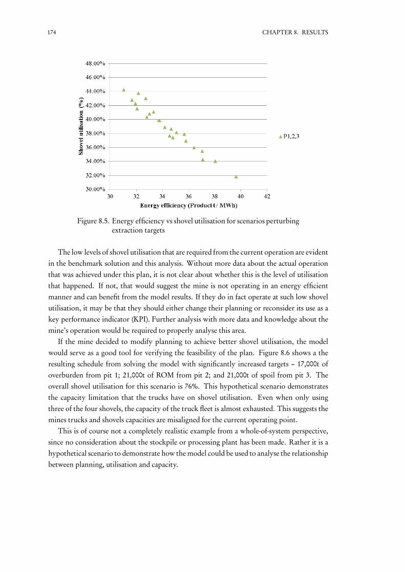
174 CHAPTER 8. RESULTS
Figure 8.5. Energy efficiency vs shovel utilisation for scenarios perturbingextraction targets
The low levels of shovel utilisation that are required from the current operation are evidentin the benchmark solution and this analysis. Without more data about the actual operationthat was achieved under this plan, it is not clear about whether this is the level of utilisationthat happened. If not, that would suggest the mine is not operating in an energy efficientmanner and can benefit from the model results. If they do in fact operate at such low shovelutilisation, it may be that they should either change their planning or reconsider its use as akey performance indicator (KPI). Further analysis with more data and knowledge about themine’s operation would be required to properly analyse this area.
If the mine decided to modify planning to achieve better shovel utilisation, the modelwould serve as a good tool for verifying the feasibility of the plan. Figure 8.6 shows a theresulting schedule from solving the model with significantly increased targets – 17,000t ofoverburden from pit 1; 21,000t of ROM from pit 2; and 21,000t of spoil from pit 3. Theoverall shovel utilisation for this scenario is 76%. This hypothetical scenario demonstratesthe capacity limitation that the trucks have on shovel utilisation. Even when only usingthree of the four shovels, the capacity of the truck fleet is almost exhausted. This suggests themines trucks and shovels capacities are misaligned for the current operating point.
This is of course not a completely realistic example from a whole-of-system perspective,since no consideration about the stockpile or processing plant has been made. Rather it is ahypothetical scenario to demonstrate how the model could be used to analyse the relationshipbetween planning, utilisation and capacity.

8.3 Asset usage analysis 175
Figure 8.6. Equipment schedule with higher shovel utilisation
8.3 Asset usage analysis
As mentioned in the last section, the second factor that was identified as a focus of this studyin Section 2.4 is asset usage. Here, several scenarios are analysed to demonstrate how themodel incorporates the asset usage factor.
8.3.1 Truck analysis
The methodology from Subsection 5.3.3 is used here to analyse the criticality of trucks in thebenchmark solution. By disabling each of the 12 trucks that appeared in the solution to thebenchmark solution, resolving and sorting by the increases in energy efficiency, the trucksmost critical to achieving energy efficiency can be determined. Figure 8.7 shows the resultsof the analysis. The ordering is mostly consistent with the results from this analysis on theoriginal model in Subsection 5.3.3, though there are slight differences. These are because theimproved accuracy of the scheduling formulation brings a slightly different mix of trucks intothe solution. Trucks 4 and 6 are once again two of the most critical trucks, with trucks 1 and2 joining them now. The three new trucks (5, 7 and 11) that were added into the solution withthe increased accuracy of the new formulation appear towards the bottom, alongside truck18 and 13.

176 CHAPTER 8. RESULTS
Figure 8.7. Effect of taking out each truck from benchmark solution
Another way that trucks can be analysed is by perturbing their energy consumption coef-ficient parameters. A similar methodology that was used to get the above results can beapplied to analyse the effect of improving each truck’s energy efficiency on the overall energyefficiency of the system. Figure 8.8 shows the energy efficiency gain of reducing the energyconsumption of each truck by 10%. This shows that improvement to truck 2 would resultin the biggest gain in energy efficiency, closely followed by trucks 4, 1 and 13. Reducing theenergy consumption of trucks 11, 18, 5 and 7 would result in the least improvement of overallenergy efficiency, besides making improvements to trucks that aren’t being used.

8.3 Asset usage analysis 177
Figure 8.8. Effect of taking out each truck from benchmark solution
These two methods of analysis show useful ways to study the asset usage factor. Thefirst analysis informs operators of the equipment that is most important to achieving energyefficiency for a particular plan, which can assist dispatching decisions. The second could beused to inform decisions about where the most value can be realised by maintenance thatimproves equipment efficiency.
8.3.2 Cycle time analysis
Key to the operation of the excavation and haulage subsystem and usage of its equipment isthe cycle time of trips. In this analysis, the loading times, driving times and both combinedare perturbed by ±20%. Figure 8.9 shows the impact that each of these three scenarios hason the energy efficiency of the system and the shovel utilisation. Increasing each of thesethree parameters has a principally linear impact on energy efficiency, with the relative changeto loading time having the least impact, followed by driving and, understandably, the wholecycle time.

178 CHAPTER 8. RESULTS
Figure 8.9. Energy efficiency and shovel utilisation of scenarios perturb-ing cycle time
This however, does not show the relationship on a per minute basis. For instance, anincrease of 20% for a 13 minute driving time corresponds to a 2.6 minute increase but to only0.7 minutes for the loading time. Depending on the context of the analysis it may be moreappropriate to compare the impact of changing the times by the same amount of minutesrather than the same relative change.
Table 8.5 has been compiled to show the ‘per minute’ impact on energy consumption andefficiency that each scenario results in. Average driving and cycle times have been used toweight them, based on the balance of trips that are present in the solution. This was notneeded to be done for the loading time as it is the same across all equipment.
Table 8.5. Marginal cost per kilotonne of plan target
Scenario MWh /minute (Product t /MWh) /minute
Loading time 10.51 -1.51Avg. driving time 4.96 -0.69Avg. whole cycle time 6.69 -0.99
Referring back to Figure 8.9, the shovel utilisation has a negative relationship with effi-ciency; as loading times increase and energy efficiency decreases, utilisation rises – reiteratingthe point made at the end of Section 8.2 that shovel utilisation should not be relied upon as ameasure of energy efficiency. It does not change when driving times are perturbed.
8.3.3 Truck waiting time analysis
Times where trucks wait to be loaded at the shovel is a common point of interest wheninspecting the efficiency or productivity of the truck and shovel fleet. It is a key improvement

8.3 Asset usage analysis 179
to the subsystem formulation that this study contributes. As mentioned in the benchmarkanalysis, truck waiting time only accounts for a small percent, 0.56%, of the total energyconsumption. This makes analysing it difficult when perturbing parameters and inputs, as theother analyses have been done in this chapter, since other factors have a much greater influenceon the energy consumption of the system. So to analyse its impact, 70 feasible solutions tothe benchmark instance have been recorded from 10 runs of the solution technique.
Figure 8.10 shows a correlation between truck waiting energy and overall energy effi-ciency. Lower truck waiting energy, and hence truck waiting times, are seen as more energyefficient. This indicates the relationship is being taken into account but is a relatively weakcorrelation with the energy consumption objective for the case study mine. Since truckwaiting time is often looked at as a key performance indicator (KPI) of the excavation andhaulage activity, this loose correlation suggests it may not be the best KPI for operators tofocus on when looking for energy efficiency improvements.
Figure 8.10. Energy efficiency vs truck waiting energy
8.3.4 Shovel availability analysis
The last analysis relating to the asset usage factor identifies the shovel and state most criticalto the optimal solution. To do this, a constraint that disables a shovel in a particular state wasadded to the model and solved for each combination of shovel and state. For the shovel at pit2, where ROM is being extracted, in state one, this constraint introduced conflicts with theminimum stockpile limit constraint, so the minimum stockpile limit was reduced to 18,800tonnes for this analysis.
Figure 8.11 shows the energy efficiency loss by disabling each shovel from each state of thebenchmark instance. The shovel at pit 2, where ROM is being extracted, in states three andfour, has fairly consistent energy loss across the states and has the largest impact on energyefficiency. This is due to the increased double handling required at the ROM stockpile to allow

180 CHAPTER 8. RESULTS
the processing plants to continue operating. The interactions between the various subsystemson display here is another demonstration of the benefit of integrating them all into a singlemodel. Without considering the downstream stockpile and CHPP subsystems, the real costof the shovel unavailability could not be calculated.
Figure 8.11. Energy efficiency lost from outage of each shovel in each state
The shovels at pit 1 and 2, digging overburden and spoil respectively, exhibit a more variedresult. For the first two states, the increase in energy consumption is quite minor. Thisis because the two targets do not have a direct impact on the rest of the mine and since theexcavation and haulage subsystem is operating with excess capacity, it is able to account for theloss evenly throughout the day. However, the reason behind the increased losses of the thirdand fourth state is not clear. These two states appear to exhibit a more subtle, unexpected,behaviour isolated to within the excavation and haulage subsystem. While trip numbers andshovel utilisation remain unchanged between the state 2 and 3 scenarios, the solutions for thestate 3 scenario exhibit the more truck waiting time and hence more energy consumption.The cause of this is unknown at this stage. It is also strange that it doesn’t seem to appear inthe pit 2 shovel unavailability scenarios. Detailed investigation looking into this phenomenonshould be carried out in future work to determine the cause.
This analysis also serves as a demonstration of how the maintenance aspect of asset usagecould be considered using the model. As explained in Section 2.3, asset availability is directlyimpacted by maintenance activity. Running these scenarios and similar could help assistdecisions about planned maintenance that will have the least impact on the energy efficiencyof the mine.

8.4 Remarks 181
8.4 Remarks
This chapter has revisited the case study to give practical verification of the improved integ-rated model and the solution technique that has been innovated to solve it. The model nowprovides a much more accurate solution for the case study mine’s excavation and haulagesubsystem, overcoming synchronicity issues experienced in the first run of the case study, inChapter 5. This is delivered in the form of a shovel and truck schedule, which is an originalcontribution that is significant both academically and practically. Finally, while the improvedmodel was too hard for exact solution techniques to solve for real life-sized problems, likethe case study, the solution technique developed in Chapter 7 was shown here to be able togenerate quality solutions in reasonable time.
Several scenarios have been analysed to show these outcomes. These were presented fromthe context of the two factors introduced in Section 2.4 as areas of focus when modellingoperational energy efficiency of a mine. Initially, the planning factor was analysed by extend-ing upon the initial results, using the original model presented in Subsection 5.3.2. Plannedtargets, inputs to the model, were perturbed and the resulting impact on energy consumptionand efficiency were analysed. The model behaved well across the range of instances andprovided sensible, consistent results. The benefit of the integration was on display whenanalysing the diminished returns of due to the ROM stockpile hitting its lower limit. Themarginal cost per kilotonne of each target perturbation was also presented as a compact wayof interpreting the results. Finally, a look at the impact extraction targets have on shovelutilisation suggested that shovel utilisation is not necessarily a good indicator of energy effi-ciency.
The asset usage factor was analysed in four ways. Firstly, the truck analysis introduced inSubsection 5.3.3, was used to identify the trucks that are most critical to achieve the mostoptimal benchmark solution, and how the solution improves with more efficient trucks.Secondly, a sensitivity analysis on the cycle time parameters found that the model behaves welland produces expected results. A look into truck waiting times found that, while the impact oftrucks waiting at the shovel is relatively small compared to other factors at play, a relationshipdoes exist with energy efficiency. However, the variance suggests truck waiting time is notnecessarily a good indicator of energy efficiency. Finally, scenario analysis that looked at theimpact of unavailable shovels throughout the day was conducted. This highlighted the valueof the integrated model and also uncovered some interesting behaviour when the shovel at pit2 is unavailable later in the 8 hour period. This should be the focus of further work, to discoverwhether it is a problem with the model and solution technique or a physical phenomenon atthe mine.
This chapter completes the bottom left quadrant of Figure 8.12 of the research approachdetailed in Section 1.5. The case study has been revisited with the improved model andsolution techniques, from Chapter 6 and Chapter 7 respectively. The improved model wasshown to be superior to the first iteration in practice, and the solution approach providesquality solutions in reasonable time for practical-sized problems. Chapter 9 next completesthe loop of the research approach by discussing the outcomes of the research to outline the

182 CHAPTER 8. RESULTS
opportunities that they present and concludes the thesis by revisiting the research questions,aims and hypothesis.
Figure 8.12. Role of Chapter 8 in the research approach
The content of this chapter addresses all three research questions listed in Section 1.2, listedbelow, by applying the various contributions from the thesis so far in a detailed analysis ofthe case study mine. The modelling approaches and formulation have been verified in detailwith relation to a real life example of the general problem being addressed by this thesis. Aswell as this, the solution technique’s usefulness for practical application has been validated.
1. How can the energy efficiency of mining production systems benefit from an integratedmodelling approach?
(a) Why is improving energy efficiency a concern for mining operations?
(b) How can an open-pit coal mine be considered as a production system?
(c) What factors impact the energy efficiency of a mine?
(d) What are the benefits of using a quantitative optimisation model of energy efficiency?
(e) Why take an integrated optimisation approach?
2. What integrated optimisation model of energy efficiency is appropriate for an open-pit coalmine production system?
(a) What level of detail is required of the model?
(b) Where are the main points of model complexity?

8.4 Remarks 183
(c) How general should the model be?
(d) What is an appropriate process for applying the model to a real life mine?
3. What solution techniques will be appropriate for solving the model in real-time?
(a) How hard is it to solve the developed model? Is the optimisation NP hard?
(b) Are new techniques required?
(c) What impact do any new solution techniques have on optimality and speed?


9Discussions and Conclusions
This chapter finalises the thesis by first using the case study results to discuss the opportunitiesfor providing support to operating mines for making improved decisions about energy effi-ciency. Secondly, the contributions of the research are examined from the perspective of theiracademic and practical implications. The limitations of the outcomes are then highlighted,and future work is earmarked for improving upon the contributions of the study. Finally,concluding statements assert the success of the research.
185

186 CHAPTER 9. DISCUSSIONS AND CONCLUSIONS
9.1 Opportunities
The final step of the research approach improvement loop, described in Section 1.5 and high-lighted in Figure 9.1, is to identify the opportunities that the results present, to the case studymine and the problem of open-pit coal mine energy efficiency in general. A suite of decisionsupport software tools is also proposed as a way of applying the research findings in practice.
Figure 9.1. Role of Section 9.1 in the research approach
9.1.1 Opportunities for Meandu Mine
Results using both the Chapter 4 and Chapter 6 models, presented in Chapters 5 and 8 respect-ively, demonstrated clear opportunities for supporting energy efficient decisions at MeanduMine. Using data that was readily available to the mine operators and information gatheredduring a mine visit, the application process presented in Section 3.3 was followed to createan integrated model of Meandu Mine. Using information about their current operation, abenchmark shift plan was established. Comprehensive sensitivity and scenario analysis gaveinsight into how their operators can use the model for making energy efficient decisions.
Excavation and haulage opportunities
Since the excavation and haulage subsystem represented the majority of energy consumptionand had the most detailed data, the focus of the analysis primarily centred around how itsoperation impacts the whole mine energy efficiency. At the current, benchmark, operatingpoint, a relatively high level of excess capacity appears to exist in the excavation and haulage

9.1 Opportunities 187
subsystem. Whereby to meet the planned operation, shovels were only required to operateat around 40% utilisation, and several trucks were not required.
This presents two avenues for potential opportunity. Firstly, if the mine’s actual operationis not reaching a similar level of utilisation, it is unlikely they are operating in an energyefficient way. They could therefore benefit from directly using the benchmark solutions to themodel to guide excavation and haulage subsystem operation, to achieve the extraction targetswith less energy consumption. The model provides a detailed picture of energy efficient truckand shovel activity that operators could use to aid their truck dispatching decisions. How thiscan be achieved is discussed in more detail in Subsection 9.1.2.
The second avenue for opportunity to come out of the low utilisation insight is the poten-tial for better alignment between their planning, capacity and performance measures. Thiscould benefit the mine in more ways than just energy efficiency, as equipment utilisation is akey performance indicator (KPI) used to reflect the productivity of the mine’s operation. Ifthe planned operating point can be achieved with relatively low utilisation, either planningshould increase extraction to allow operation to achieve higher utilisation or utilisation isn’tthe best KPI for operation to focus on.
Changing the extraction plan is, of course, not a trivial exercise that should be done basedon one finding, rather, this is based on many different variables outside the scope of thisresearch. However, using some simple reasoning, a case can be made to warrant furtherinvestigation. Firstly, it is important to realise that the case study mine is in a particularsituation. It only has one customer and has well known demand. Therefore, simply increasingthe overall extraction targets would only lead to an imbalance with demand and unnecessarilyhigh stockpiles. Rather, it may be beneficial to reduce the operating hours of the mine.
Currently, the excavation and haulage operates 24 hours a day, seven days a week. If thesehours were reduced and the excess capacity was employed to increase output during operatinghours, the equipment utilisation during the operating hours would increase. This wouldpotentially lead to operating cost reductions, especially if night time and weekends are moreexpensive to times to operate. The processing plant already uses this strategy by turning offon weekends. Depending on the specifics of how this would be implemented, it may notnecessarily lead to increased energy efficiency. However, scenario analysis using the modelcould be used in a cost benefit analysis to help decision makers investigate options.
On the other hand, if changes to the plan are not suitable options, these results maysuggest that utilisation isn’t the best KPI for operators of this mine to target. From an energyefficiency perspective, this is supported by the results in Section 8.2 and Subsection 8.3.2,which gave examples of where energy efficiency and shovel utilisation can have a negativerelationship. From a broader perspective, focusing on improving the low utilisation KPI maylead the operators to deviate from the medium and long term plans. Perhaps a ‘plan corrected’KPI could be developed to give operators a better indicator of their utilisation compared towhat utilisation is required to meet the plan. In this case, the model could be used to determinethe expected utilisation for a given plan. Using this would enable operators to see that the lowutilisation is okay, reducing the risk of them deviating from longer term plans and increasing

188 CHAPTER 9. DISCUSSIONS AND CONCLUSIONS
the importance of other KPIs that will lead to cost reductions, such as energy consumption.Subsection 8.3.3 addressed another KPI that the mine uses to measure the performance of
the excavation and haulage subsystem - truck waiting time. While this KPI isn’t necessarilyrelated to the excess capacity discussed so far, the results demonstrated that it too may not bethe best measure of energy efficiency. As expected, a positive relationship to energy efficiencywas demonstrated, however, the variance was quite high. This indicates that other variableshave a much higher impact on energy efficiency. Focusing on truck waiting time is thereforenot entirely appropriate for making energy efficiency decisions. It is no doubt a useful indic-ator of other important costs, but it is important for decision makers to understand the limitof its applicability. Instead, it is suggested that new KPIs be developed based on the results ofthis research and that of May et al. (2015).
As well as these avenues for opportunity, there is also the possibility that the data providedby the mine is erroneously misrepresenting the mine’s capacity and current operating point.Therefore, more data about their current plans and actual operation would be required toexclude this possibility.
Whole-of-mine opportunities
As well as the opportunities contained within the excavation and haulage subsystem, severalopportunities present themselves for using the model to aid wider decisions about the wholemine. In Section 8.2, the current operating point of the whole mine was shown to havea degree of flexibility. Increasing all extraction and demand targets across the mine by thesame factor did not affect energy efficiency significantly. This means the mine is in a goodposition to increase its workload to accommodate for disturbances, without impacting energyefficiency. For example, if rain impacted operation for a day, extra work for the remainingworkload for the next couple of days to ‘catch up’ with planned targets could be done withoutadverse impact on energy efficiency.
Another opportunity identified for the mine is to introduce grade control into their opera-tion. At the moment, they consider all ROM coal equally and process it into a single productgrade. The general model presented in this thesis has been designed to account for varioustypes of ROM and product grades. By modifying the current model of the mine to includemore material grades, the impact of grade control on energy efficiency could be analysed aswell as the impact on the mine’s operation.
Taking this idea further and considering downstream from the mine, the power stationit provides product coal to could also be included in the model, to achieve an even widerlevel of system integration. Since the mine only services the power station, operators of thetwo systems are in a very good position to align their operation to get maximum value outof their interactions. Power stations are also continuous production systems, meaning theintegrated modelling framework and application process developed in this research wouldsuit this endeavour well.
By formulating a power station subsystem module and connecting it to the existing model,a number of scenarios could be analysed. For example, various demand profiles for product

9.1 Opportunities 189
coal coming out of the wash plant could be analysed to see if less double handling at the powerstation stockpile could be achieved. This could be used to further analyse the previouslymentioned opportunity to operate the excavation and haulage subsystem at reduced hours toincrease its utilisation, and synchronise its workload with the demand profile.
Another example would be to analyse the impact that more grades of product would haveon the efficiency of the power station. For instance, using lower quality coal when the powerstation is operating at low loads and higher quality coal at high loads could lead to moreoverall efficiency of the power station. There is currently legacy wash plant bypass that waspreviously used for high quality coal and didn’t need to be washed, but it is not used anymore.It may be that crushed ROM coal could use this bypass to go straight to the power stationwhen the power station is at low loads, removing the cost of washing.
As well as this, several possibilities for other improvements to various parts of the minewere brought up in informal discussions with operators during a site visit. Large scale strategicinvestment options were discussed as potential areas of investment. This model could be usedto analyse each option’s impact on energy efficiency compared to the current operation of themine. For instance, an obvious double handling cost is the crushed ROM stockpile betweenthe crusher and wash plant. Investing to change this to be a more efficient transfer betweensubsystems, such as a surge bin, could lead to energy efficiency improvements when the twosubsystems are both in operation. Decision makers would be able to use the model to conductcost benefit analysis around such investment options.
9.1.2 Opportunities for open-pit coal mines
Rather than cutting the problem down to only model the specifics of the case study mine, thepractical applicability of the research to other mines has been a focus. Therefore, beyond theopportunities that this thesis presents to the case study mine, there are many opportunitiesfor addressing the problem of open-pit coal mine energy efficiency in general. These are theease of applying the methods to new mines; the ability to quantify factors that impact energyefficiency; how various levels of decision making can be assisted; and how the model can bedeveloped into a decision support software tool.
Efficient modelling of operating mines
The modelling framework, application process and general integrated model presented in thisthesis have all been designed to reduce the upfront cost of modelling new mines. This wasdemonstrated using the case study mine. With existing, readily available data provided bythe operators, an integrated model of the main operations of the mine was able to be createdwith the integrated modelling framework, using the four subsystem module formulations.This was done with the assistance of the model application process, which proved to bean effective process for efficiently translating from the mine’s ‘problem domain’ into themodelling ‘solution domain’.
This is an important outcome as it means creating models of new operations does notrequire a massive upfront effort in terms of cost or time. Getting value from the model sooner

190 CHAPTER 9. DISCUSSIONS AND CONCLUSIONS
at a lower cost means a shorter payback period on initial investment. This is a design featureof the research outcomes to help ensure their practical viability. Lower initial investment anda shorter payback period are encouraging traits for companies that are considering applyingthe model to their operations.
The model design also means that mines can use their existing data to form a baseline oftheir current performance, to measure the progress of improvements. The approach allowsfor scaling up when more resources and data are available, to make a higher resolution, moreaccurate model as required. Once again, this reduces the initial investment and therefore thepayback period. It also increases the likelihood that any given mine can apply the model, asmines with less available data should still be able to get a model of their operation running.Once the model is running on existing data, any investment that improves the model accuracycan then be directly compared to the previous versions of the model, to help mines see wheretheir efforts may be best spent.
In particular, other open-pit coal mines that solely service a power station are in a verygood position to benefit from this research. While the modelling is based around a generalopen-pit coal mine, the detailed analysis of its application and resulting opportunities werecentred on the case study mine. This places similar mines in a good position to apply themodel with a higher degree of certainty that the concepts will carry over to their operationand provide them valuable results.
Analysing factors impacting energy efficiency
As Thiede (2012) suggests, energy efficiency modelling and analysis should aim to considermany factors that influence a production system. The modelling effort in this thesis focusedon asset usage and planning factors. Their impact on the case study mine was analysed inChapter 5 and 8. Other factors listed in Section 2.3 can also be analysed using the model,using scenario and sensitivity analysis. An example of this is the investigation of the assetownership factor also conducted on the case study mine. By using these factors to classifyand describe the application of the model, a deeper analysis of the energy efficiency can beconducted.
Framing analysis around these factors is an effective way of applying the learnings of alarge body of production system literature to practical application of the model. Rather thanlooking at results as discrete outputs that only apply to the mine being modelled, relating theresults back to these factors allows for deeper insights.
For example, the results in Subsection 8.3.1 provide indication of which trucks are mostcritical in achieving energy efficiency for the current operation. However, when conductinga deeper investigation into these results, it can be seen that a number of factors are at play.The impact of asset usage for each truck is being quantified for operators to use to prioritisetheir decisions around keeping the most critical trucks available and working. Maintenanceactivity, which falls under the asset usage and ownership factors, can also use the results toweigh up the impact of temporarily removing each truck and improving its efficiency. Allthe while, these results are taking into consideration the current planned operation, another

9.1 Opportunities 191
important factor.Detailed scenario and sensitivity analysis can be performed to separate and quantify the
influence of each of these factors on energy efficiency. This is a useful method of identifyingopportunities to improve energy efficiency. By using to model to quantify the influenceof each factor, companies can see where their efforts may be best spent to make overallimprovements to the whole-of-mine energy efficiency. This type of analysis is recommendedin the EEX, formally EEO, program that formed part of the motivation for this researchDepartment Resources Energy and Tourism (2010).
Quantifying the influence of the factors is also important when trying to compare themine’s operation to other mines or a best practice. Mines are highly exposed to externalvariables, such as geography, geology and weather, as mentioned in Section 2.2 and 2.3. Thismakes it harder to compare one mine against another, which can become a barrier that stopsmines from improvement towards best practice. However, being able to quantify then removethe influences of such external, uncontrollable factors, allows mines to put themselves on amore even playing field, to compare against one another or a best practice. This can be usefulfor identifying opportunities and measuring improvements.
Decision making levels
Central to the primary aim of this study was to present opportunities to assist decision mak-ing. Considering energy efficiency at all levels of decision making – operational, tactical andstrategic – is a key recommendation of Bunse et al. (2010). Though the model is formulatedaround operational decision variables, by performing different types of scenario and sens-itivity analysis, the model can be used to aid any of these decision making levels. In fact,the ability to use an operational model to aid medium to long-term decision making is animportant element of this opportunity. Being able to use an accurate model of the mine’soperation fit using recent data of actual operation supports better decision making. Ratherthan analysing medium to long-term decisions using only historical, design or theoretical data,this methodology enables decision makers to analyse the effect of their decisions on current,actual operation. Figure 9.2 gives examples of how the operational model can be applied tosupport the three levels of decision making mentioned above.

192 CHAPTER 9. DISCUSSIONS AND CONCLUSIONS
Figure 9.2. Examples of how model can aid different decision levels
Operational decisions, such as subsystem workload and equipment allocation, are the de-cision variables of the optimisation model. This means that solving the model on the currentoperation provides a detailed output about the most optimal way to meet planned targets,especially since the model is quick enough to run frequently as new information is gathered.For example, at the start of a shift, mine operators can enter the targets, solve the modeland get an idea about the activity required by each subsystem throughout the shift. Thiscould then be rerun when new information is available, such as equipment failure or otherunexpected events, to give a new result to follow to meet the planned targets. This wouldhelp operators stick to the plan in an energy efficient manner, using quantified justificationbased on the current operation, rather than theoretic or design information.
The results of the model can also be used to improve communication between operators ofdifferent subsystems and shifts. Because it is an integrated, whole-of-mine model, operatorscan use the model output to see how their subsystem is working as a part of the wider system.It can be used by operators to communicate with each other based on quantified details fromthe same model, rather than their own silo optimisations. Likewise, the results can be usedfor communication between the operators of two adjacent shifts. The results give a detailed,quantified, picture of optimal activity for each shift, irrespective of operator’s preferences thatcould be used to promote more consistent operation.
Aside from these operational decisions, medium-term decision support is also possible, asdemonstrated by various scenario analyses presented in the results. Planning decisions usuallymade at a tactical level are the input to the model. The results showed significant opportunityfor analysing planning options with respect to energy efficiency by way of scenario analysis.During the planning stages, the model could be run on proposed plans to see the model’sresulting energy consumption. This could be used to help make plans that use less energyconsumption.
Other medium-term decision making can also be aided using the model. Scenario analysis

9.1 Opportunities 193
looking at decisions around equipment availability, efficiency and other parameters of themodel could be used to support relevant tactical decisions. Along with these, the aforemen-tioned asset ownership decisions are usually considered at a tactical level on mines.
While it was not analysed in the results chapter, the model also has potential for being usedto aid long term, strategic level, decision making. Major changes to the structure or operationof the mine, such as a new processing plant or alternate demand agreements, would benefitfrom a detailed, accurate model of the mine’s current operation. The extensibility of themodelling framework would become useful for taking the model of the current operationand modifying it to reflect the proposed changes. Accurate and up-to-date benchmarking andcost benefit analysis could then be carried out between the two models.
As a decision support software tool
Development of a software tool is proposed to deliver the aforementioned opportunities todecision makers. It is intended that the software is designed to make a positive influence onhuman and organisational factors, described in Section 2.3, for improving energy efficiency(Cagno et al., 2013). Since there is a broad range of opportunities for many different decisionmakers across a wide variety of mines, this may be delivered in a variety of different forms.The model application process presented in Section 3.3, represented below in Figure 9.3, canbe used to help guide this discussion.
Figure 9.3. Examples of how model can aid different decision levels

194 CHAPTER 9. DISCUSSIONS AND CONCLUSIONS
Before the general integrated model contributed by this thesis can be used for decisionsupport at a mine, it must first be applied to the mine in question. This is represented by thetop half of the application process in Figure 9.3. The first piece of software proposed here isa tool that allows mine personnel, or ‘problem domain experts’, to fit the general integratedmodel to their operation; this will be referred to as ‘MineModeller’.
Once the general integrated model has been applied to the mine being modelled, it is readyto be used for decision support; this is represented in the bottom half of the applicationprocess in Figure 9.3. Extending upon the discussion from the previous section looking athow to aid different decision levels, three conceptual decision support software tools areproposed; a tool to aid operators, ShiftDashboard; a tool to aid planners, EEPlanner; anda ‘what-if’ scenario tool, EEWhatIf.
MineModellerA key feature that enables the problem domain experts to apply the model, briefly touched
on in Section 3.3, is the concept of a subsystem library. Having a library of generalisedsubsystem models, currently made up of the four subsystems studied in this thesis, allows fora flowsheet style, ‘drag and drop’, graphical user interface (GUI) that problem domain expertscan interact with, to build the layout of their mine with no modelling expertise required. Thisis the type of user interface proposed for MineModeller, shown in Figure 9.4. This takes careof the ‘Outline process flow of system’, ‘Align process flow with existing library of subsystemmodules’ and ‘Apply information to integrated model’ steps in the application process.
Figure 9.4. MineModeller GUI wireframe
For cases when systems on the mine cannot be represented using one of the generic subsys-tems in the library, the separation between ‘problem domain’, grey, and ‘solution domain’,
9.1 Opportunities 195
purple, tasks in the application process, Figure 9.3, becomes important. In these cases, a‘solution domain expert’, such as an OR modelling consultant, is required to work withthe mine to formulate the new subsystem. Once the new subsystem module formulationis finished and tested, the modeller consultant can then add it back into the module libraryto allow the users of MineModeller to continue their work.
Once the layout and process flow of mine is configured with the flowsheet interface shownin Figure 9.4, custom forms for each subsystem instance that the user includes in their minemodel are required. The various sets and parameters from the mathematical formulation ofthe subsystems, detailed in Chapter 4, would have to be translated into an appropriate GUIform for users to enter the relevant data. This is represented as the ‘Enter subsystem parametervalues’ step in the application process.
After using MineModeller to complete these steps, the mine’s operation has successfullybeen translated into a form ready to be loaded onto the model formulation, have a productiontarget task set and solved. The remaining software tools proposed here illustrate how this canbe done to achieve three different types of decision support.
ShiftDashboardThis tool is designed to achieve the opportunities for decision support at the operational
level, mentioned previously. The core concept behind the tool is to present the model’soptimal solution along with what is actually happening at the mine. Operators can useit to quickly see how well they are following the result of the model. They can use thatinformation to quantify the impact that their decisions or unexpected disturbances have hadon energy efficiency, and use it to make more energy efficient decisions. Depending onthe mine using it, the ShiftDashboard may be customised to suit the user requirements andavailability of operational data. Here, it is assumed that the mine has detailed data about thecurrent operation that can be fed into the tool in near real-time. In this scenario, the modelis re-solved with the updated data, also in near real-time, to update the optimal plan as moredata becomes available.
First of all, to solve the models created using MineModeller for a shift, the planned targetsfor that shift must be entered. This is represented by the ‘Enter shift production targets’ stepof the application process. An example GUI for entering or modifying the shift productiontargets is shown in Figure 9.5. These could be programmatically fed into the tool directlyfrom the planning software that the mine uses. This could also be used half way through ashift to update the plan and get a new result from the model. For example, after an unexpecteddisturbance, an operator may decide to increase or decrease a given production target.

196 CHAPTER 9. DISCUSSIONS AND CONCLUSIONS
Figure 9.5. ShiftDashboard target input panel wireframe
These targets can also be selected from a library of different types that correspond to tasksin the model. The terms ‘target’ and ‘task’ are kept separate here to distinguish that a target isin the problem domain, while a task is in the solution domain. At the moment, in the formu-lation, there is only a single type of task. This is a constraint requiring a given connection tohave a total mass transferred of a particular grade between a minimum and maximum amountduring specified states. This translates into a production target that specifies the minimumand maximum mass required of a particular grade between two times. If a different typeof target/task pair is required, a solution domain expert is required. This would happen in asimilar way to that in which the MineModeller deals with new subsystems. Once the solutiondomain expert has created the new task in the formulation and integrated it as a target backinto the software, the user can continue entering their shift.
Once shift targets are entered, they are loaded into the model as tasks and the modelis solved, using the Chapter 7 solution technique, and results are presented alongside theoperational data in the form of a hierarchical dashboard. The dashboard has a main overviewscreen, shown in Figure 9.6, that gives a summary of the energy consumption, production and‘health’ of each subsystem. The health is a traffic light indicator that allows users to quicklysee where deviations between plan and actual are occurring. The dashboard can be configuredto show more detail in areas that require more attention, for example, the excavation andhaulage subsystem. It is a screen that would be of particular interest to operators or minemanagers that are concerned with the whole-of-mine operation.

9.1 Opportunities 197
Figure 9.6. ShiftDashboard mine overview wireframe
In the example overview dashboard shown in Figure 9.6, there is an issue with the extrac-tion and ROM stockpile subsystems. The extraction subsystem is red because it has a majorchange to the plan; it is currently only extracting 200t/h of ROM from Pit 1. The stockpile ismarked as yellow, indicating a minor issue; this is because, while there is no current probleminside the stockpile, due to the lower than expected output from the extraction subsystem,the stockpile level is expected to reach minimum, safety level later in the day.
As previously mentioned, the dashboard is hierarchical, meaning users can ‘drill down’to subsystem dashboard levels that display more detail. By clicking on a subsystem in theoverview, the user is taken to a dashboard for that subsystem. Continuing on with thisexample, the excavation and haulage subsystem dashboard is shown in Figure 9.7. Thesesubsystem screens of the tool are where operators of the individual subsystems can get adetailed picture of their responsibilities, and a brief insight into subsystems connected totheirs.

198 CHAPTER 9. DISCUSSIONS AND CONCLUSIONS
Figure 9.7. ShiftDashboard excavation and haulage subsystem wireframe
These can be customised to suit the requirements of the user. In this example, the usercan see a number of different pieces of useful information. In the centre of the screen is themain output of the excavation and haulage subsystem formulation, the equipment schedule.Depending on the availability of real-time data, this could be merged with the actual trucklocations to show the user how far away they are from the optimal plan. Other informationrelevant to the operators can also be seen, such as the shovel utilisations and average truckwaiting times. More advanced output from running automated scenario or sensitivity on themodel can be displayed, for instance the energy efficiency truck criticality, using the methodpresented in Subsection 8.3.1.
EEPlannerThe next tool is designed to help planners make more energy efficient plans. It reflects an
example of the opportunity to support medium term, tactical level decision makers. It is notas centred around a GUI, rather, it is how software can be used to integrate the model withexisting planning processes and software used at the mine. Figure 9.8 exhibits the existingplanning systems and data used at the mine and the proposed role of EEPlanner, highlightedin green.

9.1 Opportunities 199
Figure 9.8. EEPlanner workflow diagram
The EEPlanner will be implemented to solve the model using the output of the currentplanning software as the planner creates it. It may solve one or several shifts depending on theoutput of the planning software. When solving several shift plans, they will be solved in seriesto correctly pass certain variables, such as the stockpile levels, between the shifts. Solving theshift(s) using the model validates that the shift can be achieved and gives an optimised energyefficiency achievable for that plan.
The EEPlanner will also use recent data about the operation of the mine, if available, suchas equipment efficiency and loading times. This means the model is solved with an up todate picture of the mine’s operation to ensure the result accuracy. By bringing this data intothe planning phase, the tool helps planners make decisions based on recent operation ratherthan outdated or theoretical data. This follows the theory of the Plan-Do-Check-Act cycle(Walton, 1988).
The model results can then be delivered back to the user in a number of ways. Firstly,a report can be generated. This would contain high level information about the subsystemworkload and energy consumption required to meet the plan. Sensitivity analysis, similar tothat presented in Section 8.2, could also be generated and included in the report to give usersan idea about what changes could be made to improve the energy efficiency of the plan.
The ShiftDashboard GUI could also be used to present the results of the EEPlanner tothe user. This shows the planner exactly what their plan will look like to operators. Havingplanners see their shifts in this light promotes a deeper understanding of how their outputsare used and the role of operators.
As well as these two options for presenting the EEPlanner results, the third is to publishthe results back into the planning software. Depending on what type of integration with theplanning software is possible, this could be done by directly feeding the detailed results backto the software for it to process, or by feeding the reports back into the planning software.
EEWhatIf

200 CHAPTER 9. DISCUSSIONS AND CONCLUSIONS
The final tool presents opportunities to medium to long-term, or tactical to strategic,decision makers, typically managers, for measuring the energy efficiency impact of decisionsthey are considering. As with the EEPlanner, the core of the EEWhatIf tool is not a newGUI. Rather, it is a hybrid, or ‘mashup’, of the three tools already presented above, as shownin Figure 9.9. MineModeller is used to make alterations that represent the scenarios beingevaluated; EEPlanner is used to run each scenario, and the current model as a benchmark, ona set of shift plans; the results are then presented to the manager in the form of a report orthrough the ShiftDashboard GUI.
Figure 9.9. EEWhatIF workflow diagram
Scenarios are developed by the user in the MineModeller by starting with the currentmine model, altering it and saving it as a separate model. As many scenarios as necessarycan be saved out for the analysis. This allows for a wide variety of possible scenarios to suitmany different decisions. For example, tactical decisions around asset procurement couldbe developed as scenarios that replace or add additional equipment pieces into the model.Strategic scenarios about major changes to the mine can also be created, for example, theinclusion of a new pit.
Once the scenarios have been developed, they are each evaluated with the model usingthe EEPlanner and a set of shift plans. Depending on the questions at hand, any set of shiftplans can be used to conduct this analysis. For example, historical plans could be used if

9.2 Contributions and implications 201
the decision maker wants to see the potential impact that scenarios could have had on pastoperation; current plans to see how the scenarios will impact the immediate operation; andfuture plans for the impact on longer term operating conditions of the mine.
As explained above, the EEPlanner can provide a more accurate result when using actualoperating data, once again supporting users to follow the Plan-Do-Check-Act cycle (Walton,1988). However, of course, data changed specifically for the scenarios is not to be overwrittenby the recent data when running EEPlanner. As well as this, if historical shift plans are beingused, data from when the shift plans were used may be appropriate for solving the model.
After the scenarios are run in the EEPlanner, the results are collated into reports thatgive the user an overview of the energy efficiency and subsystem workload of each scenario.The information in the reports can be used to compare against other measures related to thedecision at hand, such as cost. The ShiftDashboard GUI can also be used to look at the resultof each scenario in detail. It may be that the results warrant further investigation; in this casethe process is followed again with more scenarios or different shift plans.
9.2 Contributions and implications
Throughout this thesis, the remarks sections, 2.7, 3.4, 4.3, 5.4, 6.3, 7.3 and 8.4, detailed howthe research approach as described in Section 1.5 and seen in Figure 9.10, was followed toaddress the research questions listed in Section 1.2. By following the approach and addressingthese questions, the thesis has successfully yielded a number of original, significant contribu-tions to knowledge. Broadly defined, these are listed below and numbered on Figure 9.10.
1. The abstraction of mining systems as open continuous flow production systems, usedto draw upon advanced production system literature.
2. The framework for formulating integrated models of continuous production systemsand process for applying them to operating systems.
3. The integrated MILP formulation of the open-pit coal mine energy efficiency problemdeveloped using the framework.
4. The solution technique innovated to overcome complexity issues with the shovel andtruck scheduling component of the integrated model.

202 CHAPTER 9. DISCUSSIONS AND CONCLUSIONS
Figure 9.10. Contributions delivered using research approach
In this section, the academic and practical implications of the contributions are discussed,along with an assessment of how they have been used to confirm the hypotheses.
9.2.1 Production system abstraction
Since there is an apparent lack of operations research literature looking at the integrated,operational energy efficiency modelling of mining systems, the mining system was abstractedto the more general field of production systems. This abstraction has been made, with success,in some recent literature (Everett, 2007; Jiu et al., 2013; Zuñiga et al., 2015) but is still in itsinfancy, relative to the broad range of advanced production system literature that miningmay be able to benefit from. It has also not, until now, been formally applied to the specificproblem of operational energy efficiency. The contribution is shown in the top left quadrantof the research approach in Figure 9.10. The abstraction and its implications are described indetail throughout Chapter 2.
Section 2.2 described the abstraction by first defining different types of production sys-tems. It then goes on to explain how a mining system can be considered as an open continuousflow production system. Once this is explained, the remaining sections of Chapter 2 employit to form a sound basis for the rest of the work carried out for the thesis.
Section 2.3 used production system literature to build a catalogue of seven key factorsthat impact energy efficiency; asset ownership; asset usage; human; organisational; energyprovision; planning; and external. Section 2.4 then looked at operational models in miningliterature. The factors were used as a way of including models that did not necessarily consider

9.2 Contributions and implications 203
energy efficiency in the review. The review found the two most important factors to considerwhen formulating an operation model, asset usage and planning. The operational miningmodels were then reviewed to find appropriate techniques for modelling each subsystem, andthe lack of integrated models that focus on energy efficiency was identified.
Production system literature was also drawn upon in Section 2.5. Integrated modelling,material flow connections and MILP formulations were each found to be popular approachesused in relevant production system literature (Ellis et al., 2010; Viere et al., 2011; Zülch et al.,2002). This justifies the modelling approach taken for this research. Section 2.6 also usedproduction system literature to gather a broad range of literature with complex models andreviewed the solution techniques required to solve them. In particular, cooperative hybridmetaheuristics were focused on (Georgiev & Atanassov, 2014; Malek, 2009; Michalewiczet al., 2006; Talbi, 2002). The results of the review have justified the solution techniquedeveloped in this research.
Two primary academic implications come out of this contribution. Firstly, the compre-hensive literature review presented in Chapter 2 has given a strong foundation for future worklooking at the energy efficiency of mining systems, particularly at an operational, integratedoptimisation model level, which was lacking in the current literature. Secondly, consideringa mining system as a production system was shown to be an effective way to leverage a largebody of research to fill gaps in mining literature. This procedure could be replicated to addressother mining system issues; for instance, maintenance planning using operational models wasidentified, in SubSection 2.4.6, as a potential gap in mining literature that could benefit fromthe application of existing production system literature.
Taking approaches from production systems and applying them to mining systems can alsohave direct practical implications. Without the need for further research, this procedure couldbe used to take best practice processes and policies from other similar production systemsand apply them to mining problems. While this is likely to have already been done in theindustry, being successful in competitive global markets requires continuous improvement ofoperational procedures, which are much more developed in other production systems suchas manufacturing.
The approach could also be useful for other industries. For example, elements of agricul-ture, the other Australian industry that experienced energy intensity increases between 1976-77 and 2006-07 (Australian Bureau of Statistics, 2010b), could be considered as a continuousproduction system. Using this abstraction, the same procedure could be used for applyingmethods from the general production system literature, for making theoretical and practicaladvances in the agriculture field.
9.2.2 Modelling framework
The second contribution of the thesis is the original modelling framework for developinggeneral, integrated formulations of continuous production systems, and the process for effi-ciently applying the models to operating production systems. This is represented as the widerregion in the top right quadrant of Figure 9.10 and was presented in Chapter 3.

204 CHAPTER 9. DISCUSSIONS AND CONCLUSIONS
Section 3.1 describes the conceptual framework in detail. The framework works by divid-ing a continuous production system into subsystem ‘modules’ with material flow connectionsbetween them. The idea is to decouple the subsystem formulations so that they can be verydifferent in nature, to best reflect their respective operations. A time dimension, described as‘operating states’, exists at the whole-of-system level of formulation to allow for changing op-erating conditions through an optimisation, and ensure synchronicity between subsystems.States can be different lengths depending on the required resolution of decision making. Theinputs to the integrated model are ‘tasks’ that describe what work is required by the systemas a whole. Solving the model will determine the operation required to best achieve thesetargets.
Section 3.2 then goes into more detail about the requirements of subsystem module for-mulations. The main requirement of a subsystem formulation is that it has material flowconnection points, so that it can be connected to other subsystems. Subsystem module for-mulations are also responsible for constraining the material flowing in and out of them. Thisis an important feature as it means the whole-of-system level of the integrated formulationdoes not need to be aware of the specific operation of the subsystems. They are also requiredto provide an objective value, in this case energy consumption, to be included in the whole-of-system objective.
In order to apply this framework to actual production systems, a model application processwas also designed. This is presented in Section 3.3. It describes the steps required to gather ap-propriate data about the operation of the system; define the problem as a system of connectedsubsystems; use existing subsystem module formulations or formulate new ones to create theintegrated model of the problem; apply the gathered data to model parameters; set up the tasksrequired to be done by the system; and solve the model for analysis of the results. This provedto be useful not only for applying the model to the case study, in Section 5.1, but for exploringopportunities to build a decision support software tool, explained in Subsection 9.1.2.
The academic implications of these contributions are far reaching. While the frameworkand application process have been used in this study to model the energy efficiency to anopen-pit coal mine, they have been designed to apply to continuous flow production systemsin general. They have been designed to allow for other objective values, to be applied to otherareas of mining, or for application to any other production system that can be represented by anumber of subsystems connected by material flow. In particular, the framework could be veryuseful for taking existing state-of-the-art subsystem formulations from literature, integratingthem, without the need for significant reformulation, and efficiently applying them to real-lifecase studies.
From a practical perspective, the modelling framework and application process promotemore efficient, lower cost modelling, allowing for a shorter payback period once the model isrunning and generating value. This was expanded upon in Subsection 9.1.2. They have beendesigned to enable the creation of models from a relatively small data set and scale up if moredata is available. The reusability of subsystem modules is also important for being able torapidly apply the framework to new systems. The process has also been designed to separate
9.2 Contributions and implications 205
the responsibilities of problem domain experts from modelling experts, so more of the workcan be done by the problem domain expert, also explored in Subsection 9.1.2.
9.2.3 Integrated model
Using the aforementioned modelling framework, two integrated models of open-pit coal mineenergy efficiency were presented that represent several contributions. The first is presentedin Chapter 4 and an improved formulation is presented in Chapter 6. The modelling done inthese two chapters is represented by the inner section of the top right quadrant of the researchapproach in Figure 9.10.
Chapter 4 presented an integrated model formulation using four common subsystemspresent in open-pit coal mines, excavation and haulage; processing plant; stockpile; and beltconveyor. This model is an original and substantial contribution as it combines operationalmodels for subsystems across a whole mine into a single integrated model.
These subsystems were designed to reflect the availability of data at the case study mine andmodels from existing recent mining literature. The detail of the processing plant, stockpileand conveyor belt modules were limited due to data availability constraints. However, theywere successfully modelled as general subsystems based on recent literature (Hanoun et al.,2013; Middelberg et al., 2009; Ta et al., 2005) that should be portable to many other open-pitcoal mines.
The availability of data for the excavation and haulage subsystem was much better andtherefore afforded a more detailed model. The Chapter 4 formulation of the excavation andhaulage subsystem was based around using a similar allocation decision variable to that usedin the majority of recent operational models of truck activity (Mena et al., 2013; Sahoo et al.,2014; Souza et al., 2010; Ta et al., 2013). The formulation also extended upon these othermodels by including a time dimension to allow for changing operating conditions throughoutthe optimisation period. While the Chapter 4 formulation was shown to provide sensible andvaluable results on the case study, a number of limitations were found relating to the usage ofequipment allocation to model the operation of the excavation and haulage subsystem.
To rectify these issues, Chapter 6 revisited the excavation and haulage formulation. Theimproved excavation and haulage formulation included truck and shovel interactions and tripsequencing so that the equipment operation could be more accurately accounted for. Thenew formulation is similar to that of Chang et al. (2015), the only other truck schedulingseen in literature. However, the Chapter 6 formulation is distinct from Chang et al. (2015) asit minimises energy consumption, integrates with other subsystems at a material flow leveland allows for changing operating states throughout the optimisation period. The improvedaccuracy came at a cost however. This model was shown to be NP-hard and demonstrated tobe intractable for practical sized problems.
The two models are both useful contributions to academia. While the first has limitations,it is the first of its kind to integrate all four subsystems. It is able to be solved quickly withcommercial solvers and, despite accuracy issues, still provide sensible results. Depending onthe problem at hand, the accuracy of this model may be more than enough. Meanwhile, the

206 CHAPTER 9. DISCUSSIONS AND CONCLUSIONS
improved excavation and haulage subsystem module formulation represents the state-of-the-art in modelling for that subsystem.
They also have the ability to provide valuable implications in practice. The integratednature of them means they can be used to help mine operators work toward system wideoptimums rather than suboptimal solutions from silo optimisations. Being able to have anoperational model of a running mine fit with up-to-date data means the models can provideprecise decision support relevant to the mine’s current operation, rather than design, theor-etical or historical data.
The speed of the first model means it could be used to provide quick answers, with loweraccuracy, to users making operational decisions. The improved formulation, along with thedeveloped solution technique presented in Chapter 7 and summarised below, can then beused to provide an even greater level of accuracy to decision makers. Looking towards thefuture of mining, technological advances in autonomous shovels and trucks are expectedto provide significant economic benefits (Bellamy & Pravica, 2011). Advanced operationsresearch techniques, such as those demonstrated in this thesis, will be required for accurateand optimal scheduling of this technology.
9.2.4 Solution technique
A high level, teamwork hybridisation of a simulated annealing and tabu search was innovatedto overcome the NP-hard complexities of the Chapter 6 excavation and haulage subsystemformulation. This was presented in Chapter 7 and deals with the inner section of the bottomright quadrant of the research approach in Figure 9.10.
In order to apply the tabu search and simulated annealing metaheuristics to the complexformulation, several elements were innovated. Subsection 7.1.1 described the solution rep-resentation that significantly reduces the search space of the model. Subsection 7.1.2 thendetailed seven neighbourhoods around this solution. Since the solution representation onlyrepresents the excavation and haulage subsystem, it was noted that special consideration mustbe made for two of these neighbourhoods as they can cause infeasibilities in other subsystems.
Several algorithms were then presented in Subsection 7.1.3. To check solutions that aregenerated from the aforementioned neighbourhoods that may cause infeasibilities on othersubsystems, MILPVALIDATE was designed. This solves the Chapter 4 MILP with alloc-ation set based on the candidate solution to determine if any constraints of other subsys-tems have been violated. For solutions generated using the other five moves, the ISFEAS-IBLESEQUENCE algorithm ensures the solution represents enough work from the subsys-tem. The SCHEDULESEQUENCE algorithm is developed to convert a sequence into aschedule. The schedule is then used by EHENERGYCONSUMPTION and F to calculatethe energy consumption of the subsystem and whole-mine, respectively.
Subsection 7.1.4 then presented is the constructive heuristic that builds the initial feasiblesolution required by the metaheuristics. This also uses the Chapter 4 MILP to ensure thesolution is feasible for the whole integrated model and for truck recommendations whenbuilding the sequence. It represents a low level, relay hybridisation between the heuristic and

9.2 Contributions and implications 207
exact method solving the MILP, as per the Talbi (2002) taxonomy.The tabu search and simulated annealing algorithms are then presented in Subsections 7.1.5
and 7.1.6, respectively. They both follow relatively standard algorithm flows. However, therequirement to use the algorithm to check certain solutions makes them low level, teamworkhybridisations between the heuristic and exact method solving the MILP, as per the Talbi(2002) taxonomy.
Drawing upon the concepts and techniques reviewed in Section 2.6 (Georgiev & Atanas-sov, 2014; Malek, 2009; Michalewicz et al., 2006; Talbi, 2002), the two metaheuristics werehybridised. A novel approach that utilised good practice software architecture theory and im-plementation resulted in a high level, teamwork hybrid metaheuristic, as per the Talbi (2002)taxonomy. With relatively minimal changes required to their algorithm flow, the publisher-subscriber software design pattern (Gamma et al., 1994) was used to facilitate communicationbetween the metaheuristics running in parallel. They were implemented to communicateasynchronously via ØMQ, an open source, lightweight message queue framework (Hintjens,2013). This enabled cooperative behaviour between the metaheuristics that resulted in im-proved solutions without a large increase in computation time.
Using hypothetical problem instances and case study problem instances, in Section 7.2,comprehensive computational analysis was conducted on the solution technique. Firstly, thesolution technique was shown to find optimal results to the small problems for which CPLEXcould find solutions to the Chapter 6 MILP. It was then demonstrated to curb the complexityissues that CPLEX faces, to provide good quality solutions in reasonable time for medium-to-large-sized problems. Finally, the value of the hybrid technique over the two metaheuristicson their own was demonstrated. It consistently provided the most optimal result, without agreat deal of extra computation required.
From an academic perspective, the developed solution technique demonstrates how toovercome the complexity issues with the scheduling formulation of the excavation andhaulage subsystem. It also serves as a good example for dealing with localised complexitiesin integrated models, while still ensuring the feasibility of the overall integrated model. Thehybrid tabu search and simulated annealing technique also demonstrated a novel example ofhow software architecture practices can aid the efficient development of good quality solutiontechniques.
Practically, this contribution was shown to enable the complex but accurate Chapter 6integrated model to be solved for real problems. This means the various benefits of themodel can be realised on operating mines to provide good quality solutions. The speed of thesolution technique also means the model can be solved for a number of different applications,including in an operational setting, as described in Subsection 9.1.2.
9.2.5 Confirmation of hypothesis
The contributions throughout the thesis, summarised throughout this section, have been usedto comprehensively test the hypotheses outlined in Section 1.4 and listed below. The vastarray of opportunities, detailed in Section 9.1, for the case study mine and the problem in

208 CHAPTER 9. DISCUSSIONS AND CONCLUSIONS
general, confirms each of the hypotheses.
1. Mining operations can benefit from modelling techniques commonly used in productionsystems literature.
The production system abstraction is a critical contribution for forming the strong re-search foundation presented in Chapter 2. By using this foundation, the research has been ableto apply the techniques used in advanced production system literature to the mining problemat hand. The resulting opportunities for making an improvement to open-pit coal mineenergy efficiency demonstrate that this was a successful endeavour, confirming hypothesis1.
2. Integrated modelling is an effective approach to modelling the energy efficiency of miningproduction system.
3. Mixed Integer Linear Programming (MILP) is appropriate for formulating an integratedmodel of the energy efficiency of an open-pit coal mine.
Integrated modelling is an approach that was identified and reviewed in the productionsystem literature mentioned above, as well as in mining literature, though to a lesser degree.This was reviewed in Section 2.5, where MILP was also identified as a popular and success-ful approach for formulating the integrated models. These findings formed a basis for theintegrated modelling framework contribution presented in Chapter 3 and integrated MILPformulation presented in Chapters 4 and 6. After applying these contributions to the casestudy mine, the opportunities to improve energy efficiency demonstrated the effectiveness ofthe integrated modelling and MILP formulation approaches. This confirms hypotheses 2 and3.
4. A complex model is required to accurately model the operation of an integrated open-pitcoal mine system, in particular the operation of the trucks.
Though the Chapter 4 MILP model exhibited promising results for the case study inChapter 5, detailed inspection highlighted some inaccuracies with the formulation. In par-ticular, the activity of the trucks interacting with the shovels was shown to be a problemarea. This motivated the modifications made in Chapter 6 to improve the accuracy of theexcavation and haulage subsystem. A scheduling formulation was proposed and examined toshow the accuracy was improved. The results in Chapter 8 then demonstrated the benefit ofthe improved accuracy. This confirms hypothesis 4.
5. A hybrid metaheuristic-based solution technique is able to overcome complexities in themodel to provide solutions quickly without significant loss of solution quality.
The drawback of the improved formulation presented in Chapter 6 is its NP-hard com-plexity. Practical-sized problem instances of the model cannot be solved with exact methods.To overcome this issue, various elements were innovated and detailed in Chapter 7 to be able

9.3 Limitations 209
to apply the tabu search and simulated annealing metaheuristics. These two metaheuristicswere also hybridised to allow them to cooperatively find good solutions in reasonable timeto practical-sized problems. Computational analysis in Chapters 7 and 8 demonstrated thevalue of the hybrid solution technique, confirming hypothesis 5.
6. The developed model and solution technique can be used as a decision support tool formaking more energy efficient decisions.
Finally, Section 9.1 of this chapter covered how each of the contributions can be used fordecision support. Numerous opportunities for using the model, solved with the solutiontechnique, to support decisions at the case study mine were outlined in Subsection 9.1.1,confirming hypothesis 6. Subsection 9.1.2 extended upon this to discuss how the model,solved using the solution technique, can be used to aid a decision for the problem in general.In particular, a suite of software tools were proposed to aid decision makers at operational,tactical and strategic levels.
9.3 Limitations
While the original contributions of this study have been shown to have substantial implica-tions, the approach also has a number of limitations. With respect to the modelling frame-work, the assumption that subsystems can only be connected via material flow connectionsrestricts the ability to model many interactions. This did not cause issues for this problem,and it is suggested that other continuous flow production systems should suit this restriction;it may not always work as well as it has in this study. For instance, modelling other, lesscontinuous operations at a mine, such as drilling and blasting, auxiliary systems, or trainloading, may be harder with material flow.
While the modelling framework theoretically allows for different, or more, objectives, ithas only been implemented with an energy consumption objective. This means the modelresults may have detrimental effects on other important measures of mine efficiency. Forinstance, in the case study results, the truck waiting time seemed relatively high. Since itwas shown to only have a minor impact on energy efficiency, it was not a priority of theoptimisation to reduce this, which may be a key performance indicator of the subsystem’sproductivity. Therefore, model results should be verified against other objectives before beingacted upon, and eventually, other important objectives should be included in the model.
The other limitation of the objective is that only energy consumption relating to the mainoperations is being considered. Activities, such as shovel movement, drilling and blastingand maintenance, that are not as closely related to the day-to-day operation of the mine,from a continuous production system perspective, have not been considered in this study,and may not necessarily be straightforward to include in the future. Along with these, othersubsystems that have not been modelled here, such as draglines and auxiliary subsystems, willhave an impact on energy efficiency that cannot be analysed with the model presented in thisstudy.

210 CHAPTER 9. DISCUSSIONS AND CONCLUSIONS
The study has also only considered the application of the contributions on one mine.Mines are very dependent on external factors such as environment and demand. As such,results for a particular mine are likely to change for a different mine. For the particular minestudied in this thesis, demand is very well-known as it only produces coal for an adjacentpower station. It also is dealing with a specific circumstance where it has to re-extract oldoverburden to get to previously uneconomic coal. This means mines with very variabledemand, different extraction requirements or alternate processing structures can’t necessarilytake any of the learnings for this case study mine for granted and apply them directly to theirmine.
Likewise for the solution technique, since it has been developed and tuned for this ap-plication on a particular mine, it may not perform so well on a different mine, operatingunder different conditions. For example, the solution technique focuses on the excavation andhaulage subsystem, which there is only one of in this system; in theory the algorithm conceptsshould hold for a model with more than one excavation and haulage subsystem, however, itis expected that modifications would be required to effectively search both solution spaces atthe same time and ensure feasibility across both subsystems, as well as the mine as a whole.
Another limitation of analysing this mine was that it only considers a single grade of ROMcoal and a single grade of product coal. This means the grade control elements of the modelare untested and require detailed analysis on a mine that does differentiate between ROM andproduct coal grades.
This research has also been limited to deterministic methods. It has not explicitly con-sidered the stochastic nature of the mine. It is proposed that the model should be resolvedwhen deviations from plan occur in a reactive scheduling setting.
9.4 Future work
In this section, two broad streams for future work are presented. Firstly, avenues to developthe methods for further application to mining problems are recommended. Secondly, work isoutlined to formalise and develop the concepts for addressing other problems that fall underthe general area of continuous production systems. Each has promising potential to furtherbenefit academia and industry.
9.4.1 Further analysis of mining systems
As mentioned in the limitations, this research has focused on a particular problem in min-ing, energy efficiency, and tested its contributions on a single mine case study. Though theoutcomes present significant opportunities for the mining industry, generalising the findingsto guarantee improvements cannot be done. Therefore, a primary avenue for future work ismore application on operating mines. This will further verify the opportunities that facemining operations. In general, due to the strong practical intent of the research, furtherapplication on real case studies is central to all future work outlined here.
Initially, for this case study, further analysis is warranted to investigate the issue found

9.4 Future work 211
in Subsection 8.3.4. It is unclear why increases in energy consumption occurred when theshovels at pits 1 and 3 were made unavailable later in the day as opposed to earlier. More dataabout the operation would aid the investigation into whether it is an error with the methodsor a physical phenomenon.
To improve the generalisability and accuracy of the integrated model, improved and newsubsystem modules should be formulated. This would allow for application to a wider set ofmines. For example, to apply the methodologies to an underground mine, new subsystemmodules would be required to be formulated and integrated with the current subsystem.
New objective terms, such as labour costs and asset degradation could also be added tothe objective to improve the accuracy of the model and broaden its usefulness. Anothermodelling improvement would be to include stochastic techniques, such as chance constrainedprogramming and fuzzy logic.
Continued development of the solution technique would also be required to ensure goodquality solutions to the model can be found quickly for practical application. A formal lowerbound on the objective would be a useful addition to ensure the quality of solution. This couldalso assist further algorithm development and tuning to improve speed and reduce variance.
If a new subsystem formulation was found to be complex, like the excavation and haulagesubsystem in this thesis, new techniques would be needed to solve it in a reasonable timeframe.The extensibility of the hybrid approach could be exploited to integrate any new techniqueswith the existing ones.
Improved and new techniques, such as hyperheuristics, population-based metaheuristicsand improved constructive heuristics, could provide better solutions even faster for biggersized problems. Techniques such as rolling horizon, reactive, predictive or proactive schedul-ing could also be useful for ensuring the schedules can be quickly updated when disturbancesoccur. The level of communication between hybridised techniques could also be improvedto make them more effective at cooperatively and competitively finding optimal solutions.
The development of a product from the contributions is also recommended. This wouldenable operating mines to realise practical benefits of the contributions. The decision supportsoftware tools proposed in Subsection 9.1.2 serve as a good starting point for the developmentof a commercial product. They have been designed to enable low upfront cost modelling andprovide support to various levels of decision making. These tools are also designed to beextended to suit other modelling and solution improvements, for instance, new objectivesand subsystems.
9.4.2 Application to other systems
The other main stream of future work is to further generalise the production system abstrac-tion and modelling framework contributions. The broader intentions of these contributions,along with the research approach, are to give direction to researchers looking at similar prob-lems outside of the mining industry. The concepts have been designed to allow developmentand application on other continuous production systems, such as manufacturing and agricul-ture. Once again, central to the motivation of the research, future work is recommended to

212 CHAPTER 9. DISCUSSIONS AND CONCLUSIONS
include application on real case study systems to ensure its practical viability.Applying the modelling methodology to completely new areas would require more ef-
fort, as completely new subsystem formulations would be required, though it would morestrongly test the developed concepts and framework. Currently, the main current of theintegrated modelling framework is the requirement of flow connections between subsystems.Future work looking at adding other types of connections, such as discrete transactions, couldwiden the potential for application drastically. Extending the methodologies to cope withother modelling techniques, such as chance constrained programming and multiple object-ives, would also broaden the range of problems that could be modelled. Further applicationto new areas would also likely require new solution techniques to be created.
As with the mining problem, for industry to realise the benefit of any future work, thedevelopment of software tools is recommended. The core concepts behind the suite of toolsproposed in Subsection 9.1.2 have been designed to apply to other production systems. Byformalising the modelling framework and constructing a large library of subsystem modules,a generalised modelling tool could be developed to facilitate decision support for a wide setof production systems.
9.5 Conclusions
The importance of improving energy efficiency of mining operations is well-known by re-search and industry alike. However, there is a lack of literature applying state-of-the-art op-erations research techniques to the problem. This thesis has addressed the gap by abstractingthe problem as a continuous flow production system. The vast production system literaturedealing with operational energy efficiency modelling was successfully used to fill the gap inresearch looking at operational optimisation models of mining energy efficiency.
Formulating the model as an integrated system of subsystems connected by material flowusing Mixed Integer Linear Programming (MILP) was shown to be an effective approach formodelling the energy efficiency of a mining production system. The developed integratedmodelling framework and application process were successfully employed to define a generalMILP formulation of an open-pit coal mine and apply it to a real mine using a limited dataset from the mine operator.
The accuracy of the excavation and haulage subsystem was investigated in detail and anoriginal scheduling model of the shovel and truck operation has been formulated to modeltheir interaction accurately. However, by introducing these complexities into the formula-tion, exact methods were unable to solve the model. The development and application of ahybrid tabu search and simulated annealing solution technique was shown to overcome thecomplexities and provide good quality solutions to the model in reasonable time for practicalapplication.
The developed model and solution technique have been shown to be suitable for support-ing more energy-efficient decisions. The case study results consisted of several examples on areal mine that demonstrated how the model can be used to provide valuable results to decisionmakers at the mine. Several opportunities were presented for both the case study mine and

9.5 Conclusions 213
for addressing the problem in general. Not least, opportunities for using the contributions asa tool for decision support at operational, tactical and strategic levels were discussed.
As a result of this work, each hypothesis has been comprehensively tested and confirmed.A number of original contributions to knowledge have been made that each have significantacademic and practical implications. Finally, a promising scope for more significant workto be done in the future, on this specific problem and other similar problems, has also beendetailed.


References
Ai, T. J. & Kachitvichyanukul, V. (2009). A particle swarm optimization for the vehiclerouting problem with simultaneous pickup and delivery. Computers & Operations Research,36(5), 1693–1702.
Alarie, S. p. & Gamache, M. (2002). Overview of solution strategies used in truck dispatch-ing systems for open pit mines. International Journal of Surface Mining, Reclamation andEnvironment, 16(1), 59–76.
Altiparmak, F. & Karaoglan, I. (2008). An adaptive tabu-simulated annealing for concavecost transportation problems. Journal of the Operational Research Society, 59(3), 331–341.
Arelovich, A., Arelovich, A., Masson, F., Masson, F., Agamennoni, O., Agamennoni, O.,Worrall, S., Worrall, S., Nebot, E., & Nebot, E. (2010). Heuristic rule for truck dispatchingin open-pit mines with local information-based decisions.
Arinez, J., Biller, S., Lyons, K., Leong, S., Shao, G., Lee, B., & Michaloski, J. (2010).Benchmarking production system, process energy, and facility energy performance usinga systems approach.
Arisoy, A. & Akgün, F. (1994). Modelling of spontaneous combustion of coal with moisturecontent included. Fuel, 73(2), 281–286.
Çatay, B. (2010). A new saving-based ant algorithm for the vehicle routing problem withsimultaneous pickup and delivery. Expert Systems with Applications, 37(10), 6809–6817.
Australian Bureau of Statistics (2010a). 4604.0 - energy account, australia.
Australian Bureau of Statistics (2010b). 4613.0 - australia’s environment: issues and trends.
Awuah-Offei, K. & Frimpong, S. (2007). Cable shovel digging optimization for energyefficiency. Mechanism and Machine Theory, 42(8), 995–1006.
Ball, M. O. (2011). Heuristics based on mathematical programming. Surveys in OperationsResearch and Management Science, 16(1), 21–38.
Ballou, R. H. (2004). Business logistics/supply chain management: planning, organizing, andcontrolling the supply chain. Upper Saddle River, NJ: Pearson Prentice Hall.
Barbucha, D. (2012). Search modes for the cooperative multi-agent system solving the vehiclerouting problem. Neurocomputing, 88, 13–23.
Barlow, R. & Hunter, L. (1960). Optimum preventive maintenance policies. OperationsResearch, 8(1), 90–100.
215

216 REFERENCES
Bastos, G. S., Souza, L. E., Ramos, F. T., & Ribeiro, C. H. C. (2011). A single-dependentagent approach for stochastic time-dependent truck dispatching in open-pit mining.
Bell, L. C. & Hannan, J. C. (2009). Surface Mine Rehabilitation. Carlton, Vic: AustralasianInstitute of Mining and Metallurgy.
Bellamy, D. & Pravica, L. (2011). Assessing the impact of driverless haul trucks in australiansurface mining. Resources Policy, 36(2), 149–158.
Bellgran, M. & Säfsten, K. (2010). Production development: design and operation of productionsystems. New York: Springer.
Bertazzi, L. & Zappa, O. (2012). Integrating transportation and production: an interna-tional study case. Journal of the Operational Research Society, 63(7), 920–930.
Binkowski, M. & McCarragher, B. J. (1999). A queueing model for the design and analysisof a mining stockyard. Discrete Event Dynamic Systems, 9(1), 75–98.
Biswal, M. P. & Acharya, S. (2013). Multi-choice multi-objective mathematical programmingmodel for integrated production planning: a case study. International Journal of SystemsScience, 44(9), 1651–1665.
Blackham, M. (1993). Choice Between Underground and Open Cut. Carlton, Vic: Aus-tralasian Institute of Mining and Metallurgy.
Blom, M. L., Burt, C. N., Pearce, A. R., & Stuckey, P. J. (2014). A decomposition-basedheuristic for collaborative scheduling in a network of open-pit mines. INFORMS Journal onComputing, 26(4), 658–676.
Blouin, S., Guay, M., & Rudie, K. (2007). An application of discrete-event theory to truckdispatching. Central European Journal of Operations Research, 15(4), 369–391.
Blum, C. & Roli, A. (2003). Metaheuristics in combinatorial optimization: Overview andconceptual comparison. ACM Computing Surveys (CSUR), 35(3), 268–308.
Blum, C. & Roli, A. (2008). Hybrid metaheuristics: an introduction, pp. 1–30. Springer.
Bogunovic, D., Kecojevic, V., Lund, V., Heger, M., & Mongeon, P. (2009). Analysis ofenergy consumption in surface coal mining. SME Transactions, 326, 79–87.
Boschetti, M. A., Maniezzo, V., Roffilli, M., & Röhler, A. B. (2009). Matheuristics: Optimiz-ation, simulation and control, pp. 171–177. Springer.
Bruckner, T., Morrison, R., & Wittmann, T. (2005). Public policy modeling of distributedenergy technologies: strategies, attributes, and challenges. Ecological Economics, 54(2), 328–345.
Bunse, K., Sachs, J., & Vodicka, M. (2010). Evaluating energy efficiency improvements inmanufacturing processes, pp. 19–26. Springer.
Bunse, K. & Vodicka, M. (2010). Managing Energy Efficiency in Manufacturing Processes –Implementing Energy Performance in Production Information Technology Systems, volume328, pp. 260–268. Berlin, Heidelberg: Springer Berlin Heidelberg.

REFERENCES 217
Bureau of Resources and Energy Economics (2012). Resources and energy statistics.
Bureau of Resources and Energy Economics (2013). Australian energy statistics.
Burt, C., Caccetta, L., Welgama, P., & Fouché, L. (2011). Equipment selection withheterogeneous fleets for multiple-period schedules. Journal of the Operational ResearchSociety, 62(8), 1498–1509.
Cagno, E., Worrell, E., Trianni, A., & Pugliese, G. (2013). A novel approach for barriers toindustrial energy efficiency. Renewable & Sustainable Energy Reviews, 19(Journal Article),290–308.
Cairns, R. A. & Arney, J. (2009). Electricity in Coal Mining. Carlton, Vic: AustralasianInstitute of Mining and Metallurgy.
Cannata, A. & Taisch, M. (2010). Introducing Energy Performances in Production Manage-ment: Towards Energy Efficient Manufacturing, volume 338, pp. 168–175. Berlin, Heidelberg:Springer Berlin Heidelberg.
Castillo, D. & Cochran, J. K. (1987). A microcomputer approach for simulating truckhaulage systems in open pit mining. Computers in Industry, 8(1), 37–47.
Chang, Y., Ren, H., & Wang, S. (2015). Modelling and optimizing an open-pit truckscheduling problem. Discrete Dynamics in Nature and Society, 2015, 8.
Chatfield, D. C., Harrison, T. P., & Hayya, J. C. (2006). Sisco: An object-oriented supplychain simulation system. Decision Support Systems, 42(1), 422–434.
Cheng, W. & Liu, X.-B. (2013). Integrated production planning and control: A multi-objective optimization model. Journal of Industrial Engineering and Management, 6(4), 815–830.
Cheng-Yi, L. (2004). Optimization of maintenance, production and inspection strategieswhile considering preventative maintenance error. Journal of Information & OptimizationSciences, 25(3), 543.
Choi, Y.-C. & Xirouchakis, P. (2014). A production planning in highly automated manufac-turing system considering multiple process plans with different energy requirements. TheInternational Journal of Advanced Manufacturing Technology, 70(5-8), 853–867.
Crainic, T. G. & Toulouse, M. (2003). Parallel strategies for meta-heuristics. Springer.
Dai, M., Tang, D., Giret, A., Salido, M. A., & Li, W. (2013). Energy-efficient scheduling fora flexible flow shop using an improved genetic-simulated annealing algorithm. Robotics andComputer-Integrated Manufacturing, 29(5), 418–429.
Dantzig, G. B., Orden, A., & Wolfe, P. (1955). The generalized simplex method forminimizing a linear form under linear inequality restraints. Pacific Journal of Mathematics,5(2), 183–195.
Darling, P. (2011). SME Mining Engineering Handbook (3rd Edition). Society for MiningMetallurgy and Exploration.

218 REFERENCES
Department Resources Energy and Tourism (2010). Energy efficiency opportunities -energy-mass balance: Mining.
Dietmair, A. & Verl, A. (2009). A generic energy consumption model for decision makingand energy efficiency optimisation in manufacturing. International Journal of SustainableEngineering, 2(2), 123–133.
Dorigo, M., Maniezzo, V., & Colorni, A. (1996). Ant system: optimization by a colony ofcooperating agents. Systems, Man, and Cybernetics, Part B: Cybernetics, IEEE Transactions on,26(1), 29–41.
Duflou, J. R., Sutherland, J. W., Dornfeld, D., Herrmann, C., Jeswiet, J., Kara, S.,Hauschild, M., & Kellens, K. (2012). Towards energy and resource efficient manufacturing:A processes and systems approach. CIRP Annals-Manufacturing Technology, 61(2), 587–609.
Eberhart, R. C. & Kennedy, J. (1995). A new optimizer using particle swarm theory.In Proceedings of the sixth international symposium on micro machine and human science,volume 1, pp. 39–43, New York, NY.
Ehie, I. C. & Benjamin, C. O. (1993). An integrated multiobjective planning model: A casestudy of the zambian copper mining industry. European Journal of Operational Research,68(2), 160–172.
Elkington, T. & Durham, R. (2011). Integrated open pit pushback selection and productioncapacity optimization. Journal of Mining Science, 47(2), 177–190.
Ellis, K. P., Meller, R. D., Wilck, J. H., Parikh, P. J., & Marchand, F. (2010). Effectivematerial flow at an assembly facility. International Journal of Production Research, 48(23/24),7195–7217.
Environmental Protection Agency, E. (1994). Design and evalulation of tailings dams.
Ercelebi, S. G. & Bascetin, A. (2009). Optimization of shovel-truck system for surfacemining. Journal of the South African Institute of Mining and Metallurgy, 109(7), 433–439.
Erdogan, S. & Miller-Hooks, E. (2012). A green vehicle routing problem. TransportationResearch Part E: Logistics and Transportation Review, 48(1), 100–114.
Everett, J. E. (1997). Simulation to reduce variability in iron ore stockpiles. Mathematics andComputers in Simulation, 43(3), 563–568.
Everett, J. E. (2007). Computer aids for production systems management in iron ore mining.International Journal of Production Economics, 110(1), 213–223.
Fleiter, T., Fehrenbach, D., Worrell, E., & Eichhammer, W. (2012). Energy efficiency in thegerman pulp and paper industry–a model-based assessment of saving potentials. Energy,40(1), 84–99.
Fung, J., Singh, G., & Zinder, Y. (2014). Capacity planning in supply chains of mineralresources. Information Sciences.
Fung, R. (1981). Surface coal mining technology: engineering and environmental aspects.

REFERENCES 219
Gajpal, Y. & Abad, P. (2009). An ant colony system (acs) for vehicle routing problem withsimultaneous delivery and pickup. Computers & Operations Research, 36(12), 3215–3223.
Gamberini, R. & Gebennini, E. (2009). An integrated production-distribution model forthe dynamic location and allocation problem with safety stock optimization. InternationalJournal of Production Economics, 122(1), 286–304.
Gamma, E., Helm, R., Johnson, R., & Vlissides, J. (1994). Design patterns: elements ofreusable object-oriented software. Pearson Education.
Georgiev, D. & Atanassov, E. (2014). Extensible framework for execution of distributed ge-netic algorithms on grid clusters. In Information and Communication Technology, Electronicsand Microelectronics (MIPRO), 2014 37th International Convention on, pp. 301–306, IEEE.
Glover, F. (1989). Tabu search-part i. ORSA Journal on computing, 1(3), 190–206.
Goldberg, D. E. (1989). Genetic algorithms in search, optimization, and machine learning.Addison-Wesley, Reading, MA.
Gopalakrishnan, B., Gupta, D. P., Mardikar, Y., & Chaudhari, S. (2007). Industrial EnergyEfficiency, pp. 265–294. John Wiley & Sons, Inc.
Grossmann, I. E. (2012). Advances in mathematical programming models for enterprise-wide optimization. Computers and Chemical Engineering, 47(0), 2–18.
Göschel, A., Sterzing, A., & Schönherr, J. (2011). Balancing procedure for energy andmaterial flows in sheet metal forming. CIRP Journal of Manufacturing Science and Technology,4(2), 170–179.
Gunnarsson, H., Rönnqvist, M., & Carlsson, D. (2007). Integrated production and distri-bution planning for södra cell ab. Journal of Mathematical Modelling and Algorithms, 6(1),25–45.
Halme, A. (2014). A! - a cooperative heuristic search algorithm. In STAIRS 2014: Proceedingsof the 7th European Starting AI Researcher Symposium, volume 264, p. 141, IOS Press.
Hanoun, S., Khan, B., Johnstone, M., Nahavandi, S., & Creighton, D. (2013). An effectiveheuristic for stockyard planning and machinery scheduling at a coal handling facility.
Hasan, M. B. & Raffensperger, J. F. (2007). A decomposition-based pricing method forsolving a large-scale milp model for an integrated fishery. Journal of Applied Mathematics& Decision Sciences, 2007(Journal Article), 90–11.
He, Y., Liu, B., Zhang, X. D., Gao, H., & Liu, X. H. (2012). A modeling method oftask-oriented energy consumption for machining manufacturing system. Journal of CleanerProduction, 23(1), 167–174.
Herrmann, C., Thiede, S., Kara, S., & Hesselbach, J. (2011). Energy oriented simulationof manufacturing systems – concept and application. CIRP Annals - ManufacturingTechnology, 60(1), 45–48.
Hintjens, P. (2013). ZeroMQ: Messaging for Many Applications. " O’Reilly Media, Inc.".

220 REFERENCES
Hodouin, D., Jämsä-Jounela, S. L., Carvalho, M. T., & Bergh, L. (2001). State of the art andchallenges in mineral processing control. Control Engineering Practice, 9(9), 995–1005.
Holstein, W. K. & Tanenbaum, M. (2013). Production system.
Hooker, J. (2012). Integrated methods for optimization, volume 170 of International Series inOperations Research & Management Science. New York: Springer.
Horrocks, K. R. S., Partridge, A. C., & Gadsden, W. R. (2009). Utilisation, Beneficiation andHandling. Carlton, Vic: Australasian Institute of Mining and Metallurgy.
Hulthén, E. & Magnus Evertsson, C. (2011). Real-time algorithm for cone crusher controlwith two variables. Minerals Engineering, 24(9), 987–994.
Hung, S. W. & Kim, J. K. (2011). Integrated water networks optimisation under uncertainty.Chemical Engineering Jounral, 175(Journal Article), 56–69.
Hutton, A. & Wootton, P. (2009). Geological Setting of Australiasian Coal Deposits. Carlton,Vic: Australasian Institute of Mining and Metallurgy.
Ibrahimov, M., Mohais, A., Schellenberg, S., & Michalewicz, Z. (2014). Scheduling in ironore open-pit mining. The International Journal of Advanced Manufacturing Technology, 72(5-8), 1021–1037.
International Energy Agency, I. (2008). Coal Information 2008. Organisation for EconomicCooperation and Development (OECD).
International Energy Agency, I. (2012). Coal Information 2012. OECD Publishing.
Jain, S., Lindskog, E., Andersson, J., & Johansson, B. (2013). A hierarchical approach forevaluating energy trade-offs in supply chains. International Journal of Production Economics,146(2), 411.
Jang, W. & Kim, D. (2007). Integrated production and allocation policies with one directshipping option. European Journal of Operational Research, 181(2), 716–732.
Jeon, H. W., Taisch, M., & Prabhu, V. V. (2014). Modelling and analysis of energy footprintof manufacturing systems. International Journal of Production Research, (ahead-of-print), 1–11.
Jin, J., Crainic, T. G., & Løkketangen, A. (2014). A cooperative parallel metaheuristic forthe capacitated vehicle routing problem. Computers & Operations Research, 44, 33–41.
Jiu, S., Zhou, Z., & Liu, J. (2013). The equipment maintenance scheduling problem in a coalproduction system. International Journal of Production Research, 51(17), 5309–5336.
Jourdan, L., Basseur, M., & Talbi, E.-G. (2009). Hybridizing exact methods and metaheur-istics: A taxonomy. European Journal of Operational Research, 199(3), 620–629.
Katsigiannis, Y. A., Georgilakis, P. S., & Karapidakis, E. S. (2012). Hybrid simulatedannealing–tabu search method for optimal sizing of autonomous power systems withrenewables. Sustainable Energy, IEEE Transactions on, 3(3), 330–338.

REFERENCES 221
Kecojevic, V. & Komljenovic, D. (2010). Haul truck fuel consumption and co2 emissionunder various engine load conditions. Mining Engineering, 62(12).
Kecojevic, V., Vukotic, I., & Komljenovic, D. (2014). Production, consumption and cost ofenergy for surface mining of bituminous coal. Mining Engineering, 66(1), 51–57.
Khan, M., Jaber, M. Y., & Ahmad, A.-R. (2014). An integrated supply chain model witherrors in quality inspection and learning in production. Omega, 42(1), 16–24.
King, R. P. (2001). Modeling and simulation of mineral processing systems. Access Online viaElsevier.
Kininmonth, R. J. & Baafi, E. Y. (2009). Australasian coal mining practice. Carlton, Vic:Australasian Institute of Mining and Metallurgy.
Kirkpatrick, S. (1984). Optimization by simulated annealing: Quantitative studies. Journalof statistical physics, 34(5-6), 975–986.
Kolonja, B., Kalasky, D. R., & Mutmansky, J. M. (1993). Optimization of dispatchingcriteria for open-pit truck haulage system design using multiple comparisons with the bestand common random numbers.
Lala, A., Moyo, M., Rehbach, S., & Sellschop, R. (2015). Productivity in mining operations:Reversing the downward trend.
Lamghari, A. & Dimitrakopoulos, R. (2012). A diversified tabu search approach for theopen-pit mine production scheduling problem with metal uncertainty. European Journal ofOperational Research, 222(3), 642–652.
Lamghari, A., Dimitrakopoulos, R., & Ferland, J. A. (2014a). A hybrid method based onlinear programming and variable neighborhood descent for scheduling production in open-pit mines. Journal of Global Optimization, pp. 1–28.
Lamghari, A., Dimitrakopoulos, R., & Ferland, J. A. (2014b). A variable neighbourhooddescent algorithm for the open-pit mine production scheduling problem with metal uncer-tainty. Journal of the Operational Research Society, 65(9), 1305–1314.
Laurence, D. (2011). Establishing a sustainable mining operation: an overview. Journal ofCleaner Production, 19(2), 278–284.
Lawler, E. L. & Wood, D. E. (1966). Branch-and-bound methods: A survey. Operationsresearch, 14(4), 699–719.
Le Bouthillier, A. & Crainic, T. G. (2005). A cooperative parallel meta-heuristic for thevehicle routing problem with time windows. Computers & Operations Research, 32(7), 1685–1708.
Leachman, R. C. (1997). Closed-loop measurement of equipment efficiency and equipmentcapacity. Semiconductor Manufacturing, IEEE Transactions on, 10(1), 84–97.
Lebedev, A. A. & Staples, P. (1998). Simulation of materials handling systems in the mines:Two case studies. Simulation, 70(3), 183–196.

222 REFERENCES
Lee, J.-H., Yu, J.-M., & Lee, D.-H. (2013). A tabu search algorithm for unrelated parallel ma-chine scheduling with sequence-and machine-dependent setups: minimizing total tardiness.The International Journal of Advanced Manufacturing Technology, 69(9-12), 2081–2089.
Levesque, M., Millar, D., & Paraszczak, J. (2014). Energy and mining - the home truths.Journal of Cleaner Production, 84, 233–255.
Li, X., Shao, X., Gao, L., & Qian, W. (2010). An effective hybrid algorithm for integratedprocess planning and scheduling. International Journal of Production Economics, 126(2), 289–298.
Li, Y., He, Y., Wang, Y., Yan, P., & Liu, X. (2014). A framework for characterising energyconsumption of machining manufacturing systems. International Journal of ProductionResearch, 52(2), 314–325.
Li, Z. (1990). A methodology for the optimum control of shovel and truck operations inopen-pit mining. Mining Science and Technology, 10(3), 337–340.
Liao, G. L. (2012). Optimum policy for a production system with major repair andpreventive maintenance. Applied Mathematical Modelling, 36(11), 5408–5417.
Lindsey, T. C. (2011). Sustainable principles: common values for achieving sustainability.Journal of Cleaner Production, 19(5), 561–565.
Liu, S., Konstantopoulou, F., Gikas, P., & Papageorgiou, L. G. (2011). A mixed integeroptimisation approach for integrated water resources management. Computers and ChemicalEngineering, 35(5), 858–875.
Liu, Y., Dong, H., Lohse, N., Petrovic, S., & Gindy, N. (2014). An investigation intominimising total energy consumption and total weighted tardiness in job shops. Journal ofCleaner Production, 65, 87–96.
Loukil, T., Teghem, J., & Fortemps, P. (2007). A multi-objective production scheduling casestudy solved by simulated annealing. European journal of operational research, 179(3), 709–722.
Luna, J. (1992). Hierarchical, modular concepts applied to an object-oriented simulationmodel development environment. In Winter Simulation Conference, pp. 694–699, ACM.
Luo, J., Huang, W., & Zhang, S. (2014). Energy cost optimal operation of belt conveyorsusing model predictive control methodology. Journal of Cleaner Production, Article In Press.
Malek, R. (2009). Collaboration of metaheuristic algorithms through a multi-agent system, pp.72–81. Springer.
Maps, G. (2014). Meandu mine.
Martinich, J. S. (1997). Production and operations management: an applied modern approach.New York: Wiley.
Masoud, M., Kozan, E., & Kent, G. (2014). Hybrid metaheuristic techniques for optimisingsugarcane rail operations. International Journal of Production Research, (ahead-of-print), 1–21.

REFERENCES 223
Matthews, B. & Craig, I. K. (2013). Demand side management of a run-of-mine ore millingcircuit. Control Engineering Practice, 21(6), 759–768.
May, G., Barletta, I., Stahl, B., & Taisch, M. (2015). Energy management in production:A novel method to develop key performance indicators for improving energy efficiency.Applied Energy, 149(0), 46–61.
Medved, M., Ristovic, I., Roser, J., & Vulic, M. (2012). An overview of two years ofcontinuous energy optimization at the velenje coal mine. ENERGIES, 5(6), 2017–2029.
Mena, R., Zio, E., Kristjanpoller, F., & Arata, A. (2013). Availability-based simulationand optimization modeling framework for open-pit mine truck allocation under dynamicconstraints. International Journal of Mining Science and Technology, 23(1), 113–119.
Meyer, E. J. & Craig, I. K. (2010). The development of dynamic models for a dense mediumseparation circuit in coal beneficiation. Minerals Engineering, 23(10), 791–805.
Michalewicz, Z., Schmidt, M., Michalewicz, M., & Chiriac, C. (2006). Adaptive businessintelligence. Springer.
Middelberg, A., Zhang, J., & Xia, X. (2009). An optimal control model for load shifting –with application in the energy management of a colliery. Applied Energy, 86(7), 1266–1273.
Mine, H. & Nakagawa, T. (1977). Interval reliability and optimum preventive maintenancepolicy. IEEE Transactions on Reliability, R-26(2), 131–133.
Mirabediny, H. & Baafi, E. (1998). Dragline digging methods in australian strip mines-asurvey.
MirHassani, S. & Abolghasemi, N. (2011). A particle swarm optimization algorithm foropen vehicle routing problem. Expert Systems with Applications, 38(9), 11547–11551.
Mirzapour Al-E-Hashem, S., Malekly, H., & Aryanezhad, M. (2011). A multi-objectiverobust optimization model for multi-product multi-site aggregate production planning ina supply chain under uncertainty. International Journal of Production Economics, 134(1), 28–42.
Mishra, N., Tiwari, M., Shankar, R., & Chan, F. T. (2005). Hybrid tabu-simulated annealingbased approach to solve multi-constraint product mix decision problem. Expert systems withapplications, 29(2), 446–454.
Mitra, K. (2009). Multiobjective optimization of an industrial grinding operation underuncertainty. Chemical Engineering Science, 64(23), 5043–5056.
Mize, J. H., Bhuskute, H. C., Pratt, D. B., & Kamath, M. (1992). Modelling of integratedmanufacturing systems using an object-oriented approach. IIE Transactions, 24(3), 14–26.
Mladenovic, N. & Hansen, P. (1997). Variable neighborhood search. Computers & OperationsResearch, 24(11), 1097–1100.
Mohanty, S. & Das, B. (2010). Optimization studies of hydrocyclone for beneficiation ofiron ore slimes. Mineral Processing and Extractive Metallurgy Review, 31(2), 86–96.

224 REFERENCES
Mousavi, S., Thiede, S., Li, W., Kara, S., & Herrmann, C. (2015). An integrated approachfor improving energy efficiency of manufacturing process chains. International Journal ofSustainable Engineering, pp. 1–14.
Mouzon, G. & Yildirim, M. B. (2008). A framework to minimise total energy consumptionand total tardiness on a single machine. International Journal of Sustainable Engineering, 1(2),105–116.
Mudd, G. M. (2007). An analysis of historic production trends in australian base metalmining. Ore Geology Reviews, 32(1), 227–261.
Mula, J., Peidro, D., Díaz-Madroñero, M., & Vicens, E. (2010). Mathematical programmingmodels for supply chain production and transport planning. European Journal of OperationalResearch, 204(3), 377–390.
Munirathinam, M. & Yingling, J. C. (1994). A review of computer-based truck dispatchingstrategies for surface mining operations. International Journal of Surface Mining, Reclamationand Environment, 8(1), 1–15.
Nakagawa, T. (2008). Advanced reliability models and maintenance policies. London:Springer.
Napier-Munn, T. & Wills, B. A. (2011). Wills’ mineral processing technology: an introductionto the practical aspects of ore treatment and mineral recovery. Butterworth-Heinemann.
Newman, A. M., Rubio, E., Caro, R., Weintraub, A., & Eurek, K. (2010). A review ofoperations research in mine planning. Interfaces, 40(3), 222–245.
Ngai, E. W. T., Chau, D. C. K., Poon, J. K. L., & To, C. K. M. (2013). Energy and utilitymanagement maturity model for sustainable manufacturing process. International Journalof Production Economics, 146(Journal Article), 453–464.
Nidumolu, S. (1998). Object-oriented business process modeling and simulation: A discreteevent system specification framework. Simulation Practice and Theory, 6(6), 533–571.
Nilakantan, J. M., Huang, G. Q., & Ponnambalam, S. (2014). An investigation on minim-izing cycle time and total energy consumption in robotic assembly line systems. Journal ofCleaner Production.
Norgate, T. & Haque, N. (2010). Energy and greenhouse gas impacts of mining and mineralprocessing operations. Journal of Cleaner Production, 18(3), 266–274.
Önüt, S. & Soner, S. (2007). Analysis of energy use and efficiency in turkish manufacturingsector smes. Energy Conversion and Management, 48(2), 384–394.
Numbi, B. & Xia, X. (2014). Optimal energy control of a crushing process based on verticalshaft impactor. Applied Energy.
Numbi, B. & Xia, X. (2015). Systems optimization model for energy management of aparallel hpgr crushing process. Applied Energy, 149, 133–147.
of Energy, U. D. (2007). Mining industry energy bandwidth study. Technical report.

REFERENCES 225
Olson, W. W. (2007). Manufacturing Systems Evaluation, pp. 79–93. John Wiley & Sons, Inc.
Oskouei, M. A. & Awuah-Offei, K. (2014). Statistical methods for evaluating the effect ofoperators on energy efficiency of mining machines. Mining Technology, 123(4), 175–182.
Ouelhadj, D. & Petrovic, S. (2010). A cooperative hyper-heuristic search framework. Journalof Heuristics, 16(6), 835–857.
Pidd, M. & Castro, R. (1998). Hierarchical modular modelling in discrete simulation. InWinter Simulation Conference, pp. 383–390, IEEE Computer Society Press.
Pinedo, M. L. (2012). Scheduling: theory, algorithms, and systems. Springer Science & BusinessMedia.
Pothina, R., Kecojevic, V., Klima, M. S., & Komljenovic, D. (2007). Gyratory crusher modeland impact parameters related to energy consumption. Minerals & Metallurgical Processing,24(3), 170–180.
Pujari, N. A. (2005). Integrated Supply Chain Optimization Model Using MathematicalProgramming and Continuous Approximation (Doctoral dissertation).
Raidl, G. R. (2006). A unified view on hybrid metaheuristics, pp. 1–12. Springer.
Ramezanian, R., Rahmani, D., & Barzinpour, F. (2012). An aggregate production planningmodel for two phase production systems: Solving with genetic algorithm and tabu search.Expert Systems with Applications, 39(1), 1256–1263.
Ramezanian, R. & Saidi-Mehrabad, M. (2013). Hybrid simulated annealing and mip-based heuristics for stochastic lot-sizing and scheduling problem in capacitated multi-stageproduction system. Applied Mathematical Modelling, 37(7), 5134–5147.
Remes, A., Aaltonen, J., & Koivo, H. (2010). Grinding circuit modeling and simulation ofparticle size control at siilinjärvi concentrator. International Journal of Mineral Processing,96(1), 70–78.
Repoussis, P. P., Tarantilis, C. D., Bräysy, O., & Ioannou, G. (2010). A hybrid evolutionstrategy for the open vehicle routing problem. Computers & Operations Research, 37(3), 443–455.
Robinson, G. K. (2004). How much would a blending stockpile reduce variation? Chemo-metrics and Intelligent Laboratory Systems, 74(1), 121–133.
Rudberg, M., Waldemarsson, M., & Lidestam, H. (2013). Strategic perspectives on energymanagement: A case study in the process industry. Applied Energy, 104, 487–496.
Sahoo, L. K., Bandyopadhyay, S., & Banerjee, R. (2014). Benchmarking energy consumptionfor dump trucks in mines. Applied Energy, 113, 1382–1396.
Salama, A., Nehring, M., & Greberg, J. (2014). Operating value optimisation using simu-lation and mixed integer programming. International Journal of Mining, Reclamation andEnvironment, 28(1), 25–46.

226 REFERENCES
Sarmiento, A. M. & Nagi, R. (1999). A review of integrated analysis of production-distribution systems. IIE Transactions, 31(11), 1061–1074.
Seib, W. (2009). Highwall Mining in Australia. Carlton, Vic: Australasian Institute of Miningand Metallurgy.
Shimizu, Y. & Fujikura, T. (2010). A hybrid meta-heuristic approach for integrated capa-citated multi-commodity logistics optimization over planning horizon. Journal of AdvancedMechanical Design, Systems, and Manufacturing, 4(3), 716–727.
Siami-Irdemoosa, E. & Dindarloo, S. R. (2015). Prediction of fuel consumption of miningdump trucks: A neural networks approach. Applied Energy, 151, 77–84.
Smith, L. & Ball, P. (2012). Steps towards sustainable manufacturing through modellingmaterial, energy and waste flows. International Journal of Production Economics, 140(1), 227–238.
Soltani, R. & Sadjadi, S. J. (2010). Scheduling trucks in cross-docking systems: A robustmeta-heuristics approach. Transportation Research Part E: Logistics and Transportation Re-view, 46(5), 650–666.
Soumis, F., Ethier, J., & Elbrond, J. (1989). Truck dispatching in an open pit mine.International Journal of Surface Mining, Reclamation and Environment, 3(2), 115–119.
Souza, M. J. F., Coelho, I. M., Ribas, S., Santos, H. G., & Merschmann, L. H. C. (2010). Ahybrid heuristic algorithm for the open-pit-mining operational planning problem. EuropeanJournal of Operational Research, 207(2), 1041–1051.
Soylu, A., Oruç, C., Turkay, M., Fujita, K., & Asakura, T. (2006). Synergy analysisof collaborative supply chain management in energy systems using multi-period milp.European Journal of Operational Research, 174(1), 387–403.
Sproedt, A., Plehn, J., Schönsleben, P., & Herrmann, C. (2015). A simulation-baseddecision support for eco-efficiency improvements in production systems. Journal of CleanerProduction, Article In Press.
Stapelberg, R. F. (2009). Handbook of reliability, availability, maintainability and safety inengineering design. London: Springer.
Stich, V., Brandenburg, U., & Kropp, S. (2012). Benchmarking concept for energy efficiency inthe manufacturing industry - A holistic energy efficiency model, volume 384 of IFIP Advancesin Information and Communication Technology, pp. 390–395. Springer Berlin Heidelberg.
Subramanian, A., Drummond, L. M. d. A., Bentes, C., Ochi, L. S., & Farias, R. (2010). Aparallel heuristic for the vehicle routing problem with simultaneous pickup and delivery.Computers & Operations Research, 37(11), 1899–1911.
Ta, C. H., Ingolfsson, A., & Doucette, J. (2013). A linear model for surface mining haul truckallocation incorporating shovel idle probabilities. European Journal of Operational Research,231(3), 770–778.

REFERENCES 227
Ta, C. H., Kresta, J., Forbes, J., & Marquez, H. (2005). A stochastic optimization approachto mine truck allocation. International Journal of Surface Mining, Reclamation and Environ-ment, 19(3), 162–175.
Talbi, E.-G. (2002). A taxonomy of hybrid metaheuristics. Journal of heuristics, 8(5), 541–564.
Talbi, E.-G. (2009). Metaheuristics: from design to implementation, volume 74. John Wiley &Sons.
Tang, L., Zhao, J., & Liu, J. (2014). Modeling and solution of the joint quay crane and truckscheduling problem. European Journal of Operational Research, 236(3), 978–990.
Taylor, E. L., Taylor, T. N., & Krings, M. (2009). Paleobotany: the biology and evolution offossil plants. Academic Press.
Thiede, S. (2012). Energy efficiency in manufacturing systems. Berlin/Heidelberg: Springer-Verlag.
Thomas, L. (2012). Coal Geology. John Wiley & Sons.
Tie, M., Bi, J., & Fan, Y. (2007). Hybrid Intelligent Modeling Approach for the Ball MillGrinding Process, volume 4491, pp. 609–617. Berlin/Heidelberg: Springer-Verlag.
Toledo, C. F. M., De Oliveira, R. R. R., & FrançA, P. M. (2013). A hybrid multi-populationgenetic algorithm applied to solve the multi-level capacitated lot sizing problem withbacklogging. Computers & Operations Research, 40(4), 910–919.
Topp, V., Soames, L., Parham, D., & Bloch, H. (2008). Productivity in the mining industry:Measurement and interpretation.
(U.S.), N. A. P. & on Coal Research Technology Resource Assessments to Inform En-ergy Policy, N. R. C. U. C. (2007). Coal: research and development to support nationalenergy policy. Technical Report 030911022X, 9780309110235, 9780309110228, 0309110238,National Academies Press.
Viere, T., Brunner, H., & Hedemann, J. (2011). Material flow based planning and optimiza-tion of highly integrated production systems. Chemie Ingenieur Technik, 83(10), 1565–1572.
Villegas, J. G., Prins, C., Prodhon, C., Medaglia, A. L., & Velasco, N. (2013). A matheuristicfor the truck and trailer routing problem. European Journal of Operational Research, 230(2),231–244.
Vukotic, I. & Kecojevic, V. (2014). Evaluation of rope shovel operators in surface coal miningusing a multi-attribute decision-making model. International Journal of Mining Science andTechnology, 24(2), 259–268.
Waldemarsson, M., Lidestam, H., & Rudberg, M. (2013). Including energy in supply chainplanning at a pulp company. Applied Energy, 112(Journal Article), 1056.
Walton, M. (1988). Deming management method. New York: Penguin.
Wang, H. & Pham, H. (2006). Reliability and optimal maintenance. London: Springer.

228 REFERENCES
Wang, S., Lu, X., Li, X., & Li, W. (2015). A systematic approach of process planning andscheduling optimization for sustainable machining. Journal of Cleaner Production, 87, 914–929.
Westcott, P., Pitkin, G., & Aspinall, T. (2009). Open-Cut Mining. Carlton, Vic: AustralasianInstitute of Mining and Metallurgy.
White, B., Seib, W., & Isokangas, T. (2009). Mine Planning. Carlton, Vic: AustralasianInstitute of Mining and Metallurgy.
Whitmore, A. (2006). The emperors new clothes: Sustainable mining? Journal of CleanerProduction, 14(3), 309–314.
Yardley, E. D. & Stace, L. R. (2008). Belt conveying of minerals. Woodhead Publishing andManey Publishing.
Yu, S., Ding, C., & Zhu, K. (2011). A hybrid ga–ts algorithm for open vehicle routingoptimization of coal mines material. Expert Systems with Applications, 38(8), 10568–10573.
Yuan, C., Zhai, Q., & Dornfeld, D. (2012). A three dimensional system approach forenvironmentally sustainable manufacturing. CIRP Annals-Manufacturing Technology, 61(1),39–42.
Zanoni, S., Bettoni, L., & Glock, C. H. (2013). Energy implications in a two-stageproduction system with controllable production rates. International Journal of ProductionEconomics, (Journal Article).
Zhang, S. & Xia, X. (2011). Modeling and energy efficiency optimization of belt conveyors.Applied Energy, 88(9), 3061–3071.
Zhao, D. & Chai, T. (2013). Intelligent optimal control system for ball mill grinding process.Journal of Control Theory and Applications, 11(3), 454–462.
Zülch, G., Jonsson, U., & Fischer, J. (2002). Hierarchical simulation of complex productionsystems by coupling of models. International Journal of Production Economics, 77(1), 39–51.
Zäpfel, G., Braune, R., & Bögl, M. (2010). Metaheuristics in General, chapter 4, pp. 67–73.Springer Berlin Heidelberg.
Zuñiga, R., Wuest, T., & Thoben, K.-D. (2015). Comparing mining and manufacturingsupply chain processes: challenges and requirements. Production Planning & Control, 26(2),81–96.

AMeandu Mine Model Structure
Table A.1. Set of all subsystems
Set QID Subsystem Abbreviation1 Extraction (excavation and haulage) Extraction2 ROM stockpile ROMStockpile3 Top soil dump TopSoilDump4 Waste dump 1 WasteDump15 Waste dump 2 WasteDump26 Waste dump 3 WasteDump37 Crusher Crusher8 Wash plant WashPlant9 Crushed ROM stockpile CrROMStockpile10 Belt conveyor 1 BC111 Belt conveyor 2 BC212 Belt conveyor 3 BC313 Belt conveyor 4 BC414 Belt conveyor 5 BC515 Tailings dump TailingsDump
Table A.2. Set of excavation and haulage subsystems
Set E ⊆QID Subsystem Abbreviation1 Extraction (excavation and haulage) Extraction
Table A.3. Set of processing plant subsystems
Set P ⊆QID Subsystem Abbreviation7 Crusher Crusher8 Wash plant WashPlant
229

230 APPENDIX A. MEANDU MINE MODEL STRUCTURE
Table A.4. Set of stockpile subsystems
Set V ⊆QID Subsystem Abbreviation2 ROM stockpile ROMStockpile3 Top soil dump TopSoilDump4 Waste dump 1 WasteDump15 Waste dump 2 WasteDump26 Waste dump 3 WasteDump39 Crushed ROM stockpile CrROMStockpile15 Tailings dump TailingsDump
Table A.5. Set of belt conveyor subsystems
Set B ⊆QID Subsystem Abbreviation10 Belt conveyor 1 BC111 Belt conveyor 2 BC212 Belt conveyor 3 BC313 Belt conveyor 4 BC414 Belt conveyor 5 BC5

231
Table A.6. Sets of connection points, inlets and outlets
Set Cp , Iq andJqIq/Jq ID Subsystem I/O
I1 1 Extraction In2 Extraction In3 Extraction In4 Extraction In5 Extraction In
J1 6 Extraction Out7 Extraction Out8 Extraction Out9 Extraction Out10 Extraction Out11 Extraction Out
I2 12 ROMStockpile InJ2 13 ROMStockpile OutI3 14 TopSoilDump InI4 15 WasteDump1 InI5 16 WasteDump2 InI6 17 WasteDump3 InI7 18 Crusher InJ7 19 Crusher Out
20 Crusher OutI8 21 WashPlant In
22 WashPlant InJ8 23 WashPlant Out
24 WashPlant OutI9 25 CrROMStockpile InJ9 26 CrROMStockpile OutI10 27 BC1 In
28 BC1 InJ10 29 BC1 OutI11 30 BC2 InJ11 31 BC2 Out
32 BC2 OutI12 33 BC3 InJ12 34 BC3 OutI13 35 BC4 InJ13 36 BC4 OutI14 37 BC5 In
38 BC5 InJ14 39 BC5 OutI15 40 TailingsDump In

232 APPENDIX A. MEANDU MINE MODEL STRUCTURE
Table A.7. Set of connections
Set COutlet
connectionID
Inletconnection
ID6 → 127 → 278 → 149 → 1510 → 1611 → 1713 → 2829 → 1819 → 3031 → 2532 → 3826 → 3334 → 2123 → 3724 → 3536 → 40
Table A.8. Set of material types
Set GID Grade Abbreviation1 ROM coal ROM2 Crushed ROM coal CrushedROM3 Product coal Product4 Overburden (waste) Overburden5 Spoil (waste) Spoil6 Top soil (waste) TopSoil7 Tailings (waste) Tailings8 Water Water

BMeandu Mine Model Parameters
B.1 Excavation and haulage
• Cycle time
– 6.5 minutes from any pit to ROM stockpile or crusher– 11.9 minutes from any pit to any waste dump
• Loading time
– 3.2 minutes at any pit
Table B.1. Meandu Mine truck parameters
Truck Pay loadIdle diesel
consumption(MW)
Driving dieselconsumption
(MW)1 220 0.33927 1.696352 220 0.32957 1.647843 220 0.58172 2.908584 220 0.30961 1.548075 220 0.38904 1.945186 220 0.30766 1.538307 170 0.30967 1.548348 170 0.27087 1.354369 170 0.24885 1.2442510 170 0.31326 1.5662911 170 0.28864 1.4432112 170 0.27258 1.3628713 170 0.28191 1.4095514 170 0.35922 1.7961015 220 0.36122 1.8060816 220 0.40347 2.0173317 220 0.40529 2.0264318 220 0.38789 1.9394319 220 0.41849 2.0925520 220 0.42006 2.09004
233

234 APPENDIX B. MEANDU MINE MODEL PARAMETERS
Table B.2. Meandu Mine shovel parameters
ShovelLoadingenergy
usage(MW)
Idle energyusage (MW)
1 3.017891 0.6035782 4.585459 0.9170923 1.639840 0.3279684 3.442511 0.688502
B.2 Processing plants
Table B.3. Meandu Mine CHPP input ratios
Processingplant
Producedgrade
ROMCrushed
ROMProduct Ovbn. Spoil
TopSoil
Tailings Water
CrusherCrushed
ROM1 0 0 0 0 0 0 0
Wash Plant Product 0 1.223 0 0 0 0 0 0.0692
Table B.4. Meandu Mine CHPP parameters
Processingplant
Maximumcapacity of
plant
Minimumcapacity of
plant
Fixed energyconsumption
(MW)
Variable energyconsumption
coefficient(MW/(t/h))
Crusher 300 2,300 0.75 0.0023225Wash Plant 500 1,880 0.75 0.0023225

B.3 Stockpiles 235
B.3 Stockpiles
Table B.5. Meandu Mine CHPP stockpile parameters
StockpileStoredgrade
Max rateof
stacking
Max rateof
reclaiming
Min levelof
stockpile
Initiallevel of
stockpile
Stackingenergy
consumptioncoefficient
(MW/(t/h))
Reclaimingenergy
consumptioncoefficient
(MW/(t/h))Crushed
ROMStockpile
CrushedROM
2,300 2,400 20,000 20,000 0.00066 0.0001466
ROMStockpile
ROM 2,400 2,300 20,000 21,000 0.00066 0.0001466
TailingsDump
Tailings 5,000 5,000 0 0 0.0001 0
Top SoilDump
TopSoil 5,000 5,000 0 0 0.001 0
WasteDump 1
Ovrbrdn 5,000 5,000 0 0 0.001 0
WasteDump 1
Spoil 5,000 5,000 0 0 0.001 0
WasteDump 2
Ovrbrdn 5,000 5,000 0 0 0.001 0
WasteDump 2
Spoil 5,000 5,000 0 0 0.001 0
WasteDump 3
Ovrbrdn 5,000 5,000 0 0 0.001 0
WasteDump 3
Spoil 5,000 5,000 0 0 0.001 0
B.4 Belt conveyors
Table B.6. Meandu Mine belt conveyor parameters
Belt conveyorMaximum rate ofmaterial flowing
over belt
Energyconsumption
coefficient(MW/(t/h))
CB1 2,400 0.00004727CB2 2,400 0.00018907CB3 2,400 0.00015750CB4 2,400 0.00113908CB5 2,400 0.00029544


CPapers published
An integrated model of an open-pit coal mine:improving energy efficiency decisionsS.R. Patterson, E. Kozan & P. Hyland
Published online: 25th of November, 2015
DOI: 10.1080/00207543.2015.1117150
AbstractThis article contributes an original integrated model of an open-pit coal mine for supportingenergy-efficient decisions. Mixed integer linear programming is used to formulate a generalintegrated model of the operational energy consumption of four common open-pit coal min-ing subsystems: excavation and haulage, stockpiles, processing plants and belt conveyors.Mines are represented as connected instances of the four subsystems, in a flow sheet manner,which are then fitted to data provided by the mine operators. Solving the integrated modelensures the subsystems’ operations are synchronised and whole-of-mine energy efficiency isencouraged. An investigation on a case study of an open-pit coal mine is conducted to validatethe proposed methodology. Opportunities are presented for using the model to aid energy-efficient decision-making at various levels of a mine, and future work to improve the approachis described.
CitationPatterson, S. R., Kozan, E., & Hyland, P. (2015). An integrated model of an open-pit coalmine: improving energy efficiency decisions. International Journal of Production Research,1-15. Chicago, doi:http://dx.doi.org/10.1080/00207543.2015.1117150
237