optimal sobolev embeddings and function spaces - ubsoria/sobolev1.pdf · optimal sobolev embeddings...
TRANSCRIPT
Optimal Sobolev embeddings andFunction Spaces
Nadia Clavero
Director: Javier Soria
Tutor: Joan Cerda
Master en Matematica Avanzada y ProfesionalEspecialidad Academica Avanzada
Curso 2010/2011
UNIVERSITAT DE BARCELONA
U
B

Contents
1 Introduction 5
2 Preliminaries 112.1 The distribution function . . . . . . . . . . . . . . . . . . . . . . . . . . . . . 112.2 Decreasing rearrangements . . . . . . . . . . . . . . . . . . . . . . . . . . . . 122.3 Rearrangement invariant Banach function spaces . . . . . . . . . . . . . . . . 162.4 Orlicz spaces . . . . . . . . . . . . . . . . . . . . . . . . . . . . . . . . . . . 182.5 Lorentz spaces . . . . . . . . . . . . . . . . . . . . . . . . . . . . . . . . . . . 222.6 Lorentz Zygmund spaces . . . . . . . . . . . . . . . . . . . . . . . . . . . . . 252.7 Interpolation spaces . . . . . . . . . . . . . . . . . . . . . . . . . . . . . . . . 262.8 Weighted Hardy operators . . . . . . . . . . . . . . . . . . . . . . . . . . . . 28
3 Sobolev spaces 353.1 Introduction . . . . . . . . . . . . . . . . . . . . . . . . . . . . . . . . . . . . 353.2 Definitions and basic properties . . . . . . . . . . . . . . . . . . . . . . . . . 353.3 Riesz potencials . . . . . . . . . . . . . . . . . . . . . . . . . . . . . . . . . . 383.4 Sobolev embedding theorem . . . . . . . . . . . . . . . . . . . . . . . . . . . 40
4 Orlicz spaces and Lorentz spaces 494.1 Introduction . . . . . . . . . . . . . . . . . . . . . . . . . . . . . . . . . . . . 494.2 Sobolev embeddings into Orlicz spaces . . . . . . . . . . . . . . . . . . . . . 504.3 Sobolev embeddings into Lorentz spaces . . . . . . . . . . . . . . . . . . . . 524.4 Sobolev embeddings into Lorentz Zygmund spaces . . . . . . . . . . . . . . . 56
5 Optimal Sobolev embeddings on rearrangement invariant spaces 595.1 Introduction . . . . . . . . . . . . . . . . . . . . . . . . . . . . . . . . . . . . 595.2 Reduction Theorem . . . . . . . . . . . . . . . . . . . . . . . . . . . . . . . . 595.3 Optimal range and optimal domain of r.i. norms . . . . . . . . . . . . . . . . 705.4 Examples . . . . . . . . . . . . . . . . . . . . . . . . . . . . . . . . . . . . . 73
6 Mixed norms 81
Bibliography 86
3

Chapter 1
Introduction
We study the optimality of rearrangement invariant Banach spaces in Sobolev embeddings.In other words, we would like to know that the rearrangement invariant Banach rangespace and the rearrangement invariant Banach domain space are optimal in the Sobolevembedding, in the sense that domain space cannot be replaced by a larger rearrangementinvariant Banach space and range space cannot be replaced a smaller one. Before commentingon a brief description of the central part of this work, we will present some facts aboutrearrangement invariant Banach spaces.
Let n be a positive integer with n ≥ 2. Let Ω ⊂ Rn be an open subset with |Ω| = 1.Let f be a real-valued measurable function in Ω. The decreasing rearrangement of f is thefunction f ∗ on [0,∞) defined by
f ∗(t) = inf λ > 0 ; |x ∈ Ω ; |f(x)| > λ| ≤ t , 0 < t < |Ω| .
A set of real-valued measurables functions in Ω is called a rearrangement invariant Banachspace if it is a linear space equipped with a norm ‖·‖X(Ω) satisfying the following properties:
• if 0 ≤ f ≤ g a.e. and g ∈ X(Ω), then f ∈ X(Ω) and ‖g‖X(Ω) ≤ ‖f‖X(Ω) ;
• if 0 ≤ fn ↑ f a.e. and f ∈ X(Ω), then ‖fn‖X(Ω) ↑ ‖f‖X(Ω) ;
• ‖χE‖X(Ω) < ∞ for every E ⊆ Ω such that |E| < ∞; here, χE denotes the chacteristicfunction of the set E.
• for every E ⊆ Ω with |E| <∞, there exists a constant C such that∫E
f(x)dx ≤ C ‖f‖X(Ω) , for all f ∈ X(Ω);
• if f ∈ X(Ω) and f ∗ = g∗, then g ∈ X(Ω) and ‖g‖X(Ω) = ‖f‖X(Ω) .
According to a fundamental result of Luxemburg [2, Theorem II.4.10] to every rearrange-ment invariant Banach space X(Ω) there corresponds a rearrangement invariant Banachspace X (0, |Ω|) such that
‖f‖X(Ω) = ‖f ∗‖X(0,|Ω|) , for every f ∈ X(Ω).
5
6
As examples of rearrangement invariant Banach spaces let us mention Lebesgue, Orlicz,Lorentz and Lorentz-Zygmund spaces. For a detailed treatment of the theory of rearrange-ment invariant Banach spaces, we refer to [2] and [13].
Fix m ∈ N. Let X(Ω) be a rearrangement invariant Banach space. The Sobolev spaceWmX(Ω) is defined as
WmX(Ω) :=f : Ω→ R ;Dαf is defined and ‖Dαu‖X(Ω) <∞, 0 ≤ |α| ≤ m
,
where Dαf = ∂αf∂xα
(α = (α1, . . . , αn) ∈ Nn) represents the distributional derivate of f . Thisspace is a Banach space with respect to the norm given by
‖f‖WmX(Ω) =∑
0≤|α|≤m
‖Dαf‖X(Ω) ,
The notation Wm0 X(Ω) is employed for the closure of D(Ω) in WmX(Ω), where D(Ω) is the
set of C∞(Ω) functions with compact support in Ω. The Sobolev embedding theorem statesthat:
• if 1 ≤ p < n, then
W 10L
p(Ω) → Lp∗(Ω), where p∗ = (n− p)/pn; (1.1)
• if p = n, thenW 1
0Lp(Ω) → Lq(Ω), for every 1 ≤ q <∞; (1.2)
• if p > n, thenW 1
0Lp(Ω) → L∞(Ω). (1.3)
For more information on Sobolev spaces and Sobolev embeddings theorem, we refer to [1],[19], [21] and [27].
Let m ∈ N with 1 ≤ m ≤ n − 1. We study the optimality of rearrangement invariantBanach spaces in Sobolev embeddings. In other words, we want to solve the followingproblem: Given two rearrangement invariant Banach spaces X(Ω) and Y (Ω) such that
Wm0 X(Ω) → Y (Ω), (1.4)
we want to find the optimal pair of rearrangement invariant Banach spaces in the Sobolevembedding (1.4). To solve this problem, we start with the rearrangement invariant Banachspace X(Ω) and then find the smallest rearrangement invariant Banach space YX(Ω) thatstill renders (1.4) true. Thus, the embedding
Wm0 X(Ω) → YX(Ω) → Y (Ω),
has an optimal range, but does not necessarily have an optimal domain; that is X(Ω) couldbe replaced by a larger rearrangement invariant Banach space without losing (1.4). We take
7 Chapter 1. Introduction
one more step in order to get the optimal domain partner for YX(Ω), let us call it XYX (Ω).Altogether, we have
Wm0 X(Ω) → Wm
0 XYX (Ω) → YX(Ω) → Y (Ω),
and Wm0 XYX (Ω) can be either equivalent to Wm
0 X(Ω) or strictly larger. In any case, aftertwo steps, the pair (XYX (Ω), YX(Ω)) forms an optimal pair in the Sobolev embedding andno futher iterations of the process can bring anything new.
Before commenting on our main theorem, let us discuss some refinements of Sobolevembeddings.
The embedding (1.1), which is known as classical Sobolev embedding, cannot be improvedin the context of Lebesgue spaces; in other words, if we replace Lp(Ω) by a larger Lebesguespace Lq with q < p, the resulting embedding does not hold. Likewise, if we replace Lp
∗(Ω)
by smaller Lebesgue space Lr(Ω) with r > p∗, then again the resulting embedding does nothold. However, if we consider Lorentz spaces, we have the following refinement of (1.1):
W 10L
p(Ω) → Lp∗,p(Ω). (1.5)
This embedding was observed by Peetre [24] and O’Neil [23]. Now, when p = n it is knownthat the Sobolev space W 1
0Ln(Ω) can be embedded in every Lq(Ω) with 1 ≤ q < ∞, and
it cannot be embedded in L∞(Ω). So, (1.5) is optimal within the Lebesgue spaces, whereno improvement is available. However, if we consider Orlicz spaces, LΦ(Ω), we have thefollowing refinement
W 10L
n(Ω) → LΦ(Ω), Φ(t) = exp(tn′). (1.6)
This result was shown, independently, by Pokhozhaev [25], Trudinger [29] and Yudovich [17].It turns out that LΦ(Ω) is the smallest Orlicz space that still renders (1.6). This optimallyis due to Hempel, Morris and Trudinger [15]. An improvement of (1.6) is possible, but weneed to introduce the Lorentz-Zymund spaces. Equipped with these spaces, we have
W 10L
n(Ω) → L∞,n;−1(Ω). (1.7)
This embedding is due to Brezis-Waigner [3] and Hansson [14].The study of the optimality in Sobolev embeddings can be formulated as follows. We are
interesting in determining those rearrangement invariant Banach spaces such that
Wm0 X(Ω) → Y (Ω), m ∈ N,with 1 ≤ m ≤ n− 1. (1.8)
We would like to know that X(Ω) and Y (Ω) are optimal. Kerman and Pick [18] solved thisproblem. The central part of their work may be summarized as follows. They developeda method that enables us to reduce the Sobolev embedding (1.8) to the boundedness ofcertain weighted Hardy operator; and then used it to characterize the largest rearrangementinvariant Banach domain space and the smallest rearrangement invariant Banach range spacein the Sobolev embedding (1.8). Their method allows us to conclude that:
• if 1 ≤ p < n, the couple(Lp(Ω), Lp
∗,p(Ω))
forms an optimal pair for the Sobolevembedding (1.1);
8
• if p = n, the range space L∞,n;−1(Ω) is an optimal rearrangement invariant Banachspace in the Sobolev embedding (1.7), but the domain space Ln(Ω) is not optimal,since it can be replaced by a strictly larger space XYX (Ω) equipped with the norm
‖f‖XYX (Ω) =
∥∥∥∥∫ 1
Ω
s1/n−1u∗(s)ds
∥∥∥∥L∞,n;−1(Ω)
;
• if p > n, the couple (Ln,1(Ω), L∞(Ω)) forms an optimal pair for the Sobolev embed-ding (1.3).
The contents of this work are as follows. In Chapter 2, we first provide some definitionsand results about rearrangement invariant Banach space. In particular, we define and con-sider some properties of Lorentz spaces, Lorentz Zygmund spaces and Orlicz spaces. Thischapter also contains definitions and results from interpolation theory. For a detailed treat-ment of interpolation theory, we refer to [2]. This chapter also includes some properties ofHardy operator and its dual, which will be usefull to prove the main theorem of this work.For these properties see [18].
In Chapter 3, we present a brief description of those aspects of distributions that arerelevant for our purposes. Of special importance is the notion of weak or distributionalderivative of an integrable function. For a detailed treatment of distributions, we refer to[5]. In Chapter 3, we also define Sobolev space and collect its most important properties.We conclude this chapter proving the Sobolev embeddings theorem, that is, we prove theembeddings (1.1), (1.2) and (1.3). These proofs can be found in [19] and [27].
In Chapter 4, we prove (1.5) and (1.7). Concerning the proofs, they can be found in [20].Moreover, we prove (1.6). This proof can be found in [1].
In Chapter 5, we study the optimality of Sobolev embeddings in the context of rearrange-ment invariant Banach spaces. The central part of this chapter is the following theorem,which is known as Reduction Theorem.
Theorem 5.2.1 Let X(Ω) and Y (Ω) be rearrangement invariant Banach spaces. Then,
Wm0 X(Ω) → Y (Ω), m ∈ N, 1 ≤ m ≤ n− 1,
if and only if there is a positive constant C such that∥∥∥∥∫ 1
t
f(s)sm/n−1ds
∥∥∥∥Y (0,1)
≤ C ‖f‖X(0,1) , f ∈ X(0, 1).
When m = 1, this theorem was proved in [10] and the case m = 2 was studied in [6].Finally, Kerman and Pick [18] proved our version of Reduction Theorem using results frominterpolation theory. In Chapter 5, we also use Theorem 5.2.1 to determine the largestrearrangement invariant Banach domain space and the smallest rearrangement invariantBanach range space. To conclude this chapter, we apply Kerman and Pick’s theorem to findthe optimal pair of (1.1), (1.2) and (1.3).
9 Chapter 1. Introduction
In Chapter 6, we focus on the following question: what can we say about the optimalrange space with mixed norm in
W 1L1(Rn) → L1xn(Rn−1)
[L∞xn(R)
]?
The innovative part of this chapter are Proposition 6.3 and Proposition 6.5. These resultsallow to conclude that L1(Rn)
[L∞xn(R)
]is the partial optimal range space.
Before discussing our results, we will mention our motivation. But, we first need tointroduce spaces with mixed norm. We denote by
Vk = L1xk
(Rn−1)[L∞xk(R)
], 1 ≤ k ≤ n,
the spaces with mixed norm
‖f‖Vk = ‖Ψk‖L1(Rn−1) , where Ψ (xk) = ess supxk∈R |f(x)| .
We present a brief history of our point of departure. The first proof of (1.1) [26] did notapply to the case p = 1, but later Gagliardo [12] and Nirenberg [22] found a method of proofwhich worked in the exceptional case. Gagliardo’s idea was to observe that
W 1L1(Rn) → Vk, 1 ≤ k ≤ n, (1.9)
and to deduce from this that f ∈ Ln′(Rn).The embedding (1.9) motivates us to formulate above question: Let X(Rn−1) and Y (R)
be rearrangement invariant Banach spaces such that
W 1L1(Rn) → Xxn(Rn−1) [Yxn(R)] .
We want to find its optimal range space with mixed norm. In Chapter 6, we begin to solvethis problem. First, we take X(Rn) = L1(Rn), and we prove that
WL1(Rn) → L1xn(Rn−1)
[L∞xn(R)
].
has the optimal range space with mixed norm (see Proposition 6.3). Second, we takeY (R) = L∞(R), and we prove that
WL1(Rn) → L1xn(Rn−1)
[L∞xn(R)
],
has the optimal range space with mixed norm (See Proposition 6.5). These results allows usto conclude that L1
xn(Rn−1)
[L∞xn(R)
]is the partial optimal range space.

Chapter 2
Preliminaries
In this chapter, we first provide some definitions and results about rearrangement invariantBanach space. In particular, we define and consider some properties of Lorentz spaces,Lorentz Zygmund spaces and Orlicz spaces. Next, we present some definitions and resultsfrom interpolation theory. This chapter also contains some properties of Hardy operator andits dual, which will appear in Chapter 5.
For any measurable subset E of Rn, we define
M(E) := f : E → R ; f is measurable ,
and denote by M+(E) the class of non-negative functions in M(E). We recall the notationX / Y, which means X is no bigger than a constant times Y, with the constant independentof all function involved.
2.1 The distribution function
Definition 2.1.1. Let f ∈M(Rn), the distribution function of f is the function df definedon [0 ,∞) as follows:
df (λ) = |x ∈ Rn : |f(x)| > λ| .
The distribution function df provides information about the size of f but not about thebehavior of f itself near any point. For instance, a function and any of its translates have thesame distribution function. It follows from Definition 2.1.1 that df is a decreasing functionof λ (not necessarily strictly).
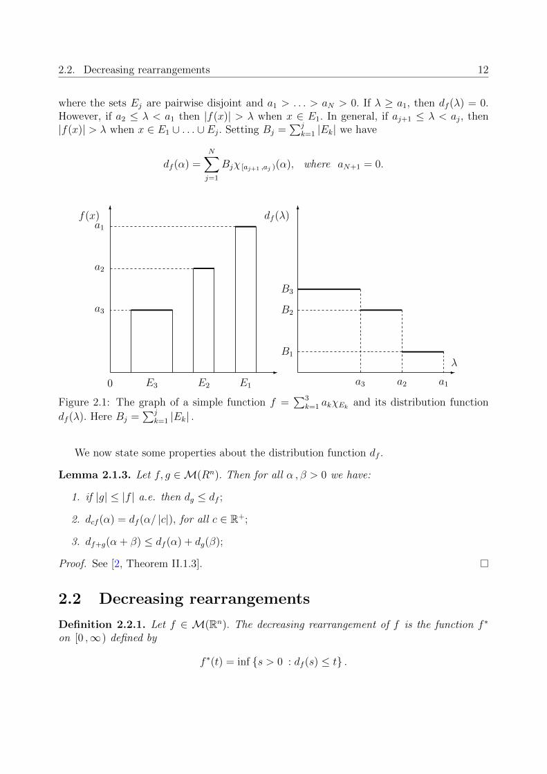
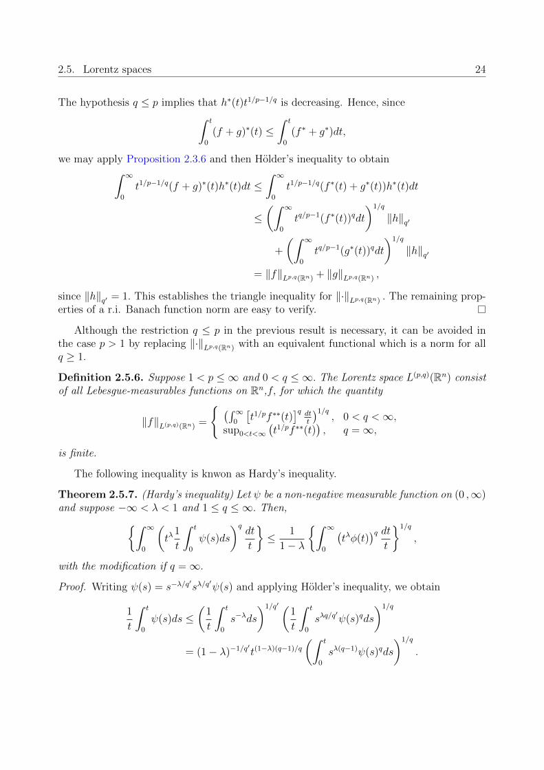
Example 2.1.2. Recall that simple functions are finite linear combinations of characteristicfuctions of sets of finite measure. Now, we compute the distribution function df of a non-negative simple function
f(x) =N∑j=1
ajχEj(x), (2.1)
11
2.2. Decreasing rearrangements 12
where the sets Ej are pairwise disjoint and a1 > . . . > aN > 0. If λ ≥ a1, then df (λ) = 0.However, if a2 ≤ λ < a1 then |f(x)| > λ when x ∈ E1. In general, if aj+1 ≤ λ < aj, then|f(x)| > λ when x ∈ E1 ∪ . . . ∪ Ej. Setting Bj =
∑jk=1 |Ek| we have
df (α) =N∑j=1
Bjχ [aj+1 ,aj )(α), where aN+1 = 0.
6
-
6
-
E3 E2 E1
a1
0
f(x)
B3
B2
B1
df (λ)
a3 a2 a1
a3
a2
λ
Figure 2.1: The graph of a simple function f =∑3
k=1 akχEk and its distribution function
df (λ). Here Bj =∑j
k=1 |Ek| .
We now state some properties about the distribution function df .
Lemma 2.1.3. Let f, g ∈M(Rn). Then for all α , β > 0 we have:
1. if |g| ≤ |f | a.e. then dg ≤ df ;
2. dcf (α) = df (α/ |c|), for all c ∈ R+;
3. df+g(α + β) ≤ df (α) + dg(β);
Proof. See [2, Theorem II.1.3].
2.2 Decreasing rearrangements
Definition 2.2.1. Let f ∈ M(Rn). The decreasing rearrangement of f is the function f ∗
on [0 ,∞) defined by
f ∗(t) = inf s > 0 : df (s) ≤ t .
13 Chapter 2. Preliminaries
We adopt the convention inf ∅ = ∞, thus having f ∗(t) = ∞ whenever df (α) > t for allα ≥ 0. Note that f ∗ is decreasing.
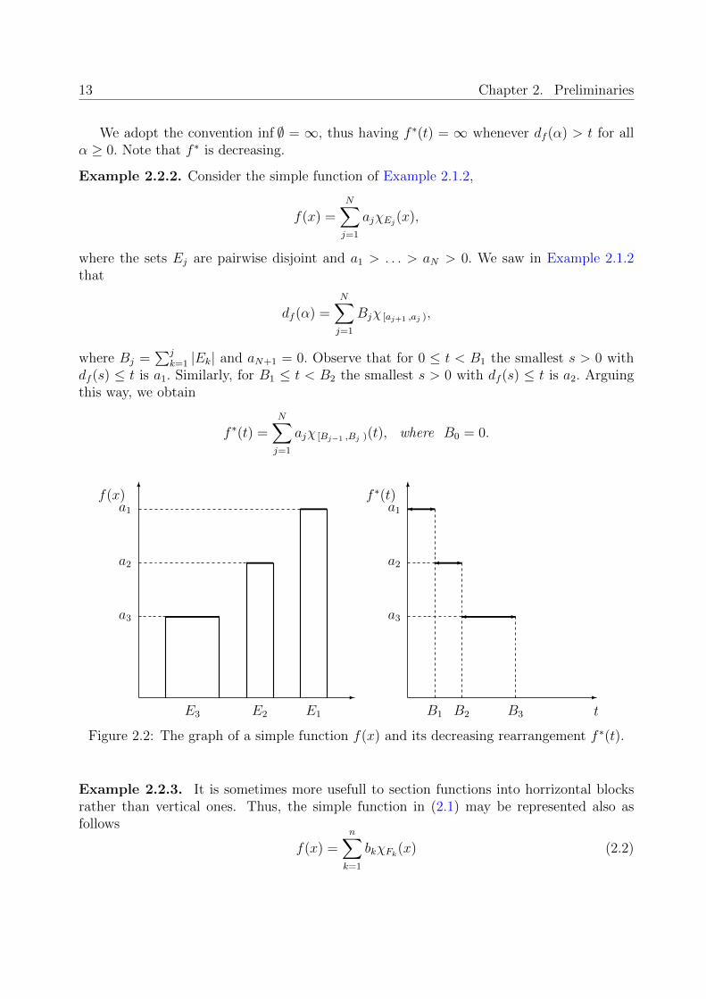
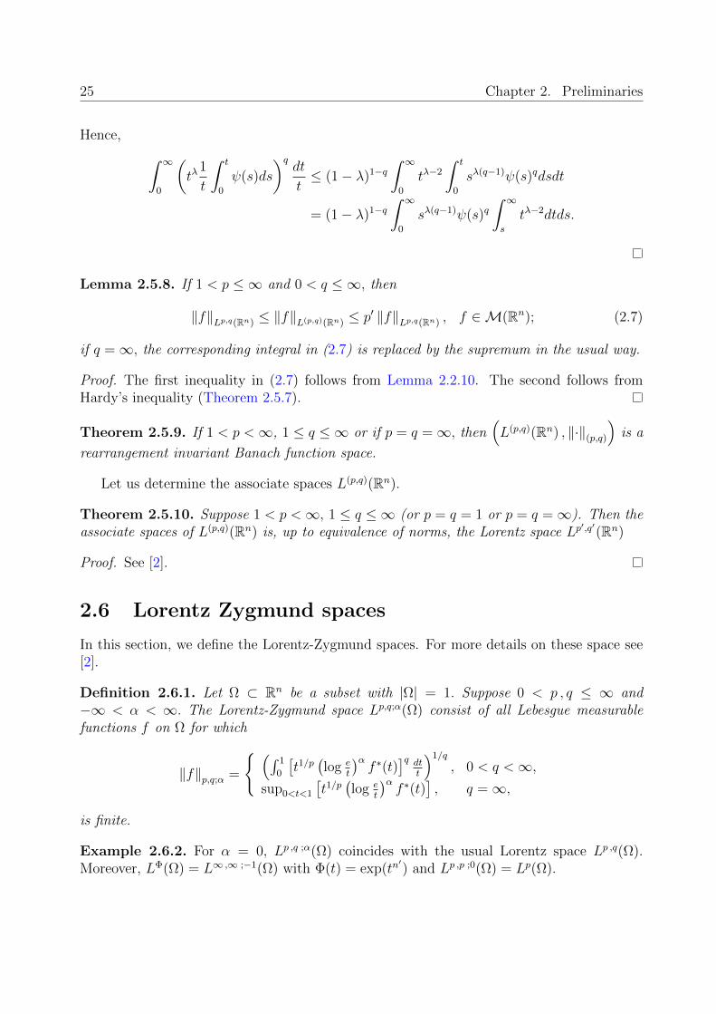
Example 2.2.2. Consider the simple function of Example 2.1.2,
f(x) =N∑j=1
ajχEj(x),
where the sets Ej are pairwise disjoint and a1 > . . . > aN > 0. We saw in Example 2.1.2that
df (α) =N∑j=1
Bjχ [aj+1 ,aj ),
where Bj =∑j
k=1 |Ek| and aN+1 = 0. Observe that for 0 ≤ t < B1 the smallest s > 0 withdf (s) ≤ t is a1. Similarly, for B1 ≤ t < B2 the smallest s > 0 with df (s) ≤ t is a2. Arguingthis way, we obtain
f ∗(t) =N∑j=1
ajχ [Bj−1 ,Bj )(t), where B0 = 0.
6
-
6
-
a1
a2
f(x)
E3 E2 E1
-
-
-
a1
a2
a3
f ∗(t)
B1 B2 B3 t
a3
Figure 2.2: The graph of a simple function f(x) and its decreasing rearrangement f ∗(t).
Example 2.2.3. It is sometimes more usefull to section functions into horrizontal blocksrather than vertical ones. Thus, the simple function in (2.1) may be represented also asfollows
f(x) =n∑k=1
bkχFk(x) (2.2)
2.2. Decreasing rearrangements 14
where the coefficients bk are positive and the sets Fk each have finite measure and form anincreasing sequenece F1 ⊂ F2 ⊂ . . . ⊂ Fn. Comparison with (2.1) shows that
bk = ak − ak+1, Fk = ∪kj=1Ej, k = 1 , 2 , . . . , n.
Thus
f ∗(t) =n∑k=1
bkχ[ 0 ,|Fk|) (t).
Lemma 2.2.4. Suppose f and g belong to M(Rn) and let α be any scalar.
1. f ∗ is a right-continuous function on [0 ,∞) ;
2. if |g| ≤ |f | a.e. then g∗ ≤ f ∗;
3. (αf)∗ = |α| f ∗;
4. (f + g)∗(t1 + t2) ≤ f ∗(t1) + g∗(t2); (t1 , t2 ≥ 0);
5. df (f∗(t)) ≤ t for all 0 ≤ t <∞;
6. f and f ∗ have the same distribution function.
The following lemma is useful in proving other properties of f ∗, since it allows us toreduce these proofs to the case when f is a simple funcion.
Lemma 2.2.5. Let fm ∈ M(Rn), such that for all x ∈ Rn, |fm(x)| ≤ |fm+1(x)|, m ≥ 1.If f is a measurable function satisfying
|f(x)| = limm→∞
|fm(x)| , x ∈ Rn,
then for each t > 0, f ∗m(t) ↑ f ∗(t).
Proof. It follows from Lemma 2.2.4 that f ∗m(t) ≤ f ∗m+1(t) ≤ f ∗(t) for m ≥ 1. Let
` = limm→∞
f ∗m(t).
Since f ∗m(t) ≤ `, we have
dfm(`) ≤ dfm (f ∗(t)) ≤ t, thus df (`) = limm→∞
dfm(`) ≤ t.
Hence, f ∗(t) ≤ `. But, from the inequality f ∗m(t) ≤ f ∗(t) we obtain ` ≤ f ∗(t). It thereforefollows that ` = f ∗(t) and the lemma is proved.
Proposition 2.2.6. Let f ∈M(Ω). If 0 < p <∞, then∫Rn|f(x)|p dx =
∫ ∞0
f ∗(t)pdt.
Moreover, if p =∞, ‖f‖∞ = f ∗(0).
15 Chapter 2. Preliminaries
Proof. In view of Lemma 2.2.5, we will prove this property for an arbitary non-negativesimple function f. Using Example 2.2.2 we have∫
Rn|f(x)|p dx =
N∑j=1
apj |Ej| =∫ ∞
0
N∑j=1
apjχ [Bj−1 ,Bj )(t)dt =
∫ ∞0
(f ∗(t))p dt.
We continue with some properties of f ∗.
Theorem 2.2.7. If f and g belong to M+(Rn), then∫Rn|f(x)| |g(x)| dx ≤
∫ ∞0
f ∗(s)g∗(s)ds. (2.3)
To prove this theorem we require the following lemma. Its proof can be found in [2].
Lemma 2.2.8. Let g be a non-negative simple function and let E be an arbitrary measurablesubset of Rn. Then ∫
E
g(x)dx ≤∫ |E|
0
g∗(s)ds.
Proof. (Theorem 2.2.7) It is enough to establish (2.3) for non-negative functions f and g.There is no loss of generality in assuming f and g to be simple. In that case, we may write
f(x) =m∑j=1
ajχEj(x),
where E1 ⊂ E2 ⊂ . . . ⊂ Em and aj > 0 , j = 1 , 2 , . . . ,m. Then
f ∗(t) =m∑j=1
ajχ [0 ,|Ej |) (t).
Hence, by Lemma 2.2.8,∫Rnf(x)g(x)dx =
m∑j=1
aj
∫Ej
g(x)dx ≤m∑j=1
aj
∫ |Ej |0
g∗(s)ds
=
∫ ∞0
m∑j=1
ajχ [0 ,|Ej | )(s)g∗(s)ds =
∫ ∞0
f ∗(s)g∗(s)ds
Definition 2.2.9. Let f be a Lebesgue-measurable function on Rn. Then f ∗∗ will denote themaximal function of f ∗ defined by
f ∗∗(t) =1
t
∫ t
0
f ∗(s)ds (t > 0) .
2.3. Rearrangement invariant Banach function spaces 16
Some properties of the maximal function, f ∗∗, are listed in the following lemma, whichis proved in [2].
Lemma 2.2.10. Suppose f, g and fn belong to M(Rn) and let α be any scalar. Then f ∗∗
is non-negative, decreasing and continuous on (0 ,∞) . Furthermore, the following propertieshold:
• f ∗∗ ≡ 0 if and only if f ≡ 0 a.e;
• f ∗ ≤ f ∗∗;
• if |g| ≤ |f | a.e. then g∗∗ ≤ f ∗∗;
• (αf)∗∗ = |α| f ∗∗;
• (f + g)∗∗(t) ≤ f ∗∗(t) + g∗∗(t)
• if |fn| ↑ |f | a.e. then f ∗∗n ↑ f ∗∗.
2.3 Rearrangement invariant Banach function spaces
Definition 2.3.1. A rearrangement-invariant (r.i.) Banach function norm ρ on M+(Rn)satisfies the following axioms
• ρ(f) ≥ 0 with ρ(f) = 0 if and only if f = 0 a.e. on Rn;
• ρ(cf) = cρ(f), c ∈ R+;
• ρ(f + g) ≤ ρ(f) + ρ(g);
• fn ↑ f implies ρ(fn) ↑ ρ(f);
• E ⊂ Rn with |E| <∞, then ρ(χE) <∞;
• E ⊂ Rn with |E| <∞, then∫Ef(x)dx / ρ(f);
• f ∗ = g∗, then ρ(f) = ρ(g)
Definition 2.3.2. Let ρ be a r.i. Banach functin norm. The collection, X(Rn), of allfunction f in M(Rn) for which ρ (|f |) < ∞ is called a rearrangement-invariant Banachfunction space. For each f ∈ X(Ω), define
‖f‖X(Rn) = ρ (|f |) .
17 Chapter 2. Preliminaries
Definition 2.3.3. Given a r.i. space X(Rn), the set
X ′ =
f ∈M(Rn) ;
∫Ω
|f(x)g(x)| dx <∞ for every g ∈ X(Rn)
,
endowed with the norm
‖f‖X′(Rn) = sup‖g‖X(Rn)≤1
∫Rn|f(x)g(x)| ,
is called the associate space of X(Rn).
Proposition 2.3.4. Let X(Rn) be an r.i. Banach function space. Then the associate X ′(Ω)is also an r.i. Banach function space. Furthermore,
‖f‖X′(Rn) = sup‖g‖X(Rn)≤1
∫Rnf ∗(t)g∗(t)dt, and ‖f‖X(Rn) = sup
‖g‖X′(Rn)≤1
∫Rnf ∗(t)g∗(t)dt.
A basic tool for working with r.i. spaces is the Hardy-Littlewood-Polya principle:
Theorem 2.3.5. Let X(Rn) be an r.i. Banach function spaces. If f ∗∗(t) ≤ g∗∗(t) for allt > 0, then ‖f‖X(Rn) ≤ ‖g‖X(Rn) .
To prove this theorem we will use the following result. For this result see [2].
Proposition 2.3.6. Let f1 and f2 be non-negative measurable functions on (0 ,∞) andsuppose ∫ t
0
f1(s)ds ≤∫ t
0
f2(s)ds,
for all t > 0. Let h be any non-negative decreasing function on (0 ,∞) . Then,∫ ∞0
f1(s)h∗(s)ds ≤∫ ∞
0
f2(s)h∗(s)ds.
Proof. (Theorem 2.3.5) By Proposition 2.3.4, it needs only be shown that∫ ∞0
f ∗(s)h∗(s)ds ≤∫ ∞
0
g∗1(s)h∗(s)ds,
for every g such that ‖g‖X′(Rn) ≤ 1. But this is an immediate consequence of Proposi-
tion 2.3.6, since∫ t
0f ∗(t)dt ≤
∫ t0g∗(t)dt and h∗ is non-negative and decreasing.
Theorem 2.3.7. (Luxemburg representation theorem). Let Ω ⊂ Rn be an open subset. Letρ be a rearrangement-invariant function norm on M+(Ω). Then, there is a (not necessarilyunique) rearrangement-invariant function norm ρ on M+(I), where I = (0 , |Ω|) , such that
ρ(f) = ρ(f ∗), ∀f ∈M+(Ω).
2.4. Orlicz spaces 18
Furthemore, if σ is any rearrangement-invariant function norm on M+(I) which representρ, in the sense that
ρ(f) = σ(f ∗), f ∈M+(Ω),
then the associate norm ρ′ of ρ is representaed in the same way by the associate norm σ′ ofσ, that is
ρ′(g) = σ′(g), g ∈M+(I).
2.4 Orlicz spaces
Now, we recall the definition of Orlicz spaces. For a detailed treatment of Orlicz spaces, werefer to [2].
Definition 2.4.1. Let φ : [0 ,∞)→ [0 ,∞] be increasing and left-continuous function withφ(0) = 0. Suppose on (0 ,∞) that φ is neither identically zero nor identically infinite. Thenthe function Φ defined by
Φ(s) =
∫ s
0
φ(u)du, (s ≥ 0)
is said to be a Young’s function.
Remark 2.4.2. Note that a Young’s function is convex on the interval where it is finite.Indeed, given s , t ≥ 0 and λ ∈ (0 , 1) we have
Φ (λs+ (1− λ)t) =
∫ λs+(1−λ)t
0
φ(r)dr =
∫ s
0
φ(r)dr +
∫ λs+(1−λ)t
s
φ(r)dr
= λ
∫ s
0
φ(r)dr + (1− λ)
∫ s
0
φ(r)dr +
∫ λs+(1−λ)t
s
φ(r)dr. (2.4)
Since φ is increasing and left continuous we have∫ λs+(1−λ)t
s
φ(r)dr ≤ (1− λ)(t− s)φ (λs+ (1− λ)t)
∫ t
λs+(1−λ)t
φ(r)dr ≥ λ(t− s)φ (λs+ (1− λ)t) .
Then, comparing the two previous inequalities we obtain
λ
∫ λs+(1−λ)t
s
φ(r)dr ≤ (1− λ)
∫ t
λs+(1−λ)t
φ(r)dr,
19 Chapter 2. Preliminaries
and so, ∫ λs+(1−λ)t
s
φ(r)dr = λ
∫ λs+(1−λ)t
s
φ(r)dr + (1− λ)
∫ λs+(1−λ)t
s
φ(r)dr
≤ (1− λ)
∫ λs+(1−λ)t
s
φ(r)dr + (1− λ)
∫ t
λs+(1−λ)t
φ(r)dr
= (1− λ)
∫ t
s
φ(r)dr. (2.5)
Finally, plugging (2.5) in (2.4), we obtain
Φ (λs+ (1− λ)t) ≤ λ
∫ s
0
φ(r)dr + (1− λ)
∫ t
0
φ(r)dr = λΦ(s) + (1− λ)Φ(t).
Moreover, note that lims→∞Φ(s)/s =∞. Indeed, for all t > 0 we have
Φ(t)
t=
1
t
∫ t
0
φ(s)ds ≥ 1
t
∫ t
t/2
φ(s)ds ≥ 1
2φ
(t
2
),
and then, letting t→∞, we obtain the desired result.
Definition 2.4.3. Let Φ be a Young’s function. The Luxemburg norm ρΦ is defined by
ρΦ(f) = infk > 0 : MΦ(kf) ≤ 1
, f ∈M(Rn), (2.6)
where
MΦ(kf) =
∫Rn
Φ
(|f(x)|k
)dx.
Remark 2.4.4. If ρΦ(f) > 0, the infimun in (2.6) is attained. Indeed, we denote
A =
k > 0 :
∫Rn
Φ
(|f(x)|k
)dx ≤ 1
.
Let kn ∈ A be a decreasing sequence. We claim that limn kn = ρΦ(f). In fact, given ε > 0,there exists kn such that kn − ρΦ(f) < ε, since ρΦ(f) is the infimum of A. Then, if n < Nwe have
kN − ρΦ(f) < kn − ρΦ(f) < ε,
and so limn kn = ρΦ(f). Thus Φ (|f(x)| /kn) ↑ Φ(|f(x)| /ρφ(f)
), beucase Φ is left-continuous.
Finally, we obtain, by monotone convergence,∫Rn
Φ
(|f(x)|ρφ(f)
)dx ≤ 1.
Therefore ρΦ(f) ∈ A and
ρΦ(f) = min
k > 0 :
∫Rn
Φ
(|f(x)|k
)dx ≤ 1
.
2.4. Orlicz spaces 20
In order to show that ρΦ is an r.i. norm, we shall need the following preliminary result.
Lemma 2.4.5. If Φ is a Young’s function, then
f = 0 a.e. ⇔ MΦ(kf) ≤ 1, ∀ k > 0.
Proof. Suppose f = 0 a.e. Then ρΦ(f) = 0 and so MΦ(kf) ≤ 1 for all k > 0. Conversely,suppose that MΦ(kf) ≤ 1 for all k > 0, but for some ε > 0 we have |f | ≥ ε on a set E ofpositive measure. Then
MΦ(kf) ≥∫E
Φ(kε)dx = |E|Φ(kε).
Since Φ(s) ↑ ∞ as s ↑ ∞, we therefore obtain the contradiction that MΦ(kf) ↑ ∞ ask ↑ ∞.
Theorem 2.4.6. If Φ is a Young’s function, then ρΦ is an r.i. norm.
Proof. We need to verify the following properties:
• ρΦ(f) = 0 ⇔ f = 0 a.e. Indeed, it follows from Lemma 2.4.5.
• ρΦ(αf) = αρφ(f) ∀α > 0. It is suffices to consider ρΦ(f) > 0. We have∫Ω
Φ
(α |f(x)|αρΦ(f)
)dx =
∫Ω
Φ
(|f(x)|ρΦ(f)
)dx ≤ 1,
hence ρΦ (αf) ≤ αρΦ(f). On the other hand, since∫
ΩΦ(α|f(x)|ρΦ(αf)
)dx ≤ 1, we have
ρΦ(f) ≤ ρΦ (αf) /α.
• ρφ (f + g) ≤ ρΦ(f) + ρΦ(g), for all f , g ∈M(Rn). Indeed, let γ = ρΦ(f) + ρΦ(g) <∞and let α = ρΦ(f)/γ and β = ρΦ(g)/γ with α + β = 1. By (2.6),
MΦ(f/ρΦ(f)
)≤ 1 and MΦ
(g/ρΦ(g)
)≤ 1.
Since Φ is convex, we have
MΦ
(f + g
γ
)= MΦ
(αf
ρΦ(f)+
βg
ρΦ(g)
)≤ αMΦ
(f
ρΦ(f)
)+ βMΦ
(g
ρΦ(g)
)≤ α + β = 1.
Hence, we conclude that ρΦ (f + g) ≤ γ = ρΦ(f) + ρΦ(g).
• 0 ≤ g ≤ f a.e. ⇒ ρΦ(g) ≤ ρΦ(f). Indeed, 0 < ρΦ(f) <∞. Then
MΦ
(g
ρΦ(f)
)≤MΦ
(f
ρΦ(f)
),
and ρΦ(g) < ρΦ(f).
21 Chapter 2. Preliminaries
• 0 ≤ fn ↑ f a.e. ⇒ ρΦ(fn) ↑ ρΦ(f). Indeed, by the above property, the sequence ρΦ(fn)is increasing. Let αn = ρΦ(fn) and put α = supαn. Since ρΦ(f) ≥ αn for each n, itfollows that ρΦ(f) ≥ α. We must show ρΦ(f) ≤ α. This is clear for α = 0 or α = ∞,so we may assume that 0 < αn <∞ for all n ≥ 1. In this case
MΦ
(fnα
)≤MΦ
(fnαn
)≤ 1,
and the monotone convergence theorem shows that the quantity on the left convergesto MΦ
(fα
). Hence MΦ
(fα
)≤ 1, and therefore ρΦ(f) ≤ α.
• Let E ⊂ Rn any measurable subset. Let b denote the measure of E (we may assumeb > 0). We claim that,
ρΦ(χE) <∞.
Indeed, the Young’s function Φ is not identically infinite on (0 ,∞) , and it is continuouson the interval where it is finite. Since Φ(0) = 0, it follows that there is a number k > 0for which Φ(k) ≤ 1/b. Then MΦ(kχE) = bΦ(k) ≤ 1 and hence ρΦ(χE) ≤ 1/k <∞.
• Let E be a subset of Rn of measure b > 0. Let f ∈M(Rn) with 0 < ρΦ(f) <∞. Withk = 1/ρΦ(|f |), Jensen’s inequality gives
Φ
(1
b
∫E
k |f(x)| dx)≤ 1
b
∫E
Φ (k |f(x)|) dx ≤ 1
bMΦ(kf) ≤ 1
b.
Hence, since Φ increases to ∞, there is a constant c ,which depends on Φ and b, suchthat
1
b
∫E
k |f(x)| dx ≤ c ⇒∫E
|f(x)| dx ≤ cbρΦ(f).
• The rearrangement-invariance follows from the fact that MΦ(f) = MΦ(g) whenever fand g are equimesurables. The latter property needs only be established with g = f ∗.There is no loss of generality in assuming f to be a simple function. In that case,we may write f(x) =
∑Nj=1 ajχEj(x), where the sets Ej are pairwise disjoint and
a1 > . . . > aN . Then,
f ∗(t) =N∑j=1
ajχ [Bj−1 ,Bj )(t), where Bj =N∑j=1
|Ej| and B0 = 0.
So,
MΦ(f) =
∫Rn
Φ
(N∑j=1
ajχEj(x)
)dx =
N∑j=1
|Ej|Φ(aj),
2.5. Lorentz spaces 22
and
MΦ(f ∗) =
∫ ∞0
Φ
(N∑j=1
ajχ [Bj−1 ,Bj )(t)
)dx =
N∑j=1
∫ Bj
Bj−1
Φ(aj)dx
=N∑j=1
(Bj −Bj−1)Φ(aj) =N∑j=1
|Ej|Φ(aj).
Hence, MΦ(f) = MΦ(f ∗).
Definition 2.4.7. Let Φ be a Young’s function. The Orlicz space is the rearrangementinvariant Banach function space of those f ∈M(Rn) for which the Luxemburg norm
‖f‖LΦ = ρΦ(f),
is finite.
Example 2.4.8. If we take φ(u) = pup−1, where 1 ≤ p <∞, then Φ(u) = up and the Orliczspace LΦ(Rn) is the Lp(Rn).
2.5 Lorentz spaces
This section contains definition and some results from Lorentz spaces that will appear lateron. For more information on Lorentz spaces see [2] and [13].
Definition 2.5.1. Given f ∈M(Rn) and 0 < p, q ≤ ∞, define
‖f‖Lp,q(Rn) =
(∫∞0
[t1/pf ∗(t)
]q dtt
)1/q, 0 < q <∞,
sup0<t<∞(t1/pf ∗(t)
), q =∞.
The set of all f ∈M(Rn) with ‖f‖Lp,q(Rn) <∞ is denoted by Lp,q(Rn) and is called Lorentzspace.
Remark 2.5.2. Using the notation of Example 2.2.2, when 0 < q <∞ we have
‖f‖Lp,q(Rn) =
(p
q
)1/q [aq1B
q/p1 + aq2
(Bq/p2 −Bq/p
1
)+ . . .+ aqN
(Bq/pN −B
q/pN−1
)]1/q
.
It follows that the only simple function with finite ‖·‖L∞,q(Rn) norm is identically equal tozero; for this reason we have that L∞,q(Rn) = 0 , for any 0 < q <∞
The next result shows that, for any fixed p, the Lorentz spaces increase as the secondexponent q increases.
23 Chapter 2. Preliminaries
Proposition 2.5.3. Suppose 0 < p <∞ and 1 ≤ q ≤ r ≤ ∞. Then
Lp,q(Rn) → Lp,r(Rn).
Proof. Suppose r =∞. Using the fact that f ∗ is decreasing, we have
t1/pf ∗(t) =
(p
q
∫ t
0
[s1/pf ∗(t)
]q dss
)1/q
≤(p
q
∫ t
0
[s1/pf ∗(s)
]q dss
)1/q
≤(p
q
)1/q
‖f‖Lp,q(Rn) .
Hence, taking the supremum over all t > 0, we obtain
‖f‖Lp,∞(Rn) ≤(p
q
)1/q
‖f‖Lp,q(Rn) .
Now, suppose r <∞, we have
‖f‖Lp,r(Rn) =
(∫ ∞0
[t1/pf ∗(t)
]r−q+q dtt
)1/r
≤ ‖f‖1−q/rLp,∞(Rn) ‖f‖
q/rLp,q(Rn)
≤(p
q
)(r−q)/rq
‖f‖Lp,q(Rn) .
Note that ‖·‖Lp,q(Rn) , does not satisfy the triangle inequality if p < q ≤ ∞..
Example 2.5.4. Consider f(t) = t and g(t) = 1−t defined on [0 , 1] . Then f ∗(λ) = g∗(λ) =1 − λ. A calculation shows that the triangle inequality for these functions with respect tothe norm ‖·‖Lp ,q(Rn) would be equivalent to
p
q≤ 2
Γ(q + 1)Γ(p/q)
Γ(q + 1 + q/p).
So, if we take q = 2 and p = 4, we will obtain 2 ≤ 1/12.
However, there is the following result.
Theorem 2.5.5. Suppose 1 ≤ q ≤ p <∞ or p = q =∞. Then,(Lp,q(Rn) , ‖·‖Lp,q(Rn)
)is a
rearrangement-invariant Banach function space.
Proof. The result is clear when p = q = 1 or p = q = ∞ since Lp ,q(Rn) reduces to theLebesgue spaces L1(Rn) and L∞(Rn), respectively. Hence, we may assume that 1 < p <∞and 1 ≤ q ≤ p. We have
‖f + g‖Lp,q(Rn)=sup‖h‖Lq′=1
∫ ∞0
(f + g)∗(t)h∗(t)dt,
2.5. Lorentz spaces 24
The hypothesis q ≤ p implies that h∗(t)t1/p−1/q is decreasing. Hence, since∫ t
0
(f + g)∗(t) ≤∫ t
0
(f ∗ + g∗)dt,
we may apply Proposition 2.3.6 and then Holder’s inequality to obtain∫ ∞0
t1/p−1/q(f + g)∗(t)h∗(t)dt ≤∫ ∞
0
t1/p−1/q(f ∗(t) + g∗(t))h∗(t)dt
≤(∫ ∞
0
tq/p−1(f ∗(t))qdt
)1/q
‖h‖q′
+
(∫ ∞0
tq/p−1(g∗(t))qdt
)1/q
‖h‖q′
= ‖f‖Lp,q(Rn) + ‖g‖Lp,q(Rn) ,
since ‖h‖q′ = 1. This establishes the triangle inequality for ‖·‖Lp,q(Rn) . The remaining prop-erties of a r.i. Banach function norm are easy to verify.
Although the restriction q ≤ p in the previous result is necessary, it can be avoided inthe case p > 1 by replacing ‖·‖Lp,q(Rn) with an equivalent functional which is a norm for allq ≥ 1.
Definition 2.5.6. Suppose 1 < p ≤ ∞ and 0 < q ≤ ∞. The Lorentz space L(p,q)(Rn) consistof all Lebesgue-measurables functions on Rn,f, for which the quantity
‖f‖L(p,q)(Rn) =
(∫∞0
[t1/pf ∗∗(t)
]q dtt
)1/q, 0 < q <∞,
sup0<t<∞(t1/pf ∗∗(t)
), q =∞,
is finite.
The following inequality is knwon as Hardy’s inequality.
Theorem 2.5.7. (Hardy’s inequality) Let ψ be a non-negative measurable function on (0 ,∞)and suppose −∞ < λ < 1 and 1 ≤ q ≤ ∞. Then,∫ ∞
0
(tλ
1
t
∫ t
0
ψ(s)ds
)qdt
t
≤ 1
1− λ
∫ ∞0
(tλφ(t)
)q dtt
1/q
,
with the modification if q =∞.
Proof. Writing ψ(s) = s−λ/q′sλ/q
′ψ(s) and applying Holder’s inequality, we obtain
1
t
∫ t
0
ψ(s)ds ≤(
1
t
∫ t
0
s−λds
)1/q′ (1
t
∫ t
0
sλq/q′ψ(s)qds
)1/q
= (1− λ)−1/q′t(1−λ)(q−1)/q
(∫ t
0
sλ(q−1)ψ(s)qds
)1/q
.
25 Chapter 2. Preliminaries
Hence, ∫ ∞0
(tλ
1
t
∫ t
0
ψ(s)ds
)qdt
t≤ (1− λ)1−q
∫ ∞0
tλ−2
∫ t
0
sλ(q−1)ψ(s)qdsdt
= (1− λ)1−q∫ ∞
0
sλ(q−1)ψ(s)q∫ ∞s
tλ−2dtds.
Lemma 2.5.8. If 1 < p ≤ ∞ and 0 < q ≤ ∞, then
‖f‖Lp,q(Rn) ≤ ‖f‖L(p,q)(Rn) ≤ p′ ‖f‖Lp,q(Rn) , f ∈M(Rn); (2.7)
if q =∞, the corresponding integral in (2.7) is replaced by the supremum in the usual way.
Proof. The first inequality in (2.7) follows from Lemma 2.2.10. The second follows fromHardy’s inequality (Theorem 2.5.7).
Theorem 2.5.9. If 1 < p <∞, 1 ≤ q ≤ ∞ or if p = q =∞, then(L(p,q)(Rn) , ‖·‖(p,q)
)is a
rearrangement invariant Banach function space.
Let us determine the associate spaces L(p,q)(Rn).
Theorem 2.5.10. Suppose 1 < p <∞, 1 ≤ q ≤ ∞ (or p = q = 1 or p = q =∞). Then theassociate spaces of L(p,q)(Rn) is, up to equivalence of norms, the Lorentz space Lp
′,q′(Rn)
Proof. See [2].
2.6 Lorentz Zygmund spaces
In this section, we define the Lorentz-Zygmund spaces. For more details on these space see[2].
Definition 2.6.1. Let Ω ⊂ Rn be a subset with |Ω| = 1. Suppose 0 < p , q ≤ ∞ and−∞ < α < ∞. The Lorentz-Zygmund space Lp,q;α(Ω) consist of all Lebesgue measurablefunctions f on Ω for which
‖f‖p,q;α =
(∫ 1
0
[t1/p
(log e
t
)αf ∗(t)
]q dtt
)1/q
, 0 < q <∞,sup0<t<1
[t1/p
(log e
t
)αf ∗(t)
], q =∞,
is finite.
Example 2.6.2. For α = 0, Lp ,q ;α(Ω) coincides with the usual Lorentz space Lp ,q(Ω).Moreover, LΦ(Ω) = L∞ ,∞ ;−1(Ω) with Φ(t) = exp(tn
′) and Lp ,p ;0(Ω) = Lp(Ω).
2.7. Interpolation spaces 26
2.7 Interpolation spaces
This section contains definitions and results from interpolation theory that will appear lateron. For a detailed treatment of interpolation spaces, we refer to [2].
Definition 2.7.1. A pair (X0 , X1) of Banach spaces X0 and X1 is called a compatible coupleif there is some Hausdorff topological vector space in which each of X0 and X1 is continuouslyembedded.
Any pair (X , Y ) of Banach spaces for which X is continuously embedded in Y (or viceversa) is a compatible couple, beucase we may choose for the Hausdorff space the space Yitself.
Theorem 2.7.2. Let (X0 , X1) be a compatible couple. Then X0 + X1 and X0 ∩ X1 areBanach spaces under the norms
‖f‖X0+X1= inf
f=f0+f1
‖f0‖X0
+ ‖f1‖X1
, and ‖f‖X0∩X1
= max‖f‖X0
, ‖f‖X1
,
respectively.
Proof. See [2, Theorem V.1.3].
Definition 2.7.3. Let (X0 , X1) be a compatible couple of Banach spaces. The PeetreK-functional is defined for each f ∈ X0 +X1 and t > 0 by
K (f, t;X0, X1) = inf‖f0‖X0
+ t ‖f1‖X1: f = f0 + f1
,
where the infimum extends over all representations f = f0 + f1 of f with f0 ∈ X0 andf1 ∈ X1.
Example 2.7.4. Consider the compatiple couple (L1(Ω) , L∞(Ω)) . Then
K(f, t;L1(Ω), L∞(Ω)) =
∫ t
0
f ∗(s)ds.
Theorem 2.7.5. Let T be an admisible linear operator with respect to compatible couples(X0 , X1) and (Y0 , Y1) . Then
K(Tf, t;Y0, Y1) ≤M0K(f, tM1/M0;X0, X1)
for all f in X0 +X1 and all t > 0.
Proof. The admisible operator T satisfies
‖Tfi‖Yi ≤Mi ‖fi‖Xi , fi ∈ Xi , i = 0, 1.
27 Chapter 2. Preliminaries
If f ∈ X0 + X1 and f = f0 + f1 is any decomposition of f with fi ∈ Xi (i = 0 , 1), thenTf = Tf0 + Tf1 and Tfi ∈ Yi, (i = 0 , 1). Hence,
K(Tf, t;Y0, Y1) ≤ ‖Tf0‖X0+ t ‖Tf1‖Y1
≤M0
(‖f0‖X0
+ tM0
M1
‖f1‖X1
).
Taking the infimum over all such representations f = f0 + f1 of f , we obtain
K(Tf, t;Y0, Y1) ≤M0K(f, tM1/M0;X0, X1).
Definition 2.7.6. Let (X0 , X1) be a compatible couple. The space (X0 , X1)θ,q consist of allf in X0 +X1 for which the functional
‖f‖θ,q =
(∫∞0
[t−θK(f, t)
]q dtt
)1/q, 0 < θ < 1 , 1 ≤ q <∞,
supt>0 t−θK(f, t), 0 ≤ θ ≤ 1 , q =∞,
is finite where K(f, t) = K(f, t,X0, X1).
Theorem 2.7.7. Let (X0 , X1) be a compatible couple of Banach spaces. Then (X0 , X1)θ,qendowed with the norm ‖·‖θ,q is a Banach space.
X0 ∩X1 → (X0 , X1)θ,q → X0 +X1.
Example 2.7.8. An important example is the case X0 = L1(Ω), X1 = L∞(Ω) for which thecorresponding interpolation spaces are the Lorentz spaces: for 1 < p < ∞ and 1 ≤ q ≤ ∞one write
Lp,q(Ω) =(L1(Ω) , L∞(Ω)
)1/p′,q
.
Remark 2.7.9. Let (X0 , X1) be a compatible couple and consider two interpolation spaces
Xθ0 = (X0 , X1)θ0 ,q0 , Xθ1 = (X0 , X1)θ1 ,q1 ,
where 0 < θ0 < θ1 < 1 and 1 ≤ q0 , q1 < ∞. Then(Xθ0 , Xθ1
)is itself a compatible
couple. The following theorem relates the K-functional of the underlying couples (X0 , X1)and
(Xθ0 , Xθ1
). Its proof may be found in [16]. We shall write
K(f , t) = K(f, t;X0, X1), and K(f, t) = K(f, t;Xθ0 , Xθ1).
Theorem 2.7.10. Let (X0 , X1) be a compatible couple and consider two interpolation spaces
Xθ0 = (X0 , X1)θ0 ,q0 , Xθ1 = (X0 , X1)θ1 ,q1 ,
where 0 < θ0 < θ1 < 1 and 1 ≤ q0 , q1 ≤ ∞. Then
K(f, t) ≈
(∫ 1/ν
0
(s−θ0K(f, t)
)q0 dss
)1/q0
+ t
(∫ ∞1/ν
(s−θ1K(f, t)
)q1 dss
)1/q1
,
where ν = θ1 − θ0.
2.8. Weighted Hardy operators 28
Remark 2.7.11. With the same technique we can estimate K(f, t) in the two extremecases K(f, t;X0, Xθ1) and K(f, t;Xθ1 , X1). The result in these two cases is
K(f, t;X0, Xθ1) ≈ t
(∫ ∞t1/θ1
(s−θ1K(f, s)
)q1 dss
)1/q1
K(f, t;Xθ0 , X1) ≈
(∫ t1/(1−θ0)
0
(s−θ0K(f, s)
)q0 dss
)1/q0
.
2.8 Weighted Hardy operators
Let n ≤ 2 and 1 ≤ m ≤ n − 1. We establish properties of Weighted Hardy operadors.Throughout this section we present results proved in [18].
Lemma 2.8.1. Let Hn/m and H ′n/m be the associate weighted Hardy operators defined by
(Hn/mf)(t) :=
∫ 1
t
f(s)sm/n−1ds (H ′n/mf)(t) := tm/n−1
∫ t
0
f(s)ds,
f ∈M+(I) , t ∈ I = (0 , 1) . Then,
Hn/m : L1(I)→ Ln/(n−m),1(I), Hn/m : Ln/m,1(I)→ L∞(I), (2.8)
and
H ′n/m : L1(I)→ Ln/(n−m),∞(I), H ′n/m : Ln/m,∞(I)→ L∞(I). (2.9)
Remark 2.8.2. Note that Hn/mf is nonincreasing in t. Indeed, let t1 < t2 ∈ I. Then,
Hn/m(t2) =
∫ 1
t2
f(s)sm/n−1ds <
∫ 1
t1
f(s)sm/n−1ds = Hn/m(t1).
Proof. (Lemma 2.8.1). Let us prove (2.8).
∥∥Hn/mf∥∥Ln/(n−m),1(I)
=
∫ 1
0
(Hn/mf(t)
)∗∗t−m/ndt =
∫ 1
0
t−m/n−1
(∫ t
0
(Hn/mf
)(y)dy
)/∫ 1
0
s−m/n(∫ 1
s
f(t)tm/n−1dt
)ds ≈
∫ 1
0
f(t)dt = C ‖f‖L1(I) .
Hence, Hn/m : L1(I)→ Ln/(n−m),1(I). Now,
∥∥Hn/mf∥∥L∞(I)
= sup0<t<1
(Hn/mf
)∗(t) ≤
∫ 1
0
f(s)sm/n−1ds ≤∫ 1
0
f ∗(s)sm/n−1ds = ‖f‖Ln/m,1(I).
29 Chapter 2. Preliminaries
Therefore, Hn/m : Ln/m,1(I)→ L∞(I). Let us prove (2.9).
∥∥H ′n/mf∥∥Ln/(n−m),∞(I)= sup
g 6=0
∫ 1
0(H
′
n/mf)(t)g(t)dt
‖g‖Ln/m,1(I)
= supg 6=0
∫ 1
0(Hn/mg)(t)f(t)dt
‖g‖Ln/m,1(I)
≤ supg 6=0
∥∥Hn/mg∥∥L∞(I)
‖f‖L1(I)
‖g‖Ln/m,1(I)
/ ‖f‖L1(I) .
Therefore, H ′n/m : L1(I)→ Ln/(n−m),∞(I). Finally,
∥∥H ′n/m∥∥L∞(I)= sup
g 6=0
∫ 1
0(H ′n/mf)(t)g(t)dt
‖g‖L1(I)
= supg 6=0
∫ 1
0(Hn/mg)(t)f(t)dt
‖g‖L1(I)
≤ supg 6=0
∥∥Hn/mg∥∥Ln/(n−m),1(I)
‖f‖Ln/m,∞(I)
‖g‖L1(I)
/ ‖f‖Ln/m,∞(I) .
Hence, the proof is complete.
Additional results involving Hn/m and H ′n/m require the supremum operator Tn/m definedby
(Tn/mf)(t) := t−m/n supt≤s<1
sm/nf ∗(s), with f ∈M(I) and t ∈ I.
Remark 2.8.3. Note that (Tn/mf)(t) is non-increasing in t. Indeed, let t1 ≤ t2 < 1. Wehave
t−m/n2 sup
t2≤s<1sm/nf ∗(s) ≤ t
−m/n1 sup
t2≤s<1sm/nf ∗(s) ≤ t
−m/n1 sup
t1≤s<1sm/nf ∗(s),
that is (Tn/mf)(t2) ≤ (Tn/mf)(t1).
Lemma 2.8.4. The operators Tn/m have the following endpoint mapping properties:
Tn/m : Ln/m,∞(I)→ Ln/m,∞(I), (2.10)
andTn/m : L1(I)→ L1(I). (2.11)
Proof. Let us prove (2.10)
∥∥Tn/mf∥∥Ln/m,∞(I)= sup
0<t<1tm/n−1
∫ t
0
s−m/n sups≤y<1
ym/nf ∗(y)ds
≤ sup0<t<1
tm/n−1
∫ t
0
s−m/n sup0≤y<1
ym/nf ∗∗(y)ds
≈ ‖f‖Ln/m,∞(I) .
2.8. Weighted Hardy operators 30
Now, let us prove (2.11). It sufficies to verify∥∥Tn/mf∥∥L1 ≤ ‖f‖L1 , for f ∈ D(I). Given such
an f 6= 0, define
(Rf)(t) = supt≤s<1
sm/nf ∗(s),
and set A = k ∈ N : (Rf)(rk) > (Rf)(rk−1) , where rk is given by∫ rk
0
t−m/ndt =n
n−m2−k;
that is, rk = 2−nk/(n−m), k = 0, 1, . . . Then, A is non-empty. Take k ∈ A and define
zk =
0 if (Rf)(t) = (Rf)(rk), t ∈ (0 , rk ];min rj ; (Rf)(rj) = (Rf)(rk) otherwise.
Note that,
Rf(0) = sup0≤s<1
sm/nf ∗(s) = sup0<s≤1
sm/nf ∗(s) = sup0<u<1
supu<s≤1
sm/nf ∗(s)
= sup0<u<1
Rf(u) = sup0<u<rk
Rf(u) = Rf(rk).
Thus,
(Rf)(t) = (Rf)(rk), k ∈ A , t ∈ [zk , rk] .
Moreover, by the definition of A, suprk≤t<1 tm/nf ∗(t) is attained in [rk , rk−1 ) when k ∈ A.
Therefore, for every k ∈ A and t ∈ [zk , rk−1 ) , we have
(Rf)(t) ≤ (Rf)(rk) = suprk≤s<rk−1
sm/nf ∗(s) ≤ rm/nk−1 f
∗(rk).
So, ∥∥Tn/mf∥∥L1(I)≤∑k∈A
∫ rk−1
zk
(Rf)(t)t−m/ndt+
∫ 1
rk0
(Rf)(t)t−m/ndt
≤∑k∈A
rm/nk−1 f
∗(rk)
∫ rk−1
0
t−m/ndt ≤∑k∈A
rk−1f∗(rk)
/∑k∈A
∫ rk
rk+1
f ∗(t)dt ≤ ‖f‖L1(I) ,
where k0 = max k ∈ A .
We continue with some further properties of Tn/m
Theorem 2.8.5. Let X(I) be an r.i. space. Then,∥∥tm/n(Tn/mf∗∗)(t)
∥∥X(I)
/∥∥tn/mf ∗∗(t)∥∥
X(I).
31 Chapter 2. Preliminaries
The following two lemmas are essential to the proof of Theorem 2.8.5.
Lemma 2.8.6. For all f ∈M(I) and t ∈ I(Tn/mf
)∗∗(t) ≤
(Tn/mf
∗∗) (t).
Proof. Given f ∈M+(I) and t ∈ I, set
ft(s) = min [f(s), f ∗(t)] , f t(s) = max [f(s)− f ∗(t) , 0] , s ∈ (0 , 1) .
Then,
(ft)∗(s) = min [f ∗(s), f ∗(t)] , (f t)∗(s) = (f ∗(s)− f ∗(t))χ(0,t)(s),
and so, f ∗(s) = (ft)∗(s) + (f t)∗(s), s ∈ I. Since, (Tn/mf)(t) is noncreasing in t,(
Tn/mf)∗∗
(t) =1
t
∫ t
0
s−m/n sups≤y<1
ym/nf ∗(y)ds
≤ 1
t
∫ t
0
s−m/n sups≤y<1
ym/n(ft)∗(y)ds+
1
t
∫ t
0
s−m/n sups≤y<1
ym/n(f t)∗(y)ds
= I + II.
Since,
I =1
t
∫ t
0
s−m/n sups≤y<1
ym/n min [f ∗(y), f ∗(t)] ds
=1
t
∫ t
0
s−m/n max
[sups≤y<t
ym/nf ∗(t) , supt≤y<1
ym/nf ∗(y)
]ds
=1
t
∫ t
0
s−m/n supt≤y<1
ym/nf ∗(y)ds
=n
n−mt−m/n sup
t≤y<1ym/nf ∗(y) =
n
n−m(Tn/mf
)(t),
and
II =1
t
∫ t
0
s−m/n sups≤y<1
ym/n(f t)∗(y)ds ≤ 1
t
∫ 1
0
(Tn/mf
t)
(s)ds
≤ 1
t
∫ 1
0
(f t)∗(s)ds
=1
t
∫ t
0
[f ∗(s)− f ∗(t)] ds ≤ f ∗∗(t).
We conclude that, for f ∈M+(I), t ∈ I,(Tn/mf
)∗∗(t) / f ∗∗(t) + (Tn/mf)(t) /
(Tn/mf
∗∗) (t).
2.8. Weighted Hardy operators 32
Lemma 2.8.7. Let X(I) be an r.i. spaces. Then,∥∥∥∥ supt≤s<1
sm/nf ∗∗(s)
∥∥∥∥X(I)
/∥∥tm/nf ∗∗(t)∥∥
X(I), t ∈ I.
Proof. We only need to prove∫ t
0
sup0≤y<1
ym/nf ∗∗(y)ds ≤ C
∫ t
0
(ym/nf ∗∗(y)
)∗ (s2
)ds.
with C > 0 independent of f ∈ M+(I), since in that case by the Hardy-Littlewood-Polyaprinciple we will obtain the result:∥∥∥∥ sup
t≤s<1sm/nf ∗∗(s)
∥∥∥∥X(I)
/∥∥E1/2(ym/nf ∗∗(y))
∥∥X(I)
/∥∥sm/nf ∗∗(s)∥∥
X(I).
To this end, fix f ∈M+(I) and t ∈(0 , 1
3
)and take ft and f t as in the proof of Lemma 2.8.6.
Then
sups≤y<1
ym/nf ∗∗(y) = sups≤y<1
ym/n[(ft)
∗∗(y) + (f t)∗∗(y)]
≤ sups≤y<1
ym/n(ft)∗∗(y) + sup
s≤y<1ym/n(f t)∗∗(y).
Now,
(f t)∗∗(y) =
f ∗∗(y)− f ∗(t), 0 < y < t,ty
[f ∗∗(t)− f ∗(t)] , t ≤ y < 1.
Hence, for 0 < s ≤ t
sups≤y<1
ym/n(f t)∗∗(y) ≤ max
[sups≤y<t
ym/nf ∗∗(y) , supt≤y<1
ym/n−1tf ∗∗(t)
]≤ sup
s≤y≤tym/nf ∗∗(y),
and so ∫ t
0
sups≤y<1
ym/n(f t)∗∗(y)ds ≤∫ t
0
sups≤y≤t
ym/n−1
∫ y
0
f ∗(z)dzds
≤(∫ t
0
sups≤y≤t
ym/n−1ds
)(∫ t
0
f ∗(s)ds
)≤ n
mtm/n
∫ t
0
f ∗(s)ds.
But, since∫ 2t
tg ≤
∫ t0g∗ and g
( ·2
)∗(s) = g∗
(s2
),∫ t
0
(ym/nf ∗∗(y)
)∗ (s2
)ds ≥
∫ 2t
t
(s2
)m/nf ∗∗(s
2
)ds ≥ 2−m/ntm/n+1f ∗∗(t)
= 2−m/ntm/n∫ t
0
f ∗(s)ds,
33 Chapter 2. Preliminaries
which yields ∫ t
0
sups≤y<1
ym/n(f t)∗∗
(y)ds ≤ n
m2m/n
∫ t
0
(ym/nf ∗∗(y)
)∗ (s2
)ds.
To prove ∫ t
0
sups≤y<1
ym/n (ft)∗∗ (y)ds ≤ C
∫ t
0
(ym/nf ∗∗(y)
)∗ (s2
)ds
we will show there is a constant C > 0 so that, for each f ∈M+(I),
sups≤y<1
ym/n (ft)∗∗ (y) ≤ C sup
t≤y<1ym/n−1
∫ y
t
f ∗(z
2
)dz, 0 < s < 1 , 0 < t <
1
3, (2.12)
and, moreover
sm/nf ∗∗(s
2
)= sm/n−1
∫ s
0
f ∗(z
2
)dz ≥ C−1 sup
t≤y<1ym/n−1
∫ y
t
f ∗(z
2
)dz, (2.13)
on a set of measure al least t. This will suffice, since the right-hand side of (2.12) does notdepend on s. Let us prove (2.12):
(ft)∗∗(y) = f ∗(t)χ(0,t)(y) +
[t
yf ∗(t) +
1
y
∫ y
t
f ∗(z)dz
]χ [t ,1 )(y),
whence
sups≤y<1
ym/n(ft)∗∗(y) ≤ tm/nf ∗(t) + sup
t≤y<1ym/n−1
∫ y
t
f ∗(z)dz
≤ (2−m/n+1 + 1) supt≤y<1
ym/n−1ym/n−1
∫ y
t
f ∗(z
2
)dz,
since
supt≤y<1
ym/n−1
∫ y
t
f ∗(z
2
)≥ (2t)m/n−1
∫ 2t
t
f ∗(z
2
)dz ≥ 2m/n−1tm/nf ∗(t).
Thus, (2.12) holds with C = (2−m/n+1 +1). Now, let’s prove (2.13). Next, suppose y0 ∈ (t , 1]is such that
supt≤y<1
ym/n−1
∫ y
t
f ∗(z
2
)dz = y
m/n−10
∫ y0
t
f ∗(z
2
)dz.
We consider two cases.
2.8. Weighted Hardy operators 34
• Let y0 ≤ 2t. First note that t < y0 implies (2y0)m/n−1 ≤ (y0 + t)m/n−1 . Next, sincey0/2 ≤ t and f ∗ is decreasing,∫ y0
0
f ∗(z
2
)dz ≥ 2
∫ y0
t
f ∗(z
2
)dz.
Altogether, for y0 < s < y0 + t, we have
sm/n−1
∫ s
0
f ∗(z
2
)dz ≥ (y0 + t)m/n−1
∫ y0
0
f ∗(z
2
)dz ≥ 2m/ny
m/n−10
∫ y0
t
f ∗(z
2
)dz
= 2m/n supt≤y<1
ym/n−1
∫ y
t
f ∗(z
2
)dz.
• Let y0 ≥ 2t. For y0 − t < s < y0, we have
sm/n−1
∫ s
0
f ∗(z
2
)dz ≥ y
m/n−10
∫ y0−t
0
f ∗(z
2
)dz ≥ y
m/n−10
∫ y0
t
f ∗(z
2
)dz
= supt≤y<1
ym/n−1
∫ y
t
f ∗(z
2
)dz.
Therefore, the proof is complete.
Proof. (Theorem 2.8.5). By Lemma 2.8.6 we have (Tn/mf)∗∗(t) ≤ (Tn/mf∗∗)(t). Then by
Lemma 2.8.7 we have∥∥tm/n(Tn/mf)∗∗(t)∥∥X(I)≤∥∥tm/n(Tn/mf
∗∗)(t)∥∥X(I)
=
∥∥∥∥ supt≤s<1
sm/nf ∗∗(s)
∥∥∥∥X(I)
/∥∥sm/nf ∗∗(s)∥∥
X(I).
Chapter 3
Sobolev spaces
3.1 Introduction
In this chapter, we present a brief description of those aspects of distributions that arerelevant for our purposes. Of special importance is the notion of weak or distributionalderivative of an integrable function. We also define the Sobolev spaces and collect their mostimportant properties. We conclude this chapter proving the Sobolev embedding theorem.Such theorem tells us that W 1Lp(Rn) → Lq(Rn) for certain values of q depending on p andn.
3.2 Definitions and basic properties
Consider an open set Ω ⊂ Rn and fix a compact set K ⊂ Ω. We define
Dk(Ω) = f ∈ C∞(Ω) : supp f ⊂ K .
We say that φk → φ in Dk(Ω) if Dαφk → Dαφ uniformly for every α ∈ Nn.
Definition 3.2.1. Let Ω ⊂ Rn be an open subset. A distribution on Ω is a linear mappingu : D(Ω)→ C such that for every compact set, K ⊂ Ω, u|Dk(Ω) ∈ Dk(Ω)′. We denote D′(Ω)the complex linear space of all distributions on Ω.
Remark 3.2.2. Let f ∈ L1loc(Ω) and 〈φ , f〉 =
∫Ωf(x)φ(x)dx. Then uf = 〈. , f〉 belongs to
D′(Ω). Indeed, let K ⊂ Ω be a compact subset and let φk ∈ Dk(Ω) such that φk → 0 inDk(Ω) (i.e Dαφk → 0 uniformly for every α ∈ Nn) ; we have
|〈φk , f〉| =∣∣∣∣∫K
φk(x)f(x)dx
∣∣∣∣ ≤ ‖φk‖∞ ∫K
f(x)dx.
Then uf (φk) → 0; hence uf ∈ D′(Ω). The linear mapping f ∈ L1loc → 〈. , f〉 ∈ D(Ω) is one
to one, so we may consider L1loc(Ω) ⊂ D′(Ω) and therefore Lp(Ω) ⊂ D′(Ω) for 1 ≤ p ≤ ∞,
since Lp(Ω) ⊂ L1loc(Ω) for 1 ≤ p ≤ ∞.
35
3.2. Definitions and basic properties 36
Definition 3.2.3. Let α = (α1 , . . . αn) ∈ Nn and f ∈ L1loc(Ω), we define the distributional
derivatives of f , Dα, as follows∫Ω
Dαf(x)φ(x)dx = (−1)|α|∫
Ω
f(x)Dαφ(x)dx ∀φ ∈ D(Ω),
where |α| = α1 + . . .+ αn.
Definition 3.2.4. Let Ω ⊂ Rn be an open set, 1 ≤ p ≤ ∞ and m ∈ N. The Sobolev space oforder m ∈ N is defined by
WmLp(Ω) := u ∈ Lp(Ω) ;Dαu ∈ Lp(Ω) , |α| ≤ m ,
where Dαu represent the distributional derivatives of u.
Theorem 3.2.5. Let Ω ⊂ Rn an open set, 1 ≤ p ≤ ∞ and m ∈ N. The space WmLp(Ω) isa Banach space with the norm
‖u‖WmLp(Ω) =
∑0≤|α|≤m ‖Dαu‖Lp(Ω) , if 1 ≤ p <∞,
max0≤|α|≤m ‖Dαu‖L∞(Ω) , if p =∞.
Proof. Let un be a Cauchy sequence in WmLp(Ω). Then Dαun is a Cauchy sequence inLp(Ω) for 0 ≤ |α| ≤ m. Since Lp(Ω) is complete, there exit u , uα ∈ Lp(Ω), such that un → uand Dαun → uα in Lp(Ω) norm as n→∞. We claim that un → u in D′(Ω). Indeed, for anyφ ∈ D(Ω) we have ∫
Ω
|un(x)− u(x)| |φ(x)| dx ≤ ‖φ‖p′ ‖un − u‖p → 0
as n→∞. Similary Dαun → ua in D′(Ω). It follows that
limn→∞
∫Ω
Dαun(x)φ(x)dx = limn→∞
(−1)α∫
Ω
un(x)Dαφ(x)dx = (−1)α∫
Ω
u(x)Dαφ(x)dx
=
∫Ω
Dαu(x)φ(x)dx.
Thus uα = Dαu in the distributional sense on Ω for 0 ≤ |α| ≤ m, whence u belongs toWmLp(Ω). Moreover, we have limn→∞ ‖un − u‖WmLp(Ω) = 0, and so the space WmLp(Ω) iscomplete.
Proposition 3.2.6. Let 1 ≤ p <∞. Then D(Rn) is dense in WmLp(Rn).
Proof. Let be φ ∈ D(Rn) such that∫Rn φ(x)dx = 1. For every ε > 0, we consider φε(x) :=
ε−nφ(x/ε). Let f ∈ WmLp(Rn), and set fε := f ∗ φε. We have fε ∈ C∞(Rn); moreover
37 Chapter 3. Sobolev spaces
f ∗ φε → f in Lp-norm as ε→ 0. Indeed,∫Rn|f ∗ φε(x)− f(x)|p dx ≤
∫Rn
(∫Rn|f(x− y)− f(x)|φε(y)dy
)pdx
≤∫Rn
(∫Rn|f(x− y)− f(x)|p φε(y)dy
)dx
×(∫
Rnφε(y)dy
)1/p′
=
∫Rn‖τyf − f‖Lp(Rn) φε(y)dy
=
∫Rn‖τεyf − f‖Lp(Rn) φ(y)dy
then by the Lebesque dominated convergence and the fact that ‖τεyf − f‖p → 0 as ε → 0,we obtain the desire result. Moreover, Dαfε → Dαf in Lp-norm, as ε → 0, ∀α ∈ Nn suchthat 1 ≤ |a| ≤ m. Note that ∀ψ ∈ D(Rn)∫
RnDαfε(x)ψ(x)dx = (−1)|α|
∫Rn
(∫Rnf(x− y)φε(y)dy
)Dαψ(x)dx
= (−1)|α|∫Rn
(∫Rnf(x− y)Dαψ(x)dx
)φε(y)dy
=
∫Rn
(∫RnDαxf(x− y)ψ(x)dx
)φε(y)dy
=
∫RnDαf ∗ φε(x)ψ(x)dx.
Thus, we have Dαfε → Dαf, since Dαf ∈ Lp. Note that the functions fε give the re-quired aproximation, but they not have compact support. So we need to introduce thetwo-paremetrer family
τδ(η)fε ∈ D(Rn) , δ , ε ∈ R+,
with η ∈ D(Rn) such that η(0) = 1. Fix ε > 0, if we prove,
Dα(τδ(η)fε)→ Dα(fε)
in Lp-norm as δ → 0 for all 0 ≤ |α| ≤ m, where τδ(η)(x) is the dilation operador defined by
τδ(η)(x) := η(δx), δ ∈ R+;
we will complete the proof. Indeed, if |α| = 0 since
limδ→0
η(δx)fε(x) = fε(x) and |η(δx)fε(x)| ≤ |fε(x)| a.e.,
using the Lebesgue dominated convergence we obtain the desire result. Next, if 1 ≤ |a| ≤ m,
limδ→0
Dα(η(δx)fε(x)) = Dαfε(x) and |Dα(η(δx)fε(x))| ≤ |fε(x)|+ |Dαfε(x)| a.e.
3.3. Riesz potencials 38
Then, by the Lebesgue dominated convergence, we obtain the desire result. Therefore, theproof is complete.
The following example shows that the proposition is not true for an arbitrary domainΩ ⊂ Rn.
Example 3.2.7. Let Ω = (x , y) ∈ R2 : 0 < |x| < 1 , 0 < y < 1 . Let u be a function de-fined on Ω.
u(x , y) =
1 if x > 00 if x < 0.
Denote K = Ω. Suppose that there exists φ ∈ C1(K) such that ‖u− φ‖W 1 ,p(Ω) < ε. Let
L = (x , y) : −1 ≤ x ≤ 0 , 0 ≤ y ≤ 1 , R = (x , y) : 0 ≤ x ≤ 1 , 0 ≤ y ≤ 1 .
We have ‖φ‖L1(L) ≤ ‖φ‖Lp(L) < ε and similarly ‖1− φ‖L1(R) < ε, from which we obtain
‖φ‖L1(R) > 1 − ε. Let Φ(x) =∫ 1
0φ(x , y)dy, by the Integral Mean Value Theorem, we know
that there exists a and b with −1 < a < 0 and 0 < b < 1 such that Φ(a) < ε and Φ(b) > 1−ε.If 0 < ε < 1/2
1− 2ε < Φ(b)− Φ(a) =
∫ b
a
Φ′(x)dx ≤
∫Ω
|Dxφ(x , y)| dxdy ≤ 21/p′ ‖Dxφ‖Lp(Ω) .
Hence, 1 < ε(2 + 21/p′), which is impossible for small ε. The problem with this domain isthat lie on both sides of part of its boundary. The condition which is called the segmentcondition prevents this from happening and guarantees that D(Rn) is dense in WmLp(Ω)for 1 ≤ p <∞.
3.3 Riesz potencials
Definition 3.3.1. Let 0 < α < n and f ∈ D(Rn). We define the Riesz potencials by
Iα(f)(x) =1
γ(α)
∫Rn|x− y|−n+α f(y)dy, with γ(α) =
πn/22αΓ(α/2)
Γ(n/2− α/2). (3.1)
with γ(α) = πn/22αΓ(α/2)Γ(n/2−α/2)
.
Remark 3.3.2. Since the Riesz potencials are integral operators it is natural to inquire abouttheir actions on the spaces Lp(Rn). We formulate the following problem: given α , 0 < α < nfor what pairs p and q, is the operator f → Iα(f) bounded from Lp(Rn) to Lq(Rn). Supposethat we had an estimate
‖Iα(f)‖Lq(Rn) ≤ C ‖f‖Lq(Rn) ,
39 Chapter 3. Sobolev spaces
for some positive indices p , q and all f ∈ Lp(Rn). Then p and q must be related by
1
q=
1
p− α
n.
In fact, let f ∈ D(Rn) non-negative. Consider the dilation operador defined by
τδ(f)(x) = f(δx), δ ∈ R+.
Then
Iα(τδf)(x) =1
γ(α)
∫Rn|x− y|−n+α f(δy)dy =
1
γ(α)
∫Rn|x− z/δ|−n+α f(z)δ−ndy
=1
γ(α)
∫Rn|δx− z|−n+α f(z)δ−αdy = δατδ(Iαf)(x);
thus
‖Iα(τδ(f))‖q = δ−α ‖τδIαf‖q = δ−α−n/q ‖Iαf‖q ≤ C ‖τδf‖p = Cδ−n/p ‖f‖p .
Hence
‖Iαf‖q ≤ Cδ−1/p+1/q+α/n ‖f‖p .
Suppose now that 1/p > 1/q + α/n, letting δ → ∞ obtain that Iα(f) = 0.Similary, if1/p < 1/q + α/n letting δ → 0, we obtain that ‖f‖p = ∞. Thus, this inequality is possibleonly if 1/q = 1/p− α/n.
Theorem 3.3.3. Let 0 < α < n , 1 ≤ p < q <∞, 1/q = 1/p− α/n. If f ∈ L1(Rn), then
|x : |Iαf(x) > λ|| ≤(A ‖f‖1
λ
)q.
Proof. Let be K(x) = |x|−n+α , we consider the transformation f → K ∗ f (which differsfrom f → Iαf by a contant multiple). We decompose K as K1 +K∞ where
K1(x) =
K(x), if |x| ≤ µ0 if |x| > µ
K∞(x) =
K(x), if |x| > µ0 if |x| ≤ µ
with µ a fixed positive constant which need not to be specified. Note that K1 ∈ L1(Rn) andK∞ ∈ Lp
′. Suppose that ‖f‖pp = 1. Since K ∗ f = K1 ∗ f +K∞ ∗ f, we have
|x : |K ∗ f(x)| > 2λ| ≤ |x : |K1 ∗ f(x)| > λ|+ |x : |K∞ ∗ f | (x) > λ|
3.4. Sobolev embedding theorem 40
However
|x : |K1 ∗ f(x)| > λ| ≤‖K1 ∗ f‖pp
λp≤‖K1‖p1 ‖f‖
pp
λp=‖K1‖p1λp
= cµα
λp,
since
‖K1‖1 =
∫|x|≤µ|x|−n+α dx = cµα.
Next‖K∞ ∗ f‖∞ ≤ ‖K∞‖p′ ‖f‖p = ‖K∞‖p′ = cµ−n/q,
since
‖K∞‖p′ =
(∫|x|>µ|x|(−n+α)p′ dx
)1/p′
= cµ−n/q.
Now, if cµ−n/q = λ, we obtain ‖K∞‖p′ = λ. Take µ = cλ−q/m to have this value; then‖K∞ ∗ f‖∞ ≤ λ and so |x : |K∞ ∗ f(x)| > λ| = 0. Finally
|x : |K ∗ f(x)| > 2λ| ≤ cµα
λ
p
= cλ−q = c
(‖f‖pλ
)qHence, the mapping f → K ∗ f is of weak type (p , q), in particular when p = 1.
Theorem 3.3.4. Let 0 < α < n and 1 < p < q <∞ with 1/q = 1/p− α/n. Then,
‖Iαf‖q ≤ Ap ,q ‖f‖p .
Proof. It follows from Theorem 3.3.3 and the Marcinkiewicz interpolation theorem.
3.4 Sobolev embedding theorem
In this section, we will study the Sobolev embedding theorem. It asserts that:
• if 1 ≤ p < n, then W 1Lp(Rn) → Lq(Rn) where p∗ = np/(n− p);
• if p = n, then W 1Lp(Rn) → Lq(Rn), for every p ≤ q <∞;
• if p > n, then W 1Lp(Rn) → L∞(Rn).
Embeddings: 1 ≤ p < n
Theorem 3.4.1. Let n ≥ 2. If 1 < p < n, then
W 1Lp(Rn) → Lp∗(Rn), where p∗ =
pn
n− p.
To prove this theorem, we need the following lemma. It gives an appropriate way ofexpressing a function in terms of its partial derivates. Its proof can be found in [27].
41 Chapter 3. Sobolev spaces
Lemma 3.4.2. Let f ∈ D(Rn) then
f(x) =1
ωn−1
n∑j=1
∫Rn
Dj(x− y)yj|y|n
dy,
where ωn−1 is the area of the sphere Sn−1.
Proof. (Theorem 3.4.1) Assume that f ∈ D(Rn). By Lemma 3.4.2 we have
|f(x)| /n∑j=1
∫Rn|Djf(x− y)| |y|−n+1 dy =
n∑j=1
I1 (Djf) (x).
Hence, we get
‖f‖qLq(Rn) /∫Rn
∣∣∣∣∣n∑j=1
I1 (Djf) (x)
∣∣∣∣∣q
dx /n∑j=1
∫Rn|I1 (Djf) (x)|q dx /
n∑j=1
‖Djf‖pLp(Rn) .
Now, let f ∈ W 1Lp(Rn). Since D(Rn) is dense in W 1 ,p(Rn), there exists fk ∈ D(Rn) suchthat ‖fk − f‖W 1 ,p(Rn) → 0. Hence, we get
‖fk − fk′‖Lq(Rn) /n∑j=1
‖Djfk −Djfk′‖Lp(Rn) ,
and so the sequence fk also converges in Lq(Rn) norm and this limit is equal f. Thusf ∈ Lq(Rn) and
‖f‖Lq(Rn) /n∑j=1
‖Djf‖Lp(Rn) / ‖f‖W 1Lp(Rn) .
This shows that f ∈ Lq(Rn) and the inclusion mapping of W 1Lp(Rn) into Lq(Rn) is contin-uous.
At the end of fifties, Gagliardo [12] and Nirenberg [22] extended Theorem 3.4.1 to thecase p = 1. Note that the argument used in Theorem 3.4.1 does not work in case p = 1beucase Theorem 3.3.4 fails for p = 1. A different idea is neeeded and it is contained in thenext lemma, which is proved in [19]. We use the notation xk for the vector in Rn−1 obtainedfrom a given x ∈ Rn by removing its kth coordenate, that is
xk = (x1 , . . . , , xk−1 , xk+1 , . . . , xn) ∈ Rn−1.
Lemma 3.4.3. Let n ≥ 2. Assume that the functions gk ∈ L1(Rn−1) k = 1 , . . . , n arenon-negative. Then∫
Rn
n∏k=1
gk(xk)1/(n−1)dx ≤
(n∏k=1
∫Rn−1
gk(xk)dxk
)1/(n−1)
.
3.4. Sobolev embedding theorem 42
Proof. The proof is by induction on n. If n = 2, let
g(x) := g1(x2)g2(x1) with x = (x1 , x2) ∈ R2.
Using Tonelli’s theorem we get∫R2
g(x)dx =
(∫Rg1(x2)dx2
)(∫Rg2(x1)dx1
).
Assume next that the result is true for n and let us prove it for n+ 1. Let
g(x) =n+1∏k=1
gi(xi)1/n, with gi ∈ L1(Rn).
Fix xn+1 ∈ R. Integrating both sides of the previous identity with respect to x1 , . . . , xn andusing Holder’s inequality, we get
∫Rng(x)dxn+1 ≤
(∫Rngn+1(xn+1)dxn+1
)1/n(∫
Rn
n∏k=1
gk(yk , xn+1)1/(n−1)dy
)1−1/n
where y = (x1 , . . . , xn). Since xn+1 is fixed, by induction hypothesis we have(∫Rn
n∏k=1
gk(yk , xn+1)1/(n−1)dy
)1−1/n
≤
(n∏k=1
∫Rn−1
gk(yk , xn+1)dyk
)1/n
.
Thus ∫Rng(x)dxn+1 ≤
(∫Rngn+1(xn+1)dxn+1
)1/n(
n∏k=1
∫Rn−1
gk(yk , xn+1)dyk
)1/n
.
Integrating both sides of the previous identity with respect xn+1 and using Holder’s inequalitywe get ∫
Rng(x)dx ≤
(n+1∏k=1
∫Rngk(xk)dxk
)1/n
.
Theorem 3.4.4. Let n ≥ 2 and p = 1. Then,
W 1L1(Rn) → Ln′(Rn).
Proof. Let f ∈ D(Rn), we have
|f(x)| ≤ 1
2
∫R|Dkf(x)| dxk ≡ gk(xk) k = 1 , . . . , n.
43 Chapter 3. Sobolev spaces
Applying Lemma 3.4.3 we obtain∫Rn|f(x)|n/(n−1) dx ≤
∫Rn
n∏k=1
gk(xk)1/(n−1)dx ≤
(n∏k=1
∫Rn−1
gk(xk)dxk
)1/(n−1)
≤ 1
2n/(n−1)
n∏k=1
‖Dkf‖1/(n−1)
L1(Rn) ;
hence
‖f‖Ln′ (Rn) ≤1
2
(n∏k=1
‖Dkf‖L1(Rn)
)1/n
.
If we use the fact that(∏n
j=1 aj
)1/n
≤ 1n
∑nj=1 aj if aj ≥ 0; then as consequence we have
‖f‖Ln′ (Rn) ≤1
2n
n∑k=1
‖Dkf‖L1(Rn) . (3.2)
Now, let f ∈ W 1L1(Rn). Since D(Rn) is dense in W 1 ,1(Rn), there exists fm ∈ D(Rn) suchthat ‖f − fm‖W 1L1(Rn) → 0, as m→∞. Hence, by (3.2) we have
‖fm − fm′‖Ln′ ≤1
2n
n∑k=1
‖Dkfm −Dkfm′‖L1(Rn) ,
hence f ∈ Ln′(Rn), and
‖f‖Ln′ (Rn) ≤1
2n
n∑k=1
‖Dkf‖L1(Rn) ≤1
2n‖f‖W 1L1(Rn) .
Corollary 3.4.5. Let n ≥ 2. Let k be a positive integer such that 1 ≤ k ≤ n − 1. Suppose1 ≤ p < n/k. Then,
W 1Lp(Rn) → Lp∗(Rn), with p∗ =
np
n− kp.
Proof. The proof proceeds by induction on k. Note that Theorem 3.4.1 and Theorem 3.4.4establish the case k = 1. Now, assume that
‖v‖Lqk−1 (Rn) / ‖v‖Wk−1Lp(Rn) , v ∈ Wk−1Lp(Rn),
where qk−1 = npn−kp+p . Let u ∈ W kLp(Rn); we take v = Dju 1 ≤ j ≤ n we obtain
‖Dju‖Lqk−1 (Rn) / ‖Dju‖Wk−1Lp(Rn) .
3.4. Sobolev embedding theorem 44
Therefore,
‖u‖W 1Lqk−1 (Rn) =n∑j=1
‖Dju‖Lqk−1 (Rn) /n∑j=1
∑0≤|α|≤k−1
‖DαDju‖Lp(Rn) / ‖u‖WkLp(Rn) .
Now, since kp < n, we have qk−1 < n and so
‖u‖Lq(Rn) / ‖u‖W 1Lqk−1 (Rn) / ‖u‖WkLq(Rn) ,
where q = nqk−1
n−qk−1= np
n−kp .
Embeddings: p = n
We have seen that for a given function u ∈ W 1Lp(Rn) and 1 ≤ p < n, then
‖u‖Lp∗ (Rn) / ‖u‖W 1Lp(Rn) ,
where p∗ = np/(n − p). Note that when p tends to n, p∗ tends to ∞ and so one would betempted to say that if u ∈ W 1Ln(Rn) then u ∈ L∞(Rn). The following example shows thatthis is false if n > 1.
Example 3.4.6. Put n = 2 and define u(x) := log log(
1 + 1|x|
). Let us prove that u ∈
W 1L2 (B(0 , 1)) . Indeed, it suffices to prove that for all k = 0 , . . . , n there is a positiveconstant, c > 0, such that∣∣∣∣∫
B(0 ,1)
u(x)Dkφ(x)dx
∣∣∣∣ ≤ c ‖Dkφ‖2 ∀φ ∈ D (B(0 , 1)) . (3.3)
Indeed, if (3.3) holds the lineal form
φ ∈ D (B(0 , 1))→ (−1)k∫B(0 ,1)
u(x)Dkφ(x)dx
defined in a dense subspace of L2 (B(0 , 1)) is continuous for the L2 norm; therefore by Hahn-Banach’s Theorem it extends to a continuous lineal form F in L2 (B(0 , 1)) . Then, by Riesz’sTheorem there exits g ∈ L2 (B(0 , 1)) such that
〈F , φ〉 =
∫g(x)φ(x)dx ∀φ ∈ L2 (B(0 , 1)) ,
in particular
(−1)k∫u(x)Dkφ(x)dx =
∫g(x)φ(x)dx ∀φ ∈ D (B(0 , 1))
and so u ∈ W 1L2 (B(0 , 1)) .
45 Chapter 3. Sobolev spaces
Now we prove that u ∈ W 1L2 (B(0 , 1)), let φ ∈ D (B(0 , 1))∣∣∣∣∫B(0 ,1)
u(x)Dkφ(x)dx
∣∣∣∣ ≤ ∫B(0 ,1)
|u(x)| |Dkφ(x)| dx
≤(∫
B(0 ,1)
|u(x)|2 dx)1/2
‖Dkφ‖L2(B(0,1)) .
Since ∫B(0 ,1)
|u(x)|2 dx = 2π
∫ 1
0
r
(log log
(1 +
1
r
))2
dr
= 2π
∫ ∞1
log2 log(1 + t)
t3dt ≤ 2π
∫ ∞1
log(1 + t)
t3dt
≤ 2π
∫ ∞1
(1 + t)
t3dt = 2π lim
b→∞
∫ b
1
(1 + t)
t3dt = C,
we have ∣∣∣∣∫B(0 ,1)
u(x)Dkφ(x)dx
∣∣∣∣ ≤ c ‖Dkφ‖L2(B(0,1)) .
Hence, u ∈ W 1L2 ((B(0 , 1)) but u /∈ L∞ ((B(0 , 1)) beucase u(x)→∞ when |x| → 0.
However, we have the following result which is proved in [19].
Theorem 3.4.7. If n ≤ q <∞, then
W 1Ln(Rn) → Lq(Rn).
Proof. Let u ∈ D(Rn) and v := |u|t where t > 1, by Theorem 3.4.4 we have(∫Rn|u(x)|tn
′dx
)1/n′
=
(∫Rn|v(x)|n
′dx
)1/n′
/n∑k=1
∫Rn|Dkv(x)| dx ≈
n∑k=1
∫Rn|u(x)|t−1 |Dku(x)| dx
/
(∫Rn|u(x)|(t−1)n′ dx
)1/n′(
n∑k=1
‖Dku‖Ln(Rn)
),
where in the last inequality we have used Holder’s inequality. Hence(∫Rn|u(x)|tn
′dx
)1/(n′t)
/
(∫Rn|u(x)|(t−1)n′ dx
)1/(n′t)(
n∑k
‖Dku‖Ln(Rn)
)1/t
/
(‖u‖L(t−1)n′ (Rn) +
n∑k=1
‖Dku‖Ln(Rn)
),
3.4. Sobolev embedding theorem 46
where we have used Young’s inequality with exponent t and t/(t− 1). Taking t = n yields
‖u‖Ln2/(n−1)(Rn) / ‖u‖W 1Ln(Rn) .
Now, assume u ∈ W 1Ln2/(n−1)(Rn) and let ui ∈ D(Rn) such that ui → u inW 1Ln
2/(n−1)(Rn);then we get
‖ui − uj‖Ln2/(n−1)(Rn) / ‖ui − uj‖W 1Ln(Rn) ;
thus ui → u in Ln2/(n−1)(Rn) and so the embedding W 1Ln(Rn) → Ln
2/(n−1)(Rn) is continu-ous. Now, we claim that
W 1Ln(Rn) → Lq(Rn)
is continuous for all n ≤ q ≤ n2/(n − 1). We denote n2/(n − 1) = q1. Indeed, assume thatn < q < q1 and write 1/q = λ/n+ (1− λ)/q1 for some 0 < λ < 1. Then
‖u‖Lq(Rn) ≤(‖u‖Ln(Rn)
)λ (‖u‖Lq1 (Rn)
)(1−λ)
≤ ‖u‖Ln(Rn) + ‖u‖Lq1 (Rn) ,
where we have used Young’s inequality with exponents 1/λ and (1/λ)′ . Therefore
‖u‖Lq(Rn) ≤ ‖u‖Ln(Rn) + ‖u‖Lq1 (Rn) / ‖u‖Ln(Rn) + ‖u‖W 1Ln(Rn) / ‖u‖W 1Ln(Rn) ,
which shows our assertion. Taking t = n + 1 and using what we just proved gives that theemdedding
W 1Ln(Rn) → Lq(Rn)
is continuous for all n ≤ q ≤ n(n+ 1)/(n− 1). We proceed in this fashion taking t = n+ 2,n+ 3, etc.
Corollary 3.4.8. Let n ≥ 2. Let k be non-negative integer such that 1 ≤ k ≤ n − 1. Ifkp = n, then
W kLp(Rn) → Lq(Rn), n/k ≤ q <∞.
Proof. Assume that u ∈ W kLn/k(Rn), and so u ∈ W k−1Ln/k(Rn) and Dju ∈ W k−1Ln/k(Rn)for all j = 1 , . . . , n. Since n/k < n/(k − 1) by Corollary 3.4.5, we obtain u ∈ Ln(Rn) andDju ∈ Ln(Rn) for all j = 1 , . . . , n. Therefore u ∈ W 1Ln(Rn), and so by the Theorem 3.4.7u ∈ Lq(Rn) for all n ≤ q < ∞. In other words, we have the following inequality for alln ≤ q <∞
‖u‖Lq(Rn) / ‖u‖W 1Ln(Rn) = ‖u‖Ln(Rn) +n∑j=1
‖Dju‖Ln(Rn)
/ ‖u‖Wk−1Ln/p(Rn) +n∑j=1
∥∥Dju∥∥Wk−1Ln/k(Rn)
≤ ‖u‖WkLn/k(Rn) +∑
0≤|α|≤k
‖Dau‖Ln/k(Rn)
≤ ‖u‖WkLn/k(Rn) .
Therefore the proof is complete.
47 Chapter 3. Sobolev spaces
Embeddings: n < p <∞Theorem 3.4.9. (Morrey’s Theorem) Let n < p <∞. Then,
W 1Lp(Rn) → L∞(Rn). (3.4)
Moreover
supx ,y∈Rn ,x 6=y
|u(x)− u(y)||x− y|α
≤ C ‖u‖W 1Lp(Rn) , where α := 1− n
p. (3.5)
Proof. We start by proving (3.5). Let Q be an open cube containing 0 whose edges havelength r and are parallel to coordinate axis. Given x ∈ Q, we have
u(x)− u(0) =
∫ 1
0
d
dtu(tx)dt,
and so
|u(x)− u(0)| ≤∫ 1
0
n∑k=1
|xk| |Dku(tx)| dt ≤ r
∫ 1
0
n∑k=1
|Dku(tx)| dt.
Let uQ be the measure of u on Q, i.e.
uQ =1
|Q|
∫Q
u(x)dx,
we have
|uQ − u(0)| ≤∫Q
r
|Q|
(n∑k=1
∫ 1
0
|Dku(tx)| dt
)dx =
1
rn−1
∫ 1
0
t−n
(n∑k=1
∫tQ
|Dku(y)| dy
)dt.
Since tQ ⊂ Q for 0 < t < 1, using Holder’s inequality we have∫tQ
|Dku(y)| dy ≤ ‖Dku‖Lp(Rn) tn/p′rn/p
′.
Thus,
|uQ − u(0)| ≤ r1−n/p
1− np
n∑k=1
‖Dku‖Lp(Rn) . (3.6)
By translation, (3.6) is valid for all cube , Q, whose sides have length and its edges areparallel to coordinate axes; that is for all x ∈ Q
|uQ − u(x)| ≤ r1−n/p
1− np
n∑k=1
‖Dku‖Lp(Rn) . (3.7)
Then, we obtain
|u(y)− u(x)| ≤ 2r1−n/p
1− np
n∑k=1
‖Dku‖Lp(Rn) .
3.4. Sobolev embedding theorem 48
Next, for any two points, x, y ∈ Rn, there exist a cube of side r = 2 |x− y| containing x andy, hence
supx ,y∈Rn ,x 6=y
|u(y)− u(x)||x− y|1−n/p
≤ c
n∑k=1
‖Dku‖Lp(Rn) ≤ ‖u‖W 1Lp(Rn) .
Thus, it follows (3.5) for all u ∈ D(Rn). Now, we show (3.4). Given u ∈ D(Rn), x ∈ Rn andcube of edge r = 1 which contains x by (3.7) we have
|u(x)| / |uQ|+n∑k=1
‖Dku‖Lp(Rn) / ‖u‖W 1Lp(Rn) .
Hence ‖u‖L∞(Rn) / ‖u‖W 1Lp(Rn) .
Corollary 3.4.10. Let k be integer such that 1 ≤ k ≤ n− 1. If n/k < p <∞, we then
W kLp(Rn) → L∞(Rn).
Remark 3.4.11. The previous results can be formulated in term of functions in W kLp(Ω),where Ω is a domain which satifies certain properties. For more details see [1] and [21].
Chapter 4
Orlicz spaces and Lorentz spaces
4.1 Introduction
Let n be positive integer with n ≥ 2 and let Ω ⊂ Rn be an open subset. We denoteas W 1
0Lp(Ω) the clousure of D(Ω) in W 1Lp(Ω). Throughout this chapter, we assume that
|Ω| <∞.In this chapter, present some refinements of Sobolev embeddings theorem. We have seen
in Theorem 3.4.1 that
W 10L
p(Ω) → Lp∗(Ω), with p∗ = np/(n− p), 1 ≤ p < n. (4.1)
Although (4.1) cannot be improved within Lebesgue space, if we consider Lorentz spaces wehave the following improvement
W 10L
p(Ω) → Lp∗,p(Ω), 1 ≤ p < n. (4.2)
Those embeddings were observed by Peetre [24] and O’Neil [23]. Now, when p = n it isknown that W 1
0Ln(Ω) can be embedded in Lq(Ω) for every n ≤ q <∞ (Theorem 3.4.7), and
that W 10L
n(Ω) cannot be embedded in L∞(Ω) (Example 3.4.6). Thus
W 10L
n(Ω) → Lq(Ω), n ≤ q <∞. (4.3)
cannot improved within the Lebesgue spaces. However, if we consider Orlicz spaces we havethe following refinement
W 10L
n(Ω) → LΦ(Ω), Φ(t) = exp(tn′). (4.4)
This result was shown, independently, by Pokhozhaev [25], Trudinger [29] and Yudovich[17]. It turns out that LΦ(Ω) is the smallest Orlicz space that still renders (4.4) true.This optimality result is due to Hempel, Morris, and Trudinger [15]. It turns out that animprovement of (4.4) is still possible. If we consider Lorentz Zygmund spaces, we have thefollowing refinement of (4.4)
W 10L
n(Ω) → L∞ ,n ;−1(Ω). (4.5)
This embedding is due to Brezis-Waigner [3] and independently to Hansson [14]. It can bealso derived from capacity estimates of Maz’ya [21].
49
4.2. Sobolev embeddings into Orlicz spaces 50
4.2 Sobolev embeddings into Orlicz spaces
In this section we will prove the Sobolev embedding
W 10L
n(Ω) → LΦ(Ω), Φ(t) = exp(tn′).
First we prove the following result which will be useful later.
Lemma 4.2.1. Let x ∈ Rn. If 0 ≤ s < n, then∫Ω
|x− y|−s dy ≤ α(n)s/n
n− s|Ω|1−s/n ,
where α(n) is the volume of the unit n-ball.
Proof. Let B (x , r) be the ball such that |B (x , r)| = |Ω| . Observe that for eachy ∈ Ω \B (x , r) and z ∈ B (x , r) \ Ω, we have |x− y|−s ≤ |x− z|−s , and beucase
|Ω \B (x , r)| = |B (x , r) \ Ω| ,
it therefore follows that∫Ω\B(x ,r)
|x− y|−s dy ≤∫B(x ,r)\Ω
|x− z|−s dz.
Consequently, ∫Ω
|x− y|−s dy ≤∫B(x ,r)
|x− z|−s dz =α(n)r−s+n
−s+ n,
where α(n) is the measure of the unit n-ball. But α(n)rn = |Ω| and hence∫Ω
|x− y|−s dy ≤ α(n)s/n |Ω|1−s/n
−s+ n.
Theorem 4.2.2. Let n > 1. Then,
W 10L
n(Ω) → LΦ(Ω) , Φ(t) = exp(tn′).
Proof. It is sufficient to prove the theorem for functions u ∈ D(Ω). By Lemma 3.4.2 we knowthat
|u(x)| /n∑k=1
∫Ω
|Dku(y)||x− y|n−1dy.
51 Chapter 4. Orlicz spaces and Lorentz spaces
Suppose s > 1 and v ∈ Ls′(Ω), then∫Ω
|u(x)| |v(x)| dx /n∑k=1
∫Ω
∫Ω
|v(x)| |Dku(y)||x− y|n−1 dxdy
/n∑k=1
∫Ω
|Dku(y)|
(∫Ω
|v(x)|
|x− y|(n−1)s
dx
)1/n
dy
×
(∫Ω
|v(x)||x− y|n−(1/s)
dx
)1/n′
/n∑k=1
(∫Ω
∫Ω
|Dku(x)|n |v(x)||x− y|(n−1)/s
dxdy
)1/n
×
(∫Ω
∫Ω
|v(x)||x− y|n−(1/s)
dxdy
)1/n′
By Lemma 4.2.1 we obtain∫Ω
∫Ω
|v(x)||x− y|n−(1/s)
dydx ≤ s |Ω|1/snK1
∫Ω
|v(x)| dx ≤ K1s |Ω|1/(sn)+1/s ‖v‖Ls′ (Ω) .
with K1 = α(n)(ns−1)/sn. Also∫Ω
∫Ω
|Dku(y)|n |v(x)||x− y|(n−1)/s
dydx ≤ ‖v‖Ls′ (Ω)
∫Ω
|Dku(y)|n(∫
Ω
1
|x− y|n−1dx
)1/s
≤ K2 |Ω|1/(ns) ‖v‖s′∫
Ω
|Dku(y)|n dy
= K2 ‖Dku‖nLn(Ω) ‖v‖Ls′ (Ω) |Ω|1/(ns) ,
with K2 = α(n)(ns−1)/(sn). It follows from these estimates that∫Ω
|u(x)| |v(x)| dx ≤ K3 ‖v‖Ls′ (Ω)
n∑k=1
s1/n′ ‖Dku‖Ln(Ω) |Ω|1/s ,
with K3 = K1/n′
1 K1/n2 . We have
‖u‖Ls(Ω) = supv 6=0
∫Ω|u(x)| |v(x)| dx‖v‖Ls′ (Ω)
≤ K5s1/n′ ‖u‖W 1
0Ln(Ω) |Ω|
1/s .
Setting s = nj/(n− 1), we obtain∫Ω
|u(x)|nj/(n−1) dx ≤ |Ω|(
nj
n− 1
)j (K5 ‖u‖W 1
0Ln(Ω)
)nj/(n−1)
= |Ω|(
j
en/(n−1)
)k(K5e
[n
n− 1
](n−1)/n
‖u‖W 1Ln0 (Ω)
)nj/(n−1).
4.3. Sobolev embeddings into Lorentz spaces 52
Note that∞∑j=1
1
j!
(j
en/(n−1)
)jconverges. Now, let
A = max
1 , |Ω|
∞∑j=1
1
j!
(j
en/(n−1)
)j
and
K = eK5A
(n
n− 1
)(n−1)/n
‖u‖W 10L
n(Ω) .
Then ∫Ω
(|u(x)|K
)nj/(n−1)
dx ≤ |Ω|Anj/(n−1)
(j
en/(n−1)
)j<|Ω|A
(j
en/(n−1)
)jsince A ≥ 1 and nk/(n− 1) > 1. Expanding Φ(t) = exp(tn
′) in power series, i.e.
Φ(t) =∞∑j=1
1
j!tnj/(n−1),
we obtain∫Ω
Φ
(|u(x)|K
)dx =
∞∑j=1
1
k!
∫Ω
(|u(x)|K
)nj/(n−1)
dx <|Ω|A
∞∑j=1
1
j!
(j
en/(n−1)
)j≤ 1.
Hence u ∈ LΦ(Ω) and ‖u‖LΦ(Ω) ≤ K.
Corollary 4.2.3. Let n > 1 and Φ(t) = exp(tn′) then
W 1Lp(Rn) → LΦ(Rn).
Proof. It follows from Theorem 4.2.2, taking |suppu| = |Ω| where u ∈ D(Rn).
4.3 Sobolev embeddings into Lorentz spaces
Now, we will prove
W 10L
p(Ω) → Lp∗,p(Ω), 1 ≤ p < n , p∗ =
np
n− p.
Throughout this section, we present results proved in [20]. We first establish the weak versionof the Sobolev-Gagliardo-Niremberg inequality.
53 Chapter 4. Orlicz spaces and Lorentz spaces
Lemma 4.3.1. For every u ∈ W 10L
1(Ω) and λ > 0, the estimate
λ (|x ∈ Ω : |u(x)| ≥ λ|)1/n′ /n∑k=1
∫Ω
|Dku(x)| dx,
holds, i.e. W 10L
1(Ω) → Ln′,∞(Ω).
Proof. Fix u ∈ D(Ω). We denote by G the set x ∈ Ω : |u(x)| ≥ λ . Let K ⊂ G be acompact set. Then, using Lemma 3.4.2, Lemma 4.2.1 and Fubini’s theorem we have
|K| ≤ 1
λ
∫K
|u(x)| dx /1
λ
∫K
(n∑k=1
∫Ω
Dku(y)
|x− y|n−1dy
)dx /
|K|1/n
λ
n∑k=1
∫Ω
|Dku(y)| dy.
Thus, since |K| <∞,
λ |K|1/n′/
n∑k=1
∫Ω
|Dku(y)| dy.
If one takes the supremum over all such that K ⊂ G, the lemma is proved for u ∈ D(Ω).The general case follows by standard approximation arguments.
Corollary 4.3.2. For every u ∈ W 1L1(Rn) and λ > 0, the estimate
λ (|x ∈ Rn : |u(x)| ≥ λ|)1/n′ /n∑k=1
∫Rn|Dku(x)| dx,
holds.
Lemma 4.3.3. Let 1 ≤ p ≤ n and u ∈ W 10L
p(Ω). We denote tk = |Ω| 21−k and ak = u∗(tk),k ∈ N. Then
∞∑k=1
tp/p∗
k (ak+1 − ak)p /n∑j=1
∫Ω
|Dju(x)|p dx.
Proof. If p > 1, using Holder’s inequality we obtain
λ (|x ∈ Ω : |u(x)| ≥ λ|)1/n′ /
(n∑j=1
∫Ω
|Dj(u)(x)|p dx
)1/p
(|x ∈ Ω : |u(x)| > 0|)1/p′ .
(4.6)With the convention 1
1′= 0 this also holds for p = 1. Now, given 0 < a < b < ∞, we use a
smooth function ϕba on R such thatϕba(s) = 0 for s ∈ (−∞ , a ] ,
0 <(ϕba)′
(s) < 2 for s ∈ (a , b) ,ϕba(s) = b− a for s ∈ [b ,∞) .
4.3. Sobolev embeddings into Lorentz spaces 54
Applying (4.6) to the function ϕba (|u(x)|) and λ = b− a, we arrive at
(b− a) (|x ∈ Ω : |u(x)| ≥ b|)1/n′ /
(n∑j=1
∫a<|u(x)|<b
|Dj(u)(x)|p dx
)1/p
× (|x ∈ Ω : |u(x)| > a|)1/p′ .
Then, if we take a = ak and b = ak+1 we obtain
(ak+1 − ak) (|x ∈ Ω : |u(x)| ≥ ak+1|)1/n′ /
(n∑j=1
∫ak<|u(x)|<ak+1
|Dj(u)(x)|p dx
)1/p
× (|x ∈ Ω : |u(x)| > ak|)1/p′ ,
but, since |x ∈ Ω : |u(x)| > ak| ≤ tk ≤ |x ∈ Ω : |u(x)| ≥ ak|, we obtain
t1/n′
k+1 (ak+1 − ak) /
(n∑j=1
∫ak<|u(x)|<ak+1
|Dj(u)(x)|p dx
)1/p
t1/p′
k ,
that is (recall that 2tk+1 = tk),
t1/p∗
k+1 (ak+1 − ak) /
(n∑j=1
∫ak<|u(x)|<ak+1
|Dj(u)(x)|p dx
)1/p
,
where the convention 1n∗
= 0 is used. We raise this estimate to the power p and sum over k.We obtain
∞∑k=1
tp/p∗
(ak+1 − ak)p ≤n∑j=1
(∞∑k=1
∫ak<|u(x)|<ak+1
|Dj(u)(x)|p dx
)≤
n∑j=1
∫Ω
|Dj(u)(x)|p dx,
finishing the proof.
Corollary 4.3.4. Let 1 ≤ p ≤ n and u ∈ D(Rn). Denote tk = 21−k |suppu| and ak = u∗(tk)
with k ∈ N. Then,∑∞
k=1 tp/p∗
k (ak+1 − ak)p /∑n
j=1
∫Ω|Dju(x)|p dx.
Lemma 4.3.5. The inequality
(a+ b)p ≤ (1 + ε)p−1ap + (1 + 1/ε)p−1 bp, 1 ≤ p <∞,
holds for arbitrary a , b ∈ R+ and ε > 0.
Proof. It follows from the fact that t→ tp is a convex function and therefore
(a+ b)p =
[λa
λ+ (1− λ)
(b
1− λ
)]p≤ λ
(aλ
)p+ (1− λ)
(b
1− λ
)p,
whenever 0 < λ < 1. Taking λ = 1(1+ε)
establishes the result.
55 Chapter 4. Orlicz spaces and Lorentz spaces
Theorem 4.3.6. Assume that 1 ≤ p < n. Then∫ |Ω|0
tp/p∗
(u∗(t))p dt /n∑k=1
∫Ω
|Dku(x)|p dx,
for all u ∈ W 10L
p(Ω), i.e. W 10L
p(Ω) → Lp∗,p(Ω)
Proof. Fix u ∈ D(Ω). Let tk and ak have the same meaning as in Lemma 4.3.3. Given ε > 0,Lemma 4.3.7 yields
apk+1 ≤(
1 +1
ε
)p−1
(ak+1 − ak)p + (1 + ε)p−1 apk.
Hence, taking into account that a1 = u∗(t1) = 0,
2p/p∗∞∑k=1
tp/p∗
k+1 apk =
∞∑k=1
tp/p∗
k apk =∞∑k=1
tp/p∗
k+1 apk+1 ≤ (1 + ε)p−1
∞∑k=1
tp/p∗
k+1 apk
+
(1 +
1
ε
)p−1 ∞∑k=1
tp/p∗
k+1 (ak+1 − ak)p .
Choosing ε > 0 so small that (1 + ε)p−1 < 2p/p∗, and by Lemma 4.3.3 we obtain
∞∑k=1
tp/p∗
k+1 (u∗(tk))p /
n∑j=1
∫Ω
|Dju(x)|p dx.
The sum on the right is an infinite Riemann sum, i.e.
2−p/p∗∫ |Ω|
0
tp/p∗u∗(t)
dt
t= 2−p/p
∗∞∑k=1
tp/p∗
k (u∗(tk))p 1
tk(tk−1 − tk) ,
therefore ∫ |Ω|0
tp/p∗
(u∗(t))dt
t/
n∑j=1
∫Rn|Dju(x)|p dx.
Finally, by standard approximation arguments we extend the result to all functions u ∈W 1
0Lp(Ω).
Corollary 4.3.7. Assume that 1 ≤ p < n. Then∫ ∞0
tp/p∗
(u∗(t))p dt ≤ A
n∑k=1
∫Rn|Dku(x)|p dx,
for all u ∈ W 1Lp(Rn), i.e. W 1Lp(Rn) → Lp∗,p(Rn).
Proof. To prove this corollary apply Corollary 4.3.4 and the reasoning of the previous theo-rem.
Note that, thanks to Proposition 2.5.3 and the inequality p < p∗, Theorem 4.3.6 give usa non-trivial improvement of the range space in W 1
0Lp(Ω) → Lp
∗(Ω).
4.4. Sobolev embeddings into Lorentz Zygmund spaces 56
4.4 Sobolev embeddings into Lorentz Zygmund spaces
In this section, we will prove Now, we are going to show
W 10L
n(Ω) → L∞,n;−1(Ω).
Throughout this section, we present results proved in [20].
Remark 4.4.1. Note that∫ 1
0
(u∗(t)
log(
1t
))ndt
t≈∫ 1
0
(u∗(t)
log(et
))ndt
t,
it follows from [4, Theorem 3.1].
Theorem 4.4.2. We have∫ 1
0
(u∗(t)
log(
1t
))ndt
t/
n∑j=1
∫Ω
|Dju(x)|n dx, (4.7)
for all u ∈ W 10L
n(Ω), i.e. W 10L
n(Ω) → L∞ ,n ;−1(Ω).
Proof. Let u ∈ D(Ω). We fix such u and assume that tk and ak have the same meaning asin Lemma 4.3.3. Given m ∈ N (using a1 = 0)
0 ≤ anmmn−1
=m−1∑k=1
(ank+1
(k + 1)n−1− ankkn−1
)=
m−1∑k=1
ank+1 − ank(k + 1)n−1
−m−1∑k=1
ank
(1
kn−1− 1
(k + 1)n−1
).
Hence, passing to limit for m→∞∞∑k=1
ankkn
/∞∑k=1
ank
(1
kn−1− 1
(k + 1)n−1
)/
∞∑k=1
ank+1 − ank(k + 1)n−1
/∞∑k=1
an−1k+1(ak+1 − ak)
(k + 1)n−1
/
(∞∑k=1
(ak+1 − ak)n)1/n( ∞∑
k=1
ank+1
(k + 1)n
)1/n′
.
Recalling that a1 = 0, we have
∞∑k=1
u∗(tk)n
kn=∞∑k=1
aknkn
/∞∑k=1
(ak+1 − ak)n /n∑j=1
∫Ω
|Dju(x)|n dx,
which is a discrete version of (4.7). Finally, by standard truncation and approximationargument, we extend the result to all u ∈ W 1
0Ln(Ω).
A further improvement of W 10L
n(Ω) → L∞,n;−1(Ω) is possible.
57 Chapter 4. Orlicz spaces and Lorentz spaces
Definition 4.4.3. We define Wp(Ω) for 1 ≤ p ≤ ∞ as the family of all measurable functionson Ω for which
‖u‖Wp(Ω) =
(∫ 1
0
(u∗(t2
)− u∗(t)
)p dtt
)1/p
<∞, when p <∞,sup0<t<1
(u∗(t2
)− u∗(t)
), when p =∞.
Theorem 4.4.4. Let n > 1, then
W 10L
n (Ω) → Wn(Ω). (4.4.4)
Proof. Note that, for p = n for Lemma 4.3.3 reads as
∞∑k=1
(ak+1 − ak)n ≤ A
n∑j=1
∫Ω
|Dju(x)|n dx,
which is just a discrete version of (4.4.4) .
Since Wn ( L∞,n;−1(Ω) (see Remark 4.4.5 bellow), Theorem 4.4.4 improves Remark 4.4.2;but Wn(Ω) is not an r.i. space beucase it is not a linear set (see Remark 4.4.5 bellow).
Remark 4.4.5. The Wp(Ω) space has the follwing properties:
1. ‖χE‖Wp(Ω) = (log 2)1/p for every measurable E ⊂ Ω and 1 ≤ p <∞.
2. L∞(Ω) ( Wn(Ω).
3. For 1 ≤ p <∞ each interger-valued u ∈ Wp(Ω) is bounded.
4. For 1 < p <∞, Wp(Ω) is not a linear set.
5. For 1 < p <∞ Wp(Ω) ( L∞ ,p ;−1(Ω).

Chapter 5
Optimal Sobolev embeddings onrearrangement invariant spaces
5.1 Introduction
Let n be an integer, n ≥ 2, and let m be an integer satisfying 1 ≤ m ≤ n − 1. Let Ω be abounded subset of Rn such that |Ω| = 1 (if its measure is different from 1, everything canbe modified by the change of variables t→ |Ω| t). Denote by |Dmu| the eucledian length of,Dmu =
(∂αu∂xα
)0≤|α|≤m, the vector of all derivates of order m or less, whenever such derivates
exits on Ω in the weak sense.In this chapter we study of optimality in Sobolev embeddings on rearrangement invariant
spaces. This problem can be formulated as follows. We are interesting in determining thoserearrangement invariant Banach spaces such that
Wm0 X(Ω) → Y (Ω). (5.1)
We would like to know that X(Ω) and Y (Ω) in (5.1) are optimal; in the sense that X(Ω)cannot be replaced by an larger r.i. space and Y (Ω) cannot be replaced by an smaller one.Kerman and Pick [18] solved this problem. The central part of their work may be summarizedas follows. They developed a method that enable us to reduce the Sobolev embedding(5.1) to boundedness of certain weighted Hardy operator; and then used it to characterizethe largest rearrangement invariant Banach domain space and the smallest rearrangementinvariant Banach range space in the Sobolev embedding (5.1).
5.2 Reduction Theorem
In this section, we will prove our main theorem (Theorem 5.2.1) which is known as Reduc-tion Theorem. Its proof can be found in [18].
Theorem 5.2.1. Let X(Ω) and Y (Ω) be an r.i. spaces. Then,
Wm0 X(Ω) → Y (Ω),
59
5.2. Reduction Theorem 60
if and only if there is a positive constant C2 such that∥∥∥∥∫ 1
t
f(s)sm/n−1ds
∥∥∥∥Y (I)
≤ C2 ‖f‖X(I) , f ∈ X(I)
i.e., Hn/m : X(I) → Y (I).
When m = 1, Theorem 5.2.1 was proved in [10] and the case m = 2 was studied in[6]. Finally, Kerman and Pick [18] proved our version of Reduction Theorem for all m usingresults from interpolation theory.
The necessity part of Theorem 5.2.1
Theorem 5.2.2. Let X(Ω) and Y (Ω) be an r.i. spaces. Suppose that Wm0 X(Ω) → Y (Ω).
Then, there is a positive constant C2 such that∥∥∥∥∫ 1
t
f(s)sm/n−1ds
∥∥∥∥Y (I)
≤ C2 ‖f‖X(I) , f ∈ X(I).
Proof. We may suppose, without loss of generality that 0 ∈ Ω. Let σ be a positive numbernot exceeding 1/2, and so small that the ball centered at 0 and having measure σ is containedin Ω. Given any non-negative function f ∈ X(I) with supp f ⊂ [0, σ] , define
u(x) :=
∫ ∞Cn|x|n
∫ ∞t1
∫ ∞t2
. . .
∫ ∞tm−1
f(tm)t−m+m/nm dtm . . . dt1 = g (Cn |x|n) ,
for all x ∈ Rn. Note that u has compact support in Ω. Moreover induction in ` ∈ N, showsthat any `th order derivative of u is a linear combination of terms of the form
xα1 . . . xαig(j) (|x|nCn) |x|k , k + i = jn− ` , 0 < i , j ,≤ `.
From this we conclude that any `th order derivative of u is in absolute value, dominated bya constant multiple of
∑j=1
∣∣g(j) (|x|nCn)∣∣ |x|jn−` ,
and hence,
|(Dmu) (x)| ≤m∑`=1
∣∣g(`) (|x|nCn)∣∣ |x|jn−` .
Now, if 1 ≤ ` ≤ m− 1∣∣g(`) (Cn |x|n)∣∣ =
∫ ∞Cn|x|n
∫ ∞t`+1
. . .
∫ ∞tm−1
f(tm)t−m+m/nm dtm . . . d`+1,
61 Chapter 5. Optimal Sobolev embeddings on rearrangement invariant spaces
and ∣∣g(m) (Cn |x|n)∣∣ ≈ f (Cn |x|n) |x|−nm+m .
Since we are assuming that suppf ⊂ [0, σ] ⊂ [0, 1] , we have
u(x) :=
∫ 1
Cn|x|n
∫ 1
t1
∫ 1
t2
. . .
∫ 1
tm−1
f(tm)t−m+m/nm dtm . . . dt1 = g (Cn |x|n) .
Moreover, when j = 1 , . . . ,m− 1 we have on applying Fubini’s theorem m− j − 1 times
g(`) (Cn |x|n) /∫ 1
Cn|x|nf(s)s−j+m/n−1ds.
Hence,
|Dmu(x)| /m∑`=1
∣∣g(`) (|x|)∣∣ |x|`n−m / f (Cn |x|n) +
m−1∑`=1
|x|`n−m∫ 1
Cn|x|nf(s)s−`+m/n−1ds.
Thus,
‖|Dmu|‖X(Ω) / ‖f‖X(I) +m−1∑j=1
∥∥∥∥tj−m/n ∫ 1
t
f(s)s−j+m/n−1ds
∥∥∥∥X(I)
. (5.2)
Considere the linear operator T defined as
Tf(t) = tj−m/n∫ 1
t
f(s)s−j+m/n−1ds, f ∈M+(I).
The operator T is bounded in L1(I), since∥∥∥∥tj−m/n ∫ 1
t
f(s)s−j+m/n−1ds
∥∥∥∥L1(I)
=
∫ 1
0
tj−m/n∫ 1
t
f(s)s−j+m/n−1ds
≈∫ 1
0
f(s)ds = ‖f‖L1(I) .
Moreover, T is bounded on L∞(I), since∥∥∥∥tj−m/n ∫ 1
t
f(s)s−j+m/n−1ds
∥∥∥∥L∞(I)
= sup0<t<1
tj−m/n∫ 1
t
f(s)s−j+m/n−1ds
≤ ‖f‖L∞(I) sup0<t<1
tj−m/n∫ 1
t
s−j+m/n−1ds
/ ‖f‖L∞(I) .
5.2. Reduction Theorem 62
A theorem by Calderon (see [2, Theorem III.2.12]) then ensures that T is bounded on X(I),i.e. ∥∥∥∥tj−m/n ∫ 1
t
f(s)s−j+m/n−1ds
∥∥∥∥X(I)
/ ‖f‖X(I) .
Therefore, from (5.2) it follows that
‖|Dmu|‖X(Ω) / ‖f‖X(I) ,
whence u ∈ Wm0 X(Ω). Next, by hypothesis
‖|Dmu|∗‖X(I) ' ‖u∗‖Y (I)
=
∥∥∥∥∫ 1
t
∫ 1
t1
. . .
∫ 1
tm−1
f(tm)t−m+m/ndtm . . . dt1
∥∥∥∥Y (I)
=
∥∥∥∥∫ 1
t
f(s)s−m+m/n (s− t)m−1
(m− 1)!ds
∥∥∥∥Y (I)
'
∥∥∥∥∫ 1
2t
f(s)s−1+m/n(1− t/s)m−1ds
∥∥∥∥Y (I)
'
∥∥∥∥∫ 1
t
f(s)s−1+m/nds
∥∥∥∥Y (I)
Thus, ∥∥∥∥∫ 1
t
f(s)sm/n−1ds
∥∥∥∥Y (I)
/ ‖f‖X(I) , (5.3)
for every non-negative f ∈ X(I) with supp f ⊂ [0, σ] . Now, let f be any function from X(I).Then ∥∥∥∥∫ 1
t
f(s)sm/n−1ds
∥∥∥∥Y (I)
≤∥∥∥∥∫ 1
t
χ[0,σ](s)f(s)sm/n−1ds
∥∥∥∥Y (I)
+
∥∥∥∥∫ 1
t
χ[σ,1](s)f(s)sm/n−1ds
∥∥∥∥Y (I)
. (5.4)
We have ∥∥∥∥∫ 1
t
χ[σ,1](s)f(s)sm/n−1ds
∥∥∥∥Y (I)
≤ σm/n−1
∥∥∥∥∫ 1
t
f(s)sm/n−1ds
∥∥∥∥Y (I)
≤ σm/n−1 ‖1‖Y (I)
∫ 1
0
f(s)ds
≤ σm/n−1 ‖1‖Y (I) ‖1‖X′(I) ‖f‖X(I) . (5.5)
On estimating the first term on the right-hand side of (5.4) by (5.3) (with f replaced byχ[0,σ]f) and the second term by (5.5), the proof is complete.
63 Chapter 5. Optimal Sobolev embeddings on rearrangement invariant spaces
The sufficiency part of Theorem 5.2.1
The following lemma is a generalization of the Polya-Szego principle. Its proof may be foundin [8].
Lemma 5.2.3. Let u ∈ D(Rn). Then,∫ t
0
[y1/n
′(−du
∗
dy
)]∗(s) ≤ n−1K−1/n
n
∫ t
0
|Du|∗ (s)ds, t ∈ R+,
where Kn = πn/2Γ (n/2 + 1)−1 .
Now, we recall the definition of them-dimensional Hausdorff measure and some importantresult such as coarea formula and isoperimetric theorem. Next, we will prove Lemma 5.2.3.
Definition 5.2.4. For each m ≥ 0, ε > 0 and E ⊂ Rn, let
Hmε = inf
∞∑i=1
α(m)2−mdiam(Ai)m : E ⊂ ∪∞i=1Ai , diamAi < ε
.
Since Hmε is decreasing in ε, we may define the m-dimensional Hausdorff measure as
Hm(E) = limε→0Hmε (E).
The following theorem is known as coarea formula. A proof of this formula appearsin [11].
Theorem 5.2.5. Let u : Rn → R be a Lipschitz continuous function and let f : Rn → Rbe an integrable function. Then,∫
Rnf(x) |Du(x)| dx =
∫ ∞0
(∫x∈Rn :|u(x)|=t
f(x)Hn−1(dx)
)dt.
The following theorem is known as isoperimetric theorem in Rn.
Theorem 5.2.6. Let E ⊂ Rn be a measurable subset with finite measure. Then,
Hn−1(∂E) ≥ nKn |E|1−1/n ,
where Kn is the measure of the unit n-dimensional ball.
Proof. (Lemma 5.2.3). Let u ∈ D(Rn). The following inequality∫x∈Rn :u∗(b)<|u(x)|<u∗(a)
|Du(x)| dx =≥ nK1/nn a1/n′(u∗(a)− u∗(b)), (5.6)
5.2. Reduction Theorem 64
holds if 0 ≤ a < b < suppu. In fact,∫x∈Rn :u∗(b)<|u(x)|<u∗(a)
|Du(x)|dx
=
∫ u∗(a)
u∗(b)
Hn−1 (x ∈ Rn : |u(x)| = t) dt
≥ nK1/nn
∫ u∗(a)
u∗(b)
|x ∈ Rn : |u(x)| ≥ t|1/n′dt
≥ nK1/nn |x ∈ Rn : |u(x)| ≥ u∗(a)|1/n
′(u∗(a)− u∗(b))
≥ nK1/nn a1/n′(u∗(a)− u∗(b)).
Moreover, we have|x ∈ Rn ;u∗(b) < |u(x)| < u∗(a)| ≤ b− a. (5.7)
Now, we claim that the following inequality
d
ds
∫x∈Rn :|u(x)|>u∗(s)
|Du(x)| dx ≥ −nK1/nn s1/n′ du
∗
ds(s), (5.8)
holds for almost every s ∈ R+. In fact, the right hand side of (5.8) is zero if s ≥ |suppu| .If 0 ≤ s < |suppu| the left hand side of (5.8) is equal to
limh→0
1
h
∫x∈Rn :u∗(s+h)<|u(x)|≤u∗(s)
|Du(x)| dx
≥ limh→0
nK1/nn s1/n′ 1
h(u∗(s)− u∗(s+ h))
= −nK1/nn s1/n′ du
∗
ds(s).
Thus, ∫ b
a
−nK1/nn s1/n′ du
∗
ds(s)ds ≤
∫x∈Rn :u∗(b)<|u(x)|<u∗(a)
|Du(x)| dx.
Then, by (5.7) and Hardy-Littlewood inequality, we obtain for every countable family(aj , bj) of disjoint intervals in (0 , |suppu|) ,∫
∪(ai ,bi)
−nK1/nn s1/n′ du
∗
ds(s)ds ≤
∫ ∑(bi−ai)
0
|Du|∗ (r)dr.
The last estimate yields,∫ s
0
[−nK1/n
n s1/n′ du∗
ds
]∗(s)ds = sup
|E|=s
∫E
−nK1/nn s1/n′ du
∗
ds(s)ds ≤
∫ s
0
|Du|∗ (r)dr,
since every measurable set E ⊂ (0 , |suppu|) can be approximated from outside by sets ofthe form ∪ (ai , bi) .
65 Chapter 5. Optimal Sobolev embeddings on rearrangement invariant spaces
Now, we are going to link the Sobolev embedding to the Hardy operator Hn/m; for thiswe require the following theorem which is a description of the K functional (see Section 2.7)for the couple (Wm
0 L1(Ω) ,Wm
0 L∞(Ω)) . Its proof may be found in [9].
Theorem 5.2.7. Let Ω ⊂ Rn be an open subset. Then,
K(t , u ,Wm
0 L1(Ω) ,Wm
0 L∞(Ω)
)≈∫ t
0
|Dmu|∗ (s)ds, t > 0,
with u ∈ Wm0 L
1(Ω) +WmL∞0 (Ω).
We can identify the Sobolev spaces Wm0 L
p,q(Ω) as interpolation spaces between Wm0 L
1(Ω)and Wm
0 L∞(Ω).
Corollary 5.2.8. Let 1 < p < ∞ and 1 ≤ q ≤ ∞. Then, up to equivalence of norms,Wm
0 Lp,q(Ω) coincides with the interpolation spaces (Wm
0 L1(Ω) ,Wm
0 L∞(Ω))1/p′,q .
Remark 5.2.9. Let 1 < p0 < p1 <∞ and 1 ≤ q0 , q1 <∞. Theorem 2.7.10 yields,
K (t , u ,Wm0 L
p0,q0(Ω) ,Wm0 L
p1,q1(Ω))
≈(∫ tα
0
(s1/p0−1/q0 |Dmu|∗ (s)
)q0ds
)1/q0
+
(∫ 1
tα
(s1/p1−1/q1 |Dmu|∗ (s)
)q1ds
)1/q1
,
where 1α
= 1p0− 1
p1. Moreover, if 1 < p1 <∞ and 1 ≤ q1 <∞
K(t , u ,Wm
0 L1(Ω) ,Wm
0 Lp1,q1(Ω)
)≈∫ tα
0
|Dmu|∗ (s)ds
+ t
(∫ 1
tα
(s1/p1−1/q1 |Dmu|∗ (s)
)q1ds
)1/q1
,
where 1α
= 1− 1p1. Indeed, it suffices to verify
K(t , u ,Wm
0 L1(Ω) ,Wm
0 Lp1,q1(Ω)
)'∫ tα
0
|Dmu|∗ (s)ds
+ t
(∫ 1
tα
(s1/p1−1/q1 |Dmu|∗ (s)
)q1ds
)1/q1
.
Fix t > 0. Let u = g+h be any representation of u with g ∈ Wm0 L
1(Ω) and h ∈ Wm0 L
p1,q1(Ω).Then,
I1 =
∫ tα
0
|Dmu|∗ (s)ds ≤∫ tα
0
|Dmg|∗ (s)ds+
∫ tα
0
|Dmh|∗ (s)ds
/ ‖|Dmg|‖L1 + t ‖|Dmh|‖Lp1,q1 ,
5.2. Reduction Theorem 66
and
I2 =
(∫ 1
tα
(s1/p1−1/q1 |Dmu|∗ (s)
)q1ds
)1/q1
≤(∫ 1
tα
(s1/p1−1/q1 |Dmg|∗∗ (s)
)q1ds
)1/q1
+
(∫ 1
tα
(s1/p1−1/q1 |Dmh|∗∗ (s)
)q1ds
)1/q1
/ t−1 ‖|Dmg|‖L1 + ‖|Dmh|‖Lp1,q1 .
Therefore,
I1 + tI2 / ‖|Dmg|∗‖L1 + t ‖|Dmh|‖Lp1,q1 ,
and, taking the infimum over all such representations u = g + h, we conclude that
I1 + tI2 / K(t , u ,Wm
0 L1(Ω) ,Wm
0 Lp1,q1(Ω)
).
Theorem 5.2.10. For any u ∈ Wm0 L
1(Ω) and t ∈ I, we have∫ t
0
s−m/nu∗(s)ds /∫ t
0
s−m/n(∫ 1
s/2
|Dmu|∗ (y)ym/n−1dy
)ds.
To prove this theorem we require some results.
Lemma 5.2.11. We haveWm
0 L1(Ω) → Ln/(n−m),1(Ω). (5.9)
Moreover,Wm
0 Ln/m,1(Ω) → L∞(Ω). (5.10)
Proof. Let us prove (5.9). The proof proceeds by induction on m. Note that Theorem 4.3.6establish the case m = 1. Suppose it has been proved for m− 1, that is
‖v‖Ln/(n−m+1),1 ≤ C∥∥∣∣Dm−1v
∣∣∥∥L1 , v ∈ D(Ω).
Set v = Dju, j = 1 , 2 , . . . , n. Then
‖|Du|‖Ln/(n−m+1),1 ≤ C ‖|Dmu|‖L1 .
Now, let 0 < q < n∥∥∥∥∫ 1
t
f(s)s1/n−1ds
∥∥∥∥Lnq/(n−q),1
≈∫ 1
0
f(s)s1/q−1ds /∫ 1
0
f ∗(s)s1/q−1ds
≤ ‖f‖Lq,1 , f ∈M+(I).
So, for all u ∈ D(Ω)
‖u‖Lnq/(n−q),1 =
∥∥∥∥∫ 1
t
(−s1/n
′ du∗
ds(s)
)s−1/n′ds
∥∥∥∥Lnq/(n−q),1
≤ C
∥∥∥∥s1/n′−du∗(s)ds
∥∥∥∥Lq,1
.
By Lemma 5.2.3, we get ‖u‖Lnq/(n−q),1 / ‖|Du|‖Lq,1 . Now, taking q = n/(n−m+ 1), we get
‖u‖Ln/(n−m),1 ≤ C ‖|Du|‖Ln/(n−m+1) ≤ C ‖|Dmu|‖L1 .
and the result follows.
67 Chapter 5. Optimal Sobolev embeddings on rearrangement invariant spaces
Proof. (Theorem 5.2.10) Let
X0(Ω) = Wm0 L
1(Ω) , Y0(Ω) = Ln/(n−m),1(Ω) , X1(Ω) = Wm0 L
n/m,1(Ω) , Y1(Ω) = L∞(Ω).
By Lemma 5.2.11, we have
Wm0 L
1(Ω) → Ln/(n−m),1(Ω) and Wm0 L
n/m,1(Ω) → L∞(Ω),
i.e., the operador Sobolev embedding is an admisible operador with respect to the compatiblecouple
(Wm
0 L1(Ω) ,Wm
0 Ln/m,1(Ω)
)and
(Ln/(n−m),1(Ω) , L∞(Ω)
)and Theorem 2.7.5
K(t , u , Ln/(n−m),1(Ω) , L∞(Ω)
)≤ CK
(Ct , u ,Wm
0 L1(Ω) ,Wm
0 Ln/m,1(Ω)
),
with u ∈ Wm0 L
1(Ω). Then, by Remark 2.7.11 we have
K(t , u , Ln/(n−m),1(Ω) , L∞(Ω)
)≈∫ tn/(n−m)
0
s−m/nu∗(s)ds,
and by Remark 5.2.9
K(Ct , u ,Wm
0 L1(Ω) ,Wm
0 Ln/m,1(Ω)
)≈∫ (Ct)n/(n−m)
0
|Dmu|∗ (s)ds+ Ct
∫ 1
(Ct)n/(n−m)
|Dmu|∗ (s)sm/n−1ds
Then replacing (Ct)n/(n−m) by t , we get∫ t
0
s−m/nu∗(s)ds
≤ C
(∫ t
0
|Dmu)|∗ (s)ds+ Ct1−m/n∫ 1
t
|Dmu|∗ (s)sm/n−1ds
)≤ C
[∫ t
0
s−m/n∫ s
s/2
ym/n−1dy |Dmu|∗ (s)ds+
∫ 1
t
|Dmu|∗ (y)ym/n−1dy
∫ t
0
s−m/nds
]≤ C
[∫ t
0
s−m/n∫ s
s/2
ym/n−1 |Dmu|∗ (y)dyds+
∫ t
0
s−m/n∫ 1
s
|Dmu|∗ (y)ym/n−1dyds
]≤ C
∫ t
0
s−m/n∫ 1
s/2
|Dmu|∗ (y)ym/n−1dyds,
thus, the proof is complete.
Theorem 5.2.12. Let X(Ω) be an r.i. space. Then, the functional
‖f‖Z(Ω) :=∥∥H ′n/mf ∗∥∥X′(I) =
∥∥tm/nf ∗∗(t)∥∥X′(I), f ∈M(Ω),
is an r.i. norm, being, in fact, the smallest r.i. norm satisfying∥∥H ′n/mf∥∥X′(I) / ‖f‖Z(I) , f ∈M+(I). (5.11)
Moreover ‖·‖Z′(Ω) , the associate norm of ‖·‖Z(Ω), is the largest r.i. norm satisfying∥∥Hn/mf∥∥Z′(I)
/ ‖f‖X(I) , f ∈M+(I). (5.12)
5.2. Reduction Theorem 68
Proof. We claim that ‖·‖Z(Ω) is an r.i. norm. Indeed,
• the positivity and homogeneity are clear;
• ‖f + g‖Z(Ω) =∥∥tm/n(f + g)∗∗(t)
∥∥X′(I)≤ ‖f‖Z(Ω) + ‖g‖Z(Ω) , ∀ f , g ∈M(Ω);
• let fjj∈N such that fj ↑ f. So (fj)∗∗ ↑ f ∗∗ and hence∥∥tm/n(fj)
∗∗(t)∥∥X′(I)↑∥∥tm/nf ∗∗(t)∥∥
X′(I),
that is, ‖fj‖Z(Ω) ↑ ‖f‖Z(Ω) ;
•∫ 1
0g(t)(H ′n/mχI)(t)dt ≤
∫ 1
0g(t)dt ≤ ‖g‖X′(I) , for all g ∈M+(Ω). Hence,
‖χΩ‖Z(Ω) =∥∥H ′n/mχI∥∥X′(I) ≤ 1;
• let f ∈M(Ω),∥∥tm/nf ∗∗(t)∥∥X′(I)≥ 1
‖χI‖X(I)
∫ 1
0
χI(t)tm/nf ∗∗(t)dt ' Cf ∗∗(1)
=
∫ 1
0
f ∗(t)dt ≥∫
Ω
f(t)dt,
and so∫
Ωf(t)dt / ‖f‖Z(Ω) ;
• ‖f ∗‖Z(Ω) =∥∥∥H ′n/mf ∗∥∥∥
X′(I)
= ‖f‖Z(Ω) , f ∈M(Ω).
Let us prove (5.11),∫ t
0
f(s)ds ≤∫ t
0
f ∗(s)ds ⇒ (H ′n/mf)(t) ≤ (H ′n/mf∗)(t) , ∀ t ∈ I
and so, ∥∥H ′n/mf∥∥X′(I) ≤ ‖f‖Z(Ω) .
Finally, let us prove (5.12). Suppose that g ∈M(I), we have∣∣∣∣∫ 1
0
g(t)Hn/mf(t)dt
∣∣∣∣ =
∣∣∣∣∫ 1
0
f(s)sm/n−1
(∫ s
0
g(t)dt
)ds
∣∣∣∣ =
∣∣∣∣∫ 1
0
f(s)H ′n/mg(s)ds
∣∣∣∣≤∥∥H ′n/mg∥∥X′(I) ‖f‖X(I) ≤ ‖g‖Z(I) ‖f‖X(I) .
Therefore,∥∥Hn/mf∥∥Z′(I)
= sup‖g‖Z(I)≤1
∣∣∣∣∫ 1
0
g(t)Hn/mf(t)dt
∣∣∣∣ ≤ sup‖g‖Z(I)≤1
‖g‖Z(I) ‖f‖X(I) ≤ ‖f‖X(I) .
69 Chapter 5. Optimal Sobolev embeddings on rearrangement invariant spaces
Theorem 5.2.13. Let X(Ω) and Y (Ω) be an r.i. spaces. Suppose that,
Hn/m : X(I) → Y (I). (5.13)
Then, Wm0 X(Ω) → Y (Ω).
Proof. By Theorem 5.2.12, the functional
‖f‖Z(Ω) :=∥∥H ′n/mf ∗∥∥X′(I) ,
is an r.i. norm. Moreover, when (5.13) holds, Theorem 5.2.12 ensures
‖u‖Y (Ω) / ‖u‖Z′(Ω) .
Note that Hardy-Littlewood-Polya Principle and Theorem 5.2.10 imply∫ 1
0
t−m/nu∗(t)h∗(t)dt ≤∫ 1
0
t−m/n∫ 1
t/2
|Dmu|∗ sm/n−1dsh∗(t)dt,
Taking h∗(t) = supt≤s<1 sm/ng∗(s), we get∫ 1
0
u∗(t)(Tn/mg)(t)dt ≤∫ 1
0
(∫ 1
t/2
|Dmu|∗ sm/n−1ds
)(Tn/mg)(t)dt.
Now,
‖u∗‖Z′(I) = supg 6=0
∫ 1
0u∗(t)g∗(t)dt
‖g‖Z(I)
≤ supg 6=0
∫ 1
0u∗(t)(Tn/mg)(t)dt
‖g‖Z(I)
≤ supg 6=0
∫ 1
0
(∫ 1
t/2|Dmu|∗ (s)sm/n−1ds
)(Tn/mg)(t)dt
‖g‖Z(I)
supg 6=0
∥∥∥∫ 1
t/2|Dmu|∗ (s)sm/n−1ds
∥∥∥Z′(I)
∥∥Tn/mg∥∥Z(I)
‖g‖Z(I)
/
∥∥∥∥∫ 1
t/2
|Dmu|∗ (s)sm/n−1ds
∥∥∥∥Z′(I)
.
in the last inequality we used Tn/m is bounded on Z(I) (Theorem 2.8.5). Now, since∥∥∥∥∫ 1
t/2
|Dmu|∗ (s)sm/n−1ds
∥∥∥∥Z′(I)
≤∥∥∥∥∫ 1
t
|Dmu|∗ (s)sm/n−1ds
∥∥∥∥Z′(I)
,
we get
‖u‖Y (Ω) / ‖u‖Z′(Ω) /
∥∥∥∥∫ 1
t
|Dmu|∗ (s)sm/n−1ds
∥∥∥∥Z′(I)
/ ‖|Dmu|‖X(Ω) .
5.3. Optimal range and optimal domain of r.i. norms 70
5.3 Optimal range and optimal domain of r.i. norms
Now, we show how Theorem 5.2.1 can be used to characterize the smallest r.i. domain normand the largest r.i. range norm in the Sobolev embedding
Wm0 X(Ω) → Y (Ω).
Note that Theorem 5.2.1 implies the following chain of equivalent statements
Wm0 X(Ω) → Y (Ω)⇔
∥∥Hn/mf∥∥Y (I)
/ ‖f‖X(I)
⇔∥∥H ′n/mf∥∥X′(I) / ‖f‖Y ′(I)
⇔∥∥H ′n/mf ∗∥∥X′(I) / ‖f‖Y ′(I) .
The first equivalence is Theorem 5.2.1. We claim∥∥Hn/mf∥∥Y (I)
/ ‖f‖X(I) ⇔∥∥H ′n/mf∥∥X′(I) / ‖f‖Y ′(I) .
Indeed,
∥∥Hn/mf∥∥Y (I)
= supg 6=0
∫ 1
0(Hn/mf)(s)g(s)ds
‖g‖Y ′(I)= sup
g 6=0
∫ 1
0(H ′n/mg)(s)f(s)ds
‖g‖Y ′(I)
≤ supg 6=0
∥∥∥H ′n/mg∥∥∥X′(I)‖f‖X(I)
‖g‖Y ′(I)/ ‖f‖X(I) .
Moreover ∥∥H ′n/mf∥∥X′(I) = supg 6=0
∫ 1
0(H ′n/mf)(s)g(s)ds
‖g‖X(I)
≤ supg 6=0
∥∥Hn/mg∥∥Y (I)‖f‖Y ′(I)
‖g‖X(I)
/ ‖f‖Y ′(I) .
The last equivalence; the implication ⇒) is restriction to monotone functions, while theconverse one follows from the estimate∫ t
0
g(s)ds ≤∫ t
0
g∗(s)ds.
In practice, one starts with a Sobolev space Wm0 X(Ω), and then finds its optimal range
space YX(Ω). The description of YX(Ω) is given by the following theorem.
Theorem 5.3.1. Let X(Ω) be an r.i. space. Let YX(Ω) be the r.i. space whose associatespace Y ′X(Ω) has norm
‖f‖Y ′X(Ω) =∥∥H ′n/mf ∗∥∥X′(I) , f ∈M(Ω).
Then the Sobolev embedding Wm0 X(Ω) → YX(Ω) holds, and YX(Ω) is the optimal (i.e., the
largest possible) such an r.i. space.
71 Chapter 5. Optimal Sobolev embeddings on rearrangement invariant spaces
Now, it is natural to ask if there is an optimal domain space, XY (Ω), whose Sobolevspace, Wm
0 XY (Ω), (possibly bigger that Wm0 X(Ω)) is the largest that still imbeds into Y (Ω).
We will prove the existence of such XY (Ω). The fact that dh = df will be denoted by f ∼ h
Theorem 5.3.2. Let Y (Ω) be an r.i. space. Assume that Y (Ω) → Ln/(n−m),1(Ω). Then thefunction space XY (Ω) generated by the norm
‖f‖XY (I) = supf∼h
∥∥Hn/mh∥∥Y (I)
, f ∈M(I) , h ∈M+(I),
is an r.i. space such that
Hn/m : XY (I)→ Y (I).
Moreover, ‖·‖XY (Ω) is the smallest such r.i. norm.
Proof. Let’s prove ‖·‖XY (Ω) is an r.i. norm. The positivity and homogeneity of ‖·‖XY (Ω)
are clear. Next, when h ∼ f + g, there exists hf ∼ f and hg ∼ g so that h = hf + hg.From this observation we get the subadditivity of ‖·‖XY (Ω) . Suppose that fj ↑ f. Now, whenh ∼ fj there exists a measure preserving transformation T such that h = fj T, and henceh ≤ fj+1 T = k ∼ fj+1, so ‖fj‖XY (Ω) ≤ ‖fj+1‖XY (Ω) . Further, h ∼ f once more meansh = f T for some measure-preserving transformation T. We then have hj = fj T ↑ f T,so ‖fj‖XY (Ω) ↑ ‖f‖XY (Ω) . Again,
‖χI‖XY (I) =∥∥∥ nm
(1− tm/n)∥∥∥Y (I)
<∞,
while
‖f‖XY (I) ≥∥∥∥∥∫ 1
t
f(s)sm/n−1ds
∥∥∥∥Y (I)
'
∥∥∥∥∫ 1
t
f(s)sm/n−1ds
∥∥∥∥Ln/(n−m),1(I)
≈∫
Ω
f(s)ds f ∈M+(I).
The following proposition proves that the formula for XY (Ω) can be improved if Y (Ω)satisfies some properties.
Proposition 5.3.3. Let Y (Ω) be an r.i space such that Y (Ω) → Ln/(n−m),1(Ω). Suppose
Tn/m : Y′(I)→ Y
′(I). Then
‖f‖XY (I) ≈∥∥∥∥∫ 1
t
f ∗(s)sm/n−1ds
∥∥∥∥Y (I)
.
5.3. Optimal range and optimal domain of r.i. norms 72
Proof. Since Y (Ω) ⊂ Ln/(n−m),1(Ω), by Theorem 5.2.12 we have
‖f‖XY (I) = suph∼f
∥∥∥∥∫ 1
t
h(s)sm/n−1ds
∥∥∥∥Y (I)
, f ∈M(I) , h ∈M+(I).
Now, ∥∥∥∥∫ 1
t
f ∗(s)sm/n−1
∥∥∥∥Y (I)
≤ suph∼f
∥∥∥∥∫ 1
t
h(s)sm/n−1ds
∥∥∥∥Y (I)
,
since f ∗ ∼ f. Moreover, h ∼ f means h∗ = f ∗, so will be done if we can prove∥∥∥∥∫ 1
t
h(s)sm/n−1ds
∥∥∥∥Y (I)
/
∥∥∥∥∫ 1
t
h∗(s)sm/n−1ds
∥∥∥∥Y (I)
, h ∈M+(I).
We have∥∥∥∥∫ 1
t
h(s)sm/n−1ds
∥∥∥∥Y (I)
= supg>0
∫ 1
0g∗(t)
∫ 1
th(s)sm/n−1dsdt
‖g‖Y ′(I)
= supg>0
∫ 1
0g∗∗(t)h(t)tm/ndt
‖g‖Y ′(I)
≤ supg>0
∫ 1
0(Tn/mg)∗∗(t)h(t)tm/ndt
‖g‖Y ′(I)
≤ supg>0
∫ 1
0(Tn/mg)∗∗(t)h∗(t)tm/ndt
‖g‖Y ′(I)(tm/n(Tn/mg)∗∗(t) ↓)
/ supg>0
∫ 1
0(Tn/mg)∗∗(t)h∗(t)tm/ndt∥∥Tn/mg∥∥Y ′(I)
/
∥∥∥∥∫ 1
t
h∗(s)sm/n−1ds
∥∥∥∥Y (I)
.
Combining Theorem 5.3.1 and Theorem 5.2.12.
Theorem 5.3.4. Let X(Ω) be an r.i. space. Set
‖f‖Y ′X(Ω) :=∥∥H ′n/mf ∗∥∥X′(I) , and ‖f‖XYX (Ω) := sup
h∼f∗
∥∥Hn/mh∥∥Y X(I)
,
with h ∈M+(I) and f ∈M(Ω). Then, both ‖·‖YX(Ω) and ‖·‖XYX (Ω) are optimal in
Wm0 XYX (Ω)→ YX(Ω).
73 Chapter 5. Optimal Sobolev embeddings on rearrangement invariant spaces
Remark 5.3.5. Observe that
‖f‖Y ′X(Ω) =∥∥H ′n/mf ∗∥∥X′(I) ,
and so, since ‖·‖L∞ is the largest r.i. norm
‖f‖Y ′X(Ω) /∥∥tm/nf ∗∗∥∥
L∞(I)≈ ‖f‖Ln/m,∞(Ω)
hence YX(Ω) ⊂ Ln/(n−m),1(Ω). Moreover, by Theorem 5.3.2
‖f‖XYX (Ω) ≈∥∥∥∥∫ 1
t
h∗(s)sm/n−1ds
∥∥∥∥Y X(I)
5.4 Examples
Given m ∈ N, 1 ≤ m ≤ n− 1, n ≥ 2 and two r.i spaces X(Ω), Y (Ω) such that
Wm0 X(Ω) → Y (Ω),
we want to find the optimal pair in the Sobolev embedding. To solve this problem, we startwith r.i. space X(Ω) and then find its optimal range partner YX(Ω). Thus, the embedding
Wm0 X(Ω) → YX(Ω) → Y (Ω),
has an optimal range, but it does not necessarily have an optimal domain. We take onemore step in order to get the optimal domain r.i. partner for YX(Ω), let us call it XYX (Ω).Altogether, we have
Wm0 X(Ω) → Wm
0 XYX (Ω) → YX(Ω) → Y (Ω),
and Wm0 XYX (Ω) now can be either equivalent to Wm
0 X(Ω) or strictly larger. In any case,after these two steps, the couple (XYX (Ω) , YX(Ω)) forms an optimal pair in the Sobolevembedding and no further iterations of the process can bring anything new.
Example 5.4.1. Let 1 < p < n/m. Let X(Ω) = Lp(Ω) and Y (Ω) = Lp∗(Ω). We know, by
Theorem 3.4.1
Wm0 L
p(Ω) → Lp∗(Ω), p∗ =
p
n−mp
Now, we want the optimal pair in the Sobolev embedding. First, we construct the optimalrange space; by Theorem 5.3.4 we have
‖f‖Y ′X(Ω) =∥∥tm/nf ∗∗(t)∥∥
Lp′ (I)
=
(∫ 1
0
(tm/nf ∗∗(t)
)p′dt
)1/p′
= ‖f‖Lnp/(np−n+mp),p′ (Ω)
5.4. Examples 74
and so YX(Ω) = Lp∗,p(Ω). Thus,
Wm0 L
p(Ω) → Lp∗,p(Ω) → Lp
∗(Ω)
Note that p < p∗, so by Proposition 2.5.3 we have
Lp∗,p(Ω) → Lp
∗(Ω).
Given YX(Ω) = Lp∗,p(Ω), we find its optimal domain r.i. partner. By Remark 5.3.5 we know
‖f‖XYX (Ω) ≈∥∥∥∥∫ 1
t
f ∗(s)sm/n−1ds
∥∥∥∥Lp∗,p(I)
.
Note that ‖f‖XYX (Ω) ≈ ‖f‖Lp(Ω) . Indeed,∥∥∥∥∫ 1
t
f ∗(s)sm/n−1ds
∥∥∥∥Lp∗,p(I)
=
(∫ 1
0
(t−m/n
∫ 1
t
f ∗(s)sm/n−1ds
)pdt
)1/p
/∫ 1
0
t−mp/n−1
(∫ 1
t
(f ∗(s))psmp/nds
)dt
=
∫ 1
0
f ∗(s)psmp/n∫ s
0
t−mp/n−1dtds
≈∫ 1
0
f ∗(s)pds,
hence, ‖f‖XYX (Ω) / ‖f‖Lp(Ω) . Let us prove that ‖f‖Lp(Ω) / ‖f‖XYX (Ω) . Note that,∫ t
0
(∫ 1
s
f ∗(u)um/n−1du
)ds ≥
∫ t
0
f ∗(u)um/ndu ' f ∗(t)tm/n+1;
thus, ∥∥∥∥∫ 1
t
f ∗(s)sm/n−1ds
∥∥∥∥Lnp/(n−mp),p(I)
'
(∫ 1
0
f ∗(t)pdt
)1/p
.
Therefore, ‖f‖XYX (Ω) ≈ ‖f‖Lp(Ω) . We conclude that
Wm0 L
p(Ω) → Lp∗,p(Ω) → Lp
∗(Ω).
Example 5.4.2. Let X(Ω) = L1(Ω) and Y (Ω) = Ln/(n−m)(Ω). By Theorem 3.4.4
Wm0 L
1(Ω) → Ln/(n−m)(Ω),
We construct the optimal range space
‖f‖Y ′X(Ω) =∥∥tm/nf ∗∗(t)∥∥
L∞(I)= ‖f‖Ln/m,∞(Ω)
75 Chapter 5. Optimal Sobolev embeddings on rearrangement invariant spaces
and so YX(Ω) = Ln/(n−m),1(Ω). Thus,
Wm0 L
1(Ω) → Ln/(n−m),1(Ω) → Ln/(n−m)(Ω)
By Proposition 2.5.3 we have
Ln/(n−m),1(Ω) → Ln/(n−m)(Ω).
Let YX(Ω) = Ln/(n−m),1(Ω), we find its optimal domain r.i. partner. We know
‖f‖XYX (Ω) ≈∥∥∥∥∫ 1
t
f ∗(s)sm/n−1ds
∥∥∥∥Ln/(n−m),1(I)∫ 1
0
t−m/n(∫ 1
t
f ∗(s)sm/n−1ds
)dt ≈ ‖f‖L1(Ω)
Therefore,
Wm0 L
1(Ω) → Ln/(n−m),1(Ω) → Ln/(n−m)(Ω)
Example 5.4.3. Let Ln/m(Ω) = X(Ω) and Y (Ω) = Lq(Ω) n/m ≤ q < ∞. To find∥∥tm/nf ∗∗(t)∥∥X′(I), we use the following result which is proved in [10]
Theorem 5.4.4. Let 1 < p < ∞ and suppose the weight φ on (0, 1) satisfies the followingproperties
1.∫ 1
0φ(t)pdt <∞,
2.∫ 1
0(φ(t)p/tp)dt =∞,
3.∫ r
0φ(t)pdt ≤ Crp
(1 +
∫ 1
rφ(t)p
tpdt)
, 0 < r < 1.
Then, the r.i. norm % = %p(φ(t)f ∗∗(t)) has dual norm
%′(g) ≈ %p′ (ψg∗), g ∈M+(I),
where
ψ(t)p′= (p′ − 1)
(1 +
∫ 1
t
φ(s)p
spds
)−p′φ(t)p
tp, 0 < t < 1.
Set p = n/(n − m) and put φ(t) = tm/n; note that φ satisfies the properties of Theo-rem 5.4.4 and so ‖f‖YX(Ω) ≈ ‖ψf ∗‖Ln/m(I) where
ψ(t) ≈ (1− log(t))−1 t−m/n = log(e/t)−1t−m/n;
5.4. Examples 76
that is YX(Ω) = L∞,n/m;−1(Ω). Thus,
Wm0 L
n/m(Ω) → L∞,n/m;−1(Ω) → Lq(Ω), n/m ≤ q <∞.
Moreover, by Theorem 5.3.3
‖f‖XYX (Ω) ≈∥∥∥∥∫ 1
t
f ∗(s)sm/n−1ds
∥∥∥∥L∞,n/m;−1(Ω)
.
Therefore, we get
Wm0 L
n/m(Ω) → Wm0 XYX (Ω) → L∞,n/m;−1(Ω) → Lq(Ω), n/m ≤ q <∞.
Note that Ln/m(Ω) → XYX (Ω). To prove it, we require the following result, which can befound in [4]
Theorem 5.4.5. Let v, w be non-negative mesurables functions on (0 , 1). Let 0 < p ≤ q <∞. Then the inequality(∫ 1
0
(f ∗(t))q w(t)dt
)1/q
/
(∫ 1
0
(f ∗(t))p v(t)dt
)1/p
,
holds if and only if
sup0<t<1
(W (t))1/q (V (t))−1/p <∞.
So,
‖f‖XYX (Ω) ≈∥∥∥∥∫ 1
t
f ∗(s)sm/n−1ds
∥∥∥∥L∞,n/m;−1(Ω)
=
(∫ 1
0
t−1(1− log(t))−n/m(∫ 1
t
f ∗(s)sm/n−1ds
)n/mdt
)m/n
/∫ 1
0
t−m/n(∫ 1
t
f ∗(s)sm/n−1ds
)dt (by Theorem 5.4.5)
≈∫ 1
0
f ∗(t)dt = ‖f‖L1(Ω) / ‖f‖Ln/m(Ω) .
Example 5.4.6. Given Y (Ω), we find its optimal domain r.i. partner. We know
‖f‖XY (Ω) ≈∥∥∥∥∫ 1
t
f ∗(s)sm/n−1ds
∥∥∥∥L∞(Ω)
= sup0<t<1
∫ 1
t
f ∗(s)sm/n−1ds
=
∫ 1
0
f ∗(s)sm/n−1ds = ‖f‖Ln/m,1 (Ω).
77 Chapter 5. Optimal Sobolev embeddings on rearrangement invariant spaces
By Theorem 3.4.9, we know
W p0L
p(Ω) → L∞(Ω), with p > n/m;
and so, Wm0 L
p(Ω) → Wm0 L
n/m,1(Ω) → L∞(Ω). Now, given XY (Ω) = Ln/m,1(Ω), we find itsoptimal range r.i. partner:
‖f‖Y ′XY (Ω) =∥∥H ′n/mf ∗∥∥L(n−m)/n,∞(I)
≤ ‖f‖L1(Ω) ;
and so, YXY (Ω) → L∞(Ω). Hence, YXY (Ω) ≈ L∞(Ω), since L∞(Ω) is the smallest r.i. space.Therefore,
Wm0 L
p(Ω) → Wm0 L
n/m,1(Ω) → L∞(Ω), with p > n/m.
Example 5.4.7. Cianchi in [7], proved that LΦ(Ω) with Φ(t) = exp tn′
is the optimal (thatis, the smallest possible) Orlicz range space in
W 10L
n(Ω) → LΦ(Ω).
However, it turns out that Ln(Ω) is not optimal as an Orlicz domain space, but such anoptimal Orlicz domain space does not exist at all. This should be understood as follows: forevery Orlicz space LA(Ω) such that
W 10L
A(Ω) → LΦ(Ω),
there exists another stricly larger Orlicz space LB(Ω) such that
W 10L
B(Ω) → LΦ(Ω).
Since LΦ(Ω) → L∞(Ω), it suffices to prove:
Theorem 5.4.8. There does not exist any largest space LA(Ω) such that
W 10L
A → L∞(Ω).
To prove this result, we require the following theorem, which is proved in [8].
Theorem 5.4.9. The embedding
W 10L
A → L∞(Ω),
holds if and only if ∫ ∞1
A(s)
sn′+1ds <∞. (5.14)
where A is the complementary function of A, which is a Young function defined by A(t) =sups≥0 st− A(s) for t ≥ 0.
5.4. Examples 78
Proof. (Theorem 5.4.8) The proof of this theorem can be found in [8]. Let A be a Youngfunction such that (5.14) holds. We claim that there is another Young function, B, such
that B(t) ≥ A(t) for all t > 0, lim supt→∞ B(t)/A(βt) =∞ for every β > 1, and∫ ∞1
B(s)
sn′+1ds <∞. (5.15)
For such B we would have LA(Ω) & LB(Ω) and W 10L
B(Ω) → L∞(Ω), as required. To proveour claim, let us set ak = (k log2 k)−1, k ∈ N. For t ∈ [k! , (k + 1)!) , we define τ by theidentity
A(τ)
τ= akt
n′−1, t ∈ [k! , (k + 1)!) . (5.16)
We note that τ is uniquely defined, since the function A(t)/t strictly increases from 0 to ∞as t goes from 0 to ∞. We claim that for every β > 1
lim supt→∞
A(τ)
τ
t
A(βt)=∞. (5.17)
Indeed, assume the contrary. Then, for some β > 1 and K > 0,
K−1aktn′ ≤ A(βt), t ∈ [k! , (k + 1)!) .
But, ∫ ∞1
A(s)
sn′+1ds =
∞∑k=1
∫ β(k+1)!
βk!
A(s)
sn′+1ds = β−n
∞∑k=1
∫ (k+1)!
k!
A(βy)
yn′+1dy
≥ 1
Kβn′
∞∑k=1
ak log(k + 1) =∞,
which contradicts (5.14). This proves (5.17). Now, let βj ∞ be a fixed sequence. Then,by (5.17), there exits a sequence tj ∞ such that tj ≥ j!, tj+1 > τj (where τj correspondto tj in the sence of (5.16)), and
limj→∞
A(τj)
τj
tj
A(βjtj)=∞. (5.18)
We define,
B(t) =
A(tj) +
A(τj)−A(tj)
τj−tj (t− tj) t ∈ (tj, τj) ,
A(t) otherwise.
Then, B is a Young function and B(t) ≥ A(t) for t ∈ (0 ,∞) . It follows from (5.18) that,
for every j ∈ N, τj > 2tj, and therefore also A(τj) > 2A(tj). Hence, using (5.18), we get
B(2tj)
A(βjtj)=A(tj) +
A(τj)−A(tj)
τj−tj tj
A(βjtj)≥ 1
2
A(τj)tj
τjA(βjtj)∞.
79 Chapter 5. Optimal Sobolev embeddings on rearrangement invariant spaces
It remains to show (5.15). We have∫ ∞1
B(s)
sn′+1ds ≤
∫ ∞1
A(s)
sn′+1ds+
∞∑j=1
A(τj)− A(tj)
τj − tj
∫ τj
tj
s− tjsn′+1
ds.
Further, using (5.16), tj ≥ j!, and the monotonicity of aj , we obtain
∞∑j=1
A(τj)− A(tj)
τj − tj
∫ τj
tj
s− tjsn′+1
ds ≤ C∞∑j=1
A(tj)
τjt1−n
′
j ≤ C∞∑j=1
aj <∞.
Therefore, we get (5.15) on recalling (5.14). The proof is complete.

Chapter 6
Mixed norms
In this chapter, we focus on the following question: what can we say about the optimal rangespace with mixed norm in
W 1L1(Rn) → L1xn(Rn−1)
[L∞xn(R)
]?
The innovative part of this chapter are Proposition 6.3 and Proposition 6.5. These resultsallow to conclude the partial optimality of L1
xn(Rn−1)
[L∞xn(R)
]in the above mentioned em-
bedding.Before discussing our results, we will mention our motivation. But, we first need to
introduce spaces with mixed norm. We denote by
Vk = L1xk
(Rn−1)[L∞xk(R)
], 1 ≤ k ≤ n,
the spaces with mixed norm
‖f‖Vk = ‖Ψk‖L1(Rn−1) , where Ψ (xk) = ess supxk∈R |f(x)| .
We recall that we use the notation xk for the vector in Rn−1 obtained from a given x ∈ Rn
by removing its kth coordenate, that is
xk = (x1 , . . . , , xk−1 , xk+1 , . . . , xn) ∈ Rn−1.
Now, we present a brief history about our point of departure. In Chapter 3, we haveproved that if 1 ≤ p < n, then
W 1Lp(Rn) → Lp∗(Rn), p∗ =
np
n− p. (6.1)
The first proof of (6.1) [26] did not apply to the case p = 1, but later Gagliardo [12] andNirenberg [22] found a method of proof which worked in the exceptional case. Gagliardo’sidea was to observe that
W 1L1(Rn) → Vk, 1 ≤ k ≤ n, (6.2)
and to deduce from this that f ∈ Ln′(Rn).Now, let us prove (6.2).
81
82
Lemma 6.1. Let n ≥ 2. Then,
W 1L1(Rn) → Vk, 1 ≤ k ≤ n. (6.3)
Remark 6.2. Note that
‖f‖L∞(R) ≤1
2
∥∥∥∥ dfdx∥∥∥∥L1(R)
, f ∈ D(R).
Indeed, let f ∈ D(R). From
f(x) =
∫ x
−∞
df
dx(y)dy = −
∫ ∞x
df
dx(y)dy,
one deduces |f(x)| ≤∫ x−∞
∣∣ dfdx
(y)∣∣ dy and |f(x)| ≤
∫∞x
∣∣ dfdx
(y)∣∣ dy, and adding gives
2 |f(x)| ≤∫R
∣∣∣∣ dfdx(y)
∣∣∣∣ dy.Hence,
‖f‖L∞(R) ≤1
2
∥∥∥∥ dfdx∥∥∥∥L1(R)
.
Proof. (Lemma 6.1) Fix 1 ≤ k ≤ n. Let f ∈ D(Rn). Then, by Remark 6.2, we have
supxk
|f(x)| ≤ 1
2
∫R|Dkf(x)| dxk.
Hence,
‖f‖Vk =
∫Rn−1
supxk
|f(x)| dxxk ≤∫Rn|Dkf(x)| dx = ‖Dkf‖L1(Rn) ≤ ‖f‖W 1L1(Rn) .
Therefore, the proof is complete.
Lemma 6.2 motivates us to formulate the following problem. Let X(Rn−1) and Y (R) ber.i. spaces. We want to find the optimal range space with mixed norm in the the Sobolevembedding
WL1(Rn) → Xxn(Rn−1) [Yxn(R)] .
We begin to solve this problem. First, we take X(Rn) = L1(Rn) and we prove that
W 1L1(Rn) → L1xn(Rn−1) [L∞(R)] ,
has the optimal range space with mixed norm; that is, we prove the following proposition.
83 Chapter 6. Mixed norms
Proposition 6.3. Let n ≥ 2. Let Y (R) be an r.i. space. Assume that
W 1L1(Rn) → L1xn(Rn−1) [Yxn(R)] . (6.4)
Then, L∞(R) → Y (R).
Proof. Let us prove that 1 ∈ Y (R). Let k ∈ N, k ≥ 1. Let ϕ ∈ D(R) be non-negativefunction with support in the ball centered at 0 with radius 1, and
∫R ϕ(x)dx = 1. Let
θ ∈ D(R) be a function defined as follows
θ(x) =
∫R
1
4ϕ(y
4
)χB(0,3/4)(x− y)dy.
Note that θ(x) = 1 for all x ∈ B(0, 1/2), θ(x) = 0 for all x /∈ B(0, 1) and 0 ≤ θ(x) ≤ 1 forall x ∈ B(0, 1). Let φ ∈ D(Rn−1) be non-negative function with support in the ball centeredat 0 with radius 1, and
∫Rn−1 φ(x)dx = 1. Define
hk(xn) = θ(xk
)and gk(xn) = φ
(xnk
).
We have
‖hk‖L1(R) ≤ k and ‖h′k‖L1(R) ≤ A.
Moreover
‖gk‖L1(Rn−1) = kn−1 andn−1∑i=1
‖Diφk‖L1(Rn−1) ≤ A(n− 1)kn−2.
Now, consider fk(x) = hk(xn)gk (xn), x ∈ Rn. Let us prove that fk ∈ W 1L1(Rn). Indeed,
‖fk‖W 1L1(Rn) = ‖h′k‖L1(R) ‖gk‖L1(Rn−1) + ‖hk‖L1(R)
n∑i=1
‖Digk‖L1(Rn−1)
≤ Akn−1 + (n− 1)kn−1 = nAkn−1.
Then, by (6.4), we obtain
‖hk‖Y (R) ‖gk‖L1(Rn−1) ≤ nAkn−1,
and so ‖hk‖Y (R) ≤ n. Since hk converges almost everywhere to 1, by Fatou’s Lemma we get
‖1‖Y (R) ≤ lim infk→∞
‖hk‖Y (R) <∞.
Therefore, the proof is complete.
84
Remark 6.4. Note that, if we replace W 1L1(Rn) in (6.4) by W 1L1(Rn), Proposition 6.3does not hold. Indeed, take Y (R) = L1(R) then
‖f‖L1(Rn) ≤ ‖Df‖L1(Rn) + ‖f‖L1(Rn) ,
but L∞ 6⊂ L1.
Second, we take L∞(R) = Y (R) and we prove that
W 1L1(Rn) → L1xn(Rn−1)
[L∞xn(R)
],
has the optimal range space with mixed norm; that is, we prove the following proposition.
Proposition 6.5. Let n ≥ 2. Let X(Rn−1) be an r.i. space. Assume that
W 1L1(Rn) → Xxn(Rn−1)[L∞xn(R)
]. (6.5)
Then, L1(Rn−1) → X(Rn−1).
Proof. Let k ∈ N, k ≥ 1. Let ϕ ∈ D(Rn−1) be non-negative function with support in the ballcentered at 0 with radius 1, and
∫Rn−1 ϕ(x)dx = 1. Let θ ∈ D(Rn−1) be the function defined
as follows
θ(x) =
∫Rn−1
1
4n−1ϕ(y
4
)χB(0,3/4)(x− y)dy.
Note that θ(x) = 1 for all x ∈ B(0, 1/2), θ(x) = 0 for all x /∈ B(0, 1) and 0 ≤ θ(x) ≤ 1for all x ∈ B(0, 1). Now, let ψ ∈ D(R) be non-negative function such that suppψ ⊂ B(0, 1)and consider
η(x) =
∫R
1
4ϕ(y
4
)χB(0,3/4)(x− y)dy.
Define
gk(xn) = η(k xn), and uk (xn) = h (xn) θ
(xnk
),
where h ∈ D(Rn−1). We have
‖gk‖L1(R) ≤1
k, ‖g′k‖L1(R) ≤ A and ‖gk‖L∞(R) = 1.
Moreover,
‖uk‖L1(Rn−1) ≤ ‖h‖L1(Rn−1) ‖θ(·/k)‖L∞xn
(Rn−1) = ‖h‖L1(Rn−1) ,
85 Chapter 6. Mixed norms
and
n∑j=1
‖Djuk‖L1(Rn−1) ≤n∑j=1
(‖Djh‖L1(Rn−1) ‖θ(·/k)‖L1(Rn−1) + ‖h‖L1(Rn−1) ‖Djθ(·/k)‖L1(Rn−1)
)≤
n∑j=1
(‖Djh‖L1(Rn−1) +
A
kn−1‖h‖L1(Rn−1)
).
We define fk(x) = uk (xxn) gk(xn), x ∈ Rn. Let us prove that fk ∈ W 1L1(Rn). In fact,
‖fk‖W 1L1(Rn) = ‖uk‖L1(Rn−1) ‖g′k‖L1(R) +
n∑j=1
‖Djuk‖L1(Rn−1) ‖gk‖L1(R)
≤ A ‖h‖L1(Rn−1) +n∑j=1
(A
kn−1‖Djh‖L1(Rn−1) + ‖h‖L1(Rn−1)
).
Then, by (6.5)
‖uk‖X(Rn−1) ‖gk‖L∞(R) ≤ A ‖h‖L1(Rn−1) +A
k
n∑j=1
(A
kn−1‖Djh‖L1(Rn−1) + ‖h‖L1(Rn−1)
).
Since uk converges almost everywhere to h, by Fatou’s Lemma
‖h‖X(Rn−1) ≤ lim infk→∞
‖uk‖X(Rn−1) ≤ A ‖h‖L1(Rn−1) .
Hence,
‖h‖X(Rn−1) ≤ A ‖h‖L1(Rn−1) , h ∈ D(Rn−1).
Finally, by standard approximation argument, we extend the result to all h ∈ L1(Rn−1).Hence, the proof is complete.
Proposition 6.3 and Proposition 6.5 allow us to conclude that L1xn
(Rn−1)[L∞xn(R)
]is the
partial optimal range space. Now, our aim for a future research is to prove that it is theoptimal range space with mixed norm. In other words, we would like to prove that
WL1(Rn) → L1xn(Rn−1)
[L∞xn(R)
]→ Xxn(Rn−1) [Yxn(R)] ,
for any rearrangement invariant Banach space with mixed norm such that
WL1(Rn) → Xxn(Rn−1) [Yxn(R)] .

Bibliography
[1] R. A. Adams and J. J. F. Fournier, Sobolev Spaces, Pure and Applied Mathematics 140,Academic Press, Amsterdam, 2003.
[2] C. Bennett and R. Sharpley, Interpolation of Operators, Pure and Applied Mathematics129, Academic Press, Princeton, 1988.
[3] H. Brezis and S. Wainger, A note on limiting cases of Sobolev embeddings and convolu-tion inequalities, Comm. Partial Differential Equations 5 (1980), 773-789.
[4] M. Carro, L. Pick, J. Soria and V. D. Stepanov, On embeddings between classical Lorentzspaces, Math. Inequal. Appl. 4 (2001), 397-428.
[5] J. Cerda, Linear Functional Analysis, Graduate Studies in Mathematics 116, AmericanMathematical Society, Providence, 2010.
[6] A. Cianchi, Symmetrization and second-order Sobolev inequalities, Ann. Mat. PuraAppl. 183 (2004), 45-77.
[7] A. Cianchi, Optimal Orlicz-Sobolev embeddings, Rev. Mat. Iberoamericana 20 (2004),427-474.
[8] A. Cianchi and L. Pick, Sobolev embeddings into BMO, VMO and L∞, Ark. Mat. 36(1998), 317-340.
[9] R. DeVore and K. Scherer, Interpolation of linear operators on Sobolev spaces, Ann. ofMath. 109 (1979), 583-599.
[10] D. E. Edmunds, R. Kerman and L. Pick, Optimal Sobolev imbeddings involvingrearrangement-invariant quasinorms, J. Funct. Anal. 170 (2000), 307-355.
[11] H. Federer, Geometric Measure Theory, Grundlehren der MathematischenWissenchaften 153, Springer-Verlag, New York, 1969.
[12] E. Gagliardo, Proprieta di alcune classi di funzioni in piu variabili, Ricerche Mat. 7(1958), 102-137.
[13] L. Grafakos, Classical Fourier Analysis, Graduate Texts in Mathematics 249, Springer,New York, 2008.
87
Bibliography 88
[14] K. Hansson, Imbedding theorems of Sobolev type in potential theory, Math. Scand. 45(1979), 77-102.
[15] J. A. Hempel, G. R. Morris and N. S. Trudinger, On the sharpness of a limiting case ofthe Sobolev imbedding theorem, Bull. Austral. Math. Soc. 3 (1970), 369-373.
[16] T. Holmstedt, Interpolation of quasi-normed spaces, Math. Scand. 26 (1970), 177-199.
[17] V. I. Judovic, Some estimates connected with integral operators and with solutions ofelliptic equations, Dokl. Akad. Nauk SSSR 138 (1961), 805-808.
[18] R. Kerman and L. Pick, Optimal Sobolev imbeddings, Forum Math. 18 (2006), 535-570.
[19] G. Leoni, A First Course in Sobolev Spaces, Graduate Studies in Mathematics 105,American Mathematical Society, Providence, 2009.
[20] J. Maly and L. Pick, An elementary proof of sharp Sobolev embeddings, Proc. Amer.Math. Soc. 130 (2002), 555-563.
[21] V. G. Maz’ja, Sobolev Spaces, Springer-Verlag, Berlin, 1985.
[22] L. Nirenberg, On elliptic partial differential equations, Ann. Sc. Pisa 13 (1959), 116-162.
[23] R. O’Neil, Convolution operators and L(p, q) spaces, Duke Math. J. 30 (1963), 129-142.
[24] G. Peetre, Espaces d’interpolation et theoreme de Soboleff, Ann. Inst. Fourier 16 (1966),279-317.
[25] S. I. Pohozaev, On the eigenfunctions of the equation ∆u + λf(u) = 0, Dokl. Akad.Nauk SSSR 165 (1965), 36-39.
[26] S.L. Sobolev, On a theorem of functional analysis, Mat. Sb 46 (1938), 471-497.
[27] E. M. Stein, Singular integrals and differentiability properties of functions, PrincetonUniversity Press, Princeton, 1970.
[28] G. Talenti, Inequalities in rearrangement invariant function spaces, Nonlinear analysis,function spaces and applications 5 (1994), 177-230.
[29] N. S. Trudinger, On imbeddings into Orlicz spaces and some applications, J. Math.Mech. 17 (1967), 473-483.