optimal right and wrong way risk - iruiz consulting right and wrong way risk a methodology review,...
TRANSCRIPT

Optimal Right and Wrong Way RiskA methodology review, empirical study and impact analysis from a
practitioner standpoint
Ignacio Ruiz∗, Ricardo Pachon†, Piero del Boca‡
April 2013
Version 1.0.1
Right-way and wrong-way risk modelling, in the context of counterpartycredit risk for books of financial derivatives, has gathered increasing atten-tion in the past few years. A number of models have been proposed for it; thecore of them goes around how to model the market-credit dependency struc-ture in a computationally effective way. At present, there is no indication inthe literature as to which of these proposed models is optimal, and calibrationis only loosely touched upon, if at all. This is in contrast to the fact thatcalibration of those models is the most difficult part of their implementation.Also, while existing papers in the area focus in CVA, other very importantcredit-driven risk metrics such as initial margin, exposure profiles for expo-sure management and regulatory capital, both CCR and CVA-VaR, can alsonotably be effected by right-way and wrong-way risk. In this paper, the au-thors first explain the underlying source of this risk and how it applies to CVAas well as other credit metrics. They then perform a methodology review ofthe existing literature, providing at the end of it a critique of the different
∗Founding Director, iRuiz Consulting, London. Ignacio is a contractor and independent consultant inquantitative risk analytics and CVA. Prior to this, he was the head strategist for counterparty risk andexposure measurement at Credit Suisse, and Head of Market and Counterparty Risk Methodologyfor equities at BNP Paribas. Contact: www.iruizconsulting.com
†CVA Risk Management, Credit Suisse, London. This work has been done in the context of a personalcollaboration. The author is in no way linked to iRuiz Consulting. The content of this paper reflectsthe views of the author, it does not represent his employer’s views. Contact: [email protected]
‡Counteparty Risk Analytics, Credit Suisse, London. This work has been done in the context ofa personal collaboration. The author is in no way linked to iRuiz Consulting. The content ofthis paper reflects the views of the author, it does not represent his employer’s views. Contact:[email protected]
models and their view as to which is the optimal framework, and why. Thisis done from the standpoint of a practitioner, with special consideration ofpractical implementation and utilisation issues. After that, they extend thecurrent state-of-the-art research in the chosen methodology with a compre-hensive empirical analysis of the market-credit dependency structure. Theyutilise 150 case studies, providing evidence of what is the real market-creditdependency structure, and giving calibrated model parameters as of January2013. Next, using these realistic calibrations, they carry out an impact studyof right-way and wrong-way risk in real trades, in all relevant asset classes(equity, FX and commodities) and trade types (swaps, options and futures).This is accomplished by calculating the change in all major credit risk met-rics that banks use (CVA, initial margin, exposure measurement and capital)when this risk is taken into account. All this is done both for collateralisedand uncollateralised trades. The results show how these credit metrics canvary quite significantly, both in the “right” and the “wrong” ways. This anal-ysis also illustrates the effect of collateral; for example, how a trade can havewrong-way risk when uncollateralised, but right-way risk when collaterallised.Finally, based on this impact study, the authors explain why a good right andwrong way risk model (as opposed to “any” model that gives a result) is cen-tral to financial institutions, furthermore describing the consequences of nothaving one.
The market swings that we saw in 2008 highlighted the importance of counterparty creditrisk in over-the-counter (OTC) financial derivative contracts. Accounting frameworksnow require CVA to be a part of balance sheet calculations (IFRS 13, FAS 157). Infact, it has been reported that around two thirds of the credit losses in the 2008-09financial turmoil were CVA losses [11]. The financial community has now realised howimportant this risk can be, and the calculation of counterparty credit risk numbers inOTC contracts has become of paramount relevance to financial institutions. There arefour areas where this calculation is central:
1. Pricing - The most famous of those calculations is the well known Credit ValueAdjustment (CVA). It attempts to give an arbitrage-free price to the counterpartycredit risk embedded in portfolios of derivatives. The price of a derivative orportfolio of derivatives is adjusted by this value when counterparty credit risk istaken into account, so that
MtM = MtMRiskFree − CV A (1)
Optimal Right and Wrong Way Risk 2
where MtMRiskFree is the value of the portfolio when default risk is not considered.
2. Capital Calculation Most financial institutions tend to use two capital mod-els. Economic capital is the bank’s own estimation of the capital needed to absorblosses, given a desired confidence level, which is related to a desired credit standing.Regulatory capital is the government-driven minimum capital that a financial insti-tution must have in order to ensure its financial stability. This calculation, beingmonitored by national authorities, tends to be highly driven by the Basel Commit-tee of Banking Supervision’s accords, known as Basel I (which came into effect in1992), Basel II (2006) and Basel III (2013) [1, 2, 11]. At present, this calculationhas become most important to financial institutions, as the Basel Committee hasincreased the capital requirements significantly as a result of the 2008-09 financialturmoil [6].
The Basel Committee calculation of the capital that is needed to account for thedefault risk faced by financial institutions in their derivatives books, known asthe Counterparty Credit Risk (CCR) charge, is proportional to the Exposure atDefault (EAD) of that counterparty1. EAD is given by
EAD = α · EEPE, (2)
where α is a multiplier with a default value of 1.4, and EEPE (Effetive ExpectedPositive Exposure) is the first year average of the non-decreasing Expected Expo-sure (EE)2 profile of the portfolio of trades for the counterparty at stake.
One of the main reasons for this α multiplier is the existence of wrong-way risk, thatis necessary to account for in the calculation of the Expected Exposure profiles.
Another source of regulatory capital introduced in the Basel III accord is the CVA-VaR charge. When a financial institution has IMM models in place, this capital isgiven by applying the market risk engine to the regulatory CVA, and is given by
LGDN∑i=1
max
(0, exp
(−si−1 ti−1
LGD
)− exp
(− si tiLGD
)) (EEi−1Di−1 + EEiDi
2
),
(3)where LGD is the market implied Loss Given Default, si is the counterparty creditspread at time point ti, and EEi is the Expected Exposure (as defined by BaselII). For time point ti, Di is the risk-free discount factor, where i ranges across allcalculation time points up to portfolio maturity.
1If a given counterparty has more than one netting set, the EAD will be the sum of the EAD of eachnetting set. A netting set is a group of transactions between an institution and a single counterpartythat is subject to a legally-enforceable bilateral netting agreement.
2The Expected Exposure at a future time point t is the average of the possible future values of theportfolio after zero-flooring; ie, EEt =
∫∞−∞ P
+Ψt(P ) dP where P is the portfolio price, Ψt(P ) is the
probability distribution of P at the future time point t and (·)+ ≡ max(·, 0).
Optimal Right and Wrong Way Risk 3
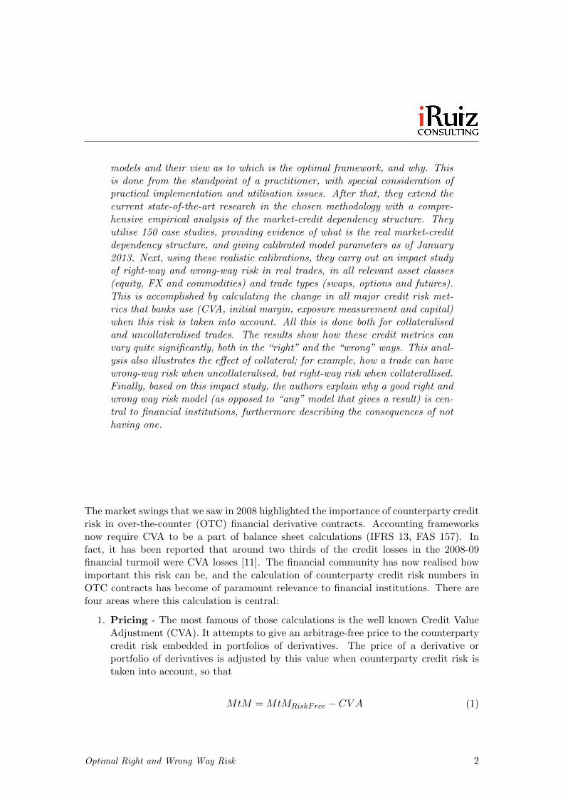
3. Exposure Management - A well-established way to manage the credit risk thatan institution has to a given counterparty is by setting credit exposure limits.Typically, these limits are set to a Potential Future Exposure (PFE)3 risk metricat a given confidence level (e.g. 95%). This limit-setting technique is also used inmarket risk, but with a short time horizon (e.g. 10 days). A counterparty maydefault quite far in the future, and so credit risk limits must have a time-profilecomponent, that must go as far as the maturity of the portfolio of trades withthat counterparty. The size of the limit is a reflection of the credit standing ofthe counterparty, the expectd Loss Given Default and the specific risk appetite ofthe financial institution to that particular firm. Typically, if the PFE metric fora given counterparty breaches its limit, that breach is recorded, it is investigatedand then it is either justified or the trading desk that caused it is forced to bringthe PFE profile down, either by unwinding trades or by booking new offsettingtrades. An illustration of this PFE and limit set up can be seen in figure 1.
0 1 2 3 4 5 6 7 8 9 100
50
100
150
years
$
PFE 90%
Limit
Figure 1: Illustrative example of PFE profile and PFE limit for a counterpaty.
4. Initial Margin - In order to mitigate counterparty risk, both sides of a financialagreement can enter into a collateral agreement by which the counterparty withpositive credit exposure can receive some securities (e.g. cash, bonds, etc) to bringdown the net exposure. Sometimes, the counterparty with the stronger credit
3PFE at a given (X) confidence level is the X-th percentile of the possible values of the portfolio of
trades, floored at zero; ie, X =(∫ PFEX,t
−∞ Ψt(P ) dP)+
where P is the portfolio price, Ψt(P ) is the
probability distribution of P at the future time point t, (·)+ ≡ max(·, 0) and X is a given confidencelevel.
Optimal Right and Wrong Way Risk 4
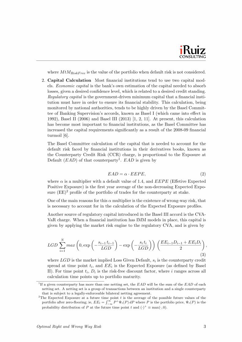
standing may require some collateral in advance, which is set aside as “extra”insurance. Such over-collateralisation is typically done by derivative dealers withhedge funds, or by central clearing houses with derivative dealers. These assets arecommonly referred to as Initial Margin (IM) or Independent Ammount. Typically,this IM is calculated as the maximum exposure at a high confidence level (e.g.99%) that the strong counterparty may have to the weaker one during the live ofthe trade; in other words, the IM will be the maximum of the PFE profile at thechosen confidence level during the life of the trade.
Figure 2: Illustrative example of Initial Margin calculation.
How right and wrong way risk appears
When calculating any credit exposure metric, like the EEt or PFEt profiles, we need tomeasure exposure at default. The “at” is a subtle but crucial concept. When we say,for example, that PFE at 90% confidence in one year is $1m, we are saying that “in90% of the potential future scenarios in which the counterparty defaults in one year, ourexposure to it will be lower then $1m”, as opposed to “in 90% of the potential futurescenarios in one year, our exposure to it will be lower then $1m”. From a mathematicalstandpoint, to model the former case we need to build a dependency structure betweenpotential counterparty default events and the portfolio value. When this dependency isnon-neglegible, it is often said that there exists a “market-credit” dependency4.
4Furthermore, this is often referred to as “market-credit” correlation, but the reader should bear inmind that is a language simplification, as correlation is only one basic measure of dependency. Ingeneral, we are interested in the dependency structure, which will have a correlation factor reflectingthe linear interdependency of the factors at stake, but that can be oversimplified if we refer to it onlyas a correlation effect. We are going to see later how this oversimplification can lead to exposure
Optimal Right and Wrong Way Risk 5
When this dependency is such that the exposure increases with the probability of default,it is said that we have positive dependency. In these cases, the structure of the trade“exacerbates” the credit risk embedded in it, and hence it is said that we have wrong-wayrisk (WWR). However, when it works the other way round, that is when the exposuredecreases as the default probability increases, it is usually said that we have negativedependency, and this effect is called right-Way risk (RWR), since the size of the creditrisk decreases as the counterparty approaches a potential default.
For a number of historical reason it is common to focus on wrong-way risk only. The“other side of the coin”, right-way risk, is often somewhat forgotten5. It is howeverimportant to realise that both exist, and a financial institution should have a set upthat encourages the creation of RWR. We are going to see in later examples how botheffects are equally important. For simplification, we shall refer to the joint effect ofmarket-credit dependency that creates either RWR and WWR as “directional-way risk”(DWR), as they only are two sides of the same coin.
This DWR effect appears mainly in four asset classes: equity, foreign exchange (FX),commodities and credit. This is best explained with a number of examples:
• Equity - As an example of WWR, let’s say we buy a put option from a coun-terparty with its own stock as the option reference entity. In the event of thecounterparty defaulting, we know that the value of the stock will be zero (or veryclose to zero) and hence the option value will be maximum. An example of RWRwould be its complementary call option, as in the event of default we know thatthe value of the option would be zero.
• Foreign Exchange - Suppose that we are a solid institution in a mature econ-omy and we enter a cross-currency agreement with an institution in an emergingeconomy; this could be the central bank, a commercial bank or other commercialfirms. In this agreement, we receive the “mature” economy currency and pay the“developing” economy currency. In the event that the counterparty is under creditdistress, chances are that its currency will be suffering a devaluation and thus thevalue of the transaction for the solid institution should increase substantially. Asa result, we shall observe that as the counterparty’s default probability increases,it may owe more and more to us. This is WWR.
• Commodities - There are lots of companies whose financial performance dependson the price of some commodities. This includes commodity producers as well asbusinesses where an important source of cost are commodity prices. For example,an oil producer may decide to synthetically sell in advance part of its productionby shorting oil futures. As a result, the dealer at the other side of the transactionwill be long those futures. In the event of a strong collapse in the price of oil, the oil
miss-calculations.5In the authors’ opinion, this is because this effect was initially brought to the attention of financial
institutions by the Basel Committee, which focuses principally on the “negative” side of risk, whichis WWR in this case.
Optimal Right and Wrong Way Risk 6
producer may enter into financial stress and its default probability may increase,but from the dealer’s perspective of counterparty credit risk this is good, as in thiscase the oil producer will not owe anything to the bank. This is an example ofRWR.
• Credit - The credit asset class offers very good example of WWR. Suppose thatwe buy protection on Bank A, via a CDS contract. We buy this protection froma Bank B that shares a common business and economic environment with BankA. It is quite likely that if the counterparty (Bank B) approaches default or goesinto liquidation, the CDS originally bought will be well in-the-money and so mypotential loss from this CDS can be very high.
Specific and General DWR
There is another important concept that is widely used when dealing with this topic:“specific” Vs “general” DWR. A transaction is said to have specific DWR when thedependency between a default event and the transaction value is absolute. An examplecan be seen when we buy a put option from a counterparty on its own stock. In the eventof the counterparty defaulting, we know for sure that the value of the option will be itsfull nominal amount. However, when the dependency comes through general economicfactors, then we have general DWR. An example can be when we buy a put optionfrom a counterparty with a stock as reference entity that is highly dependent with thecounterparty’s stock price. In that case, it is likely that the value of the option will behigh if the counterparty defaults but it is not guaranteed and the value of the option inthat event is not certain in advance.
The reader should note that, in the case of specific DWR, we do not require any model.This is because, as previously stated, when we measure exposure, we always measure itsubject to default and, in the case of specfic DWR, we know with certainty the value ofthe exposure in the event of couterparty default. In fact, the Basel Committee recognisesthis through its CCR capital charge: “the instruments [. . . ] for which specific wrong wayrisk has been identified are not considered in the same netting sets as other transactionswith the counterparty”; in such cases the models must be set up so that “EAD equalsthe value of the transaction under the assumption of jump-to-default” [11].
However, in the case of general DWR, a model is needed because the exposure valuesubject to default cannot be predetermined; it is a stochastic variable.
A very special case that is a hybrid between those two can be seen in collateralised FXtransactions when the counterparty is either a sovereign or a very big counterparty (eg,a state-owned company that runs a monopoy) in an emerging economy, as in those casesthe counterparty default will trigger a special dislocation of the market. We can see itas an hybrid between the specific and the general DWR cases as we do not know forsure the potential credit loss, but we can have a priory a good idea of what to expect in
Optimal Right and Wrong Way Risk 7
the event of default6.
Key elements of an optimal DWR model
There are a number of characteristics that an optimal DWR framework should have inthe authors’ view:
Model Adequacy Models are mathematical tools that aim to describe some aspect ofreality. As a consequence, models must be driven by real data as much as possible. Thisis as opposed to pre-conceptions as to how should things behave. In this way our modelswill be more likely to describe the actuality of things, and hence will capture better thetrue economic risks.
These models must also be as simple as possible. By designing simple models, imple-mentation and maintenance becomes easier, faster and more economical, and model riskis minimized. In this way we may increase the ease of communication of model detailsin the organisation, as well as subsequent model usage.
In the author’s view, the Quant community has a track record of making these twomistakes, that should be avoided in the future.
Data Driven Calibration A model is not only a set of equations, but also a calibrat-ing methodology. This is quite important, since a “good” model that is not easy tocalibrate, that has a large calibration error or uncertainty, or that has a strong degreeof subjectivity in the calibration, has limited value in capturing true potential hiddenrisks.
Minimal Impact in existing systems All financials institutions already have in placea calculation framework for counterparty credit risk metrics. The approach consideredto be the most advanced is the Monte Carlo simulation. An optimal DWR modelshould leverage as much as possible from an existing platform, so that a transition to aframework with DWR is straightforward to manage and, also, economical.
6Let’s say that we have we have a cross currency swap with an emerging market (EM) government,that is fully and symmetrically collateralised. Because of that, the only credit risk that we have is theclose-out risk, also known as “gap” risk. The key special feature of this type of trade is that, as datashows (Asian crisis, Russia, Argentina, etc), there tends to be a big devaluation jump immediatelyafter default. For this reason, if we are long the EM currency in the defaulted trade, for example,our naked market hedges are short that currency, hence those hedges should provide a positive profitafter default, and so the real credit risk is quite small. If we are short the EM currency in the trade,the opposite happens. This is specially important in collateralised facilities as in those cases we arehighly sensitive to short-term market moves. This phenomena is characteristic of FX transactionswith emerging markets; it does not appear in any other asset class or counteparties. The key elementhere is that the counterparty is so important that its default triggers a jump in the FX rate afterdefault.
Optimal Right and Wrong Way Risk 8
Easy understanding by non technical users At the end of the day, in practice, mostpeople concerned with counterparty credit risk in a financial institution have an intuitiveunderstanding of the models, but not of their details. For this reason, if we want a DWRto have a positive and strong impact in an organisation, it must be easy explain to a non-technical audience and avoid overly abstract concepts as much as possible. All inputsto a model must be simple to understand by any user, and changes in results must betractable relative to changes in the input. In the authors’ opinion, this is a centralcharacteristic that models should possess in a commercial environment, and that is alsooften forgotten by the Quant community.
What if we do not have a DWR model?
Correct modelling of both RWR and WWR is of paramount importance to a financialinstitution. First of all, without such model the exposure estimates in the counterpartycredit risk framework will not be correct and hence the institution will be incapableof understanding the true extent of the risks that it is actually carrying. As a result,the pricing and management of counterparty credit risk will contain faults. Secondly,without a DWR model, the institution will not have any tool to encourage trading desksto create RWR when possible and to discourage the creation of WWR; it the authors’view that this should be a fundamental risk management policy.
For these reason, a good DWR model is crucial to a good management of the credit riskthat a financial institution carries in its book of derivatives.
This piece of work
Given how important DWR is, in this paper we are going to answer, in detail:
1. What is the optimal way to model DWR?
2. What is the actual extent of DWR in a financial institution?
3. What happens if DWR is not properly modelled?
4. Do we need to consider both right-way and wrong-way risk?
In order to provide answers to these questions, we will firstly review the existent method-ologies in this area. We will analyse the strengths and weaknesses of each of them, andthereby explore which of them should be considered as the optimal methodology. Nextwe will extend the state-of-the-art research in this “optimal” framework with an empir-ical study of the functional form of the dependency that drives DWR; that is, we aregoing to see how it actually is, as opposed to guess how it is. We will do this with 150cases studies accross all relevant asset classes. Finally, we will study the impact of DWRin an organisation with a number of realistic sample calculations: options, swaps and
Optimal Right and Wrong Way Risk 9
futures, both collateralised and uncollateralised, with real counterparties, with modelscalibrated as of January 2013.
Review of currently available methodologies
To the author’s knowledge, these are the existing fundamental methodologies for DWRmodelling:
1. Basel framework: constant multiplier α, stress testing and stress cali-bration
This is the simplest approach, and it is the one used by the Basel Committee forthe calculation of regulatory capital [1, 11].
In this set up, RWR is not considered; rather, only WWR is taken into considera-tion. WWR is accounted for by increasing the exposure metric by a constant factorα across the board, for all counterparties and nettings sets without any particularconsiderations. By default, α = 1.4. In theory, financial institutions can applyfor a lower α, but it can never be below 1.2 according to the Basel Accord. Someinstitutions have an α greater than 1.4. The drivers of the value of α are “low gran-ularity of counterparties, particularly high exposures to WWR, particularly highcorrelation of market values7 across counterparties and other institution-specificchararteristics” [1]. Estimates of α reported by banks range from 1.07 to 1.10 [7].
Further to this, banks must have operational procedures for the identification ofWWR [1]. The Basel II accord does not give much details as to how to do this.Financial institutions and local regulators have typically interpreted this by settingup a stress testing framework to monitor the WWR carried in their portfolios.
However, in Basel III it is given much more attention. To further address thematter, the Committee provides (i) a more detailed description of the operationalprocedures of stress testing, (ii) indicates how to treat trades where specific WWRis identifiend and (iii) asks financial institutions to calibrate the exposure modelsboth as normally done and to stress credit conditions for the portfolio of counter-parties, so that the calibration to be used for the capital calculation should be theone that delivers the highest capital number [11].
2. Change of risk measure in RFE model
Cesari et al. [4] and Iacono [8] propose to change the risk measure in the RiskFactor Evolution (RFE)8 models that drive the exposure calculations. In a risk-neutral framework, a change in a risk measure can be translated to a change in the
7The authors deem that by “market values”, the same is meant as what we call here “exposures”8By RFE models it is meant all the models of market factors (e.g. interest rates, FX rates, equity
prices, commodity prices, implied volatilities, credit, etc) that drive the exposure metrics.
Optimal Right and Wrong Way Risk 10
drift of the RFE models9. Hence, using the example of the oil producer discussedabove, if we know that the exposure subject to default is lower than that withno RWR, we can adjust the drift of the oil price in its RFE model to obtain thedesired effect at the exposure metric.
3. Brute force approach
This methodology is impractical as it requires too much computational power, butit is good to understand it as it naturally leads to the next methodology type.
Suppose that we have a default stochastic model in our suit of RFE models thatcan be used to simulate defaults in our counterparties. Also, let’s say that thatmodel has some sort of dependency structure with all other market factors (e.g.equity prices, FX rates, commodity prices, credit spreads).
Suppose also that in our Monte Carlo (MC) engine for the calculation of the expo-sure metrics profiles (EEt, PFEt) we use N scenarios. In that MC engine, whatwe want to measure are exposure metrics subject to default; hence we are inter-est only in those market scenarios where the counterparty at stake has defaulted.Given that we need N of those scenarios10, we can run the RFE models iterativelymany times, more than N times for sure, and we can then disregard those scenarioswhere the counterparty has not defaulted and pick, for the calculation, those wherea default has occurred. We can do this iteratively until we obtain the desired Nscenarios of risk factors where a default has occurred. If we use these scenarios forthe exposure profiles, we are measuring exposure metrics subject to counterpartydefault, as desired.
An alternative to this method, that is more computationally efficient, is to generatefirst a set of market factors, N scenarios, without considering any counterpartydefaults. Then we can carry out in each scenario a stream of M default simulationsconditional on the market factors of each particular scenario. In this way, ineach MC time step, we will have N market scenarios and M default simulationsper market scenario. Essentially, we are adding a new “counterparty default”dimension to each scenario. Then, if scenario i has mi defaults, we can give adefault weight wi to each scenario that will be taken into account when calculatingthe exposure metrics. In the limit when N and M are large, this gives the sameresult as the methodology of the previous paragraph.
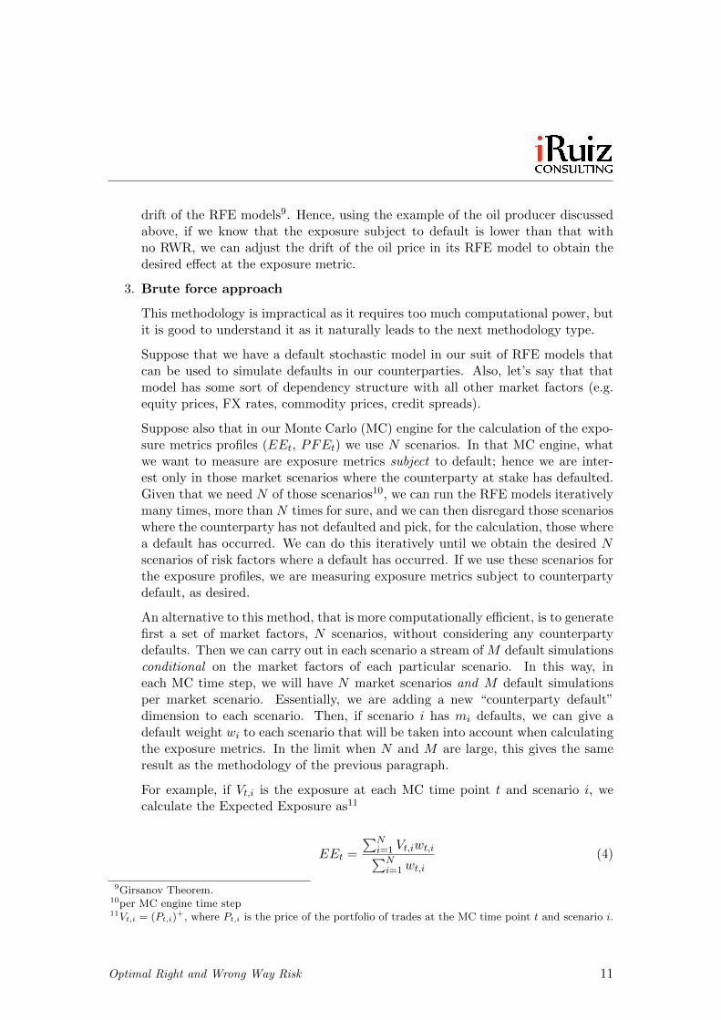
For example, if Vt,i is the exposure at each MC time point t and scenario i, wecalculate the Expected Exposure as11
EEt =
∑Ni=1 Vt,iwt,i∑Ni=1wt,i
(4)
9Girsanov Theorem.10per MC engine time step11Vt,i = (Pt,i)
+, where Pt,i is the price of the portfolio of trades at the MC time point t and scenario i.
Optimal Right and Wrong Way Risk 11
wt,i =mt,i
M(5)
4. Change of risk measure in exposure metric calculation
Equations 4 and 5 provide a numerical way to perform a change in the risk weightof each scenario in a MC simulation, in order to account for DWR. However, if wehad an analytical expression for the default probability subject to a given set ofmarket factors scenario, there would be no need to do the M default simulations.Instead, a fast analytical operation could calculate each wt,i and we will only needthe N market factor scenarios per MC time point.
The reader should note that this methodology is no more than a change in riskmeasure, implemented when the exposure metric calculations are performed. Thatis, we start with a distribution of exposures where no default information existΨ(V ) and we transform it to another distribution Ψ′(V ) where default in accountedfor. In this sense, the operator that transforms Ψ(V ) into Ψ′(V ) can be seen as aRadon-Nikodym derivative [4].
There are three ways that have been proposed to do this:
Merton Model approach Cespedes et al. [5], D. Rosen & D. Saunders [12] andCesari et al. [4] propose a Merton model for this change of risk measure, using anAsymptotic Single Risk Factor (ASRF) model for the dependency structure. Thismodel has the following key components.
• Firstly, in this framework we say that the credit worthiness of a counterpartyis dictated by a latent variable Y . This variable is then decomposed intoa systematic (Z) and idiosyncratic (ε) components with a correlation ρ asfollows:
Y = ρZ +√
1− ρ2 ε (6)
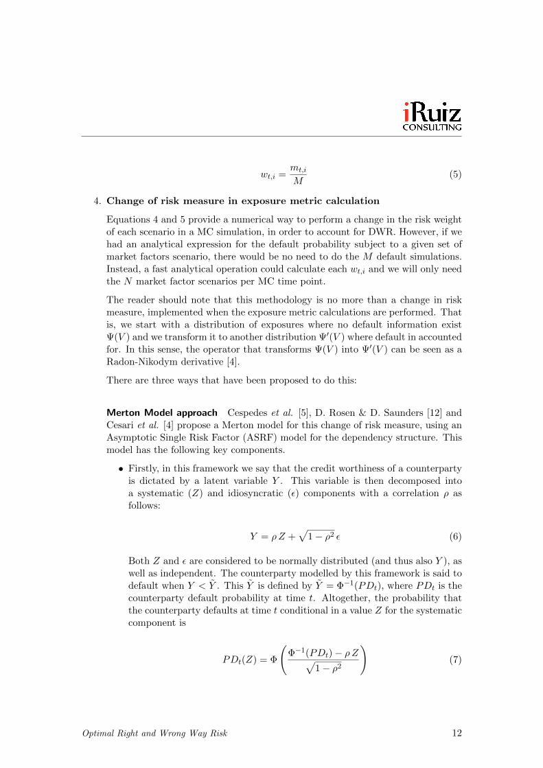
Both Z and ε are considered to be normally distributed (and thus also Y ), aswell as independent. The counterparty modelled by this framework is said todefault when Y < Y . This Y is defined by Y = Φ−1(PDt), where PDt is thecounterparty default probability at time t. Altogether, the probability thatthe counterparty defaults at time t conditional in a value Z for the systematiccomponent is
PDt(Z) = Φ
(Φ−1(PDt)− ρZ√
1− ρ2
)(7)
Optimal Right and Wrong Way Risk 12
• Secondly, at a given future time point t, the exposure values (V ) to a givencounterparty will follow a certain empirical distribution density f(V ) and acorresponding cumulative density function F (V ). By constrution, F (V ) isa uniform distribution, and can be mapped to a ”market” factor X that isnormally distributed as
X = Φ−1 (F (V )) . (8)
• Thirdly, in this modelling framework X represents the market variable, and Ythe credit variable of the counterparty; we need to state the dependency struc-ture between them. There are two versions of this in the literature:Cespedeset al. and D. Rosen & D. Saunders link the market variable X and the de-fault latent variable Y with a joint normal distribution function with a givencorrelation r. Cesari et al. state that X ≡ Y . In the former case, the depen-dency structure between the market factor X and the latent variable Y is abivariate normal distribution with correlation β = r · ρ, In the later case thatdependency structure also follows a bivariate normal distribution but with acorrelation β = ρ.
Given this theoretical framework, we can proceed as follows to calculate the sce-nario weights wt,i. At a given time point t, scenario i will have a value for theexposure Vt,i, from which we can calculate its corresponding Xt,i using equation8. Then, we either generate a corresponding Zt,i using the binormal distributionfunction with correlation r, or we simply state that Zt,i = Xt,i. Once we have Zt,i,we calculate the default probability in this given scenario and time point usingequation 7. The weight for that scenario and time step is wt,i = PD(Zt,i). If weproceed like this for every scenario and time step, we can attach a weight to eachof them, hence transforming Ψ(V ) into Ψ′(V ).
As a final remark, the reader should note that both versions of this methodologyshown here are equivalent. We have indicated that the former version can bereduced to a single bivariate normal distribution with a correlation β = r ·ρ. Sinceboth r and ρ are non-observable variables, what really matters is β (which is alsoan unobservable variable). As a result, both versions are the same with the onlydifference that one of them further decomposes the β into two further parameters.
This modelling framework has been used in the literature to give estimates of theα parameter used in the Basel Committee framework for capital calculation, givingvalues for α that range from 0.89 to 1.27 [5].
Empirical Analysis approach The second version of this type of models has beenproposed by Ruiz [13] and Hull & White [7]. In this modelling framework, thefunctional form that determines the dependency between the market factors and
Optimal Right and Wrong Way Risk 13
the default events is given by empirical data, as opposed to latent non-observablevariables.
Suppose that we find a market factor ‘x’ so that the default probability of a coun-terparty can be expressed in the form
PD = g(x) + σ ε, (9)
where ε is a normalised random number that can follow, in principle, any distri-bution. We use the variable ‘x’ to denote the DWR driving market factor. Thisfactor could be an equity price, an FX rate, a commodity price, or any marketvariable in which we observe a relationship as described by equation 9. If the MCsimulation that is used to compute the counterparty credit risk metrics alreadycontains a simulation for x, with a given dependency structure to all other marketfactors, then we can use those values of x in each scenario to obtain the necessaryinformation for the default probability for that counterparty in that scenario andtime point, and hence of the weight wt,i. In other words, we can say that
wt,i = g(xt,i) + σ ε. (10)
In this framework, the task of the researcher is to discover the best DWR drivingfactor and optimal functional form for equation 9.
For example, it has been observed that an equity price could be used as the marketfactor x, and equation 9 could be calibrated using the default information embed-ded in the credit spreads; Ruiz [13] showed with one illustrative example (Ford)how a functional form g(x) = AxB could be an optimal candidate for this purpose.
Portfolio Value approach The third and final version has been proposed by Hull& White [7]. In it, the researcher estimates the default probability, and hence thescenario weight wt,i using a functional form like
wt,i = h(Pt,i) + σ ε, (11)
where Pt,i is the price of the portfolio of OTC derivatives with the counterparty atstake. In this case, the market factor that drives the dependency structure with thedefault probability is not an actual market risk factor, but the price of a portfolioof trades. Hull & White show a number of numerical results in this framework inthe context of CVA pricing [7].
5. Stressed Scenario
Optimal Right and Wrong Way Risk 14
Mihail Turlakov [14] has recently proposed a model that is based in a marketstressed scenario of the counterparty’s government default, so that the EE profilewith DWR is a combination of the stressed and unstressed EE profiles.
The idea is based in three key points. Firstly, we need to postulate what will bethe impact in the markets of the counterparty’s sovereign default (eg, if the Koreangovernment defaults in its debt, the KRWUSD exhange rate will drop by 30%).We then calculate the EE profile of the book of trades under consideration withthat stressed market scenario as a starting point. If the portfolio contains WWR,this new stressed EE will be higher than the standard one.
Secondly, “since the major market dislocation is given by the situation of thesovereign defaulting as well [as the counterparty]”, the actual EE of the portofoliowill be given by a combination of those two stressed and unstressed EE profiles,with the default probability of the sovereign defaulting conditional of the counter-party having defaulted as the weight between them:
EEDWR = P (sov|cpty)EEstress + (1− P (sov|cpty))EE (12)
Thirdly, we say that the default probability of the the sovereign conditional onthe counterparty having defaulted is λ times the sovereign default probability:P (sov|cpty) = λP (sov)
All this, together with some simple smooth interpolation assumptions lead to aDWR expected exposure profile given by
EEDWR = EE + λP (sov) (EEstress − EE)
(1− tanh
(P (sov)
Pthres
)), (13)
where Pthres is “a near default or half-live threshold marking the crossover betweenthe two extremes”.
Critique and Preferred Model
The previous section has demonstrated the basic methodological types existent for DWR,to the authors’ knowledge. In this section we shall carry out a critical analysis of them,highlighting our views regarding the strengths and weaknesses for each of them. Thiswill be done from the standpoint of a practitioner, considering that a good model isnot only a mathematical framework, but also a calibration methodology that shouldbe as objective as possible. It should furthermore be easy to implement and to fastrun calculations. It should meet the current demands for risk models, which are beingstrongly driven by risk management and capital calculation, and hence back-testing isof great importance.
Optimal Right and Wrong Way Risk 15
Basel framework The first methodology, which is based on a constant multiplier α,stress testing and stress calibration, can be seen as the most simple approach, as itprovides the same constant shock to the capital calculation regardless of the counterpartyand the actual book of trades in its portfolio. The most positive side of this method isthat it is very simple to implement and understand. On the negative side, first of all, itdoes not provide any insight into the true DWR that an institution is carrying. Secondly,it does not provide any incentive to the dealing desks in a financial institution to createRWR, or to avoid WWR, which should be one of the key elements for an optimal DWRstrategy12.
Change of risk measure in RFE model The positive aspect of this methodology is theease with which it can be implemented: all that is required is to change the drifts inthe calibration and run the calculations as usual. On the other hand, the practitionerwill have to face the question of “how much should I change the drift”? There is noway to answer that question in a proper way, and so the practitioner will have to assessexternally, in a qualitative and subjective way, whether the book of trades has RWR orWWR. This is straightforward to do for a single trade, but it can become quite difficult, ifnot impossible, when the book contains a few hundreds or thousands of trades. Secondly,even if that is achieved, it is not clear how much change in the drift is needed; it appearsthat in practice, the calibration of the extra drift needed to reflect the DWR would bea “guestimate” at best. Also, it adds some extra computational demands that couldnot be negligible, since this drift change would be specific to each counterparty, as eachwould have different DWR requirements, and thus it would be necessary to create adifferent set of market factor simulations for each of them.
Brute force approach Provided that we have a good model for the market-credit de-pendency, the “brute force approach” seems to offer, in principle, a better framework
12To overcome this problem, banks are asked to have in place operational procedures to identify WWR;this is definitely better than nothing but, by itself, it will always fail to quantify the actual size ofthe exisiting WWR and it does not tend to provide incentives to the dealing desks in banks. RWRis ignored, and this stress-testing framework is almost always too detached from the dealing desks toprovide any sort of incentive. Having somewhat acknowledged the weakness of this framework, theBasel III accord asked banks additionally to calibrate their counterparty credit risk capital modelsagainst a period of credit stress, and pick for the capital calculation the calibration that gives highestcapital. Again, the authors think that this is suboptimal because the volatilities and other riskparameters that drive the capital calculation will typically be higher in the stress calibration comparedto the standard calibration, and so the Expeced Exposure profiles will tend to be “bumped” up, butthere is no information whatsoever in this calculation about the true DWR carried in the books. Thatis, it simply produces an increase in the exposure profiles, and nothing more. DWR is not modelledat all; for example, if a bank is long a call option where the reference entity and the counterparty arehighly positively dependent (RWR trade), this framework will increase the exposure when in reality,it should decrease it. Also, again there is no encouragement to the dealing desks to create RWR andto avoid WWR. Finally, this framework has been designed for capital calculation at the full bankportfolio level, but there is nothing in it that makes it appropriate for for CVA pricing, exposuremanagement or initial margin calculations.
Optimal Right and Wrong Way Risk 16
to measure and manage DWR. However, it unfortunately requires so much computatingpower that it becomes highly impractical. For example, suppose that we are trying tomeasure WWR in a counterparty with an annual default probability of 1%. If our MCsimulation is calculating the default probability over a time step of one week, the defaultprobability over that period will be approximately 0.02%. This means that, in average,we will have to generate 5,000 default simulations to obtain one desired default event.As a result, the number of simulations N ·M will explode. This is clearly suboptimal.The second version proposed, in which default events are simulated conditionally on aset of values for the market factor, should improve this situation compared to the firstversion, though it will also be too computationally demanding in most cases.
Change of risk measure in exposure metric calculation This modelling approach hasthree versions.
From the modelling adequacy stand point, none of these versions is too complicatedfrom a mathematical perspective. Mostly, all that they add to the existing algorithmsis a routine to calculate the risk weight of each scenario. The difference between themis how exactly that routine works.
There are a number of fundamental differences between the Merton and the EmpiricalAnalysis approach. Firstly, the variables that drive the dependency in the EmpiricalAnalysis approach are given by market data and observed market behaviour, while inthe Merton approach is given in an un-observable latent variable. Secondly, the depen-dency function in the Empirical Analysis is whatever is seen in the market, very littleassumptions are made, while a bi-normal distribution function gaussian copula is usedin the Merton model. Thirdly, the correlation factor is constant in the Merton model,while it is a function of the market variable (x) in the Empirical Analysis approach asdictated by the market data (see appendix J for more details). In the authors’s view,these differences make the Empirical Analysis version a more realistic and powerful mod-elling framework; too abstract models with unobserved variables should be treated withgreat care when other alternatives exist because they can lead to fundamental miscon-ceptions, as in fact happened with the credit asset class and the popular models used toprice CDOs.
Regarding the Portfolio Value method, the authors think it could be, in principle, a soundand robust methodology, but unfortunately it may be difficult to justify a function h(P )in many cases, very specially when the counterparty is not a financial institution.
The most difficult part of DWR models comes to calibration. Here there is a big dif-ference between the three versions. The Empirical Analysis approach is the only onethat has a robust and objective calibration technique behind it. As we will see in greatdetail in later sections, the model is indeed driven by market data analysis that indi-cates the best functional form for the market-credit dependency embedded in g(x). Bycontrast, the Merton model is based on a number of modelling conveniences that are
Optimal Right and Wrong Way Risk 17
not observed: a copula structure with a correlation parameter that exists only as math-ematical instruments; it will be at least difficult to have it objectively calibrated. As aresult, its calibration will be no better than a guess. In addition, the calibration for thePortfolio Value approach carries, in the authors’ view, a very high degree of subjectivityin the calibration process; assigning a default probability to a counterparty depending onthe value of the book of trades associated with it can be problematic, if indeed possibleat all, specially as those books tend to change on an ongoing basis.
A very positive characteristic of all these versions is that implementation should be quitestraightforward for any financial institution. This is because it leverages an existing MCengine for calculating counterparty credit risk. The only work needed to incorporatethis DWR framework is to add the functionality that assigns a risk weight to each ofthe MC scenarios for each time step, and to modify the function that calculates the riskmetrics (e.g. EPE, PFE) so that in accounts for those weights.
Finally, concerning ease of understanding by non-technical users (a very important com-ponent for a model to be successful in an organisation) the Merton model is widely usedin the industry, which is a clear positive. The authors think that the “Empirical Anal-ysis” approach should be easy to explain and understand for non-technical users, sinceit is wholly based on empirical data, as will be shown in later sections. In our view, thePortfolio Value approach is the weakest of the lot, given the high degree of subjectivityin its calibration.
Stressed Scenario In the author’s view, the best characteristic of this method is itssimplicity, it should be quite straight forward to implement, and easy to understand toofor non-technical users. The negatives seem to come, again, from its calibration, as wewill have to “guesstimate” the impact of a sovereign default in the markets, as well asthe λ parameter.
Conclusion In our view, the optimal modelling framework for DWR is the EmpiricalAnalysis. We consider the following characteristics key to its success:
1. The mathematical framework is simple and corresponds best to observed marketbehaviour. The dependency structure used is that seen in the market, which everit is, and no un-observable variables need to be created.
2. Its calibration is robust, based on empirical data, and it is independent of the bookof trades with a given counterparty. Moreover, it has no subjective component.
3. Its implementation will leverage strongly from an already existing MC engine forcounterparty credit risk calculations; it does not need to new market scenarios orderivative pricing.
4. Given that it is based on empirical data, and that it does not use abstract unob-servable variables or parameters, it is easy to illustrate its fundamentals to non-
Optimal Right and Wrong Way Risk 18
technical users.
In our view, there is nothing as practical, robust and strong as real data to drive a modelthat is used to price and calculate risk. For that reason, we think that the “EmpiricalAnalysis” approach is the optimal one to model DWR13.
Empirical Study
It this section we are going to study actual data with the aim of finding empiricaldependencies that will subsequently deliver a realistic and easily-calibrated (i.e. data-driven) DWR framework.
One of the major problems of studying historical default evens is that they happen quiterarely and hence it can be very difficult to obtain data that is statistically significant.This problem is even more acute when trying to find data on defaults with a DWRcomponent in it. For this reason, in order to obtain relevant information for our purposes,it may be best to use the market available information about default probabilities thatis embedded in the CDS prices, which are daily traded. In particular, we can takeadvantage of a widely used approximation for the instantaneous default intensity (λ),given by [7]
λ =s
1−RR, (14)
where s is the credit spread and RR is the expected recovery rate on the event of default.In particular, we will use data from the one-year par credit spread as this tenor shouldprovide a good proxy for the market’s view of the short-term default probability and,most impotantly, it is amongst the most liquid tenor points in the CDS market; hencewe should be able to find reasonably good quality data.
We now discuss dependency structures for each of the cases previously layed out.
Our final aim is to approximate the best functional form for g(x) in equation 9. Tothis end, we tried four different forms for g(x); power, exponential, logarithmic andlinear.
g1 = A2 xB2 (15)
g2 = A1eB1 x (16)
g3 = A3 +B3 lnx (17)
g4 = A4 +B4 x (18)
13With the only special exception of FX risk with sovereigns in collateralised facilities in EM economies,where the Stress Scenario is able to deal arguably getter with the jump effects that a default cancauses in the market.
Optimal Right and Wrong Way Risk 19
We used a least-squared liner regression method to estimate A and B for each of thosefunctional form gi, using five years of historical weekly data. To assess the relative qualityof each of these fits, we utilised two parameters: the R2 delivered by the regressionand the size of σ, which was obtained as the the standard deviation of {λi − g(xi)}.In principle, we are looking for the fit that delivers the highest R2 and/or the lowestσ.
Equity
For this type of transacions, we want to understand the real (i.e. empirically measured)dependency between a corporate equity price and its probability of default PD. TheMerton model seems to deliver a dependency close to an exponential function (see ap-pendix I), which may or may not be the case with real data. As said, we will obtain thisinformation from the default intensity embedded in its one-year CDS spread.
To do this, we selected a number of representative firms, covering a wide range of regionsand activity sectors. The list of 71 equity prices used can be seen in appendix H.
We give an illustrative example (Societe Generale) of that dependency in figure 3. Allthe results can be found in appendix A. The scatter plots of the default probabilityversus the equity price show a a clear dependency structure between the equity priceand the default probability. As expected, data shows that the lower the equity price, thehigher the market-expected default probability. This can be interpreted in two ways.On one hand, an equity price can be seen as the present value of the expected futuredividends. When a company’s expected future performance becomes compromised, bothits expected future dividends decrease and its probability of not being able to honour itsfuture financial liabilities (i.e., its default probability) increases, hence the observationthat when the equity price decreases its expected default probability increases, and vice-versa. On the other hand, if we see a firm under a Merton model, a decrease in theequity price means a decrease in the value of its “latent assets” and hence, given thatthe debt level is constant, the default probability increases, and vice-versa.
The following table show the values of A, B, R2 and σ2 for the illustrative example(Societe General). The calibration results for all equities studied are shown in theappendix H.
A B R2 σ2
Power 1.1651 −1.5062 77% 5.65 · 10−6
Exponential 3.8569 · 10−2 −5.3928 · 10−2 74% 1.96 · 10−5
Logarithmic −1.0870 · 10−2 4.5231 · 10−2 71% 2.34 · 10−5
Linear −3.132 · 10−2 1.8297 · 10−2 62% 2.48 · 10−5
We can use two methods to decide which of those fits is best. On one hand, if we measurethe quality of the fit by its R2, in 53% of the cases the functional form with the highestR2 was the power law, 27% of the times it was the exponential and 20% times it was
Optimal Right and Wrong Way Risk 20
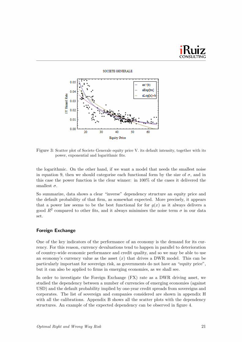
Figure 3: Scatter plot of Societe Generale equity price V. its default intensity, together with itspower, exponential and logarithmic fits.
the logarithmic. On the other hand, if we want a model that needs the smallest noisein equation 9, then we should categorise each functional form by the size of σ, and inthis case the power function is the clear winner: in 100% of the cases it delivered thesmallest σ.
So summarize, data shows a clear “inverse” dependency structure an equity price andthe default probability of that firm, as somewhat expected. More precisely, it appearsthat a power law seems to be the best functional for for g(x) as it always delivers agood R2 compared to other fits, and it always minimises the noise term σ in our dataset.
Foreign Exchange
One of the key indicators of the performance of an economy is the demand for its cur-rency. For this reason, currency devaluations tend to happen in parallel to deteriorationof country-wide economic performance and credit quality, and so we may be able to usean economy’s currency value as the asset (x) that drives a DWR model. This can beparticularly important for sovereign risk, as governments do not have an “equity price”,but it can also be applied to firms in emerging economies, as we shall see.
In order to investigate the Foreign Exchange (FX) rate as a DWR driving asset, westudied the dependency between a number of currencies of emerging economies (againstUSD) and the default probability implied by one-year credit spreads from sovereigns andcorporates. The list of sovereign and companies considered are shown in appendix Hwith all the calibrations. Appendix B shows all the scatter plots with the dependencystructures. An example of the expected dependency can be observed in figure 4.
Optimal Right and Wrong Way Risk 21
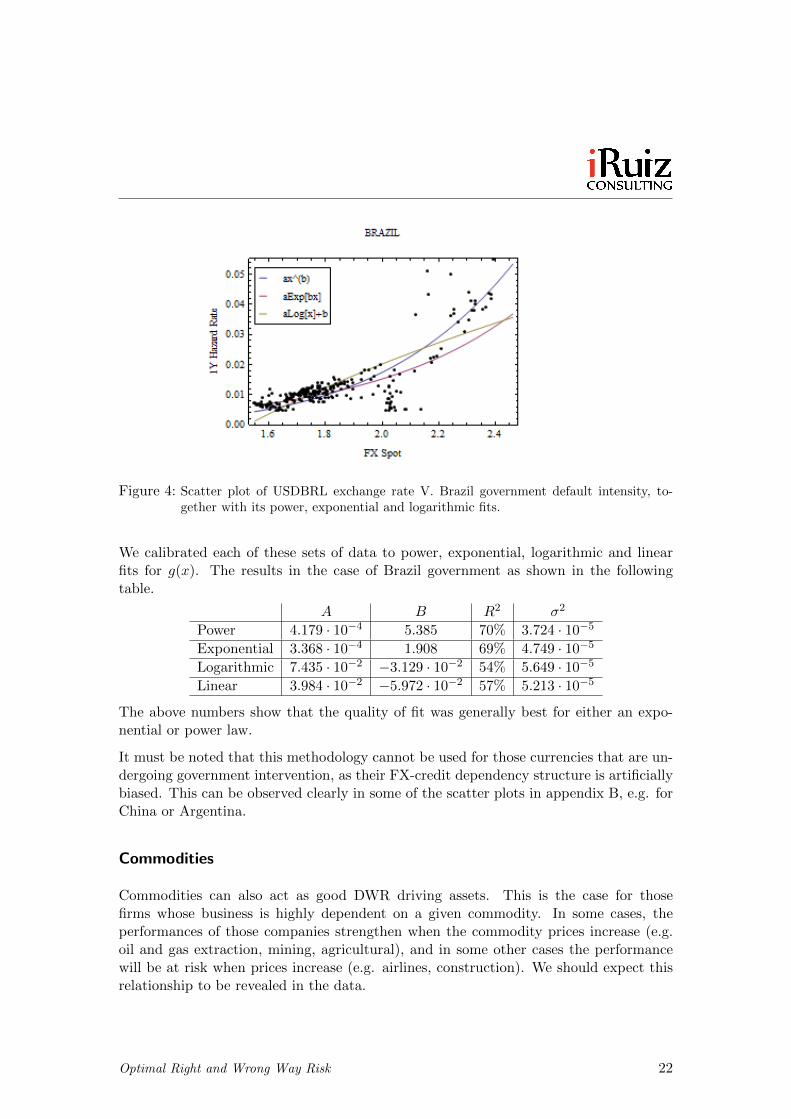
Figure 4: Scatter plot of USDBRL exchange rate V. Brazil government default intensity, to-gether with its power, exponential and logarithmic fits.
We calibrated each of these sets of data to power, exponential, logarithmic and linearfits for g(x). The results in the case of Brazil government as shown in the followingtable.
A B R2 σ2
Power 4.179 · 10−4 5.385 70% 3.724 · 10−5
Exponential 3.368 · 10−4 1.908 69% 4.749 · 10−5
Logarithmic 7.435 · 10−2 −3.129 · 10−2 54% 5.649 · 10−5
Linear 3.984 · 10−2 −5.972 · 10−2 57% 5.213 · 10−5
The above numbers show that the quality of fit was generally best for either an expo-nential or power law.
It must be noted that this methodology cannot be used for those currencies that are un-dergoing government intervention, as their FX-credit dependency structure is artificiallybiased. This can be observed clearly in some of the scatter plots in appendix B, e.g. forChina or Argentina.
Commodities
Commodities can also act as good DWR driving assets. This is the case for thosefirms whose business is highly dependent on a given commodity. In some cases, theperformances of those companies strengthen when the commodity prices increase (e.g.oil and gas extraction, mining, agricultural), and in some other cases the performancewill be at risk when prices increase (e.g. airlines, construction). We should expect thisrelationship to be revealed in the data.
Optimal Right and Wrong Way Risk 22
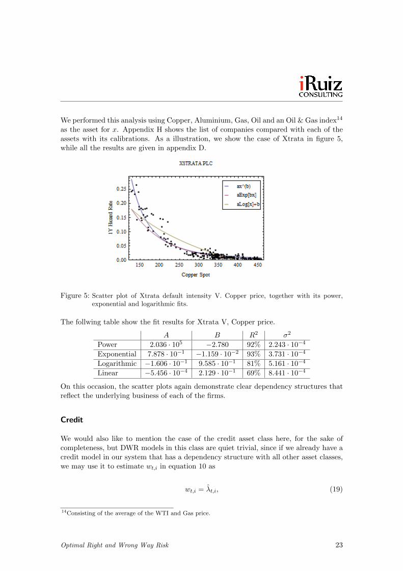
We performed this analysis using Copper, Aluminium, Gas, Oil and an Oil & Gas index14
as the asset for x. Appendix H shows the list of companies compared with each of theassets with its calibrations. As a illustration, we show the case of Xtrata in figure 5,while all the results are given in appendix D.
Figure 5: Scatter plot of Xtrata default intensity V. Copper price, together with its power,exponential and logarithmic fits.
The follwing table show the fit results for Xtrata V, Copper price.
A B R2 σ2
Power 2.036 · 105 −2.780 92% 2.243 · 10−4
Exponential 7.878 · 10−1 −1.159 · 10−2 93% 3.731 · 10−4
Logarithmic −1.606 · 10−1 9.585 · 10−1 81% 5.161 · 10−4
Linear −5.456 · 10−4 2.129 · 10−1 69% 8.441 · 10−4
On this occasion, the scatter plots again demonstrate clear dependency structures thatreflect the underlying business of each of the firms.
Credit
We would also like to mention the case of the credit asset class here, for the sake ofcompleteness, but DWR models in this class are quiet trivial, since if we already have acredit model in our system that has a dependency structure with all other asset classes,we may use it to estimate wt,i in equation 10 as
wt,i = λt,i, (19)
14Consisting of the average of the WTI and Gas price.
Optimal Right and Wrong Way Risk 23
where λt,i represents the model’s short-term default intensity for scenario i at the sim-ulation time t.
More Relationships Found
During the course of this empirical study, we uncovered other interesting data depen-dencies.
European Sovereign Risk
Europe is a special case of sovereign risk, as we cannot use the FX model for the countriesthat are under financial stress (Spain, Portugal, Italy, Greece and Ireland). This isbecause the Euro currency is also being affected by the economic situation of thosemember states that are net creditors within the Euro area. In fact, we tested this andno clear functional form was found between the USD/EUR exchange rate and the defaultintensity of those European countries under stress. These results are given in appendicesE and H.
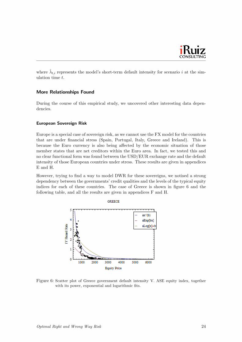
However, trying to find a way to model DWR for these sovereigns, we notised a strongdependency between the governments’ credit qualities and the levels of the typical equityindices for each of these countries. The case of Greece is shown in figure 6 and thefollowing table, and all the results are given in appendices F and H.
Figure 6: Scatter plot of Greece government default intensity V. ASE equity index, togetherwith its power, exponential and logarithmic fits.
Optimal Right and Wrong Way Risk 24
A B R2 σ
Power 4.944 · 105 −1.866 57% 9.400 · 10−1
Exponential 2.440 −1.479 · 10−3 60% 1.516 · 100
Logarithmic −1.509 1.204 · 101 45% 1.193 · 100
Linear −5.310 · 10−4 1.910 · 100 26% 1.618 · 100
This framework seems to provide an excellent way to model DWR with those sovereigns.
Emerging Market Equity
Following up to the above study, we expanded it to emerging economies and explored thelink between the country’s main equity index and the default probability of its sovereigndebt. The results are shown in G and H. We found that there is a clear relationshipthat can be used to model DWR too, and so this can be an effective alternative to usingthe FX rate as the DWR driving asset when, for example, the currency free-floating ismanipulated.
Conclusions of this Empirical Study
The analysis performed illustrates the adequacy of the Empirical Analysis approachto model DWR. It shows several cases where a clear dependency between the defaultintensity can be drawn with a given asset. That asset can be equity prices, FX rates orcommodity prices depending in the nature of the counterparty under study.
We have seen that, for corporates, the equity price appears to be a good candidate forthe DWR driving asset, but not necessarily the only one, as we may be able to use theFX rate or a commodity price as the driving asset too. If more than one is available, itis up to the researcher to decide which is best to use; in fact, a blend of them could beused. We shall expand on this later in the article.
For sovereigns, we have seen that the FX rate of its currency can be a good drivingasset. In the special case of European sovereign risk, or when the FX market is under-goes government intervention, we have seen that we may use the country equity indexinstead.
Regarding the functional form for g(x), we have seen that, from the ones tested, apower-law seems to work quite well, followed by an exponential law. However, there isno reason why a practitioner designing a model for an specific counterparty should notinvestigate other more elaborate forms for g(x).
As a final remark, the authors would like to point out that all these findings can alsobe used outside of the DWR scope. The data shown here imply clear dependencystructures between asset classes (equity-credit, FX-credit, commodity-credit, equity-FX-commodity-credit in emerging market firms, etc.) that go beyond the typical linear
Optimal Right and Wrong Way Risk 25
correlation models, and hence they can (arguably, they should) be used to model thosedependencies in a general framework, even outside of the DWR environment.
Impact of DWR in Counterparty Credit Risk Calculations
So far, we have seen:
• how and where DWR models can be used in a financial institution,
• the different model options available,
• the authors’ view as to the optimal modelling approach in a commercial environ-ment,
• a number of empirically obtained functional forms for the credit-market depen-dency, g(x).
We now wish to understand the impact of DWR in the real world. To do this, werun the preferred modelling framework through a number of sample trades (options,forwards and swaps), with and without a DWR model. When modelled with a DWR,it is realistically calibrated to actual market conditions. We do this for all asset classesthat show a market-credit dependency structure and that subsequently lead to DWR:equities, FX and commodities. We then study the impact of DWR in the CVA, initialmargin, future exposure and regulatory capital calculations.
For CVA, we calculate unidirectional CVA for simplicity. For initial margin, the maxi-mum of the PFE profile at 99% confidence. For exposure management, we use the PFEprofile at 90% confidence, and for regulatory capital, both the EEPE and the regulatoryCS0115 as defined by the Basel Committee.
It is not the goal of this paper to discuss details of collateral modelling, thus we onlyconcern ourselves with an ideal CSA: daily margining, zero threshold, zero minimumtransfer ammount, zero rounding, etc, and a close-out period16 of ten days.
For simplicity, all risk factor evolution models (equity, FX and commodities) operateon one-factor geometric Brownian motion calibrated to the risk-neutral measure as ofJanuary 2013. There is no market for DWR trades, so g(x) cannot be calibrated to amarket-implied measures; it will be calibrated using five years of weekly historical dataas of January 2013. Also, along with Hull & White [7], we have seen that the noise term(σ) in equation 9 did not have any noticeable effect in results, so we are disregarding itin the calculations.
15The version where a IMM compliant market risk VaR engine calculates credit VaR based on parallelshifts of the credit curve.
16Also called Margin Period of Risk by in the context of the Basel Committee.
Optimal Right and Wrong Way Risk 26
A number of simplifications were employed for the RFE diffusion and the derivativespricers, which were seen to have no notable effect on the calculations17.
Some Intuition into the Problem
We said before that right-way risk can be as important as wrong-way-risk and hence ourpreferred term “directional-way-risk” (DWR). We intend to illustrate that point in thissection.
Furthermore, we are going to see in a number of examples that a trade may have wrong-way risk when considered in a collateralised basis, but right-way-risk when considereduncollateralised, and vice-versa. This defeated the original intuition that the we had inthis problem and, it must be said, it took us some time to understand. Thus we deemit worthwhile to dedicate some text to it, in a “pre-emptive” manner; this ought to helpthe reader get the most out of the upcoming examples.
The uncollateralised case is the one that tends to be more popular, and easier to un-derstand, because the exposure that an institution has to a given counterparty is takenas the value of the trades with that counterparty. If that value increases as the defaultprobability of the counterparty increases, we have wrong-way risk, and the exposureprofiles considering this effect should be higher than without it. When the value ofthe trade decreases as the default probability of the counterparty increases, then wehave right-way risk and the exposure profiles should be below those without consideringDWR. The intensity of this effect will be given by the function g(x), as it sets the de-pendency structure between the counterparty default probability and the DWR drivingfactor.
To be more specific, if the price of the trade (or portfolio of trades) is given by P = f(x),the MC simulation that calculates credit metrics will evaluate the trade in every scenariousing that function and, then, when calculating risk metrics like EPE or PFE, it willweigh each scenario by w = g(x). Since g(x) will generally be a monotonic function, thecase for right or wrong way risk is quite straightforward when f(x) is also monotonic.The strength of the DWR will be determined by g(x) and typically the volatility of themarket factor x too, as the higher volatility the more likely that the market factor x willreach points of very high or very low default probability.
The collateralised case is somewhat more subtle. As previously said, we do not wishto focus here on the details of CSA modelling, so we are considering an ideal CSAas described above. In this case, the credit risk profiles will be measured from thedistribution of changes in the 10-day forward price of the trade (or portfolio of trades);
17RFE models are based on geometric Brownian motion with constant volatility. Pricing models areBlack-Scholes for options, risk-neutral valuation for FX forwards and the approximation of continuumpayments for swaps. A single yield curve per currency was used, assumed to be flat and non-stochastic.Implied volatilities are also assumed to be flat and non-stochastic (as the main driver of risk for Black-Scholes options is the underlying spot price).
Optimal Right and Wrong Way Risk 27
that is, the PFE and EPE profiles will be calculated from the distribution, at each pointin time, of changes in the portfolio value over a rolling time horizon of 10 days.
As a result, if P if the value of the netting set under consideration, P = f(x), and if xfollows geometric Brownian motion, we approximately have that
δP ' ∆(x) · δx,
δx ' x · σ ·√
10
260· ε,
where ∆ = ∂f∂x , σ is the volatility of x, and ε is a standard normal deviate. Joining those
two equations, we can say that
δP ' ∆(x) · x · σ ·√
10
260· ε. (20)
This equations provides us with a distribution of δP at at given time point in the future,from which we calculate credit risk profiles like EPE or PFE. In other words, if we arerunning a MC simulation with 10,000 scenarios, at each MC calculation time point wewill have 10,000 value of δP , that come from 10,000 value of xt and 10,000 values ofε.
So far, this does not consider any DWR modelling. When we apply our DWR model tothis distribution, we need to assign a weight to each δP in each scenario. That weightwill come from w = g(x).
In the collateralised case, the exposure measured by the MC simulation in each scenarioand time step is not the value of the portfolio (as it was in the uncollaralised instance),but a realisation of δP as given by equation 20. Hence, the direction of the DWR (either“right” or “wrong”) will be now determined by something different to the uncollatealisedcase: it will be given by a balance between (i) g(x), (ii) ∆(x) and (iii) the geometricnature of δx (i.e., that δP is approximately proportional to x).
For example, suppose that we have a call option, where ∆(x) is a increasingly monotonic,and suppose that g(x) is decreasingly monotonic. Then, the smaller x is before a 10-daymove, the greater its weight w will be on one hand, but on the other hand its ∆(x) willtend to be smaller, an hence δP will tend to be smaller (in absolute value) with it. Onthis way, we could have either right-way or wrong-way risk depending on the balance ofg(x) and ∆(x).
This shows that the direction of the DWR in uncollateralised trades can be different whenconsidered as collateralised, since the drivers of the DWR direction are quite differentto those in the collateralised case.
Optimal Right and Wrong Way Risk 28
The reader may be anticipating from equation 20 a result that we will observe in thenumeric examples: for collateralised trades, if we are long a trade and we have, forexample, RWR, we will tend also to observe RWR when we are short the same trade.This is in contrast to the uncollateralised case, where the direction of the DWR effecttypically gets inverted when switching between long and short in a trade. This is becausethe symmetry in ε in equation 20 when we invert the direction of the trade.
We now proceed with some practical examples.
An FX Forward in an Emerging Market economy
As formerly stated, a source of DWR lies in transactions that are sensitive to FX ratesin emerging economies. This is due to the business nature of firms in these regions, oftenhaving export based economies, which tend to be very sensitive to their FX rates. Thusthe performance of such an economy as a whole, and of individual companies in thoseeconomies, is highly linked to the FX market.
In this example we shall study an FX forward. We are going to see that we can haveeither right-way or wrong-way risk in the uncollateralised case, depending on weatherwe are long or short the trade, but that we will always have wrong-way risk whencollateralised.
Long FX Forward
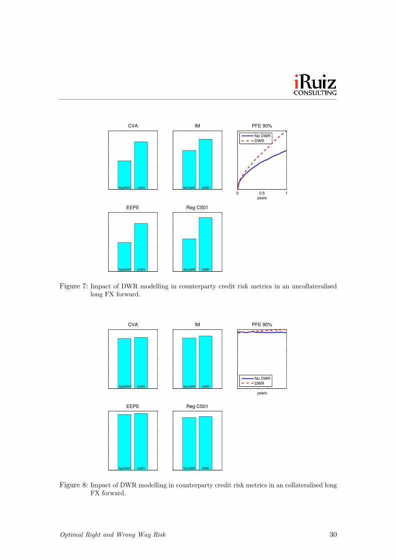
Suppose that we sell to Petrobras, a major oil company in Brazil, a one-year FX forwardon the USD/BRL exhange rate. Data shows a clear dependency between the FX leveland the default intensity of this company best fitted by g(x) = 3.1481 · 10−4 x6.4313,where x is the USDBRL exchange rate (see appendices B and H). Figures 7 and 8 showthe impact of DWR in the counterparty risk metrics, both if the trade is uncollateralised(fig. 7) and collateralised (fig. 8).
In this transaction, we are long the USD/BRL rate. Thus DWR that we have in theuncollateralised case is such that when the BRL devaluates, the default probability ofPetrobras increases and the forward is in-the-money for us; so we have wrong-way risk.This is clearly shown in the PFE-90% profile in figure 7. As a result, all CVA, InitialMargin (IM) and regulatory capital increase most notably compared to its non-DWRvalue.
In the collateralised case, the DWR effect we observe is also wrong-way risk, althoughsmaller this time. This is because (i) the MC paths that carry the most weight w arethose in which USD/BRL is high and (ii) the 10-day changes of the forward, that is adelta-one product, are bigger in those paths with high w (as a result of the geometricnature of the FX rate moves). As a consequence, we have a wrong-way risk effect. This
Optimal Right and Wrong Way Risk 29
CVA
NoDWR DWR
IM
NoDWR DWR
0 0.5 1years
PFE 90%
No DWR
DWR
EEPE
NoDWR DWR
Reg CS01
NoDWR DWR
Figure 7: Impact of DWR modelling in counterparty credit risk metrics in an uncollateralisedlong FX forward.
CVA
NoDWR DWR
IM
NoDWR DWR
years
PFE 90%
No DWR
DWR
EEPE
NoDWR DWR
Reg CS01
NoDWR DWR
Figure 8: Impact of DWR modelling in counterparty credit risk metrics in an collateralised longFX forward.
Optimal Right and Wrong Way Risk 30
effect is small, compared to the uncollateralised case, because exposure is only sensitiveto 10-day moves in the FX rate.
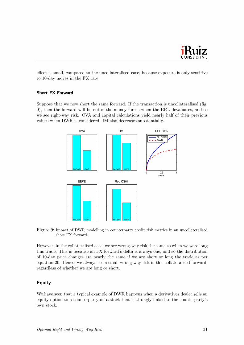
Short FX Forward
Suppose that we now short the same forward. If the transaction is uncollateralised (fig.9), then the forward will be out-of-the-money for us when the BRL devaluates, and sowe see right-way risk. CVA and capital calculations yield nearly half of their previousvalues when DWR is considered. IM also decreases substantially.
CVA
NoDWR DWR
IM
NoDWR DWR
0 0.5 1years
PFE 90%
No DWR
DWR
EEPE
NoDWR DWR
Reg CS01
NoDWR DWR
Figure 9: Impact of DWR modelling in counterparty credit risk metrics in an uncollateralisedshort FX forward.
However, in the collateralised case, we see wrong-way risk the same as when we were longthis trade. This is because an FX forward’s delta is always one, and so the distributionof 10-day price changes are nearly the same if we are short or long the trade as perequation 20. Hence, we always see a small wrong-way risk in this collateralised forward,regardless of whether we are long or short.
Equity
We have seen that a typical example of DWR happens when a derivatives dealer sells anequity option to a counterparty on a stock that is strongly linked to the counterparty’sown stock.
Optimal Right and Wrong Way Risk 31
CVA
NoDWR DWR
IM
NoDWR DWR
years
PFE 90%
No DWR
DWR
EEPE
NoDWR DWR
Reg CS01
NoDWR DWR
Figure 10: Impact of DWR modelling in counterparty credit risk metrics in an collateralisedshort FX forward.
In this section we shall study an example where a put option delivers wrong-way risk,but its complementary call option delivers right-way risk; all in the uncollateralised case.When collateralised, we shall see how the profiles change importantly from a call to aput because of the changes in the profile of the option delta ∆(x).
Long Put Option
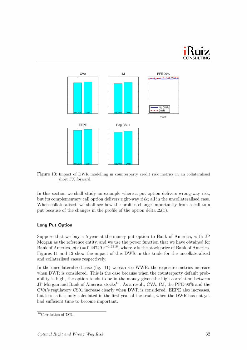
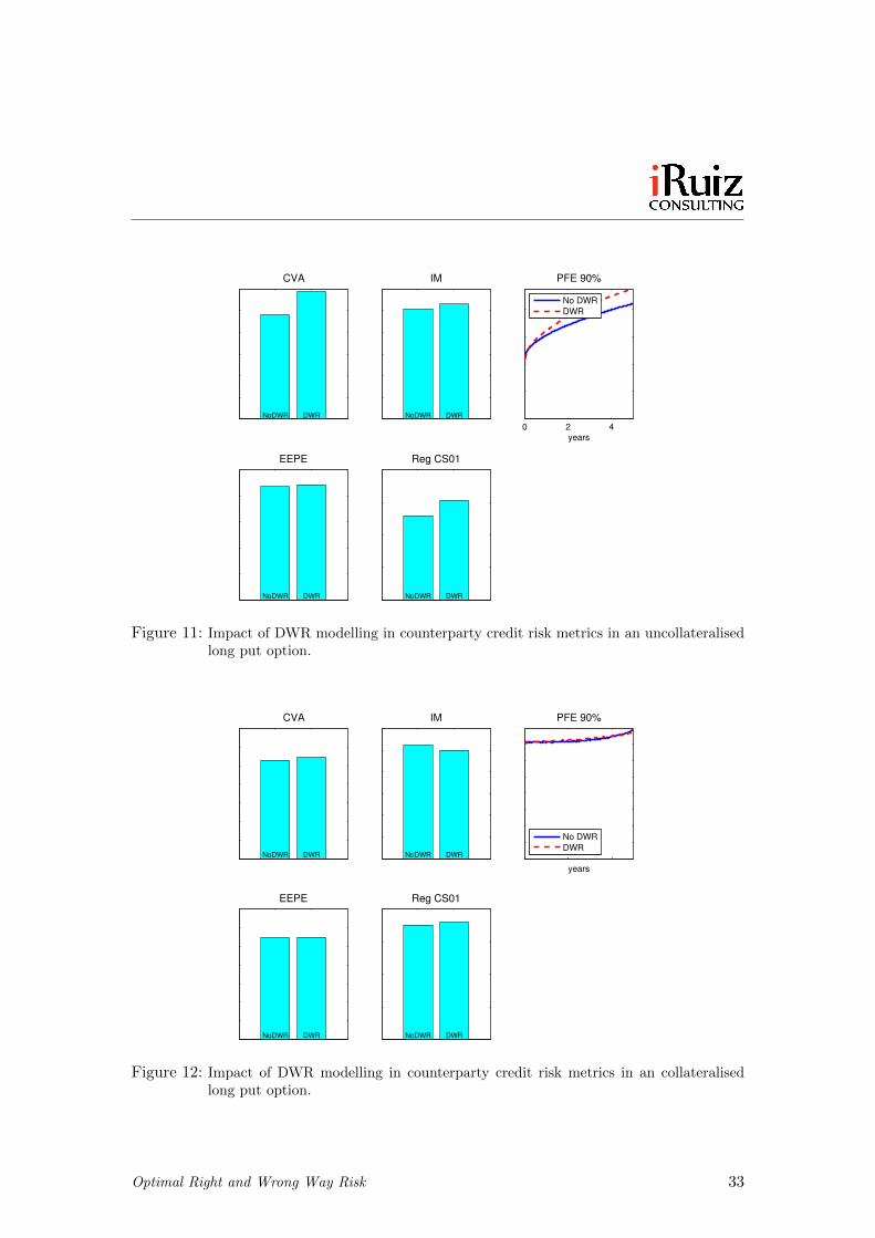
Suppose that we buy a 5-year at-the-money put option to Bank of America, with JPMorgan as the reference entity, and we use the power function that we have obtained forBank of America, g(x) = 0.44749x−1.2216, where x is the stock price of Bank of America.Figures 11 and 12 show the impact of this DWR in this trade for the uncollateralisedand collaterlised cases respectively.
In the uncollateralised case (fig. 11) we can see WWR: the exposure metrics increasewhen DWR is considered. This is the case because when the counterparty default prob-ability is high, the option tends to be in-the-money given the high correlation betweenJP Morgan and Bank of America stocks18. As a result, CVA, IM, the PFE-90% and theCVA’s regulatory CS01 increase clearly when DWR is considered. EEPE also increases,but less as it is only calculated in the first year of the trade, when the DWR has not yethad sufficient time to become important.
18Correlation of 78%.
Optimal Right and Wrong Way Risk 32
CVA
NoDWR DWR
IM
NoDWR DWR
0 2 4years
PFE 90%
EEPE
NoDWR DWR
Reg CS01
NoDWR DWR
No DWR
DWR
Figure 11: Impact of DWR modelling in counterparty credit risk metrics in an uncollateralisedlong put option.
CVA
NoDWR DWR
IM
NoDWR DWR
years
PFE 90%
EEPE
NoDWR DWR
Reg CS01
NoDWR DWR
No DWR
DWR
Figure 12: Impact of DWR modelling in counterparty credit risk metrics in an collateralisedlong put option.
Optimal Right and Wrong Way Risk 33
On the other hand, the collateralised case shows very little sensitivity to DWR effects.This was due to two interacting effects here; a higher weight w as the equity valuedecrease, and a smaller δP as the equity value decrease (due to the geometric diffusionnature of x), seemed to cancel each other out.
In fact, though small in magnitude, we see an interesting effect here: the balance betweenδ(x), g(x), and the geometric nature of δP deliver a small WWR up to four years, whileit then tended to disappear in the fifth year19.
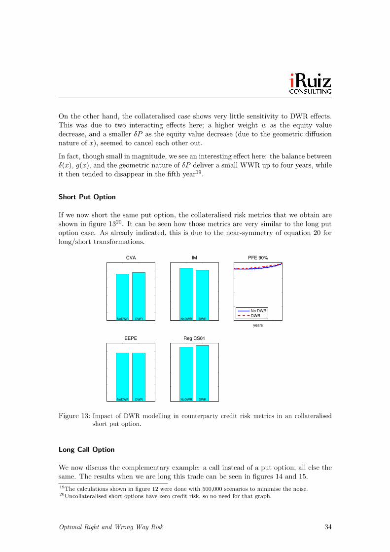
Short Put Option
If we now short the same put option, the collateralised risk metrics that we obtain areshown in figure 1320. It can be seen how those metrics are very similar to the long putoption case. As already indicated, this is due to the near-symmetry of equation 20 forlong/short transformations.
CVA
NoDWR DWR
IM
NoDWR DWR
years
PFE 90%
No DWR
DWR
EEPE
NoDWR DWR
Reg CS01
NoDWR DWR
Figure 13: Impact of DWR modelling in counterparty credit risk metrics in an collateralisedshort put option.
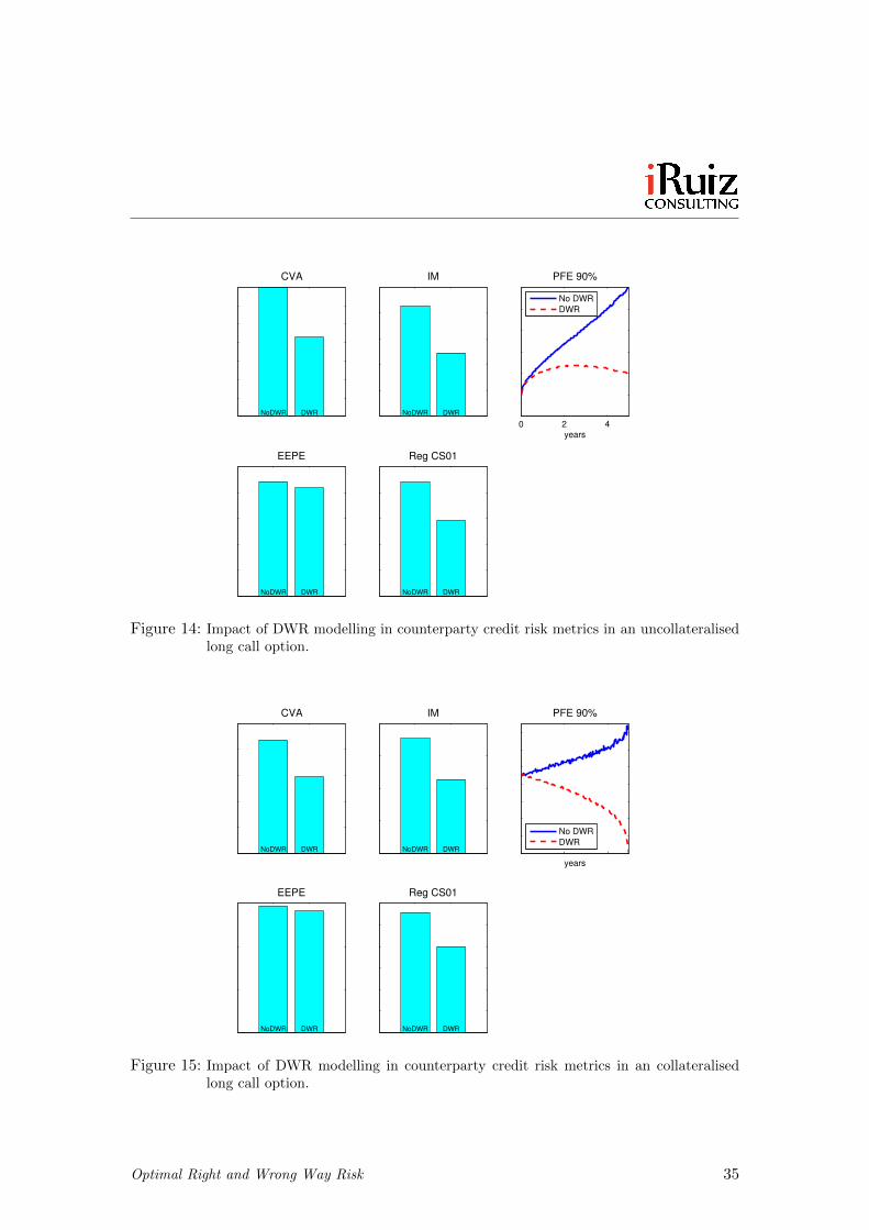
Long Call Option
We now discuss the complementary example: a call instead of a put option, all else thesame. The results when we are long this trade can be seen in figures 14 and 15.
19The calculations shown in figure 12 were done with 500,000 scenarios to minimise the noise.20Uncollateralised short options have zero credit risk, so no need for that graph.
Optimal Right and Wrong Way Risk 34
CVA
NoDWR DWR
IM
NoDWR DWR
0 2 4years
PFE 90%
No DWR
DWR
EEPE
NoDWR DWR
Reg CS01
NoDWR DWR
Figure 14: Impact of DWR modelling in counterparty credit risk metrics in an uncollateralisedlong call option.
CVA
NoDWR DWR
IM
NoDWR DWR
years
PFE 90%
No DWR
DWR
EEPE
NoDWR DWR
Reg CS01
NoDWR DWR
Figure 15: Impact of DWR modelling in counterparty credit risk metrics in an collateralisedlong call option.
Optimal Right and Wrong Way Risk 35
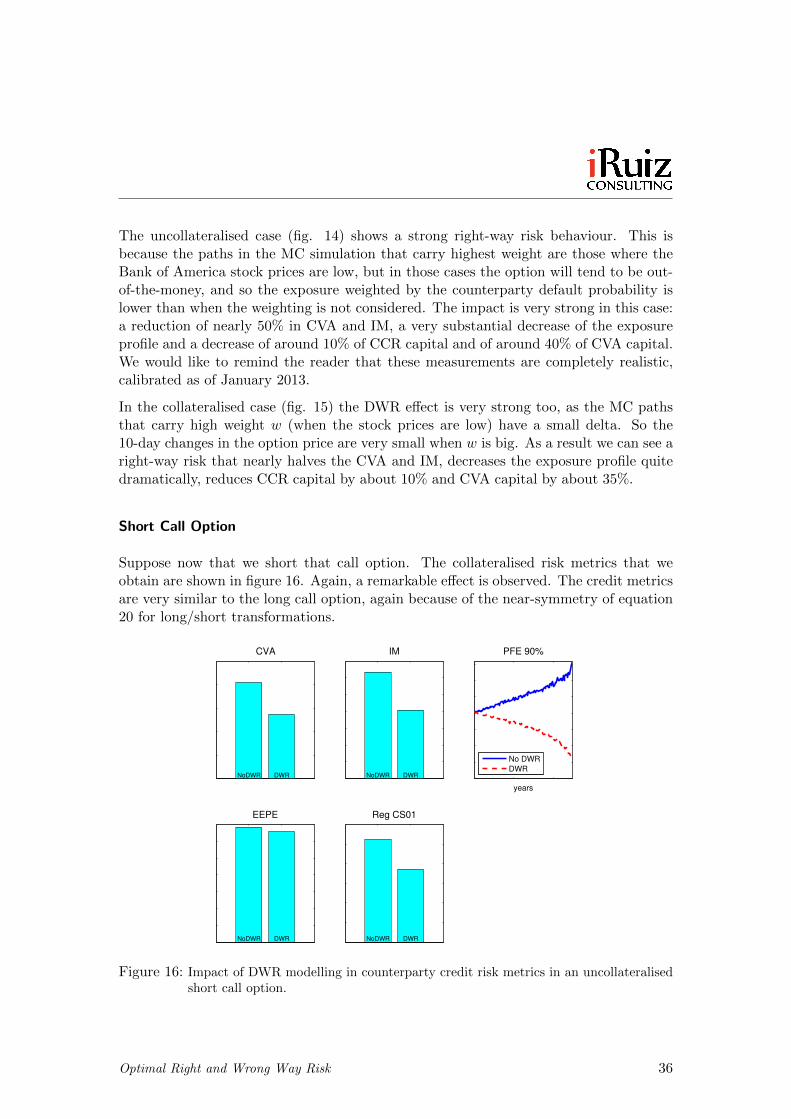
The uncollateralised case (fig. 14) shows a strong right-way risk behaviour. This isbecause the paths in the MC simulation that carry highest weight are those where theBank of America stock prices are low, but in those cases the option will tend to be out-of-the-money, and so the exposure weighted by the counterparty default probability islower than when the weighting is not considered. The impact is very strong in this case:a reduction of nearly 50% in CVA and IM, a very substantial decrease of the exposureprofile and a decrease of around 10% of CCR capital and of around 40% of CVA capital.We would like to remind the reader that these measurements are completely realistic,calibrated as of January 2013.
In the collateralised case (fig. 15) the DWR effect is very strong too, as the MC pathsthat carry high weight w (when the stock prices are low) have a small delta. So the10-day changes in the option price are very small when w is big. As a result we can see aright-way risk that nearly halves the CVA and IM, decreases the exposure profile quitedramatically, reduces CCR capital by about 10% and CVA capital by about 35%.
Short Call Option
Suppose now that we short that call option. The collateralised risk metrics that weobtain are shown in figure 16. Again, a remarkable effect is observed. The credit metricsare very similar to the long call option, again because of the near-symmetry of equation20 for long/short transformations.
CVA
NoDWR DWR
IM
NoDWR DWR
years
PFE 90%
No DWR
DWR
EEPE
NoDWR DWR
Reg CS01
NoDWR DWR
Figure 16: Impact of DWR modelling in counterparty credit risk metrics in an uncollateralisedshort call option.
Optimal Right and Wrong Way Risk 36
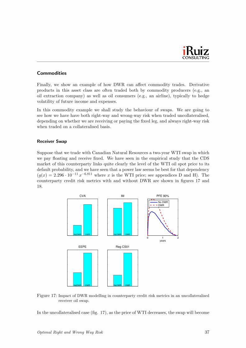
Commodities
Finally, we show an example of how DWR can affect commodity trades. Derivativeproducts in this asset class are often traded both by commodity producers (e.g., anoil extraction company) as well as oil consumers (e.g., an airline), typically to hedgevolatility of future income and expenses.
In this commodity example we shall study the behaviour of swaps. We are going tosee how we have have both right-way and wrong-way risk when traded uncollateralised,depending on whether we are receiving or paying the fixed leg, and always right-way riskwhen traded on a collateralised basis.
Receiver Swap
Suppose that we trade with Canadian Natural Resources a two-year WTI swap in whichwe pay floating and receive fixed. We have seen in the empirical study that the CDSmarket of this counterparty links quite clearly the level of the WTI oil spot price to itsdefault probability, and we have seen that a power law seems be best for that dependency(g(x) = 2.296 · 10−11 x−6.811 where x is the WTI price; see appendices D and H). Thecounterparty credit risk metrics with and without DWR are shown in figures 17 and18.
CVA
NoDWR DWR
IM
NoDWR DWR
0 1 2years
PFE 90%
EEPE
NoDWR DWR
Reg CS01
NoDWR DWR
No DWR
DWR
Figure 17: Impact of DWR modelling in counterparty credit risk metrics in an uncollateralisedreceiver oil swap.
In the uncollateralised case (fig. 17), as the price of WTI decreases, the swap will become
Optimal Right and Wrong Way Risk 37
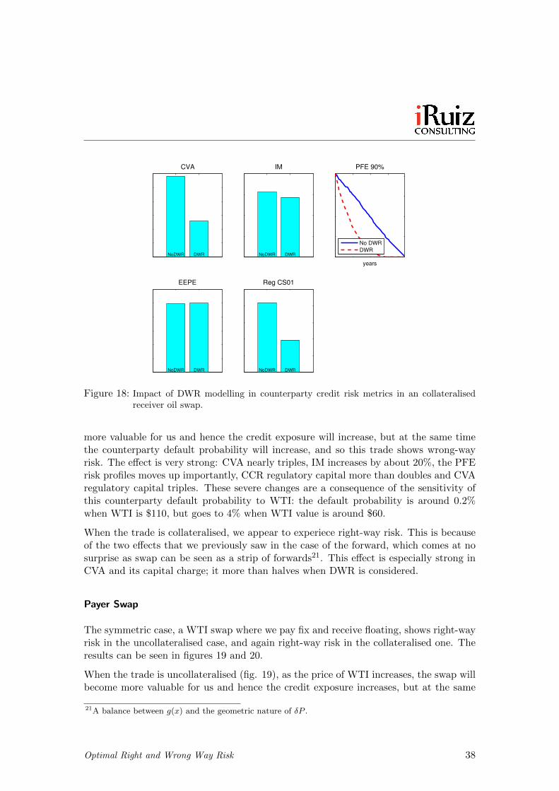
CVA
NoDWR DWR
IM
NoDWR DWR
years
PFE 90%
EEPE
NoDWR DWR
Reg CS01
NoDWR DWR
No DWR
DWR
Figure 18: Impact of DWR modelling in counterparty credit risk metrics in an collateralisedreceiver oil swap.
more valuable for us and hence the credit exposure will increase, but at the same timethe counterparty default probability will increase, and so this trade shows wrong-wayrisk. The effect is very strong: CVA nearly triples, IM increases by about 20%, the PFErisk profiles moves up importantly, CCR regulatory capital more than doubles and CVAregulatory capital triples. These severe changes are a consequence of the sensitivity ofthis counterparty default probability to WTI: the default probability is around 0.2%when WTI is $110, but goes to 4% when WTI value is around $60.
When the trade is collateralised, we appear to experiece right-way risk. This is becauseof the two effects that we previously saw in the case of the forward, which comes at nosurprise as swap can be seen as a strip of forwards21. This effect is especially strong inCVA and its capital charge; it more than halves when DWR is considered.
Payer Swap
The symmetric case, a WTI swap where we pay fix and receive floating, shows right-wayrisk in the uncollateralised case, and again right-way risk in the collateralised one. Theresults can be seen in figures 19 and 20.
When the trade is uncollateralised (fig. 19), as the price of WTI increases, the swap willbecome more valuable for us and hence the credit exposure increases, but at the same
21A balance between g(x) and the geometric nature of δP .
Optimal Right and Wrong Way Risk 38
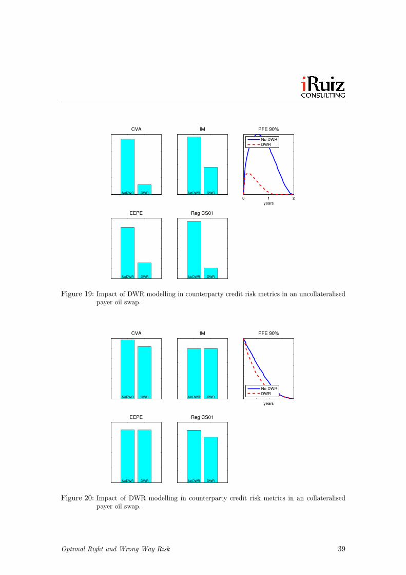
CVA
NoDWR DWR
IM
NoDWR DWR
0 1 2years
PFE 90%
EEPE
NoDWR DWR
Reg CS01
NoDWR DWR
No DWR
DWR
Figure 19: Impact of DWR modelling in counterparty credit risk metrics in an uncollateralisedpayer oil swap.
CVA
NoDWR DWR
IM
NoDWR DWR
years
PFE 90%
EEPE
NoDWR DWR
Reg CS01
NoDWR DWR
No DWR
DWR
Figure 20: Impact of DWR modelling in counterparty credit risk metrics in an collateralisedpayer oil swap.
Optimal Right and Wrong Way Risk 39

time the counterparty default probability will decrease, and hence this trades showsright-way risk. This effect is again dramatic as a result of the strength of the market-credit dependency captured by g(x): CVA gets divided by around 6, IM more thanhalves, the exposure profile is strongly reduced and both CCR and CVA capital alsodecrease most heavily.
In the collateralised case we have a similar effect as described in the receiver swap, asexpected22. This effect seems to be smoother this time, though.
A Remark on this Example
We would like to draw the reader’s attention to this example, as in the authors’ viewsit demonstrates the strength of the DWR model used.
We are calibrating the Empirical Analysis approach to model DWR to real data as ofJanuary 2013. As a result we are easily able to incorporate into our DWR model the em-pirically measured dependency structure between the credit quality of the counterpartyand the market factors, as opposed to a “guesstimate” of it, which is the best you canaim for in all other modelling frameworks. As a consequence, we are actually matchingthe intensity of the DWR effect to that indicated by the market. In this example weobserve a very significant reduction in several credit risk metrics when DWR effects areconsidered. Such reduction would, in our experience working for many years in financialinstituions, be very difficult to justify to a regulator, for example, without a data-drivenmodelling framework like this one. Also, it reduces model risk as it removes subjectivejudgement by the research team.
Sensitivities
So far we have seen how the main counterparty credit risk metrics (CVA, Initial Margin,PFE exposure and Regulatory Capital) can vary notably in options, forwards and swapswhen considering DRW effects. We have reviewed examples where the source of DWRcomes from the equity, FX and commodity markets. In addition to this, the sensitivitiesof these metrics can also be importantly affected by DWR.
We have seen already some of this by studying the impact of the DWR model in theregulatory CVA-CS01. To illustrate this case further, we make use of the payer WTIswap from before, and observe how the CVA changes as the WTI volatility varies. Weillustrate this here by plotting the CVA price and the CVA vega for different values ofthe WTI volatility, all else remaining constant. The results are shown in figure 21, bothin an uncollateralised and collateralised basis.
The effect is quite remarkable in both cases. In the uncollateralised case, DWR effectschange the Vega most strongly; in fact its sign even changes. In the collateralised case
22As being long a receiver swap is being short a payer swap
Optimal Right and Wrong Way Risk 40
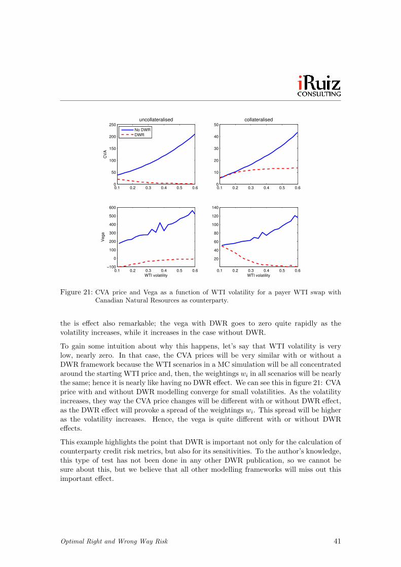
0.1 0.2 0.3 0.4 0.5 0.60
50
100
150
200
250
CV
A
uncollateralised
0.1 0.2 0.3 0.4 0.5 0.60
10
20
30
40
50
collateralised
0.1 0.2 0.3 0.4 0.5 0.6−100
0
100
200
300
400
500
600
WTI volatility
Vega
0.1 0.2 0.3 0.4 0.5 0.6
20
40
60
80
100
120
140
WTI volatility
No DWR
DWR
Figure 21: CVA price and Vega as a function of WTI volatility for a payer WTI swap withCanadian Natural Resources as counterparty.
the is effect also remarkable; the vega with DWR goes to zero quite rapidly as thevolatility increases, while it increases in the case without DWR.
To gain some intuition about why this happens, let’s say that WTI volatility is verylow, nearly zero. In that case, the CVA prices will be very similar with or without aDWR framework because the WTI scenarios in a MC simulation will be all concentratedaround the starting WTI price and, then, the weightings wi in all scenarios will be nearlythe same; hence it is nearly like having no DWR effect. We can see this in figure 21: CVAprice with and without DWR modelling converge for small volatilities. As the volatilityincreases, they way the CVA price changes will be different with or without DWR effect,as the DWR effect will provoke a spread of the weightings wi. This spread will be higheras the volatility increases. Hence, the vega is quite different with or without DWReffects.
This example highlights the point that DWR is important not only for the calculation ofcounterparty credit risk metrics, but also for its sensitivities. To the author’s knowledge,this type of test has not been done in any other DWR publication, so we cannot besure about this, but we believe that all other modelling frameworks will miss out thisimportant effect.
Optimal Right and Wrong Way Risk 41
A Few Practical Points
We have seen that the impact of DWR in counterparty credit risk metrics can be im-portant. We have studied cases in which the source of the DWR lies in the equity, FXand commodity markets.
The choice of the market factor It must be noted that, for some counterparties, twoor three of these models may be applicable. For example, in the case of a major oilcompany in an emerging economy, we may be able to use as the DWR driving asseteither its equity price, an FX rate or a commodity price. Which to use best will dependin the nature of those dependencies and may also be driven by practical considerationslike the models and infrastructure that a financial institution already has in place.
In some other cases only one of the models may be applicable; for example, if thecounterparty is a small oil company, whose balance sheet is not very sensitive to swingsin the FX market, and without a traded equity. In this case, it is sensible to use the oilprice as the DWR driving asset.
Calibration We have seen that the Empirical Analysis approach for modelling DWR isoptimal from a calibration standpoint compared to the other ones. However, this doesnot mean that calibration will always be a trivial exercise. This is because data canbe limited; for example, in the previous case of a small oil company, we may have toestimate its g(x) using a variety of techniques, which may include benchmarking its g(x)function to other similar companies for which data exists. However, in any case, thismethodology maximises the utilisation of the available data when it is limited, which is,in our view, one of its key strengths.
Implementation effort Finally, it should be noted that the examples have showed theeffect of DWR in single trades. In practice, most often we will have a portfolio of trades(as opposed to a single trade) with a given counteparty in the same netting set. In thatcase we will have to chose the best DWR driving asset in the same way as we have donefor one trade, and then we need a dependency structure between that asset “x” and allother risk factors that drive the valuation of the portfolio.
Outcome of this section
In this section we have observed, using a number of realistic examples, the followingpoints.
1. The CVA, initial margin, exposure profiles and capital calculation can change quitedramatically when DWR is considered.
Optimal Right and Wrong Way Risk 42
2. This change can be important in either the right-way or wrong-way risk direction,so both must be considered.
3. When uncollateralised, it is the case that when one trade shows wrong-way risk,its opposite trade (i.e. long or short) shows right-way risk.
4. When a trade is in a collateral agreement, its DWR behaviour can be very differentto the uncollateralised case. In fact, its behaviour is more complex and difficult toanticipate, as it is driven by in a balance between the (i) the trade delta distributionacross the values of x (∆(x)), (ii) the strength of the DWR effect given by thefunction g(x) and (iii) diffusion nature of the risk factors (e.g. normal V. log-normal). We have also seen that, when collateralised, trades show similar DWRbehaviour whether we are long or short23.
Conclusions
We are now in a position to answer the questions raised at the beginning of this pa-per.
What is the optimal way to model DWR? In the authors’ opinion, the EmpiricalAnalysis methodology is optimal for modelling DWR24. This is because it is the onlyone that achieve all the following goals.
1. It has a robust modelling framework, and it uses the observed market-credit de-pendency structure, as opposed to a guess of how that dependency structure couldbe.
2. It can be directly and easily calibrated to data.
3. Its implementation requires minimal work, as it makes uses of existing Monte Carlosimulations without DWR.
4. Its impact in the every-day work of a financial institution can be high, as it isbased on an intuitive methodology that is data-driven, and it does not make useof latent non-observable abstract variables.
What is the actual extent of DWR in a financial institution? We have seen froma number of real examples that DWR can be highly relevant. Our realistic examplescalibrated as of January 2013 show that CVA, initial margin, exposure profiles and cap-ital can change significantly; indeed, we have observed a case in which CVA decreased
23In the context of the ideal CSA used in the example of this study.24Perhaps with the special exception of collateralised FX trades with emerging markets sovereign, where
the default itself can trigger a jump in the underlying market and, hence, a scenario-based approachmay be needed as explained.
Optimal Right and Wrong Way Risk 43
around six times. Those tests had to be done with single trades as each financial institu-tion will have a different book of trades and, hence, it will be difficult to obtain resultsthat can be applicable to all institutions, but those tests show that DWR can be quiteimportant, and that it must be dealt with carefully.
What happens if this DWR is not properly modelled? The data analysed suggeststhat the market-credit dependency structure that provokes DWR can be modelled bylinking the default probabilities to levels of a market risk factor. We have also seen thatthe correlation in the changes between those factors and credit drivers is not constant,but in fact depends on the level of the market factor. In our view, a good model forDWR should reflect this.
We have also seen how DWR can change the credit exposure metrics of a book of tradesnoticeably, both for collateralised and uncollateralised facilities. Moreover, the driversof DWR effects are very different in each of those cases. If uncollateralised, the directionof the DWR effect tends to get inverted when we change the long/short direction. Ifcollateralised, a long/short transformation tends to keep the same DWR effect.
If a good DWR model is not considered, the counterparty credit risk calculation andrisk allocation within an organisation will not adequately reflect the true economic risksthat the institution is carrying. As a result, management will not be aware of someactual risks, and it will be bound to make wrong decisions, while incentives will be inap-propiately allocated in the organisation and the institution will be exposed to negativeevents, that are not known to the organisation, and that could have been anticipatedand managed pre-emptively with a good DWR model.
A good DWR model will not only reverse those problems, but could also allow a bankto decrease its regulatory capital. This is because, firstly, it may apply to its regulatorsfor a reduction in its α multiplier for capital calculation and, secondly, the EEPE andregulatory CVA-CS01 that drive the capital calculation will be reduced in those nettingsets that carry right-way risk. Regulators should be open to these changes as, on thisway, they will create the incentives for banks to manage DWR properly. Within thecurrent Basel framework and regulatory policy, risk assessment and allocation is notcorrect, and incentives to improve the risk management set up regarding DWR are quitenon-existent. The author’s believe this is an important mistake.
Do we need to consider both right-way and wrong-way risk? We should indeedconsider both these factors. Currenlty, DWR is mainly focused in wrong-way risk in theindustry; the term “right-way risk” is hardly ever mentioned, while “wrong-way risk”very often. However, this study shows that right-way is as important as wrong-way forthe proper understanding of the economic risks that an institution carries, and so bothought to be considered in parallel.
Optimal Right and Wrong Way Risk 44

Acknowledgements
The authors would like to thank Jonathan Campbell, Ersel Korusoy and Christian Morrisfor interesting feedback on an early version of this paper.
Optimal Right and Wrong Way Risk 45
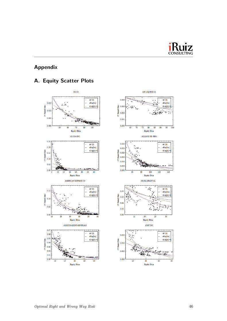
Appendix
A. Equity Scatter Plots
Optimal Right and Wrong Way Risk 46
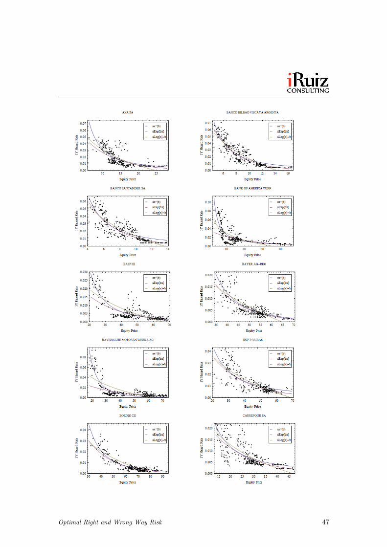
Optimal Right and Wrong Way Risk 47
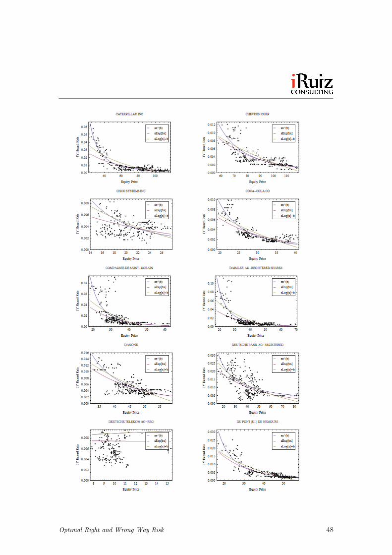
Optimal Right and Wrong Way Risk 48
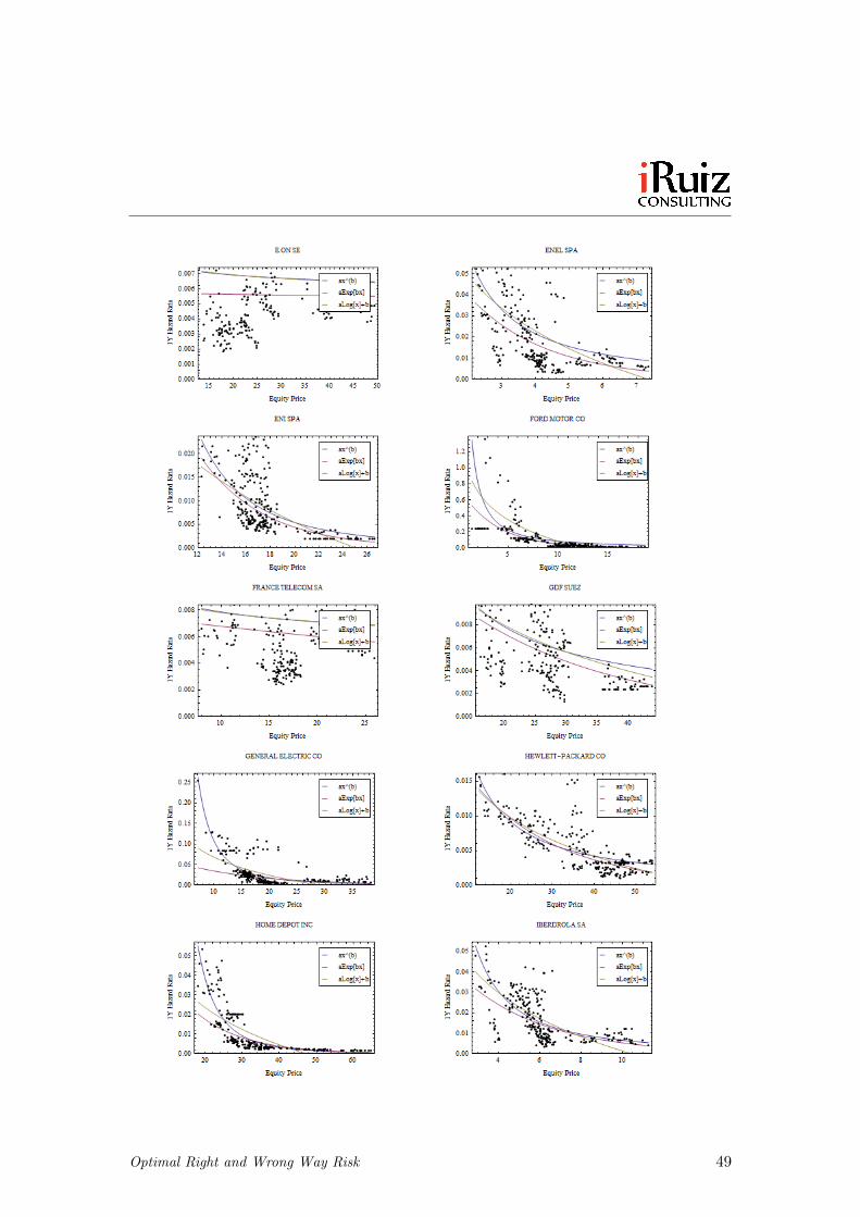
Optimal Right and Wrong Way Risk 49
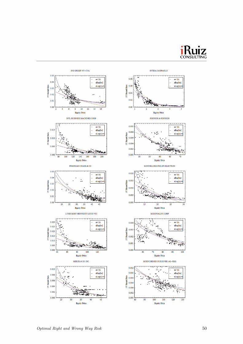
Optimal Right and Wrong Way Risk 50
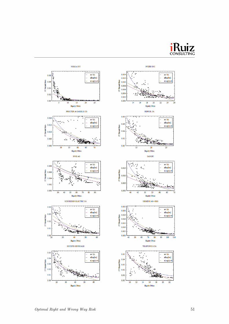
Optimal Right and Wrong Way Risk 51
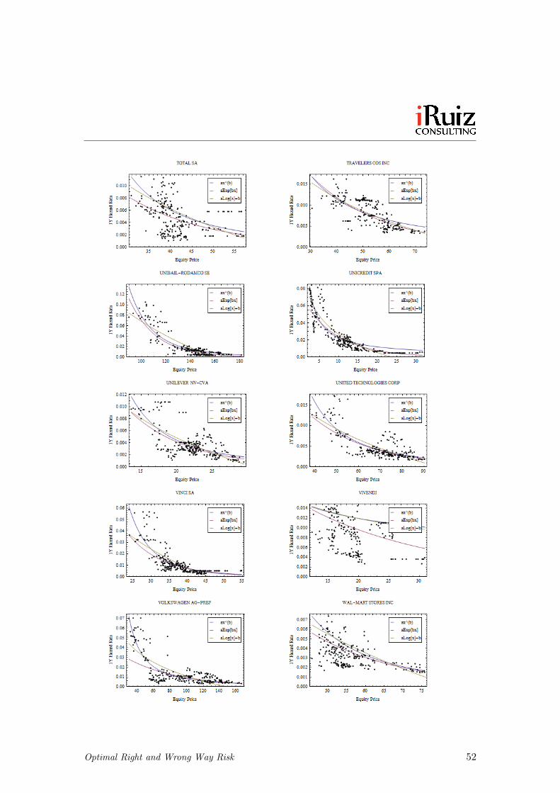
Optimal Right and Wrong Way Risk 52
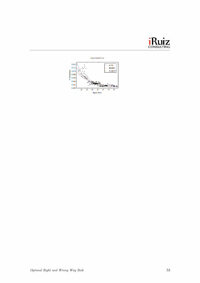
Optimal Right and Wrong Way Risk 53

B. Government FX Scatter Plots
Optimal Right and Wrong Way Risk 54
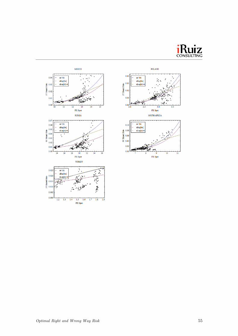
Optimal Right and Wrong Way Risk 55
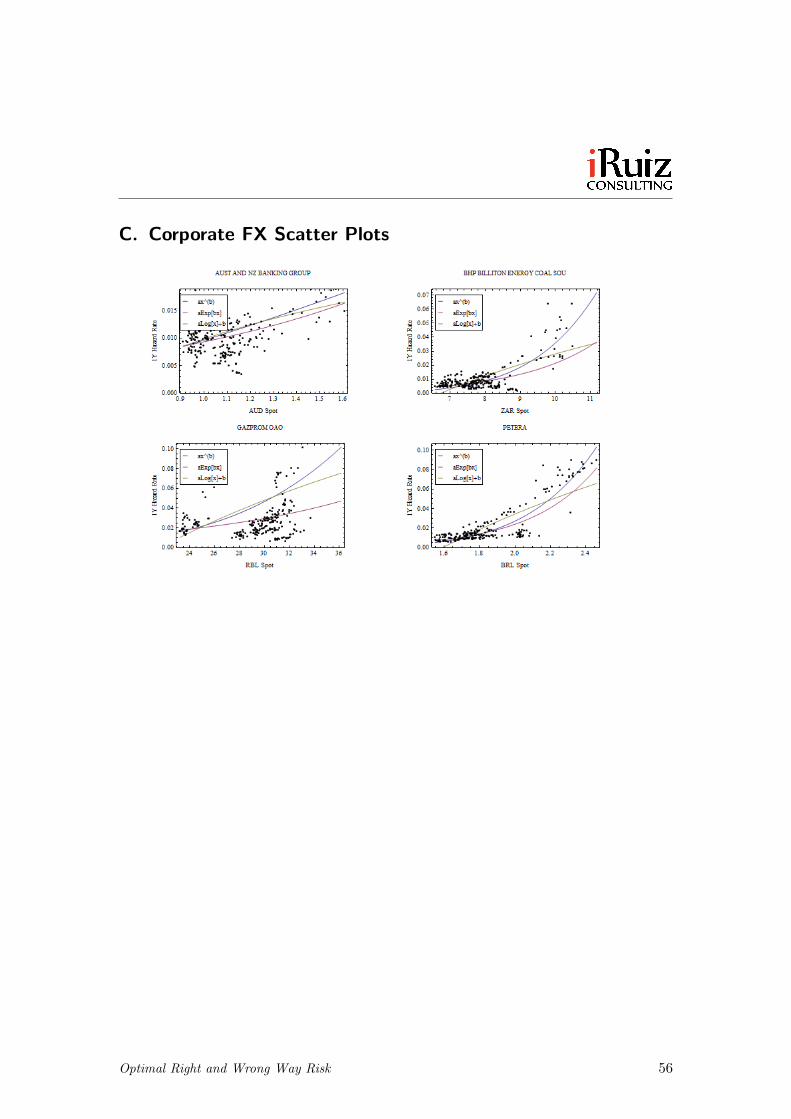
C. Corporate FX Scatter Plots
Optimal Right and Wrong Way Risk 56

D. Commodity Scatter Plots
Optimal Right and Wrong Way Risk 57
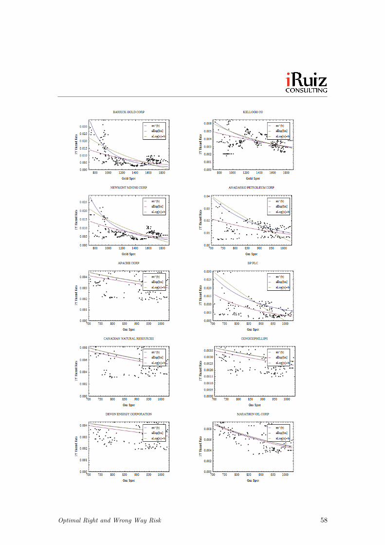
Optimal Right and Wrong Way Risk 58
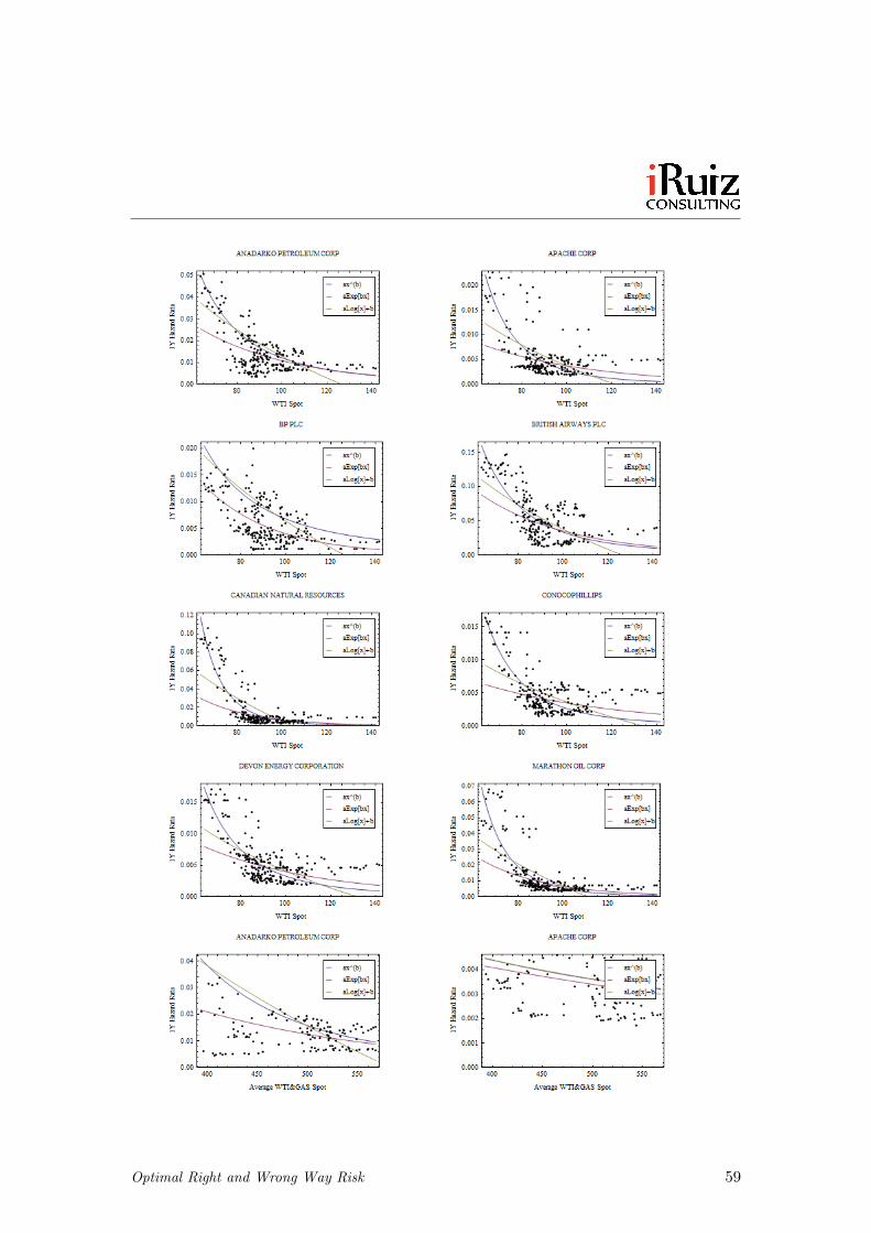
Optimal Right and Wrong Way Risk 59
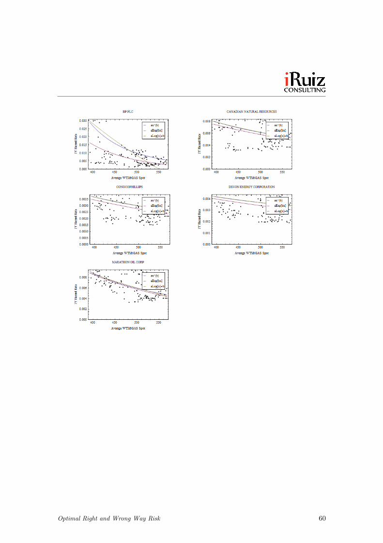
Optimal Right and Wrong Way Risk 60
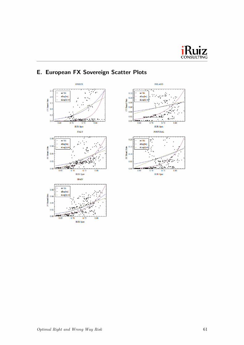
E. European FX Sovereign Scatter Plots
Optimal Right and Wrong Way Risk 61
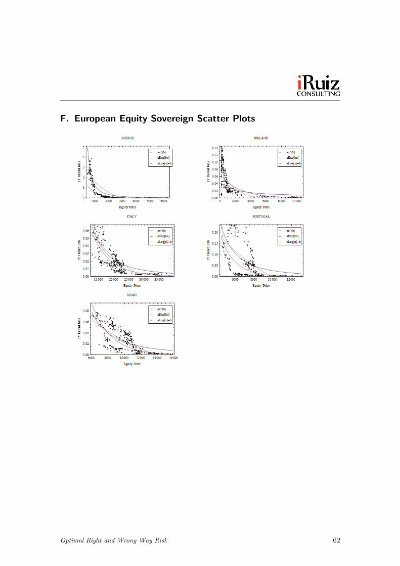
F. European Equity Sovereign Scatter Plots
Optimal Right and Wrong Way Risk 62
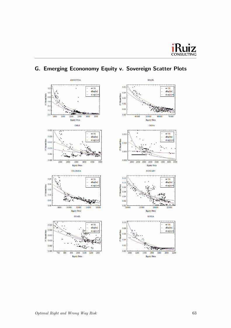
G. Emerging Econonomy Equity v. Sovereign Scatter Plots
Optimal Right and Wrong Way Risk 63
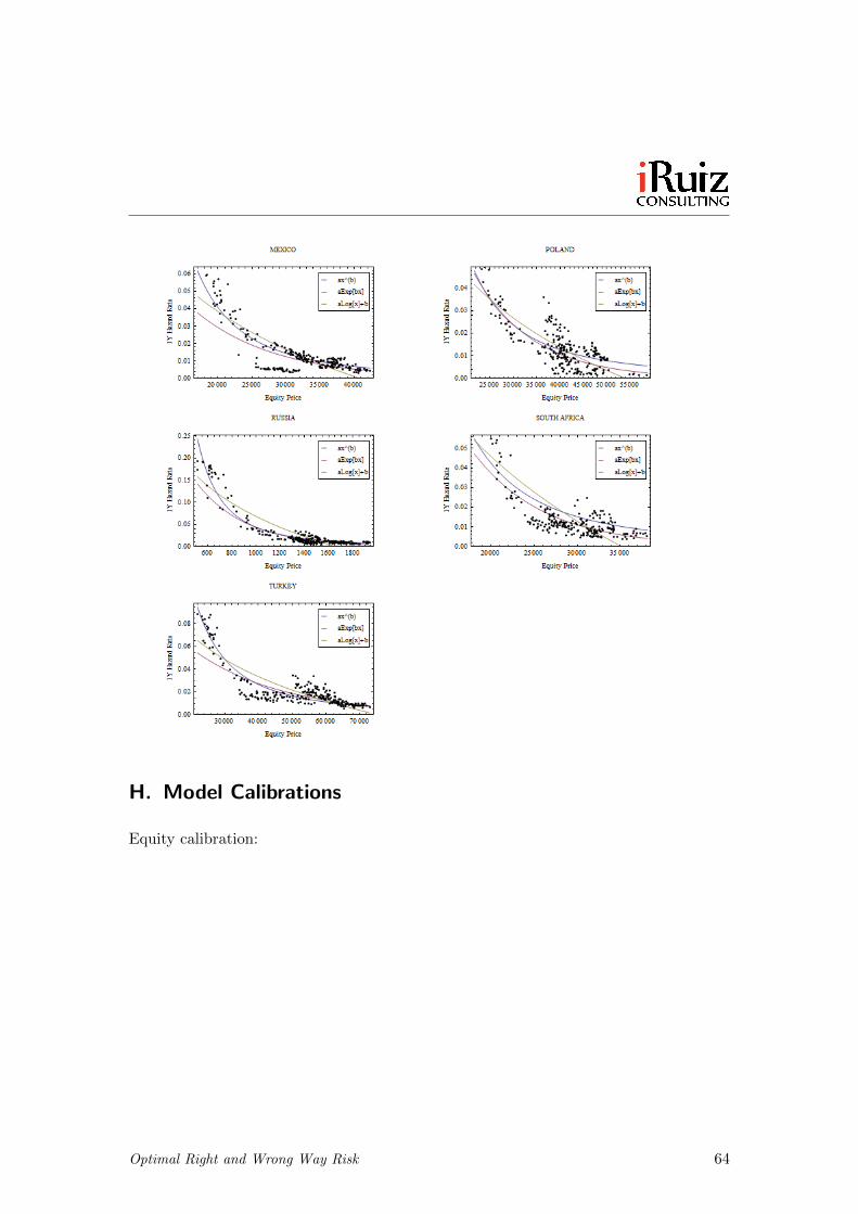
H. Model Calibrations
Equity calibration:
Optimal Right and Wrong Way Risk 64
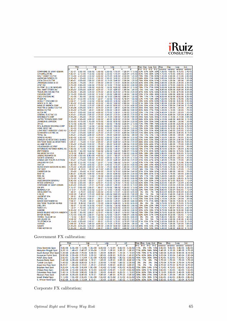
Government FX calibration:
Corporate FX calibration:
Optimal Right and Wrong Way Risk 65
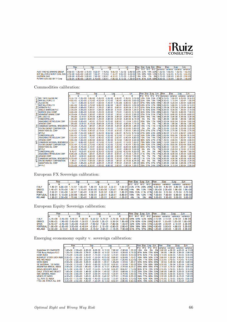
Commodities calibration:
European FX Sovereign calibration:
European Equity Sovereign calibration:
Emerging economomy equity v. sovereign calibration:
Optimal Right and Wrong Way Risk 66
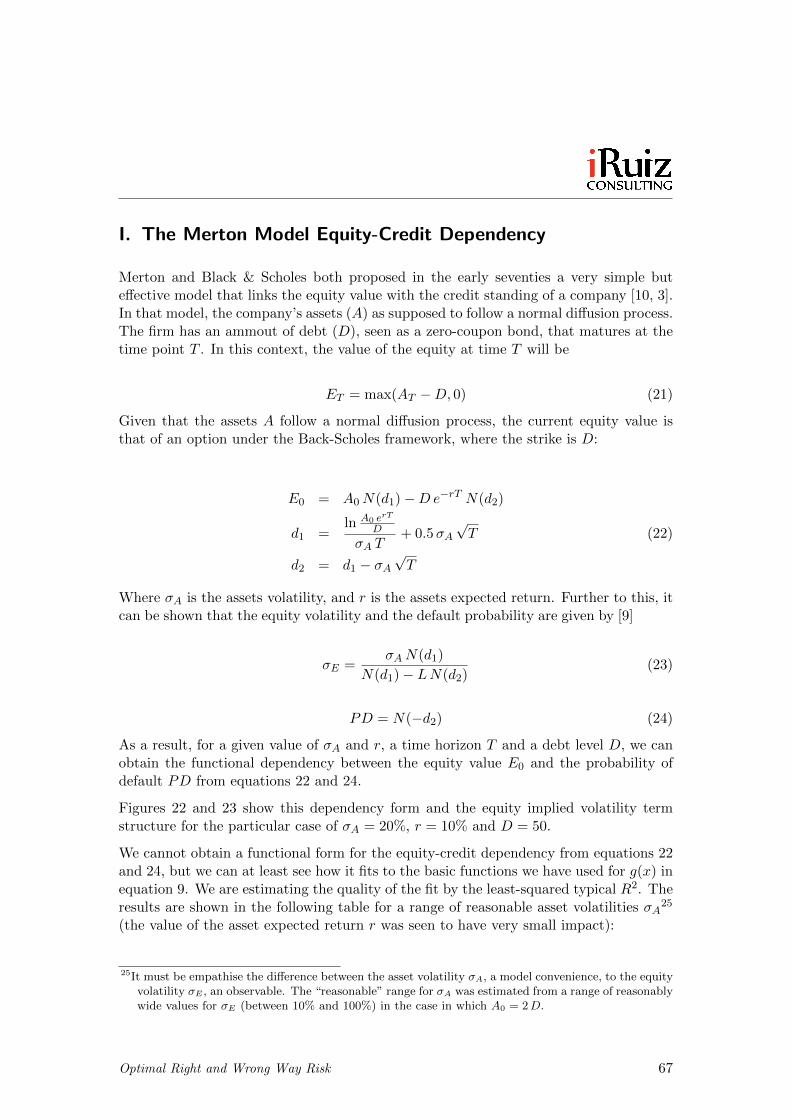
I. The Merton Model Equity-Credit Dependency
Merton and Black & Scholes both proposed in the early seventies a very simple buteffective model that links the equity value with the credit standing of a company [10, 3].In that model, the company’s assets (A) as supposed to follow a normal diffusion process.The firm has an ammout of debt (D), seen as a zero-coupon bond, that matures at thetime point T . In this context, the value of the equity at time T will be
ET = max(AT −D, 0) (21)
Given that the assets A follow a normal diffusion process, the current equity value isthat of an option under the Back-Scholes framework, where the strike is D:
E0 = A0N(d1)−De−rT N(d2)
d1 =ln A0 erT
D
σA T+ 0.5σA
√T (22)
d2 = d1 − σA√T
Where σA is the assets volatility, and r is the assets expected return. Further to this, itcan be shown that the equity volatility and the default probability are given by [9]
σE =σAN(d1)
N(d1)− LN(d2)(23)
PD = N(−d2) (24)
As a result, for a given value of σA and r, a time horizon T and a debt level D, we canobtain the functional dependency between the equity value E0 and the probability ofdefault PD from equations 22 and 24.
Figures 22 and 23 show this dependency form and the equity implied volatility termstructure for the particular case of σA = 20%, r = 10% and D = 50.
We cannot obtain a functional form for the equity-credit dependency from equations 22and 24, but we can at least see how it fits to the basic functions we have used for g(x) inequation 9. We are estimating the quality of the fit by the least-squared typical R2. Theresults are shown in the following table for a range of reasonable asset volatilities σA
25
(the value of the asset expected return r was seen to have very small impact):
25It must be empathise the difference between the asset volatility σA, a model convenience, to the equityvolatility σE , an observable. The “reasonable” range for σA was estimated from a range of reasonablywide values for σE (between 10% and 100%) in the case in which A0 = 2D.
Optimal Right and Wrong Way Risk 67
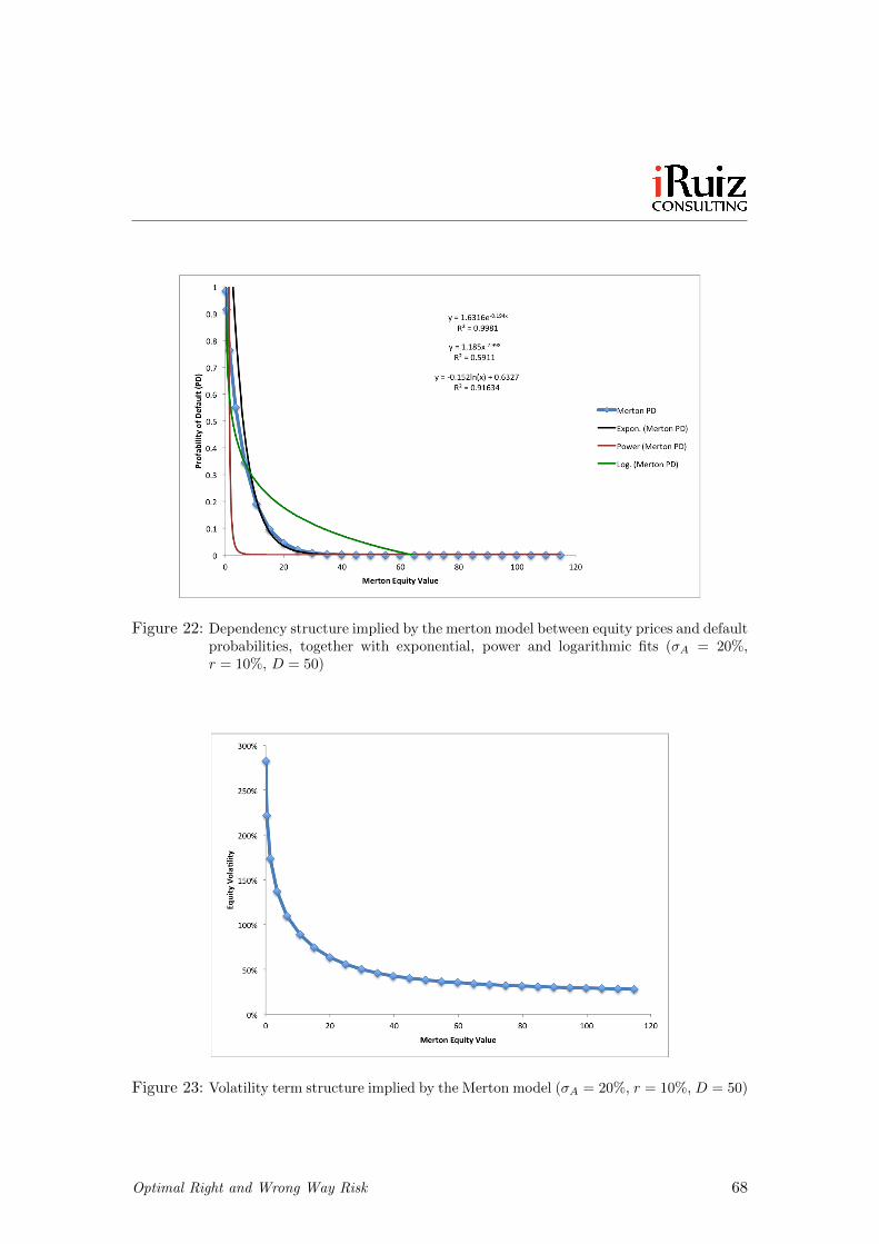
Figure 22: Dependency structure implied by the merton model between equity prices and defaultprobabilities, together with exponential, power and logarithmic fits (σA = 20%,r = 10%, D = 50)
Figure 23: Volatility term structure implied by the Merton model (σA = 20%, r = 10%, D = 50)
Optimal Right and Wrong Way Risk 68
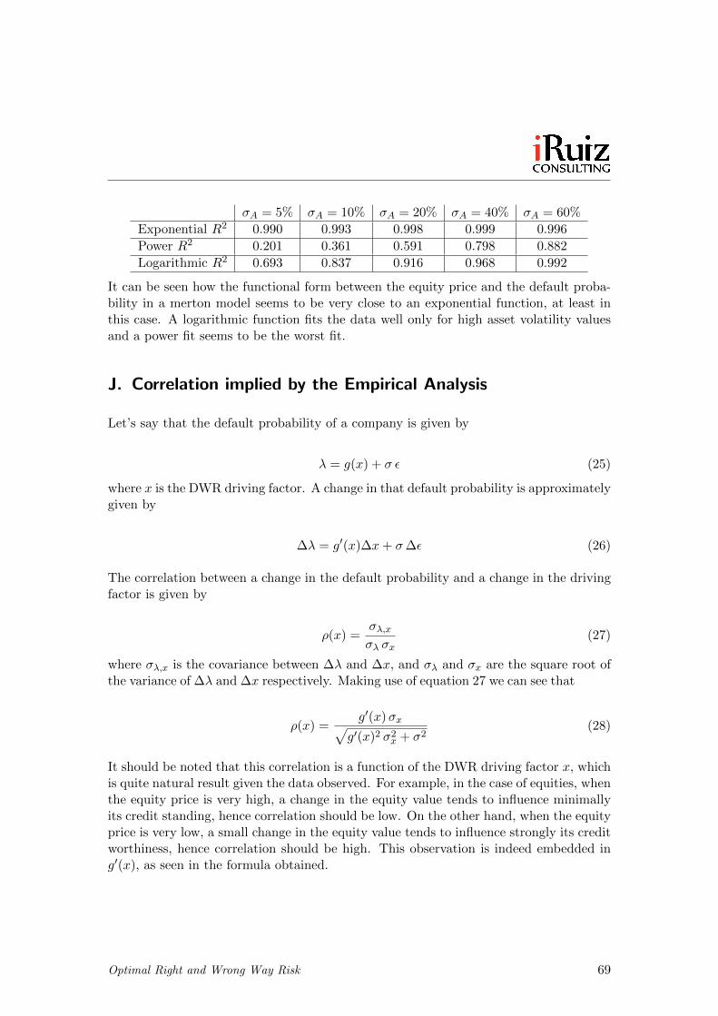
σA = 5% σA = 10% σA = 20% σA = 40% σA = 60%
Exponential R2 0.990 0.993 0.998 0.999 0.996
Power R2 0.201 0.361 0.591 0.798 0.882
Logarithmic R2 0.693 0.837 0.916 0.968 0.992
It can be seen how the functional form between the equity price and the default proba-bility in a merton model seems to be very close to an exponential function, at least inthis case. A logarithmic function fits the data well only for high asset volatility valuesand a power fit seems to be the worst fit.
J. Correlation implied by the Empirical Analysis
Let’s say that the default probability of a company is given by
λ = g(x) + σ ε (25)
where x is the DWR driving factor. A change in that default probability is approximatelygiven by
∆λ = g′(x)∆x+ σ∆ε (26)
The correlation between a change in the default probability and a change in the drivingfactor is given by
ρ(x) =σλ,xσλ σx
(27)
where σλ,x is the covariance between ∆λ and ∆x, and σλ and σx are the square root ofthe variance of ∆λ and ∆x respectively. Making use of equation 27 we can see that
ρ(x) =g′(x)σx√
g′(x)2 σ2x + σ2(28)
It should be noted that this correlation is a function of the DWR driving factor x, whichis quite natural result given the data observed. For example, in the case of equities, whenthe equity price is very high, a change in the equity value tends to influence minimallyits credit standing, hence correlation should be low. On the other hand, when the equityprice is very low, a small change in the equity value tends to influence strongly its creditworthiness, hence correlation should be high. This observation is indeed embedded ing′(x), as seen in the formula obtained.
Optimal Right and Wrong Way Risk 69
References
[1] International convergence of capital measurement and capital standards, tech. rep., Bankfor International Settlements, 2006.
[2] Revision to the basel ii market risk framework, tech. rep., Bank for International Settlements,2009.
[3] F. Black and M. Scholes, The pricing of options and corporate liabilities, Journal ofPolitical Economy, (1973).
[4] G. Cesari, J. Aquilina, N. Carpillon, Z. Filipovic, G. Lee, and I. Manda, Mod-elling, Pricing and Hedging Counterparty Credit Exposure, Springer, first ed., 2009.
[5] J. C. G. Cespedes, J. A. de Juan Herrero, D. Rosen, and D. Sounders, Effectivemodeling of wrong way risk, counterparty credit risk capital, and alpha in basel ii, TheJournal of Risk Model Validation, 4 (2010), pp. 71–98.
[6] P.-E. Chabanel, Basel iii. Moody’s Analytics, May 2011.
[7] J. Hull and A. White, Cva and wrong way risk, Financial Analysis Journal, 68 (2012),pp. 58–69.
[8] F. Iacono, Quantifying right-way and wrong-way risk, Riverside Risk Advisors, 1 (2011).
[9] E. P. Jones, S. P. Mason, and E. Rosenfeld, Contingent claims analysis of corportecapital structure: An empirical investigation, Journal of Finance, 39 (1984).
[10] R. C. Merton, On the pricing of corporate debt: The risk structure of interest rates,Journal of Finance, 3 (1974).
[11] B. C. of Banking Supervision, Bassel iii: A global regulatory framework for more re-silient banks and banking system, tech. rep., Bank for International Settlements, 2011.
[12] D. Rosen and D. Saunders, Cva the wrong way, Journal of Risk Management in FinancialInstitutions, 5 (2012), pp. 152–272.
[13] I. Ruiz, Technical note: On wrong way risk. www.iruizconsulting.com, February 2012.
[14] M. Turlakov, Wrong-way risk, credit and funding, Risk Magazine, 1 (2013).
Optimal Right and Wrong Way Risk 70