DI

SC

US

SI

ON

P

AP

ER

S

ER

IE

S

Forschungsinstitut zur Zukunft der ArbeitInstitute for the Study of Labor

Optimal Piecewise Linear Income Taxation

IZA DP No. 6007

October 2011

Patricia AppsNgo Van LongRay Rees

Optimal Piecewise Linear Income Taxation

Patricia Apps University of Sydney

and IZA

Ngo Van Long McGill University

Ray Rees

University of Munich and CES

Discussion Paper No. 6007 October 2011

IZA

P.O. Box 7240 53072 Bonn

Germany

Phone: +49-228-3894-0 Fax: +49-228-3894-180

E-mail: iza@iza.org

Any opinions expressed here are those of the author(s) and not those of IZA. Research published in this series may include views on policy, but the institute itself takes no institutional policy positions. The Institute for the Study of Labor (IZA) in Bonn is a local and virtual international research center and a place of communication between science, politics and business. IZA is an independent nonprofit organization supported by Deutsche Post Foundation. The center is associated with the University of Bonn and offers a stimulating research environment through its international network, workshops and conferences, data service, project support, research visits and doctoral program. IZA engages in (i) original and internationally competitive research in all fields of labor economics, (ii) development of policy concepts, and (iii) dissemination of research results and concepts to the interested public. IZA Discussion Papers often represent preliminary work and are circulated to encourage discussion. Citation of such a paper should account for its provisional character. A revised version may be available directly from the author.

IZA Discussion Paper No. 6007 October 2011

ABSTRACT

Optimal Piecewise Linear Income Taxation*

Given its significance in practice, piecewise linear taxation has received relatively little attention in the literature. This paper offers a simple and transparent analysis of its main characteristics. We fully characterize optimal tax parameters for the cases in which budget sets are convex and nonconvex respectively. A numerical analysis of a discrete version of the model shows the circumstances under which each of these cases will hold as a global optimum. We find that, given plausible parameter values and wage distributions, the globally optimal tax system is convex, and marginal rate progressivity increases with rising inequality. JEL Classification: H21, H31, J22 Keywords: piecewise linear, income, taxation Corresponding author: Patricia Apps Faculty of Law University of Sydney Eastern Avenue, Camperdown Campus Sydney NSW 2006 Australia E-mail: patricia.apps@sydney.edu.au

* We would like to thank Michael Hoy, Efraim Sadka and two referees, as well as seminar participants at IZA and Vanderbilt University, for very helpful comments. We are also grateful to Yuri Andrienko and Piers Trepper for research assistance. The usual disclaimer applies. This research was supported under the Australian Research Council’s DP Funding Scheme (DP 0881787).

1 Introduction

The foundations of the theory of optimal income taxation were provided bythe theory of nonlinear taxation �rst developed by James Mirrlees (1971),and the theory of linear taxation formulated by Eytan Sheshinski (1972).In Mirrlees�s analysis, the problem is seen as one of mechanism design. Anoptimally chosen menu of marginal tax rates and lump sum tax/subsidiesis o¤ered, and individuals select from this menu in a way that reveals theirproductivity type. As well as the government budget constraint therefore, akey role is played by incentive compatibility or self selection constraints.In Sheshinski�s linear tax analysis on the other hand, there is no attempt

to solve the mechanism design problem. All individuals are pooled, and theproblem is to �nd the optimal marginal tax rate and lump sum payment overthe working population as a whole, subject only to the government budgetconstraint.In each case, the theory provides an analysis of how concerns with the

equity and e¢ ciency of a tax system interact to determine the parametersof that system, and in particular its marginal rate structure and degree ofprogressivity.As Boadway (1998) points out, the optimal nonlinear tax is Pareto supe-

rior to a linear tax for any given revenue requirement and set of consumers,implying a superior tradeo¤ between equity and e¢ ciency. Nevertheless,tax policy makers or "central planners" do not seem to adopt the Mirrleesapproach to the design of tax systems in practice.In reality virtually all tax systems are neither linear in the sense of

Sheshinski nor nonlinear in the sense of Mirrlees, but rather piecewise linear.Gross income is divided into (usually relatively few) brackets and marginaltax rates are constant within but vary across these brackets.1 When we con-sider formal income tax systems, the marginal tax rates are typically strictlyincreasing with the income levels de�ning the brackets. We refer to thiscase of strict marginal rate progressivity as the convex case, since it de�nesfor an income earner a convex budget set in the space of gross income-netincome/consumption. However, when we widen the de�nition of the tax sys-tem to include cash transfers that are paid and withdrawn as a function of

1The German tax system is a rare exception to this. It has four brackets and in thesecond and third of these marginal tax rates increase linearly with income. However, this islikely to be replaced by a more conventional step function in future. For further discussionsee Apps and Rees (2009).

2

gross income we see that typically this may lead marginal tax rates to fallover some range as gross income increases. Since this introduces nonconvex-ities into the budget set income earners actually face, we refer to this as thenonconvex case.2

The reason for planners� preference for piecewise linear as opposed tooptimal nonlinear tax systems could be that the former overcome a large partof the ine¢ ciency of a simple linear tax while remaining relatively simple toimplement.3 The present paper is concerned with the realistic case in whichpolicy makers are not trying to solve a mechanism design problem. It cantherefore be regarded as an extension of optimal linear taxation, rather thana restricted or approximative form of optimal nonlinear taxation. As we seebelow, interpretation of the results draws heavily on optimal linear taxationtheory.The problem of the empirical estimation of labour supply functions when

a worker/consumer faces a piecewise linear budget constraint has been widelydiscussed in the econometrics literature.4 Moreover, the literature5 on theestimation of the marginal social cost of public funds has been concerned withthe deadweight losses associated with raising a marginal unit of tax revenuein the context of some given piecewise linear tax system, which is assumed notto represent an optimal tax system. Yet there is surprisingly little analysisof the general problem of optimal piecewise linear income taxation.There are two main papers in the theoretical literature on the continuum-

of-types case, by Sheshinski (1989) and Slemrod et al. (1994).6 We believethese papers leave the literature in a rather un�nished state, despite the factthat the paper by Slemrod et al gives a thorough and insightful discussion ofthe results of its simulation analysis of the nonconvex case, as well as of theproblem of piecewise linear taxation in a model consisting of only two types.The contribution by Sheshinski was the �rst to formulate and solve the

problem of the optimal two-bracket piecewise linear tax system, including

2We generally try to avoid the terms "progressive" and "regressive" because of coursethe nonconvex case can be average rate progressive.

3It could also be mentioned that the mechanism design approach does not extendreadily to deal with realistic aspects of tax systems, for example two-earner householdsand multiple time periods. For further discussion of this see Apps and Rees (2011).

4For a very extensive discussion see in particular Pudney (1989).5See in particular Dahlby (1998), (2008).6Strawczynski (1998) also considers the optimal piecewise linear income tax, but gross

income in his model is exogenous and attention is focussed, as in Varian (1980), on incomeuncertainty, so that taxation essentially becomes a form of social insurance.

3

the choice of the bracket threshold, for a continuum of worker/consumer-types. However, he claims to have shown that, under standard assumptions,marginal rate progressivity, the convex case, must always hold: in the socialoptimum the tax rate on the higher income bracket must always exceed thaton the lower. Slemrod et al (1996) show that Sheshinski�s proof does nothold in general because it ignores the existence of a discontinuity in the taxrevenue function in the nonconvex case. They then carry out simulationswhich, using standard functional forms for the social welfare function, theindividual utility function and the distribution of wage rates/productivities7,in all cases produce the converse result - the upper-bracket marginal tax rateis optimally always lower.The result that a nonconvex system could be optimal should not be sur-

prising; for example it is foreshadowed by Sadka (1976), who established the"no distortion at the top" result for optimal nonlinear taxation and providedsome intuition for why marginal tax rates could be lower at higher levels ofincome. The fact that the nonconvex case always turns out to be optimal ishowever also somewhat problematic, for two reasons.First, in general non-parameterised models there is no reason to rule out

the convex case, and there is the possibility that the speci�c functional formsand parameter values chosen by Slemrod et al for their simulations are biasedtoward producing the nonconvexity result. In particular their assumed wagedistribution, taken from Stern (1976), is a lognormal distribution based ondata from the late 1960�s/early 1970�s. Quite apart from the fact that wageinequality has increased considerably from that time, recent work8 showsthat the lognormal distribution is biased toward giving low and decreasingtax rates in the upper part of the income distribution, and argues stronglyfor using the Pareto distribution as a better representation of the data. InSection 4 below we present simulation results based upon Pareto wage ratedistributions that are broadly consistent with current cross section data andwith the evidence on increasing inequality over time. We �nd on reasonableelasticity assumptions that the globally optimal tax system is consistentlyconvex and that, optimally, the degree of convexity should have increased inline with the rise in inequality over recent decades.9

7Essentially they take the model developed by Stern (1976) and extend the numericalanalysis to the two-bracket case.

8See in particular Diamond and Saez (2011), and Atkinson, Piketty and Saez (2011).9The "no distortion at the top" result, often cited as the basis of the intuition for the

nonconvex case, does not imply that tax rates must fall over successive, relatively wide

4

Secondly, in practice, in virtually all countries, income tax systems do infact exhibit a substantial degree of marginal rate progressivity. It is as if taxpolicy makers when designing the formal tax system aim for a basically con-vex system. However, cash transfer payments, most importantly paymentsto "in-work" households with dependent children, are typically withdrawnon income, and therefore have the e¤ect of introducing nonconvexities.In this paper, we �nd it useful �rst to separate the two types of system

and examine the conditions that characterise a convex or nonconvex systemwhen it is optimal. We provide a simple and transparent model which allowsthe characteristics of each type of tax system, and particularly the optimalbracket thresholds, to be easily seen and compared, and characterise theoptimal tax parameters in the nonconvex case. We then go on to consider,in a numerical analysis, the determinants of whether one or the other systemis in fact optimal.

2 Individual Choice Problems

We present �rst the analysis of the choice problems for the individual in theface of respectively convex and nonconvex tax systems. In the next sectionwe discuss the optimal tax structures in each case.Consumers have identical quasilinear utility functions10

u = x�D(l) D0 > 0; D00 > 0 (1)

where x is consumption and l is labour supply. Gross income is y = wl; withthe wage rate w 2 [w0; w1] � R++: Given a two-bracket tax system withparameters (a; t1; t2; y); with a the lump sum payment to all households, t1and t2 the marginal tax rates in the �rst and second brackets respectively,and y the income level determining the upper limit of the �rst bracket, theconsumer faces the budget constraint

x � a+ (1� t1)y y � y (2)

x � a+ (t2 � t1)y + (1� t2)y y > y (3)

bands of income, and cannot provide any intuition here. See again Diamond and Saez(2011).10Thus we are ruling out income e¤ects. This considerably clari�es the results of the

analysis.

5

We assume a di¤erentiable wage distribution function, F (w); with continuousdensity f(w); strictly positive for all w 2 [w0; w1]:

2.1 Convex case: t1 � t2

There are three solution possibilities:11

(i) Optimal income y� < y: In that case we have the �rst order condition

1� t1 �D0(y

w)1

w= 0 (4)

De�ning (:) as the inverse function of D0(:); this yields

y� = w ((1� t1)w) � �(t1; w) (5)

giving in turn the indirect utility function

v(a; t1; w) = a+ (1� t1)�(t1; w)�D(�(t1; w)

w) (6)

Applying the Envelope Theorem to (6) yields the derivatives

@v

@a= 1;

@v

@t1= ��(t1; w);

dv

dw= D0(

y

w)�(t1; w)

w2> 0 (7)

We de�ne the unique value of the wage type ~w by

y = �(t1; ~w) (8)

Note that w < ~w , y� < y; and @ ~w=@y > 0:(ii) Optimal income y� > y: In that case we have

1� t2 �D0(y

w)1

w= 0 (9)

implyingy� = �(t2; w) (10)

11It is assumed throughout that all consumers have positive labour supply in equilibrium.It could of course be the case that for some lowest sub interval of wage rates consumershave zero labour supply. We do not explicitly consider this case but it is not di¢ cult toextend the discussion to take it into account.

6

and the indirect utility

v(a; t1; t2; y; w) = a+ (t2 � t1)y + (1� t2)�(t2; w)�D(�(t2; w)

w) (11)

and again the Envelope Theorem yields

@v

@a= 1;

@v

@t1= �y; @v

@t2= �(�(t2; w)� y);

@v

@y= (t2 � t1) (12)

and dv=dw > 0 just as before. We de�ne the unique wage type �w by

y = �(t2; �w) (13)

and we have w > �w , y� > y; and @ �w=@y > 0:(iii) Optimal income y� = y: In that case the consumer�s indirect utility

is

v(a; t1; y; w) = a+ (1� t1)y �D(y

w) (14)

and the derivatives of the indirect utility function are

@v

@a= 1;

@v

@t1= �y; @v

@y= (1� t1)�D0(

y

w)1

w� 0 (15)

The last inequality @v=@y � 0 necessarily holds in this convex case12 becausethese consumers, with the exception of type ~w; are e¤ectively constrained aty, in the sense that they would prefer to earn extra gross income if it couldbe taxed at the rate t1; since D0( y

w) < (1 � t1)w; but since it would in fact

be taxed at the higher rate t2; they prefer to stay at y: A small relaxationof this constraint increases net income by more than the money value of themarginal disutility of e¤ort at this point.To summarise these results: the consumers can be partitioned into three

subsets according to their wage type, denoted C0 = [w0; ~w); C1 = [ ~w; �w];C2 = ( �w;w1]; with C � C0 [ C1 [ C2 = [w0; w1]. The subset C0 consists ofconsumers choosing points at tangencies along the steeper part of the budgetconstraint, C1 the consumers at the kink, and C2 the consumers at tangencieson the �atter part of the budget constraint.13

12That is, one solves the problem for cases (i) and (iii) subject to the constraint y � y;with (i) then the case with this constraint non-binding and (iii) that with it binding.13We assume that the tax parameters are such that none of these subsets is empty.

7

Given the continuity of F (w); consumers are continuously distributedaround this budget constraint, with both maximised utility v and gross in-come y continuous functions of w: Utility v is strictly increasing in w for allw; and y� is also strictly increasing in w except over the interval C1: Finally,note that if t1 = t2, C1 shrinks to a point.

2.2 Nonconvex case: t1 > t2

Here there are again three solution possibilities. Given y; a; t1 and t2, witht1 > t2; there is a unique consumer type14 denoted by w; this being thesolution to the equation

a+(1�t1)�(t1; w)�D(�(t1; w)

w) = a+(1�t2)�(t2; w)�D(

�(t2; w)

w)+(t2�t1)y

(16)where �(:) has the same meaning as before. The left hand side of this equationis the consumer�s utility at a tangency point with the �rst, �atter portionof the budget constraint, the right hand side her utility at a tangency pointwith the second, steeper portion of the budget constraint. Thus the conditionspeci�es that this type is just indi¤erent between the two tax brackets. Notethat

�(t1; w) < y < �(t2; w) (17)

and that @w=@y > 0: The income of consumers in [w0; w) is �(t1; w) and in(w; w1] is �(t2; w). They pay taxes of t1�(t1; w) and t2�(t2; w) + (t1 � t2)yrespectively.For individuals of type w, the tax payments at the two local maxima

are respectively t1�(t1; w) and [t2(�(t2; w)� y) + t1y] > t1�(t1; w). In thiscase, although maximised utility is a continuous function of w over [w0; w1],optimal gross incomes and the resulting tax revenue are not. There is anupward jump in both at w: Tax paid by a consumer of type w if she choosesto be in the higher tax bracket is always higher than that if she chooses thelower bracket, even though the tax rate in the latter is higher. Since howeverconsumers of type w are a set of measure zero, their choice of gross incomeis of no consequence for social welfare or tax revenue. Nevertheless, thisdiscontinuity will play an important role in the optimal tax analysis, as wesee in the next section.14A proof of this can be based on the fact that for given a; t1; t2; y; each side of (16) is

a continuous, strictly increasing function of w de�ned on the compact interval [w0; w1].

8

Consumers with wages in [w0; w) have indirect utilities

v(a; t1; w) = a+ (1� t1)�(t1; w)�D(�(t1; w)

w) (18)

with, again from the Envelope Theorem,

@v

@a= 1;

@v

@t1= ��(t1; w) (19)

and for those in (w; w1];

v(a; t1; t2; y; w) = a+ (t2 � t1)y + (1� t2)�(t2; w)�D(�(t2; w)

w) (20)

with@v

@a= 1;

@v

@t1= �y; @v

@t2= �(�(t2; w)� y);

@v

@y= (t2 � t1) < 0 (21)

In contrast to the convex case, there is no bunching of consumers at thebracket limit y:An interesting aspect of this nonconvex case is that consumersof types in a small neighbourhood below w have only small di¤erences inproductivity and achieved utilities but possibly large di¤erences in laboursupply, income and tax paid as compared to those in a small neighbourhoodabove w:We now turn to the optimal tax analysis.

3 Optimal Taxation

3.1 The optimal convex tax system

We assume that the optimal taxation system is convex. The planner choosesthe parameters of the tax system to maximise a social welfare function de�nedasZ

C0

S[v(a; t1; w)]dF +

ZC1

S[v(a; t1; y; w)]dF +

ZC2

S[v(a; t1; t2; y; w)]dF (22)

where S(:) is a continuously di¤erentiable, strictly concave15 and increasingfunction which expresses the planner�s preferences over utility distributions.15This therefore excludes the utilitarian case, which can however be arbitrarily closely

approximated. As is well known, the strict utilitarian case, with S0 = 1; presents tech-nical problems when a quasilinear utility function with consumption as numeraire is alsoassumed.

9

The government budget constraint is

t1[

ZC0

�(t1; w)dF + y

ZC1[C2

dF ] + t2

ZC2

(�(t2; w)� y)dF � a�G � 0 (23)

where G � 0 is a per capita revenue requirement.The �rst order conditions16 for this problem can be written as:

Proposition 1: The values of the tax parameters a�; t�1; t�2; y

� when aninterior solution with t�1 < t�2 is optimal satisfy the conditionsZ

C

(S 0(v(w))

�� 1)dF = 0 (24)

where � is the shadow price of tax revenue;17

t�1 =

RC0(S

0

�� 1)�(t�1; w)dF + y�

RC1[C2(

S0

�� 1)dFR

C0

@�(t�1;w)@t1

dF(25)

t�2 =

RC2(S

0

�� 1)[�(t�2; w)� y�]dFRC2

@�(t�2;w)@t2

dF(26)

ZC1

fS0

�vy + t�1gdF = �(t�2 � t�1)

ZC2

(S 0

�� 1)dF (27)

The �rst of these conditions, that with respect to the uniform lump sumpayment a, is essentially the same condition as for linear taxation. Themarginal social utility of income averaged across the population is equated,by choice of a, to the marginal social cost of public expenditure, implyingthat the value of the average marginal social utility of income in terms ofthe numeraire is equated to the marginal cost of expenditure, which is 1.

16In deriving these conditions, it must of course be taken into account that the limitsof integration ~w and �w are functions of the tax parameters. Because of the continuity ofutility, optimal gross income and tax revenue in w; these e¤ects all cancel and the �rstorder conditions reduce to those shown here.17Or the marginal social cost of public expenditure. Needless to say, if we assume

that the planner has optimised the tax system, the problem of estimating this parameterbecomes much simpler than it is taken to be in the literature on this problem. See forexample Dahlby (1998), (2008).

10

The �rst term in the brackets is a measure of the marginal social utility ofincome to a consumer of type w: Since v is strictly increasing in w, strictconcavity of S implies that the marginal social utility of income S 0(v(w))=�falls monotonically with w. Thus income is redistributed from higher wageto lower wage types, the more so, the higher the value of a:In the expression (25) for the �rst bracket�s tax rate, the denominator,

the sum of the (negative) compensated derivatives of earnings with respectto the tax rate, captures the deadweight loss or pure e¢ ciency e¤ect of thetax. The numerator is the equity e¤ect. In Appendix A it is shown that thisnumerator is also negative and so the tax rate is positive.The �rst term in the numerator of (25) is the sum of deviations of house-

holds�marginal social utilities of income from the population mean, weightedby their gross incomes. Thus the higher the marginal social utility of incomeof low-wage individuals relative to the average, the smaller will be the ab-solute value of the numerator and therefore the tax rate in the �rst bracket,other things equal. This re�ects the fact that the social planner seeks to redis-tribute income towards the lower wage types. This is done by a combinationof paying the lump sum transfer to all households and then "withdrawing" it,i.e. funding it, through the tax rate structure. The lower the tax rate on the�rst bracket, other things equal, the smaller the contribution made by lowwage households to this funding and the larger their net transfer - lump summinus tax payment. It is possible for this term to be positive,18 implyingthat in the absence of the second term the lower bracket tax rate would benegative. Lower income wage types would bene�t from a wage subsidy aswell as the lump sum. Appendix A however shows that this is never optimal,because of the presence of the second term in the numerator, which mustdominate the �rst in the case where this is positive.The second term in the numerator of (25) works in opposition to the �rst

in tending to raise the tax rate in the �rst bracket, and indeed, given thechoice of optimal bracket limit, must be larger in absolute value than the�rst term if this is positive. It expresses the fact that the lower bracket taxrate is a lump sum tax on the incomes of the upper bracket wage-earners, aswell as those at the kink, and therefore in respect of these has no deadweightloss associated with it. Its marginal contribution to tax revenue is measuredby the bracket limit y�: The overall e¤ect on welfare of this lump sum tax ispositive, because the integral term is negative - the marginal social utility of

18See Appendix A.

11

income to wage types in the upper bracket is on average below the populationaverage.The upper bracket tax rate characterised in (26) re�ects similarly a trade

o¤ between equity and e¢ ciency. Here �(t�1; w)� y� > 0 and is increasing inw; and so the numerator here can also be shown to be negative, along thesame lines as for t�1. The optimal tax rate for the subgroup C2 is determined(given y�) entirely by the characteristics of the wage types in this group,since there is no higher group for which this tax rate is a lump sum tax.Thus, given the optimal choice of tax brackets and of the lump sum a, the

tax rates are set optimally over the sub-populations within each bracket. Theadvantage over a strictly linear tax is therefore that the tax rates can moreclosely take account of di¤erences in the relationships between income andthe marginal social valuation of income, and in the average deadweight losses,across the subsets of the population. This suggests the intuition that therewould be little to gain from deviating from a linear ("�at") tax when theratio of the equity e¤ect to the e¢ ciency e¤ect remains constant as we movethrough the wage type distribution. As we show in the numerical analysis inSection 4 below, however, given realistic wage distributions the two bracketprogressive tax does deliver higher social welfare than the linear tax, evenwhen the elasticity on gross income with respect to the tax rate is constantthroughout the population.De�ning

"(ti; w) � �@�(t�i ; w)

@(1� ti)

(1� ti)

y�i = 1; 2 (28)

as the compensated elasiticity of earned income with respect to (1 minus)the tax rate, and denoting [

RC0dF ]�1F 0 by f0(w) and [

RC2dF ]�1F 0 by f2(w);

we can write (25) and (26), using (24)19 as

t�11� t�1

=

RC0(S

0

�� 1)[�(t�1; w)� y�]f0(w)dwRC0"(t�1; w)y

�f0(w)dw(29)

t�21� t�2

=

RC2(S

0

�� 1)[�(t�2; w)� y�]f0(w)dwRC2"(t�2; w)y

�f2(w)dw(30)

From there it is just a short step to argue that if the compensated elasticitiesare constant with respect both to wage type and tax rate, then we have the

19See the Appendix.

12

result that, other things equal, the tax rate will be lower, the higher themean income in a tax bracket. This means in turn that for a convex tax sys-tem to be optimal, the equity (numerator) term for the lower bracket wouldhave to be correspondingly lower in absolute value, since average income inthe second tax bracket will obviously be higher than in the �rst. Thus anapparently innocuous constant elasticity assumption makes more stringentthe condition for �nding that a convex tax system is optimal. The constantelasticity assumption places an important restriction on the compensated in-come derivatives - marginal deadweight losses of a tax - namely that theymust increase proportionately with income.The left hand side of (27), the condition with respect to y; gives the

marginal social bene�t of a relaxation of the constraint on the consumertypes in C1 who are e¤ectively constrained by y: First, for w 2 ( ~w; �w] themarginal utility with respect to a relaxation of the gross income constraintis vy = (1 � t1) � D0( y

w) 1w> 0; as shown earlier. This is weighted by the

marginal social utility of income to these consumer types. Moreover, sincethey increase their gross income, this increases tax revenue at the rate t�1: Theright hand side is also positive and gives the marginal social cost of increasingy; because, since t�2 > t�1; this reduces the tax burden on the higher incomegroup. An increase in y can be thought of as equivalent to giving a lump sumpayment to higher rate taxpayers proportionate to the di¤erence in marginaltax rates, and this is weighted by a term re�ecting the net marginal socialutilities of income to consumers in this group. An implication of this solutionis that [

RC2dF ]�1

RC2

S0

�dF < 1, so that the average of the marginal social

utilities of income of the upper bracket consumers is below the populationaverage. The planner then su¤ers a distributional loss from giving this groupa lump sum income increase.Sheshinski argued that if t�2 < t�1 the term on the right hand side of (27)

must be negative, thus yielding a contradiction, and therefore ruling out thepossibility of nonconvex taxation. However, because of the discontinuity inthe tax revenue function in the nonconvex case, this is not the appropriatenecessary condition, as pointed out by Slemrod et al., who did not howeverprovide a complete characterisation of the optimum for this case. We nowgo on to provide the appropriate necessary conditions, which have as yet notbeen given in the literature.

13

3.2 The optimal nonconvex tax system

We can state the optimal tax problem in this case as

maxa;t1;t2;y

Z w

w0

S[v(a; t1; w)]dF +

Z w1

w

S[v(a; t1; t2; y; w)]dF (31)

s:t:

Z w

w0

t1�(t1; w)dF +

Z w1

w

[t2�(t2; w) + (t1 � t2)y]dF � a�G � 0 (32)

where it has to be remembered that indirect utility is continuous in w; butthat there is a discontinuity in tax revenue at w:From (16) it is easy to see that a change in a does not a¤ect the value20

of w; and so the �rst order condition with respect to a is just as before, andcan again be written as Z w1

w0

(S 0

�� 1)dF = 0 (33)

However, for each of the remaining tax parameters the discontinuity in grossincome will be relevant, because a change will cause a change in w; the typethat is just indi¤erent to being in either of the tax brackets. A small discreteincrease (decrease) in t1 relative to t2 will induce a subset of consumers ina neighbourhood below (above) w to choose to be in the higher (lower) taxbracket, thus reducing (increasing ) the value of w:Now de�ne

�R = [t2�(w; t2)� (t2 � t1)y]� t1�(w; t1) > 0 (34)

This is the value of the jump in tax revenue at w:The remaining �rst order conditions for the above problem are then given

by

Proposition 2:

t�1 =

R ww0(S

0

�� 1)[�(t�1; w)� y�]dF + @w

@t1�Rf(w)R w

w0

@�(t�1;w)@t1

dF(35)

20Note the usefulness of the quasilinearity assumption in this respect.

14

t�2 =

R w1w(S

0

�� 1)[�(t�2; w)� y�]dF + @w

@t2�Rf(w)R w1

w

@�(t�2;w)@t2

dF(36)

and the condition with respect to the optimal bracket value y� is

@w

@y�Rf(w) = (t2 � t1)

Z w1

w

�S 0

�� 1�dF (37)

The new element in the condition for t�1, as compared to the convex case, isthe second term in the numerator, which, since @w=@t1 < 0, is also negative.Thus this term acts so as to increase the absolute value of the numerator, andtherefore the value of t1. The intuition for this term is that an increase in t1expands the subset of consumers who prefer to be in the upper tax bracket(with the lower tax rate) and so causes an upward jump in tax revenue, equalin the limit, as the change in t1 goes to zero, to �Rf(w).In the condition for t2, again the new element is the second term in the

numerator, which, since @w=@t2 > 0; is positive. Thus this tends to reducethe tax rate in the upper bracket. The intuition for this term is that anincrease in t2 widens the subset of consumers who prefer to be in the lowerbracket and so causes a downward jump in tax revenue. This then makes fora lower tax rate in this bracket.In the �nal condition it can be shown that @w=@y > 0; and, on the same

arguments as used before, but with (t2 � t1) < 0; the right hand side is alsopositive. Thus, there is nothing a priori to rule this case out, contrary toSheshinski�s assertion. The intuition is straightforward. The right hand sidenow gives the marginal bene�t of an increase in y to the planner, namely alump sum reduction in the net income of higher bracket consumers with, onaverage, below-average marginal social utility of income. The marginal costof this is a jump downward in tax revenue from consumers who now �nd the�rst tax bracket better than the second. More precisely, a discrete increase�y would cause a discrete interval of consumers to jump down into the lowerbracket, and, in the limit, as �y ! 0; the resulting revenue loss is given by�Rf(w): Both marginal bene�t and marginal cost are positiveThe above discussion proceeded by assuming either that the convex case

or the nonconvex case was optimal, and then examining the necessary con-ditions for the optimal tax parameters in each case. This does not howeverhelp us determine which of the two is in fact the optimal tax system. As iswell-known, even in a model as simple as that analysed here, it cannot beassumed that a local optimum is unique, or that any local optimum is global.

15

In the space of tax parameters (a; t1; t2; y); we cannot make the convexity as-sumptions that would guarantee that any local optimum is global or unique.Nevertheless, as we now go on to show, the conditions can be used to helpus understand the circumstances under which one or the other system willin fact be optimal.

4 Comparing tax systems

In this section, we �rst give a graphical comparison of the convex and non-convex systems with an initially optimal linear tax, to give some intuitionon the distributional outcomes of each system. We then set out the generaldiscrete model with n household types and go on to show, using numericalsolutions to the optimal tax problem, how the optimality of each type ofsystem depends critically on the assumed wage distribution, and also on howit is a¤ected by changes in the other parameters of the model - the distrib-utional preferences embodied in the social welfare function (SWF) and thecompensated labour supply elasticities.To gain some insight into the distributional implications of switching

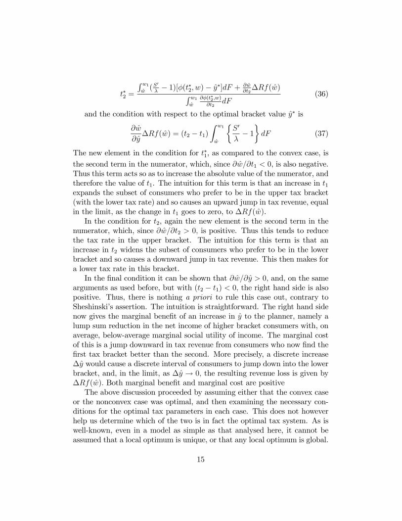
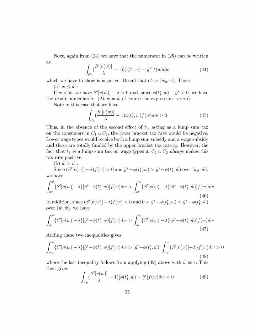
between convex and nonconvex tax systems, we compare each in generalterms with an initially optimal linear tax. Figure 1 illustrates the comparisonbetween the optimal linear tax and the optimal convex two-bracket tax. Theline aLL represents the budget constraint facing all consumers under theoptimal linear tax, aCCD that under the optimal convex piecewise linear tax.Given that each tax system satis�es the government revenue requirement, onebudget constraint cannot lie entirely above the other over the whole domainof y-values. Thus there must be at least one intersection point within thisdomain. Cases however can, by suitable choices of the wage distribution,parameters of the SWF and compensated labour supply elasticities, also beconstructed in which aC � aL; the lump sum transfer is at least as high inthe convex piecewise linear case.Figure 1 about hereThe essential feature of the illustration is that the convex piecewise linear

tax system redistributes welfare towards the middle and away from the ends,as compared to the linear tax, since over the range AB the budget constraintlies above that in the linear case, outside that range it is everywhere belowit. All consumers in the lower tax bracket under the piecewise linear tax willexpand their (compensated) labour supplies, all those in the higher bracket

16

will contract theirs, as compared to the linear tax. However, in the case inwhich optimally aC > aL (not shown), only consumers in the upper part ofthe higher tax bracket would be worse o¤. In this case a higher tax rate inthe upper bracket funds a larger lump sum transfer as well as a lower taxrate in the lower bracket.Figure 2 compares the optimal linear and nonconvex piecewise linear tax

systems. The budget constraint corresponding to the linear tax is again aLL;that of the piecewise linear tax is aNEF: Thus we see that, as compared tothe linear tax, the nonconvex piecewise linear tax redistributes welfare fromthe middle towards the bottom and top. Lower bracket consumers, who nowpay a higher marginal rate, reduce their labour supplies and gross incomes,higher bracket consumers increase theirs. Cases are also possible in whichaN � aL; and so only the upper segment of the higher bracket would bemade better o¤. In this case, a constant or reduced lump sum transfer anda higher tax rate in the lower bracket funds a lower tax rate in the upperbracket. There is a good deal of evidence to suggest that tax reforms over thelast couple of decades in a number of OECD countries, notably the US, UKand Australia, have had this outcome. Tax cuts at the top have, in e¤ect,been funded by higher taxes on the middle, often made less than transparentby expressing the changes in rate structure in terms of an income supplementto the lowest wage types with a high withdrawal rate as a function of incomeover the lower and middle income ranges.21

Figure 2 about here

4.1 A general discrete model

The simplicity of the model presented here means that the e¤ects of changesin the parameters, especially the wage distribution, are very transparent.This contrasts with the study by Slemrod et al., which, following Stern(1976), assumed CES utility functions, a utilitarian SWF22 and a lognormalwage distribution, the parameters of which were taken from Stern, and whichrelate to an estimated wage distribution dating from the late 1960�s/early1970�s. This model was solved for varying values of the elasticity of sub-stitution in the utility function which, as Saez (2001) points out, bear no

21See Apps and Rees (2010), where this is discussed at some length for the case ofAustralia. Similar points apply to the UK and US.22A SWF with a positive degree of inequality aversion was also considered, with no

signi�cant change in results.

17

simple relationship to the compensated labour supply elasticities on whichour intuition is more usually based. No changes in the wage distribution wereconsidered, yet, as our results show, this is in fact the most important driverof the results, as far as the general shape of the tax structure is concerned.Consistent with the theoretical discussion given earlier, we �nd that for

selected values of �; the parameter expressing the planner�s inequality aver-sion, and for plausible elasticities:

� The optimal rate structure is always convex when the wage distributionis at �rst relatively �at and then rises steeply in the higher deciles,implying greater wage and income inequality among these deciles andin the distribution overall, as compared to the distribution used bySlemrod et al. This pattern in fact characterises the existing wagedistributions of fully employed individuals of prime age in many OECDcountries, in particular the US, UK, Germany and Australia.23

� The progressivity of the optimal convex rate scale increases as the in-equality in wage rates among the top deciles increases, as we wouldexpect from the theoretical conditions presented earlier in (25) and(26).

� The nonconvex case is optimal if inequality is concentrated in the bot-tom percentiles and the remainder of the distribution is relatively �at,again as suggested by the theoretical results presented earlier.

� The nonconvex case can also be obtained with the more realistic dis-tribution if we assume an implausibly large gap between elasticities forthe lower and upper parts of the distribution, with a very high elasticityat the top.

In the general discrete model the n household types have gross incomesyi; each corresponding to a wage type wi; i = 1; ::; n; We assume two taxbrackets, and the bracket limit is again denoted by y: The SWF is given by[Pn

i=1 v1��i ]1=(1��); with � 6= 1 a measure of inequality aversion. The indirect

utility functions vi are derived just as in Section 2, with the quasilinear utilityfunction u = x � kl�, � > 1. The parameters k and � are calibrated so asto yield empirically reasonable values of labour supplies and compensated

23See, for example, the distributions of the earnings and hours of primary earners re-ported in Apps and Rees, 2009, Ch 1.

18

labour supply elasticities respectively, given the distributions of wage types.In the solution to the optimal tax problem, each wage type i will have acorresponding labour supply and gross income y�i , increasing in the wage,and we let j denote the type such that y�1 < ::: � y�j � y < y�j+1 < ::: < y�n;that is, the highest wage type in the lower income bracket.We write the optimal tax problem as:

maxa;t1;t2;y

fnXi=1

[vi(a; t1; t2; y)]1��g1=(1��) (38)

s.t. t1

jXi=1

yi(t1) + t2

nXi=j+1

(yi(t2)� y) + (n� j)t1y � na � 0 (39)

We then solve this problem numerically for the optimal lump sum transfera, tax rates t1; t2 and bracket limit y; given assumed parameter values for� and the compensated labour supply elasticity " (which implies a uniquevalue for �), and given the wage distributions that were discussed in generalterms above, and are described in more detail in the next subsection. Thenumerical analysis presented below is based on n = 1; 000: The procedure isto assume successive values of the tax bracket y at $100 intervals throughoutthe income distribution and solve numerically for the optimal tax rates andlump sum transfer at each bracket value. We then take the bracket valuewhich yields the global maximum of the SWF.24

4.2 Numerical Results

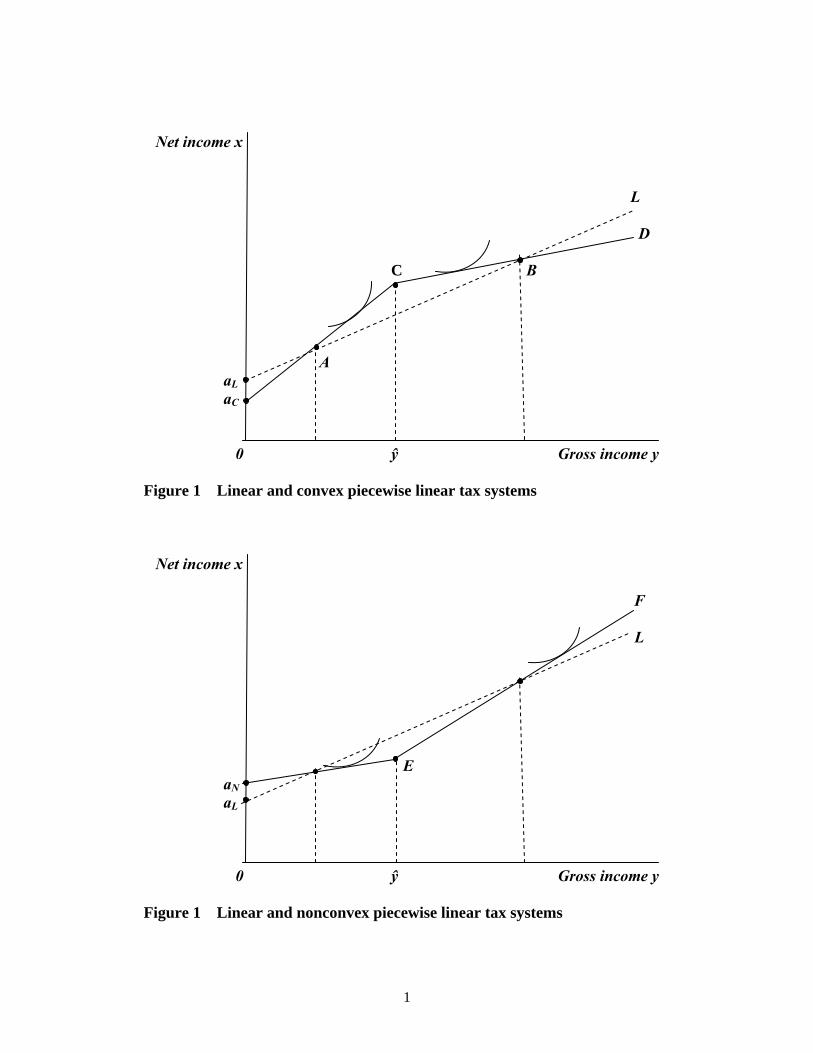
We solve for globally optimal tax structures for two sets of wage distribu-tions.25 In the �rst set we begin with a Pareto wage distribution de�ned toapproximate that of primary earners, aged from 25 to 59 years and earningabove the minimumwage, in a sample of couples selected from a recent house-

24Two methods were used: general grid search and global optimisation software. Theygave virtually identical results.25These distributions were constructed by �rst taking 1 million random draws from a

Pareto distribution with the given parameter, truncated in the way described in the textand arranged into 1000 equally-sized blocks in ascending order of size. The mean of eachblock was then calculated, to give the discrete distribution for 1000 wage types used inthe numerical analysis.

19

hold survey.26 Limiting the sample to primary earners on above minimumwages excludes those on very low earnings and recipients of unemploymentand disability bene�ts, who make up around 20 per cent of the full sample.Wage rates that closely match those of the selected sample are generated bya Pareto distribution27 with a beta parameter of 3.5, a lower bound of $20per hour and an upper bound at the 98th percentile. These parameters setwage rates in the upper percentiles at higher rates than in the data to adjustfor top-end coding. To illustrate the implications of rising top incomes forthe structure of optimal tax rates, we then vary the beta parameter to con-struct two further distributions with lower degrees of inequality in the toppercentiles. Thus we have the following three distributions, which we labelDistribution Set 1:Distribution 1a: � = 3.5. Average wage = $48.10Distribution 1b: � = 2.0. Average wage = $35.03Distribution 1c: � = 1.5. Average wage = $28.34We would argue that the economic circumstances of households in this

type of sample are, at least to some extent, consistent with two assumptionsof optimal tax theory - that productivities are innate and cannot be observedand, therefore, that wage rates representing productivities can be treated asexogenous and unobservable. These assumptions cannot plausibly be con-sidered to hold in the case of recipients of disability pensions or long termunemployment bene�ts. Many types of disabilities are observable and disabil-ity pensions are individual-speci�c and not part of the general tax system. Inthe case of the long term unemployed, the available empirical evidence sug-gests that their earnings possibilities re�ect the need for further education,training and work experience, implying that a broader set of policy instru-ments than income taxation are relevant, and indeed are in use. We thereforeregard the results for the above set of distributions as being the most relevantfor the general analysis of tax systems in present-day economies.To show the extent to which a nonconvex income tax structure can result

from including these categories of welfare recipients, we construct a second

26We draw on data for primary earnings and hours reported for couple income unitrecords in the Australian Bureau of Statistics 2008 Income and Housing Survey.27The cdf of the Pareto distribution for a variate x is given by F (x) = 1� (Ax )

a if x � Aand F (x) = 0 if x < A, with Pareto index a > 1 and parameter � = a=(a� 1): Increasing� is associated with increasing inequality in the distribution.

20

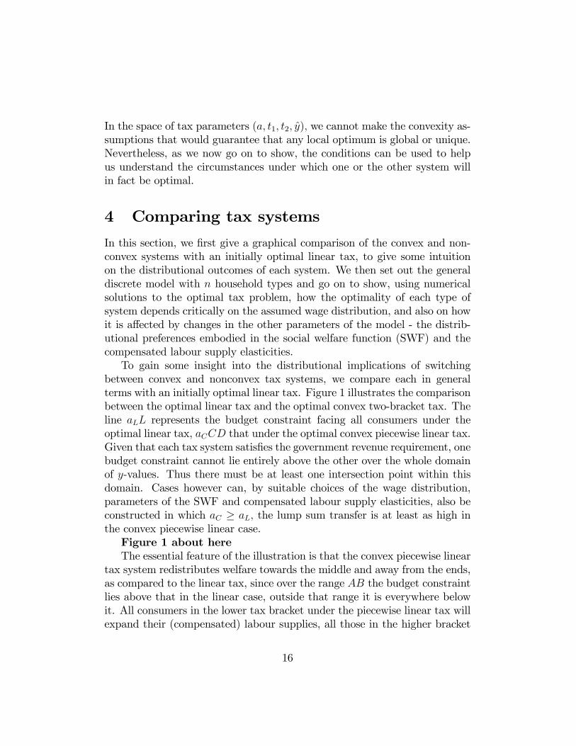
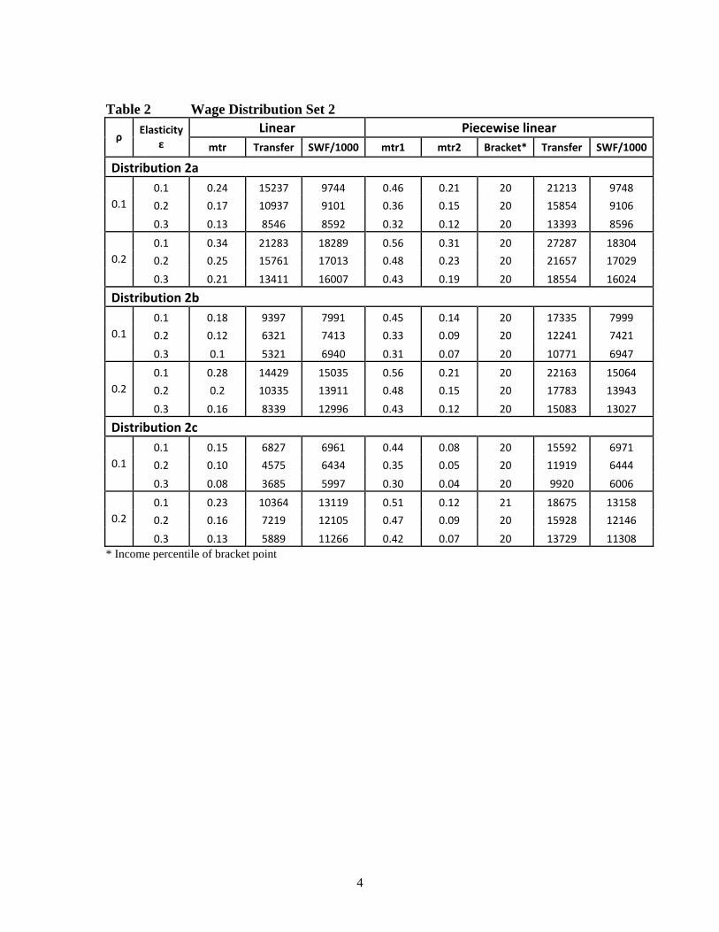
set of three wage distributions, which we label Distribution Set 2. In eachdistribution we allow wage rates to rise steeply in the �rst two deciles andthen become relatively �at, by taking the same Pareto distributions as abovebut combining each with a uniform distribution up to the 20th percentile,a lower bound of $20 at this point and an upper bound at the 90th per-centile. The new distributions show considerable inequality at the bottombut relatively little at the top, in contrast to the actual wage distribution,and represent rising inequality over time. Average wage rates are as follows:Distribution 2a: Average wage = $31.98Distribution 2b: Average wage = $26.29Distribution 2c: Average wage = $22.92Percentile wage distributions for each set are shown in Figures 3a and 3b.Figures 3a and 3b about hereTable 1 reports the optimal tax parameters and bracket points for the �rst

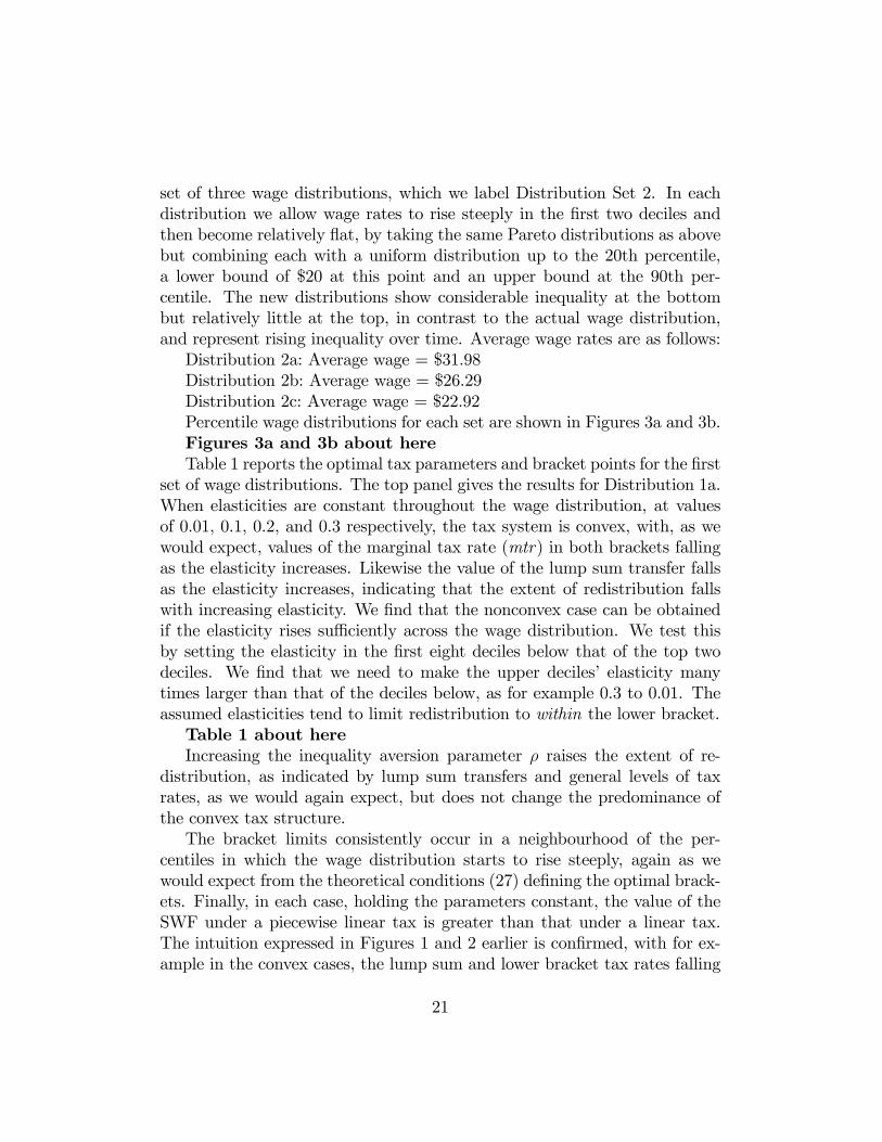
set of wage distributions. The top panel gives the results for Distribution 1a.When elasticities are constant throughout the wage distribution, at valuesof 0.01, 0.1, 0.2, and 0.3 respectively, the tax system is convex, with, as wewould expect, values of the marginal tax rate (mtr) in both brackets fallingas the elasticity increases. Likewise the value of the lump sum transfer fallsas the elasticity increases, indicating that the extent of redistribution fallswith increasing elasticity. We �nd that the nonconvex case can be obtainedif the elasticity rises su¢ ciently across the wage distribution. We test thisby setting the elasticity in the �rst eight deciles below that of the top twodeciles. We �nd that we need to make the upper deciles� elasticity manytimes larger than that of the deciles below, as for example 0.3 to 0.01. Theassumed elasticities tend to limit redistribution to within the lower bracket.Table 1 about hereIncreasing the inequality aversion parameter � raises the extent of re-

distribution, as indicated by lump sum transfers and general levels of taxrates, as we would again expect, but does not change the predominance ofthe convex tax structure.The bracket limits consistently occur in a neighbourhood of the per-

centiles in which the wage distribution starts to rise steeply, again as wewould expect from the theoretical conditions (27) de�ning the optimal brack-ets. Finally, in each case, holding the parameters constant, the value of theSWF under a piecewise linear tax is greater than that under a linear tax.The intuition expressed in Figures 1 and 2 earlier is con�rmed, with for ex-ample in the convex cases, the lump sum and lower bracket tax rates falling

21

signi�cantly and upper bracket tax rates rising, also signi�cantly.28

Comparing the results for the three distributions shows that reducing thedegree of inequality in the underlying wage distribution reduces the generallevel of tax rates and lump sum transfers, i.e. reduces the extent of redistri-bution, but does not change the conclusions on tax structure. The globallyoptimal tax system continues to be piecewise linear and convex, except forthe case in which the top percentiles have an elasticity that is an implausiblyhigh multiple of that of the lower percentiles - thirty times as high in fact. Inthis case, redistribution is taking place within the lower bracket but hardlyat all within the upper bracket, though the high lump sum tax on the upperbracket incomes corresponding to the high lower bracket tax rate helps funda relatively large lump sum transfer, bene�ting the very lowest wage types,as illustrated in Figure 2 earlier.The main di¤erence to the results that arises when we take the second

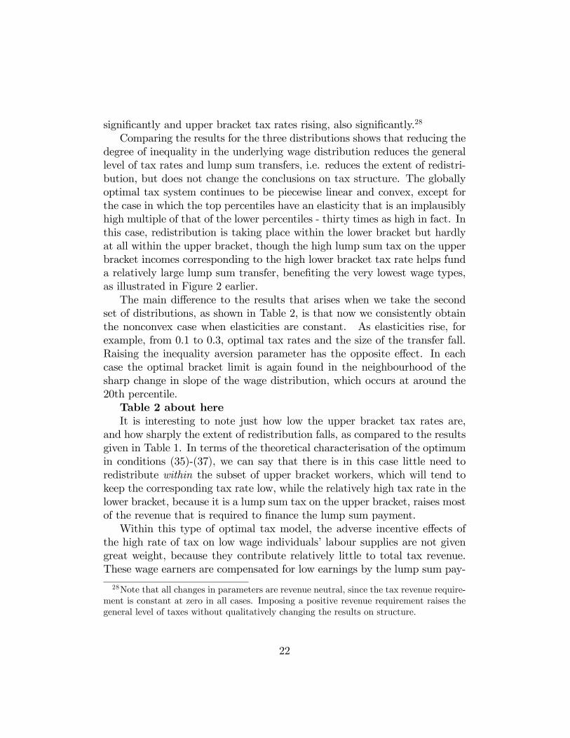
set of distributions, as shown in Table 2, is that now we consistently obtainthe nonconvex case when elasticities are constant. As elasticities rise, forexample, from 0.1 to 0.3, optimal tax rates and the size of the transfer fall.Raising the inequality aversion parameter has the opposite e¤ect. In eachcase the optimal bracket limit is again found in the neighbourhood of thesharp change in slope of the wage distribution, which occurs at around the20th percentile.Table 2 about hereIt is interesting to note just how low the upper bracket tax rates are,

and how sharply the extent of redistribution falls, as compared to the resultsgiven in Table 1. In terms of the theoretical characterisation of the optimumin conditions (35)-(37), we can say that there is in this case little need toredistribute within the subset of upper bracket workers, which will tend tokeep the corresponding tax rate low, while the relatively high tax rate in thelower bracket, because it is a lump sum tax on the upper bracket, raises mostof the revenue that is required to �nance the lump sum payment.Within this type of optimal tax model, the adverse incentive e¤ects of

the high rate of tax on low wage individuals�labour supplies are not givengreat weight, because they contribute relatively little to total tax revenue.These wage earners are compensated for low earnings by the lump sum pay-

28Note that all changes in parameters are revenue neutral, since the tax revenue require-ment is constant at zero in all cases. Imposing a positive revenue requirement raises thegeneral level of taxes without qualitatively changing the results on structure.

22

ment, funded primarily by the lump sum tax on higher wage earners. Thisis con�rmed by the result that when the inequality aversion parameter �increases, the lower bracket mtr also increases signi�cantly, while the lumpsum payment is also sharply higher.In a broader perspective this aspect of the results can be seen as a weak-

ness of this type of optimal tax model. It ignores the longer term issuespresented by having a class of low wage workers facing at the margin veryhigh tax disincentives to work, even though they are compensated in con-sumption terms by a lump sum transfer. Among other things, this can leadto the inter-generational transmission of negative attitudes to work and ac-quisition of labour market quali�cations. It is for this reason that we preferto work in terms of the �rst set of distributions, while arguing that a broaderset of policies is required to deal with the welfare of households which are atthe bottom of the wage distribution for reasons of ill-health or low humancapital.

5 Conclusions

Given its signi�cance in practice, the piecewise linear tax system seems tohave received disproportionately little attention in the literature on optimalincome taxation. This paper contributes a simple and transparent analysisof its main characteristics. An important result is that, contrary to theresults presented by Slemrod et al. (1994), for currently relevant empiricalwage distributions the optimal tax structures consistently show marginal rateprogressivity, giving what we have called here the convex case.We have considered formally only the two bracket case, but it is easy

to see how this can be extended to an arbitrary number of brackets. It istheoretically possible that some portions of the tax system might be convexand some nonconvex, in a way that depends on the characteristics of thewage distribution, the income distributional preferences of the tax policymaker and the way in which labour supply elasticities vary with wage type.We would argue however that the problems presented by very low-wage andlong-term unemployed workers are best addressed through speci�c policiesdirected at these groups, rather than through the design of the general taxstructure.The analysis also provides an interesting perspective on tax policy in a

23

number of countries over the past few decades, in particular in the US, UKand Australia. Cuts in tax rates at the top have been funded by higher taxrates over the range of low-to-middle incomes, and our analysis suggests that,given the substantial increases in wage inequality that have also taken placeover this period, this policy can only be explained either by assumptions ofunrealistically high values of earnings elasticities at the top relative to thoselower down the distribution, or by strong preferences of the "social planner"for redistributing income to the already well-o¤.The question of the optimal number of brackets is left open. Note, how-

ever, that we are not trying to �nd the best piecewise linear approximationto a known nonlinear tax function that is optimal in the sense of Mirrlees, inthat it separates all wage types and o¤ers each a marginal tax rate optimalfor its type. Rather, we start from the position that it is practical only topool all wage types. Given the complexity of the situation which faces theplanner, in which the multi-dimensionality of the type-space rules out thepractical derivation of a Mirrlees-optimal tax function, this may be the onlyfeasible approach to designing real-world tax systems.

Appendix A

Note �rst that, since S 0[v(w)] is strictly decreasing in w, the �rst ordercondition in (24) implies that there exists a �w 2 (w0; w1) such that S 0[v(w)]�� T 0 according as w S �w; for all w 2 [w0; w1]: Then, since f(w) > 0; wehave Z �w

w0

fS 0[v(w)]� �gf(w)dw = 1=2 (40)

and Z w1

�w

fS 0[v(w)]� �gf(w)dw = �1=2 (41)

It then follows thatZ �

w0

fS 0[v(w)]� �gf(w)dw > 0 for all � 2 [w0; w1) (42)

and Z w1

�

fS 0[v(w)]� �gf(w)dw < 0 for all � 2 (w0; w1] (43)

We make use of the result in (48) below.

24

Next, again from (24) we have that the numerator in (25) can be writtenas Z

C0

(S 0[v(w)]

�� 1)[�(t�1; w)� y�]f(w)dw (44)

which we have to show is negative. Recall that C0 = [w0; ~w): Then:(a) ~w � �w :If ~w < �w; we have S 0[v(�w)]� � > 0 and, since �(t�1; w)� y� < 0; we have

the result immediately. (At ~w = �w of course the expression is zero).Note in this case that we haveZ

C0

(S 0[v(w)]

�� 1)�(t�1; w)f(w)dw > 0 (45)

Thus, in the absence of the second e¤ect of t1; acting as a lump sum taxon the consumers in C1 [ C2; the lower bracket tax rate would be negative.Lower wage types would receive both a lump sum subsidy and a wage subsidyand these are totally funded by the upper bracket tax rate t2. However, thefact that t1 is a lump sum tax on wage types in C1 [ C2 always makes thistax rate positive.(b) ~w > �w :Since (S 0[v(w)]��)f(w) > 0 and y���(t�1; w) > y���(t�1; �w) over [w0; �w);

we haveZ �w

w0

fS 0[v(w)]��g[y���(t�1; w)]f(w)dw >

Z �w

w0

fS 0[v(w)]��g[y���(t�1; �w)]f(w)dw

(46)In addition, since (S 0[v(w)]��)f(w) < 0 and 0 < y���(t�1; w) < y���(t�1; �w)over (�w; ~w); we haveZ ~w

�w

fS 0[v(w)]��g[y���(t�1; w)]f(w)dw >

Z ~w

�w

fS 0[v(w)]��g[y���(t�1; �w)]f(w)dw(47)

Adding these two inequalities givesZ ~w

w0

fS 0[v(w)]��g[y���(t�1; w)]f(w)dw > [y���(t�1; �w)]Z ~w

w0

fS 0[v(w)]��gf(w)dw > 0

(48)where the last inequality follows from applying (42) above with ~w � � : Thisthen gives Z

C0

(S 0[v(w)]

�� 1)[�(t�1; w)� y�]f(w)dw < 0 (49)

25

as required.

References

[1] P F Apps and R Rees, 2009, Public Economics and the Household, Cam-bridge: Cambridge University Press.

[2] P F Apps and R Rees, 2010, "Australian Family Tax Reform and theTargeting Fallacy", Australian Economic Review, 43 (2), 153-175.

[3] P F Apps and R Rees, 2011, "Two Extensions to the Theory of OptimalIncome Taxation", mimeo.

[4] A B Atkinson, T Piketty and E Saez, 2011, "Top Incomes in the LongRun of History", Journal of Economic Literature, 49(1), 3-71.

[5] R Boadway, "The Mirrlees Approach to the Theory of Economic Policy",International Tax and Public Finance, 5, 67-81.

[6] B Dahlby, 1998, "Progressive Taxation and the Marginal Social Cost ofPublic Funds", Journal of Public Economics, 67, 105-122.

[7] B Dahlby, 2008, The Marginal Cost of Public Funds, The MIT Press,Cambridge, Mass.

[8] P Diamond and E Saez, 2011, "The Case for a Progressive Tax: FromBasic Research to Policy Recommendations". Journal of Economic Per-spectives (forthcoming)

[9] J A Mirrlees, 1971, �An Exploration in the Theory of Optimum IncomeTaxation�, Review of Economic Studies, 38, 175-208.

[10] S Pudney, 1989,Modelling Individual Choice: The Econometrics of Cor-ners, Kinks and Holes, Basil Blackwells, Oxford.

[11] E Sadka, 1976, "On Income Distribution, Incentive E¤ects and OptimalIncome Taxation, Review of Economic Studies, 261-267.

[12] E Saez, 2001, "Using Elasticities to Derive Optimal Tax Rates", Reviewof Economic Studies, 68, 205-229.

26

[13] E Sheshinski, 1972, �The Optimal Linear Income Tax�, Review of Eco-nomic Studies, 39, 297-302.

[14] E Sheshinski, 1989, "Note on the Shape of the Optimum Income TaxSchedule", Journal of Public Economics, 40, 201-215.

[15] J Slemrod, S Yitzhaki, J Mayshar andMLundholm, 1994, "The OptimalTwo-Bracket Linear Income Tax", Journal of Public Economics, 53, 269-290.

[16] N Stern, 1976, "On the Speci�ation of Models of Optimum Income Tax-ation", Journal of Public Economics, 6, 123-162.

[17] M Strawczinsky, 1988, Social Insurance and the Optimum PiecewiseLinear Income Tax", Journal of Public Economics�69, 371-388.

[18] H R Varian, 1980, "Redistributive Taxes as Social Insurance", Journalof Public Economics�141(1), 49-68.

27

Net income x L D C B A aL aC 0 ŷ Gross income y Figure 1 Linear and convex piecewise linear tax systems Net income x F L E aN aL 0 ŷ Gross income y Figure 1 Linear and nonconvex piecewise linear tax systems

1

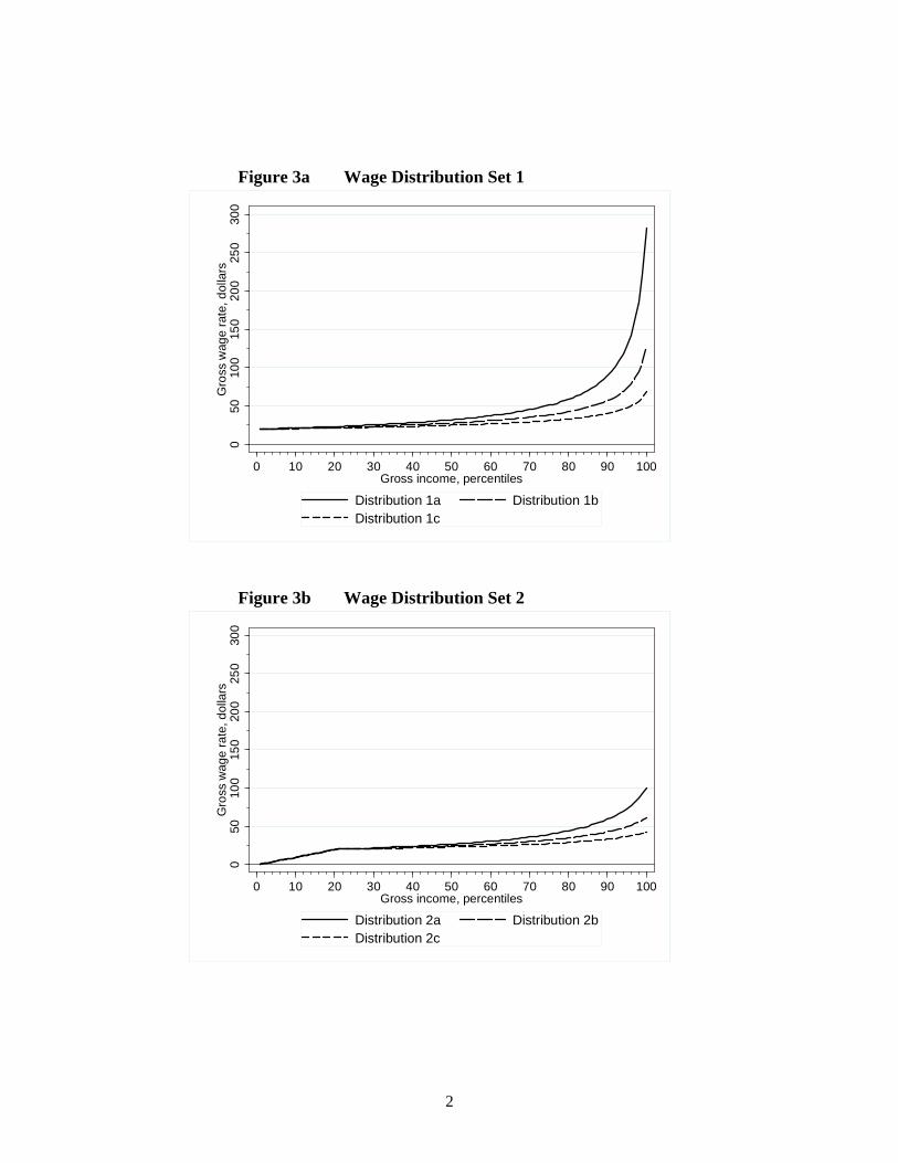
Figure 3a Wage Distribution Set 1

050

100

150

200

250

300

G

ross

wag

e ra

te, d

olla

rs

0 10 20 30 40 50 60 70 80 90 100Gross income, percentiles

Distribution 1a Distribution 1bDistribution 1c

Figure 3b Wage Distribution Set 2

050

100

150

200

250

300

G

ross

wag

e ra

te, d

olla

rs

0 10 20 30 40 50 60 70 80 90 100Gross income, percentiles

Distribution 2a Distribution 2bDistribution 2c

2

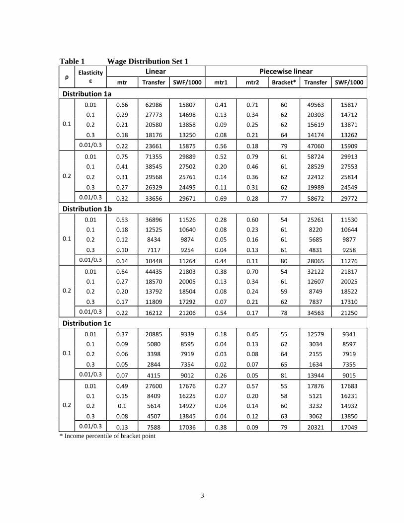
Table 1 Wage Distribution Set 1

Linear  Piecewise linear ρ 

Elasticity ε  mtr  Transfer  SWF/1000  mtr1  mtr2  Bracket*  Transfer  SWF/1000 

Distribution 1a    0.01  0.66  62986  15807  0.41  0.71  60  49563  15817 

   0.1  0.29  27773  14698  0.13  0.34  62  20303  14712 0.1  0.2  0.21  20580  13858  0.09  0.25  62  15619  13871    0.3  0.18  18176  13250  0.08  0.21  64  14174  13262 

   0.01/0.3  0.22  23661  15875  0.56  0.18  79  47060  15909 

   0.01  0.75  71355  29889  0.52  0.79  61  58724  29913 

   0.1  0.41  38545  27502  0.20  0.46  61  28529  27553 0.2  0.2  0.31  29568  25761  0.14  0.36  62  22412  25814 

   0.3  0.27  26329  24495  0.11  0.31  62  19989  24549 

   0.01/0.3  0.32  33656  29671  0.69  0.28  77  58672  29772 

Distribution 1b    0.01  0.53  36896  11526  0.28  0.60  54  25261  11530 

   0.1  0.18  12525  10640  0.08  0.23  61  8220  10644 0.1  0.2  0.12  8434  9874  0.05  0.16  61  5685  9877    0.3  0.10  7117  9254  0.04  0.13  61  4831  9258 

   0.01/0.3  0.14  10448  11264  0.44  0.11  80  28065  11276 

   0.01  0.64  44435  21803  0.38  0.70  54  32122  21817 

   0.1  0.27  18570  20005  0.13  0.34  61  12607  20025 0.2  0.2  0.20  13792  18504  0.08  0.24  59  8749  18522 

   0.3  0.17  11809  17292  0.07  0.21  62  7837  17310 

   0.01/0.3  0.22  16212  21206  0.54  0.17  78  34563  21250 

Distribution 1c    0.01  0.37  20885  9339  0.18  0.45  55  12579  9341 

   0.1  0.09  5080  8595  0.04  0.13  62  3034  8597 0.1  0.2  0.06  3398  7919  0.03  0.08  64  2155  7919    0.3  0.05  2844  7354  0.02  0.07  65  1634  7355 

   0.01/0.3  0.07  4115  9012  0.26  0.05  81  13944  9015 

   0.01  0.49  27600  17676  0.27  0.57  55  17876  17683 

   0.1  0.15  8409  16225  0.07  0.20  58  5121  16231 0.2  0.2  0.1  5614  14927  0.04  0.14  60  3232  14932 

   0.3  0.08  4507  13845  0.04  0.12  63  3062  13850 

   0.01/0.3  0.13  7588  17036  0.38  0.09  79  20321  17049 * Income percentile of bracket point

3

4

Table 2 Wage Distribution Set 2

Linear  Piecewise linear ρ 

Elasticity ε  mtr  Transfer  SWF/1000  mtr1  mtr2  Bracket*  Transfer  SWF/1000 

Distribution 2a    0.1  0.24  15237  9744  0.46  0.21  20  21213  9748 0.1  0.2  0.17  10937  9101  0.36  0.15  20  15854  9106    0.3  0.13  8546  8592  0.32  0.12  20  13393  8596 

   0.1  0.34  21283  18289  0.56  0.31  20  27287  18304 0.2  0.2  0.25  15761  17013  0.48  0.23  20  21657  17029 

   0.3  0.21  13411  16007  0.43  0.19  20  18554  16024 

Distribution 2b    0.1  0.18  9397  7991  0.45  0.14  20  17335  7999 0.1  0.2  0.12  6321  7413  0.33  0.09  20  12241  7421    0.3  0.1  5321  6940  0.31  0.07  20  10771  6947 

   0.1  0.28  14429  15035  0.56  0.21  20  22163  15064 0.2  0.2  0.2  10335  13911  0.48  0.15  20  17783  13943 

   0.3  0.16  8339  12996  0.43  0.12  20  15083  13027 

Distribution 2c    0.1  0.15  6827  6961  0.44  0.08  20  15592  6971 0.1  0.2  0.10  4575  6434  0.35  0.05  20  11919  6444    0.3  0.08  3685  5997  0.30  0.04  20  9920  6006 

   0.1  0.23  10364  13119  0.51  0.12  21  18675  13158 0.2  0.2  0.16  7219  12105  0.47  0.09  20  15928  12146 

   0.3  0.13  5889  11266  0.42  0.07  20  13729  11308 * Income percentile of bracket point