optimal investment and financial strategies under tax-rate uncertainty

Optimal Investment and Financial Strategiesunder Tax-Rate UncertaintyAlessandro FedeleUniversity of Brescia

Paolo M. PanteghiniUniversity of Brescia and CESifo

Sergio VergalliUniversity of Brescia and FEEM

Abstract. In this paper, we apply a real-option model to study the effects of tax-rateuncertainty on a firm’s decision. In doing so, we depart from the relevant literature, whichfocuses on fully equity-financed investment projects. By letting a representative firm borrowoptimally, we show that debt finance not only encourages investment activities but can alsosubstantially mitigate the effect of tax-rate uncertainty on investment timing.

JEL classification: H2.

Keywords: Capital levy; corporate taxation; default risk; real options.

1. INTRODUCTION

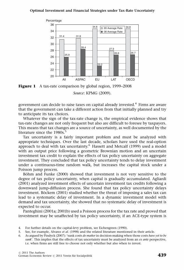
Over the last decades, increase in capital mobility has led to a sharp rise in foreigndirect investments (FDIs) and multinational activity, thereby creating theconditions for international tax competition.1 As shown in Figure 1, among the106 countries surveyed by KPMG (2009), the average of corporate statutory tax rates(All) has fallen from 31.4% to 25.9% over the 1999–2008 period. While tax cutswere less pronounced in Latin American (LAT) and Asian Pacific (ASPAC) countries,much more dramatic tax cuts occurred in industrialized countries: in the EuropeanUnion, for example, the decrease was sharper (i.e. from 34.2% to 23.2%). We cantherefore say that, due to tax competition, firms have been operating in a tax-rate-cut scenario where further reductions might occur in the future.2

Despite these generalized tax-cut policies, the recent world crisis has ledpoliticians to discuss a possible tax-rate increase aimed at financing the policiesimplemented to offset the dramatic effects of the 2008–09 recession.3 As pointedout by Mintz (1995, p. 61): ‘When capital is sunk, governments may have theirresistible urge to tax such a capital at a high rate in the future. This endogeneity ofgovernment decisions results in a problem of time consistency in tax policy, wherebygovernments may wish to take actions in the future that would be different fromwhat would be originally planned’. In this case, the commitment failure leads tothe well-known ‘capital-levy problem’, which is related to a firm’s fear that a

1. See, for example, Devereux et al. (2008) and Ghinamo et al. (2010).2. KPMG experts add that ‘we have found no country anywhere that has raised its rate since last year’

(KPMG, 2009, p. 6).3. The sharp increase in public deficits throughout the world will probably be tackled not only by

cutting public spending but also by increasing tax rates. Some US states (such as Oregon and Illinois)have already planned or are planning to raise statutory tax rates. Similarly, public budget concernsin the eurozone make tax rate increases more likely in some countries.

r 2011 The AuthorsGerman Economic Review r 2011 Verein fur Socialpolitik. Published by Blackwell Publishing Ltd, 9600Garsington Road, Oxford OX4 2DQ, UK and 350 Main Street, Malden, MA 02148, USA.

German Economic Review 12(4): 438–468

government can decide to raise taxes on capital already invested.4 Firms are awarethat the government can take a different action from that initially planned and tryto anticipate its tax choices.

Whatever the sign of the tax-rate change is, the empirical evidence shows thattax-rate changes are not only frequent but also are difficult to foresee by taxpayers.This means that tax changes are a source of uncertainty, as well documented by theliterature since the 1980s.5

Tax uncertainty is a fairly important problem and must be analyzed withappropriate techniques. Over the last decade, scholars have used the real-optionapproach to deal with tax uncertainty.6 Hassett and Metcalf (1999) used a modelwith an output price following a geometric Brownian motion and an uncertaininvestment tax credit to explain the effects of tax policy uncertainty on aggregateinvestment. They concluded that tax policy uncertainty tends to delay investmentunder a continuous-time random walk, but increases the capital stock under aPoisson jump process.

Bohm and Funke (2000) showed that investment is not very sensitive to thedegree of tax policy uncertainty, when capital is gradually accumulated. Agliardi(2001) analyzed investment effects of uncertain investment tax credits following adownward jump-diffusion process. She found that tax policy uncertainty delaysinvestment. Bockem (2001) studied whether the threat of imposing a sales tax canlead to a systematic delay of investment. In a dynamic investment model withdemand and tax uncertainty, she showed that no systematic delay of investment isexpected to occur.

Panteghini (2001a; 2001b) used a Poisson process for the tax rate and proved thatinvestment may be unaffected by tax policy uncertainty, if an ACE-type system is

31.4 31.8

34.8

27.9

34.8

25.9

28.4

23.2

26.6 26.7

20

22

24

26

28

30

32

34

36

All ASPAC EU LAT OECD

99 Average Rate08 Average Rate

Percentage

Figure 1 A tax-rate comparison by global region, 1999–2008

Source: KPMG (2009).

4. For further details on the capital-levy problem, see Eichengreen (1990).5. See, for example, Alvarez et al. (1998) and the related literature mentioned in their article.6. As argued by Pindyck (2007): ‘sunk costs do matter in decision-making when those costs have yet to be

sunk’. This implies that the effects of tax uncertainty must be analyzed from an ex ante perspective,i.e. when firms are still free to choose not only whether but also when to invest.

Optimal Investment and Financial Strategies under Tax-Rate Uncertainty

r 2011 The AuthorsGerman Economic Review r 2011 Verein fur Socialpolitik 439

applied. Niemann (2004) defined two neutrality conditions: first-order neutrality,which requires the complete ineffectiveness of taxation on investment decisions;second-order neutrality, which means that the stochastic nature of taxation doesnot alter investment decisions. In a subsequent article (Niemann, 2006), heanalyzed combined tax-rate and tax-base uncertainty by assuming a stochastic taxpayment. He showed that the uncertainty of tax payments has an ambiguousimpact on investment timing.7 Recently, Chen and Funke (2008) have found thatpolitical uncertainty (including discontinuous changes in taxation) discourages FDIdecisions.

It is worth noting that all these articles deal with tax uncertainty by assumingfully equity-financed investment decisions. However, the evidence shows thatinvestment and financial decisions are related and, hence, should be jointlyanalyzed. To provide a more realistic analysis, therefore, we depart from therelevant literature and let a firm borrow optimally. Given the importance that thestatutory tax rate has on financial choices (see, e.g., Leland, 1994), we will focus ontax-rate uncertainty. Moreover, since the evidence shows that tax-rate changes arediscrete, we will describe them with a Poisson process. In doing so, we will be ableto study two possible scenarios: a standard capital-levy one, where the tax rate isexpected to rise, and a tax-competition one, where there is a downward trend in taxrates.

Given this model, we will study investment and financing decisions jointly. Aswill be shown, debt finance not only encourages investment activities but also cansubstantially mitigate the effect of tax-rate uncertainty on investment timing. Inparticular, using a numerical simulation, based on realistic parameter values, wewill show that a highly volatile tax system may have a negligible impact oninvestment choices, if firms can choose their capital structure. If, however, they arecredit constrained, the impact of tax-rate uncertainty is much more significant. Ourresults have implications in terms of both empirical analysis and policy decisionmaking. First, we can say that econometric investigation should control for theexistence (absence) of financial flexibility. Otherwise, estimates would be mislead-ing. Second, the effects of a hot policy debate on future (and uncertain) tax-ratechanges crucially depend on the efficiency of the financial market and, inparticular, on the existence/absence of credit constraints.

The structure of the paper is as follows. Section 2 describes the model. Section 3shows our main findings and discusses how tax-rate uncertainty affects a firm’schoices. Section 4 makes a comparison with the results obtained in the relevantliterature, and then discusses the implications of our findings. After a briefsummary, Section 5 discusses some possible extensions that are left for futureresearch.

2. THE MODEL

In this section we introduce an earning before interest and taxes (EBIT)-basedmodel in the spirit of Goldstein et al. (2001). By focusing on cash flows rather thanstocks, we can better describe the investment and financial strategies of aninfinitely lived risk-neutral firm.8

7. On this point, see also Sureth (2002).8. For a study on risk-averse firms’ investment choices, see Niemann and Sureth (2004; 2005).

A. Fedele et al.

r 2011 The Authors440 German Economic Review r 2011 Verein fur Socialpolitik

Let us denote Pt as the firm’s EBIT at time t and assume that it evolves as follows

dPt

Pt¼ adt þ sdzt ; with P0 > 0 ð1Þ

where a is the expected rate of growth, s is the instantaneous standard deviation ofdPt=Pt and dzt is the increment of a Brownian motion. Moreover, let us introducethe following hypotheses.

Assumption 1. The firm must pay a sunk start-up cost, denoted by I, to undertakea risky project.

Assumption 2. The firm can borrow from a perfectly competitive risk-neutralcredit sector, characterized by a given risk-free interest rate r.

Assumption 3. The firm can decide how much to borrow by choosing a non-renegotiable coupon C.

Assumption 4. Default takes place when Pt goes to C.

Assumption 5. The cost of default is equal to uC with u40.

According to Assumption 1, the firm must pay a sunk cost. This means thatinvestment projects are irreversible. Assumption 2 entails a simple frameworkwhere lenders are price-takers and become shareholders in the event of default. Inline with Leland (1994), the firm chooses an optimal coupon (Assumption 3).9 Forsimplicity, the capital structure is assumed to be static, i.e. financial policy cannotbe reviewed later.10 Moreover, according to Assumption 4, default occurs when thefirm’s profit, net of its debt obligations, is nil.11 The existence of some defaultcost is necessary to obtain a finite optimal debt-equity ratio.12 For this reason weassume that, when default takes place, a sunk default cost, equal to uC, is faced(Assumption 5).13

9. Given C and the risk-free interest rate r, the market value of debt can be calculated. It is worthnoting that, in the absence of arbitrage, setting the coupon first, and then calculating the marketvalue of the debt is equivalent to first choosing the value of the debt and then calculating theeffective interest rate. The ratio between C and the market value of the debt is equal to the effectiveinterest rate (which is given by the sum between r and the default risk premium).

10. Ruling out the option to renegotiate debt does not affect the qualitative properties of the model.For a detailed analysis of dynamic tradeoff strategies, with costly debt renegotiation, see, forexample, Goldstein et al. (2001), and Hennessy and Whited (2005).

11. Assumption 4 implies that debt is protected. As pointed out by Leland (1994), minimum net-worthrequirements, implied by protected debt, are common in short-term debt financing. For furtherdetails on default conditions, see Brennan and Schwartz (1977), and Smith and Warner (1979). Fora comparison between protected and unprotected debt financing, see also Panteghini (2007a).

12. For further details on this point, see Leland (1994) and Amaro de Matos (2001, Ch. 2).13. The quality of results does not change if, like Leland (1994), we assume that default costs are

proportional to a firm’s value.



Let us next introduce taxation. We define t as the tax rate and assume thatinterest payments are fully deductible. As to the treatment of the lender’s receipts,the evidence shows that effective tax rates on capital income are fairly low. Forsimplicity, therefore, we disregard personal taxation and assume that the lender’spredefault tax burden is nil, so that her after-tax profit function at any instant t issimply C.14 When, however, default takes place, the lender becomes a shareholderand is then subject to corporate taxation.

Given these assumptions a firm’s after-tax profit function, at time t, is equal to

PNt ¼ 1� ttð Þ Pt � Cð Þ ð2Þ

Given Assumption 4, therefore, default takes place when PtN 5 0. This means that

the default threshold point is C.Let us finally model tax-rate uncertainty. We assume that the tax rate follows a

Poisson process. Given an initial tax rate t0, at any short time interval dt there is aprobability ldt that the tax rate changes to t1 (9 t0). Hence, we can write

dt ¼ 0 w:p: 1� ldtDt w:p: ldt

�ð3Þ

where Dt5 t1� t0. Given (3), we can therefore focus on:

1. a capital-levy scenario, where the tax rate is expected to rise (i.e. Dt40);2. a tax-competition scenario, where the tax rate is expected to decrease (i.e.

Dto0).

In order to study a firm’s choices, we need to calculate both its value function, i.e.its net present value (NPV) (for a given level of P) and its option value, i.e. the valueof its option to delay investment (see Dixit and Pindyck, 1994): we will define themas Vi( � ) and Oi( � ), respectively. Subscript i is equal to 0 (1) when t5 t0 (t5 t1). Usingdynamic programming, we will calculate these functions as the summationbetween the current profit (if any) earned in the short interval dt and theremaining value, that is, the value after the instant dt has passed. For simplicity,hereafter we will omit the time variable t.

2.1. The value function

To keep the model as simple as possible, let us assume that there is no agencyconflict between equityholders and bondholders. This means that financial andreal decisions are made to maximize total firm value.15 Using a backward approach,we will first focus on the value function after the tax-rate change: in this case therelevant rate is t1 and the value function will be denoted by V1(P; C). Subsequently,we will focus on the before-tax-change scenario, where the current statutory rateis t0.

14. This simplifying assumption is in line with Graham and Harvey (2001, p. 190), who find ‘very littleevidence that executives are concerned about . . . personal taxes’ when they run business plans(including financial decisions).

15. If an agency conflict were introduced, managers could be induced to maximize levered equityvalue at the expenses of bondholders (see Jensen and Meckling, 1976; Mauer and Ott, 2000; Mauerand Sarkar, 2005; Myers, 1977). We leave this important extension for future research.

A. Fedele et al.


2.1.1. After the tax-rate change

The value function V1(P; C) is given by the sum between the equity value E1(P; C)and the debt value D1(P; C), net of the investment cost I. As shown in AppendixA.1, it amounts to

V1ðP; CÞ ¼1�t1ð ÞP

d � I; after default1�t1ð ÞP

d þ t1Cr �

t1

r þ u� �

C PC

� �b2 � I; before default

(ð4Þ

where d � r� a40 is the so-called ‘dividend yield’.16 In line with Leland (1994; 1998),therefore, total firm value is equal to the value of assets, plus the value of tax benefitsfrom debt, less the value of potential default costs. This value function includes thebenefits and costs in all future periods. Function (4) is based on an extended versionof Modigliani and Miller (1958; 1963). If we compare (4) with Modigliani and Miller’s(1963, p. 436) formula (3) we can say that 1� t1ð ÞP=d is the value of the unleveredfirm. Similarly, Modigliani and Miller (1963) account for the tax benefit arising fromdebt financing. However, (4) contains the additional term ðt1=rÞ þ u½ �C P=Cð Þb2 , whichmeasures the contingent cost of default. This means that a firm not only faces a sunkcost uC but also loses the tax benefit of interest deductibility (t1C=r). The presentvalue of the default cost is multiplied by P=Cð Þb2, with b2o0 (see Appendix A), whichmeasures the contingent value of 1h in the event of default.

2.1.2. Before the tax-rate change

Let us now calculate the value function before the tax-rate change, V0(P; C). Asshown in Appendix A.2, V0(P; C) is given by the sum of the equity value E0(P; C)and the debt value D0(P; C) before the tax-rate change, net of the investment cost I,i.e.

V0ðP; CÞ ¼ E0ðP; CÞ þD0ðP; CÞ � I

¼ V1 P; Cð Þ þ X P; Cð Þ þ Y P; Cð Þ � I ð5Þ

where

X P; Cð Þ � E0 P; Cð Þ � E1 P; Cð Þ

¼ t1 � t0ð Þ Pdþ l

� C

r þ l

� ��

� C

dþ l� C

r þ l

� �PC

� �b2 lð Þ#

and

Y P; Cð Þ � D0 P; Cð Þ �D1 P; Cð Þ

¼ t1 � t0ð Þ C

dþ lPC

� �b2 lð Þ

16. The relevant discount rate of the first term is d � r. This means that the present value of future cashflow accounts for the expected growth rate a � 0 of P.



are the expected changes in the equity and debt value, respectively. The termP=Cð Þb2 lð Þ, with b2(l)o0 (see Appendix A), is the contingent value of 1h, under tax-

rate uncertainty. As can be seen, the relevant discount rates are dþ l and rþ l(instead of d and r), respectively. This is due to the fact that, before the tax-ratejump, present value calculations must account for the probability l of this taxchange.

It is worth noting that b2(l) depends on the probability of the tax-rate change.This implies that the contingent value of default is affected by tax uncertainty. Tounderstand this important effect, let us compare the tax-uncertainty case with thetax-certainty one. Since b2(l)ob2o0, the inequality P=Cð Þb2 > P=Cð Þb2 lð Þ holds.This means that the contingent value of 1h under tax-rate uncertainty is less thanthat under tax-rate certainty.

Both the expected changes in the equity and debt value account for the tax-ratechange and are proportional to the differential (t1� t0). In particular, X(P; C) isgiven by the product between the tax-rate differential (t1� t0) and the term insquare brackets, which measures the contingent value of equity: this term is givenby the difference between a firm’s equity value, with zero default risk, i.e.P=ðdþ lÞ� � ½C=ðr þ lÞ½ �, and the contingent value of equity in the event of default,i.e. ðC=ðdþ lÞÞ � ðC=ðr þ lÞÞ½ � P=Cð Þb2 lð Þ. Function Y(P; C) measures the impact ofthe tax-rate change on the benefit of interest deductibility. It is thus equal to theproduct between the tax-rate differential (t1� t0) and the contingent value of Ch

(i.e. C P=Cð Þb2 lð Þ), divided by the relevant discount rate (dþ l).

2.2. The option value

Let us next deal with the option to invest. Accordingly, we denote the option valueO1(P; C) and O0(P; C), under tax-rate certainty and uncertainty, respectively.Again, we will follow a backward approach.


Let us start with the after-change scenario. Since the tax-rate change has alreadyoccurred, policy uncertainty has vanished. As shown in Appendix B.1, the optionfunction is equal to

O1 P; Cð Þ ¼ H1Pb1 ð6Þ

where H1 is an unknown. To calculate H1, we denote �P as the entry threshold levelabove which investment is undertaken, and apply the value matching condition(see Dixit and Pindyck, 1994)

V1ðP; CÞjP¼ �P ¼ O1 P; Cð ÞjP¼ �P ð7Þ

Substituting (4) and (6) into (7) and H1 gives

H1 ¼ V1ð �P; CÞ �P�b1 ¼

¼ 1� t1ð Þ �Pd

þ t1C

r� t1 þ ruð ÞC

r

�PC

� �b2

� I

" #�P�b1 ð8Þ

A. Fedele et al.


Substituting (8) into (6) and rearranging gives

O1 P; C; �Pð Þ ¼ P�P

� �b1 1� t1ð Þ �Pd

þ t1C

r

�

� t1 þ ruð ÞCr

�PC

� �b2

� I

#; with P< �P ð9Þ

If, therefore, P< �P, it is optimal for a firm to delay investment rather than toexercise its real option immediately. If, however, PZ �P, the optimal strategy is toinvest immediately. As can be seen, the option value is given by the productbetween P= �Pð Þb1 , i.e. the present value of 1h contingent on the entry decision, and

1� t1ð Þ �Pd

þ t1C

r� t1 þ ruð ÞC

r

�PC

� �b2

� I

" #

that is, the NPV at point P ¼ �P (i.e. when the investment project is optimallyundertaken).


The option value under tax-rate uncertainty can be written as follows (see AppendixB.2)

O0 P; C; bP; �P�

¼ O1 P; C; �Pð Þ þ Z P; C; �P; bP� ð10Þ

where bP is the threshold point. Again, if P< bP, it is optimal to delay investment.The opposite is true for PZbP. Function

Z P; C; �P; bP� ¼ V0

bP; C�

� V1ð �P; CÞbP�P

!b1

24 35 PbP� �b1 lð Þ

ð11Þ

measures the contingent effect of tax-rate uncertainty on the option value (see

Appendix B). Terms V0bP; C�

and V1ð �P; CÞ are the value functions at the relevant

threshold levels bP and �P, respectively, and P=bP� b1 lð Þis the contingent value of 1h

invested when P reaches bP. Finally, bP= �P� b1

measures the impact of tax-rate

uncertainty on the contingent evaluation of assets.It is worth remarking that if �P< bP tax-rate uncertainty delays the investment,

while the opposite is true if �P> bP. As will be shown, a delay (anticipation) will takeplace if Dt40 (Dto0).17

17. Note that, without tax-rate uncertainty, the equality bP ¼ �P holds and therefore bP= �P� b1 ¼ 1.



2.3. The firm’s problem

Given the NPV and the option value, let us next analyze a firm’s decision on boththe coupon C and the investment timing. Again, we will start with the after-taxreform, and then focus on the before-tax-rate change case.


If the tax-rate change has already occurred, a firm’s problem is one of choosing boththe optimal investment trigger point �P*

1 and the optimal coupon �C1. This result canbe obtained by maximizing (9) with respect to �P and C, i.e.18

max�P>0;C>0

P�P

� �b1 ð1� t1Þ �Pd

þ t1C

r� ðt1 þ ruÞC

r

�PC

� �b2

�I

" #ð13Þ

Solving problem (13) gives (Appendix C.1)

�P*1 ¼

1

1þm1

b1

b1 � 1

rI

1� r1;

with m1 �t1

1� t1

b2

b2 � 1

1

1� b2

t1

t1 þ ru

� �� 1b2

> 0

�C1 ¼1

1� b2

t1

t1 þ ru

� �� 1b2

�P*1 ð14Þ

The threshold point �P*1 is given by the product between the term 1=ð1þm1Þ,

which measures the effect of dept financing on the firm’s trigger point, and½b1=ðb1 � 1Þ�½rI=ð1� t1Þ�, which is the value of the threshold point under full-equityfinance (see Panteghini, 2007a; 2007b). Since 1=ð1þm1Þ< 1, debt financingencourages investment (namely includes a firm to invest earlier). The reasoningbehind this result is straightforward: if a firm can borrow, it will invest earlier inorder to benefit from interest deductibility (Panteghini, 2007b).

18. Note that there is an alternative approach to solving the firm’s maximization problem. First, weshould remember that the firm aims at borrowing in order to maximize its value. This means thatat point P ¼ �P the firm chooses the optimal coupon by means of the following first-ordercondition

›V1ðP; CÞ›C

P¼ �P

¼ 0 ð12Þ

with ð›V21 ðP; CÞ=›C2Þ

P¼ �P < 0. Second, in line with Dixit and Pindyck (1994), both the value

matching condition (VMC) and the smooth pasting condition (SPC) must be applied, i.e.

V1ðP; CÞjP¼ �P ¼ O1 P; Cð ÞjP¼ �P

›V1ðP; CÞ›P

P¼ �P

¼ ›O1ðP; CÞ›P

P¼ �P

where the first one is equal to (7). Therefore, a three-equation system with three unknowns isobtained and can be solved. It is worth noting that its solution is the same as that obtained in ourmodel. In both cases, equation (7) is applied. Moreover, the first-order condition of (13) w.r.t. Ccoincides with (12). Finally, the SPC is equal to the first-order condition of problem (13) w.r.t. �P.Since equations are the same, we find the same solutions for the investment trigger point �P*

1 , theoptimal coupon �C1 and the parameter value H1.

A. Fedele et al.


The optimal coupon �C1 is obtained by equating the marginal tax benefit of debtfinancing to the marginal cost of default. As can be seen, the optimal coupon isproportional to the threshold point �P*

1 ; and, hence, to the investment cost I. Asshown in Appendix C.2, both �P*

1 and �C1 are increasing in t1. The positive effect oft1 on the threshold point �P*

1 is due to the fact that the higher the tax rate, thegreater the option value is (i.e. the higher the opportunity cost of immediateinvestment is), and the lower the after-tax value of the project is. Both effects causea delay in investment. The positive sign of › �C1=›t1 means that the higher the ratet1, the greater the benefit of interest deductibility, the higher the optimal coupon is.As shown in Panteghini (2007a), › �C1=›u< 0: This means that an increase in u raisesthe expected cost of default, and, therefore, discourages borrowing.19

Moreover, we can show (see Appendix C.2) that the ratio �C1= �P*1 is increasing in

t1 and decreasing in u. This means that a higher tax rate entails a higher tax benefit,and, therefore, stimulates borrowing for any given level of EBIT. The opposite is truefor u: a higher default cost raises the marginal cost of borrowing, and, therefore,reduces the ratio �C1= �P*

1 .


Under tax-rate uncertainty and before investment, a firm’s problem is as follows

maxbP>0;C>0

O0 P; C; bP; �P�

ð15Þ

where O0 P; C; bP; �P�

is defined by (9)–(11). Solving (15) gives the following first-order conditions

›O0 P; C; bP; �P�

›bP ¼V1ð �P; CÞ P�P

� �b1 b1 lð Þ � b1bP PbP� �b1 lð Þ�b1

þ›V0

bP; C� ›bP PbP

� �b1 lð Þ24

� b1 lð ÞbP V0bP; C� PbP

� �b1 lð Þ#¼ 0 ð16Þ

and

›O0 P; C; bP; �P�

›C¼ ›V1ð �P; CÞ

›C

P�P

� �b1

1� PbP� �b1 lð Þ�b1

" #

þ›V0

bP; C� ›C

PbP� �b1 lð Þ

24 35 ¼ 0 ð17Þ

bP* and C* are the solutions of systems (16) and (17). Although equations (16) and(17) have no closed-form solution, their analysis gives us some hint about the

19. For further details, see Leland (1994).



effects of tax-rate uncertainty. To do so, let us start with the tax-certainty scenario.Setting l5 0 yields b1 lð Þjl¼0 ¼ b1, and therefore, the terms

V1ð �P; CÞ P�P

� �b1 b1 lð Þ � b1bP PbP� �b1 lð Þ�b1

ð18Þ

and

›V1ð �P; CÞ›C

P�P

� �b1

1� PbP� �b1 lð Þ�b1

" #ð19Þ

go to zero. In this case the two-equation system (16) and (17) collapses to the tax-rate-certainty system (C1) and (C2) (in Appendix C.1), with the relevant tax rate t0.

This first step allows us to show that terms (18) and (19) measure the distortionscaused by tax-rate uncertainty. In particular, term (18) measures the marginaldistortion on the threshold EBIT level. As can be seen, (18) is proportional to the

firm’s value after the tax-rate change V1ð �P; CÞ: Moreover, it depends on both

P= �Pð Þb1 and P=bP� b1 lð Þ�b1

: while the former measures the contingent value of 1h

invested when P reaches �P, i.e. when it is optimal to invest in the absence of tax-rate uncertainty, the latter measures the wedge on contingent evaluation due to

tax-rate uncertainty. As we can see, the wedge P=bP� b1 lð Þ�b1

depends on the tax-

rate-uncertainty trigger point bP and on the difference [b1(l)� b1]. This means thatthe higher the parameter l, the larger the tax-rate-uncertainty wedge is, or,equivalently, the greater the distortion caused by tax-rate uncertainty.

A similar reasoning holds for term (19), which enters equation (17). As can beseen, the marginal condition on the coupon depends on the marginal benefit of

debt financing, after the tax-rate change (i.e. ›V1ð �P; CÞ=›C). Moreover, it is

proportional to the contingent value of 1h invested when P reaches �P (i.e.

P= �Pð Þb1 ). Finally, it depends on the tax-rate-uncertainty wedge P=bP� b1 lð Þ�b1

.

Note that P=bP� b1 lð Þ�b1

has two opposing effects on equations (16) and(17): while it raises the left-hand side of (16), it reduces the left-hand side of (17).As will be shown in the next section, this opposing effect will lead to an increase inthe marginal cost of immediate investment and, at the same time, a drop in themarginal cost of debt finance.

3. A NUMERICAL ANALYSIS

In order to analyze how a firm’s ability to borrow affects investment decisions, letus compare the tax-uncertainty scenario with the tax-certainty one. In both cases,we assume that the starting tax rate is t0. While in the tax-certainty case it will beunchanged, under tax-rate uncertainty this rate is expected to jump (either up ordown).

Under tax-rate certainty, the firm’s problem is equivalent to (13), with theassumption that, here, the relevant tax rate is t0 (instead of t1). Hence, its solutions

A. Fedele et al.


will have the same form as solution (14)

�P*0 ¼

1

1þm0

b1

b1 � 1

rI

1� t0

�C0 ¼1

1� b2

t0

t0 þ ru

� �� 1b2 �P*

0

m0 �t0

1� t0b2

b2 � 1

1

1� b2

t0

t0 þ ru

� �� 1b2

> 0 ð20Þ

Obviously, the comparative statics results of Appendix C.2 on solutions (14) holdalso for solutions (20). In other terms, the threshold point and the optimal couponof (20), as well as the ratio �C0= �P*

0 are increasing in the tax rate t0.As pointed out, the tax-rate-uncertainty problem (15) has no closed-form

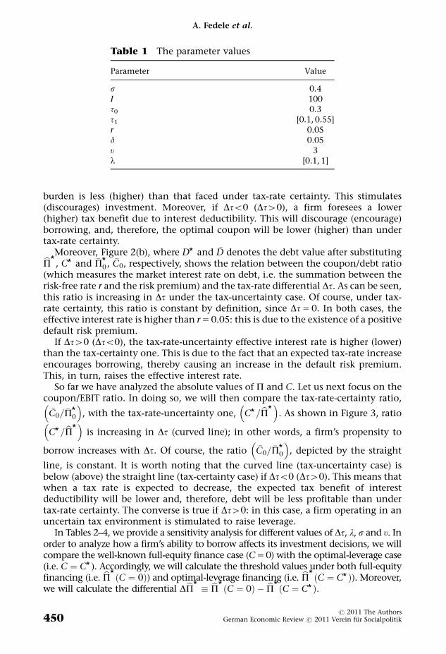
solution. For this reason, we need a numerical analysis to compare the tax-certaintywith the tax-uncertainty case. In doing so, we will use the benchmark parametervalues of Table 1. In line with Dixit and Pindyck (1994, p. 157; 1999, p. 193) we setr 5 d5 0.05 and s5 0.4.20 Furthermore, we assume that u5 3. This means that,given r 5 0.05, the default cost is about 10% of the debt value.21

As we have seen in Figure 1, over the last decade, the average statutory tax ratehas been about 30%. Accordingly, we set t0 5 0.3. Given the high heterogeneity ofthe tax-rate jumps occurring over the past decade, we will assume that t1 rangesfrom 0.1 to 0.55.22 We will therefore be able to study both the capital-levy and thetax-competition case.

Finally, letting l range from 0.1 to 1 entails that the expected time ranges fromx[T] 5 1 (with l5 1) and x[T] 5 10 (with l5 0.1).23

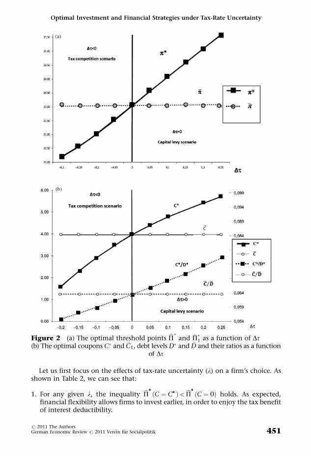
Let us first look at the effects of the tax-rate differential Dt on both the thresholdpoint and the optimal coupon. Figures 2(a) and (b) show that both bP* and C* arepositively affected by the tax-rate differential Dt. The reasoning behind this result isas follows. An increase in Dt means that, given t0 and l, a higher average tax rate(which must account for both the current rate t0 and the expected future one t1) willbe levied. The heavier the expected tax burden, the higher the investment triggerpoint is (i.e. the later the investment will be undertaken). Similarly, an increase in Dtraises the optimal coupon C* . This is due to the fact that a higher average tax rateleads to a higher tax benefit of interest deductibility, thereby encouraging borrowing.

Figures 2(a) and (b) also compare the tax-rate-certainty case (i.e. when Dt5 0)with the tax-rate-uncertainty one (i.e. with Dt6¼0). In particular, if a tax cut isexpected to occur (Dto0) at time x[T] 5 1/l, both the threshold point and theoptimal coupon are less than the tax-rate-certainty ones. The opposite is true ifDt40. This effect can be explained as follows: if Dto0 (Dt40), the expected tax

20. The quality of results does not change if we use different values of s. For further details see, forexample, Leland (1994).

21. This percentage is in line with Branch’s (2002) estimates.22. Of course, the quality of results does not change if a different value of t0 is assumed.23. As shown by Dixit and Pindyck (1994, p. 170), the expected time T of the tax-rate change is equal

to x T½ � ¼R1

0 lTe�lTdT ¼ 1=l. If, therefore, l goes to zero, then x[T] goes to infinity and therelevant tax rate is always t0. If, however, l goes to infinity, the tax-rate change immediately occursand the relevant tax rate will be t1 forever.



burden is less (higher) than that faced under tax-rate certainty. This stimulates(discourages) investment. Moreover, if Dto0 (Dt40), a firm foresees a lower(higher) tax benefit due to interest deductibility. This will discourage (encourage)borrowing, and, therefore, the optimal coupon will be lower (higher) than undertax-rate certainty.

Moreover, Figure 2(b), where D* and �D denotes the debt value after substitutingbP* , C* and �P*0 , �C0, respectively, shows the relation between the coupon/debt ratio

(which measures the market interest rate on debt, i.e. the summation between therisk-free rate r and the risk premium) and the tax-rate differential Dt. As can be seen,this ratio is increasing in Dt under the tax-uncertainty case. Of course, under tax-rate certainty, this ratio is constant by definition, since Dt5 0. In both cases, theeffective interest rate is higher than r 5 0.05: this is due to the existence of a positivedefault risk premium.

If Dt40 (Dto0), the tax-rate-uncertainty effective interest rate is higher (lower)than the tax-certainty one. This is due to the fact that an expected tax-rate increaseencourages borrowing, thereby causing an increase in the default risk premium.This, in turn, raises the effective interest rate.

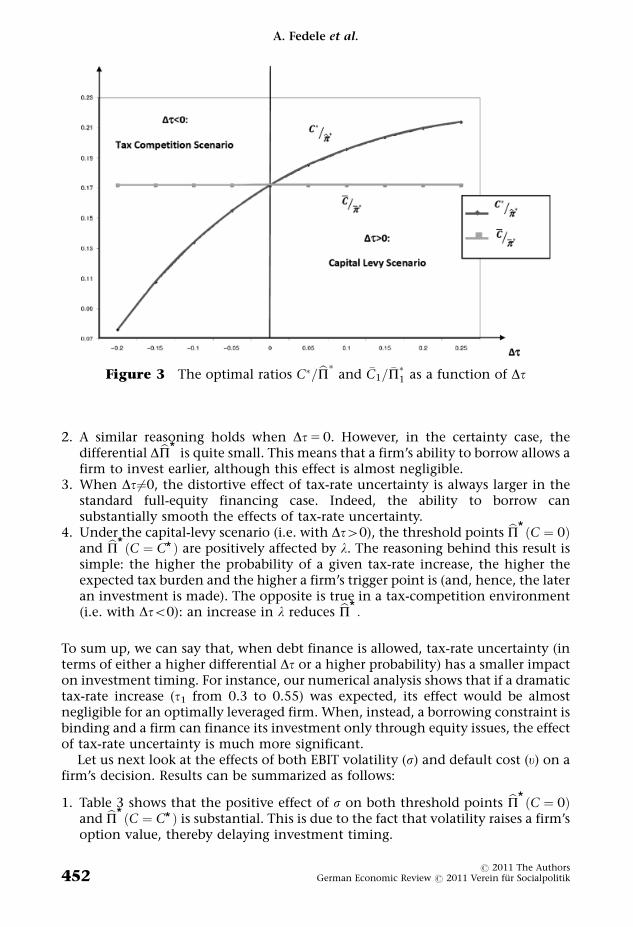
So far we have analyzed the absolute values of P and C. Let us next focus on thecoupon/EBIT ratio. In doing so, we will then compare the tax-rate-certainty ratio,

�C0= �P*0

� , with the tax-rate-uncertainty one, C*=bP*

� . As shown in Figure 3, ratio

C*=bP*�

is increasing in Dt (curved line); in other words, a firm’s propensity to

borrow increases with Dt. Of course, the ratio �C0= �P*0

� , depicted by the straight

line, is constant. It is worth noting that the curved line (tax-uncertainty case) isbelow (above) the straight line (tax-certainty case) if Dto0 (Dt40). This means thatwhen a tax rate is expected to decrease, the expected tax benefit of interestdeductibility will be lower and, therefore, debt will be less profitable than undertax-rate certainty. The converse is true if Dt40: in this case, a firm operating in anuncertain tax environment is stimulated to raise leverage.

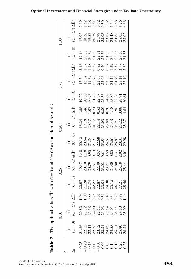
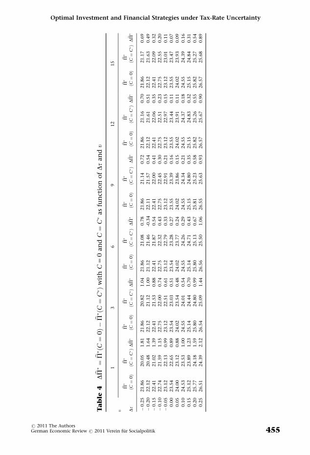
In Tables 2–4, we provide a sensitivity analysis for different values of Dt, l, s and u. Inorder to analyze how a firm’s ability to borrow affects its investment decisions, we willcompare the well-known full-equity finance case (C 5 0) with the optimal-leverage case(i.e. C ¼ C* ). Accordingly, we will calculate the threshold values under both full-equityfinancing (i.e. bP* C ¼ 0ð Þ) and optimal-leverage financing (i.e. bP* C ¼ C*ð Þ). Moreover,we will calculate the differential DbP* � bP* C ¼ 0ð Þ � bP* C ¼ C*ð Þ.

Table 1 The parameter values

Parameter Value

s 0.4I 100t0 0.3t1 [0.1, 0.55]r 0.05d 0.05u 3l [0.1, 1]

A. Fedele et al.


Let us first focus on the effects of tax-rate uncertainty (l) on a firm’s choice. Asshown in Table 2, we can see that:

1. For any given l, the inequality bP* C ¼ C*ð Þ< bP* C ¼ 0ð Þ holds. As expected,financial flexibility allows firms to invest earlier, in order to enjoy the tax benefitof interest deductibility.

Figure 2 (a) The optimal threshold points bP� and �P�1 as a function of Dt(b) The optimal coupons C� and �C1, debt levels D� and �D and their ratios as a function

of Dt



2. A similar reasoning holds when Dt5 0. However, in the certainty case, thedifferential DbP* is quite small. This means that a firm’s ability to borrow allows afirm to invest earlier, although this effect is almost negligible.

3. When Dt6¼0, the distortive effect of tax-rate uncertainty is always larger in thestandard full-equity financing case. Indeed, the ability to borrow cansubstantially smooth the effects of tax-rate uncertainty.

4. Under the capital-levy scenario (i.e. with Dt40), the threshold points bP* C ¼ 0ð Þand bP* C ¼ C*ð Þ are positively affected by l. The reasoning behind this result issimple: the higher the probability of a given tax-rate increase, the higher theexpected tax burden and the higher a firm’s trigger point is (and, hence, the lateran investment is made). The opposite is true in a tax-competition environment(i.e. with Dto0): an increase in l reduces bP* :

To sum up, we can say that, when debt finance is allowed, tax-rate uncertainty (interms of either a higher differential Dt or a higher probability) has a smaller impacton investment timing. For instance, our numerical analysis shows that if a dramatictax-rate increase (t1 from 0.3 to 0.55) was expected, its effect would be almostnegligible for an optimally leveraged firm. When, instead, a borrowing constraint isbinding and a firm can finance its investment only through equity issues, the effectof tax-rate uncertainty is much more significant.

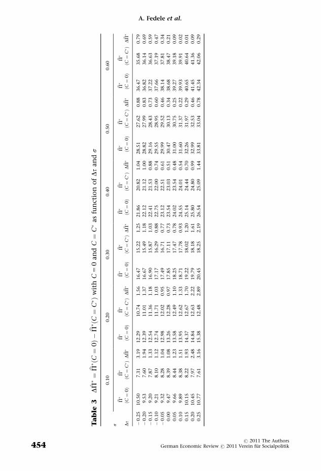
Let us next look at the effects of both EBIT volatility (s) and default cost (u) on afirm’s decision. Results can be summarized as follows:

1. Table 3 shows that the positive effect of s on both threshold points bP* C ¼ 0ð Þand bP* C ¼ C*ð Þ is substantial. This is due to the fact that volatility raises a firm’soption value, thereby delaying investment timing.

Figure 3 The optimal ratios C�=bP� and �C1= �P�1 as a function of Dt

A. Fedele et al.


Ta

ble

2T

he

op

tim

al

valu

esb P� w

ith

C5

0an

dC

5C

*as

fun

ctio

no

fDt

an

dl

l0.1

00.2

50.5

00.7

51.0

0

Dt

b P� ðC¼

0Þ

b P�ðC¼

C� Þ

Db P�

b P� ðC¼

0Þ

b P� ðC¼

C� ÞDb P�

b P� ðC¼

0Þ

b P� ðC¼

C� Þ

Db P�

b P� ðC¼

0Þ

b P� ðC¼

C� ÞDb P�

b P� ðC¼

0Þ

b P� ðC¼

C� Þ

Db P�

�0.2

521.8

620.8

21.0

420.8

719.4

71.4

020.1

218.2

41.8

819.7

217.5

42.1

819.4

617.0

72.3

9�

0.2

022.1

221.1

21.0

021.2

820.1

01.1

820.6

419.1

81.4

620.3

018.6

41.6

720.0

818.2

61.8

2�

0.1

522.4

121.5

30.8

821.7

420.7

90.9

521.2

420.1

71.0

720.9

719.7

91.1

820.7

919.5

21.2

8�

0.1

22.7

522.0

00.7

422.2

721.5

40.7

321.9

121.1

70.7

421.7

220.9

50.7

721.6

020.7

90.8

1�

0.0

523.1

222.5

10.6

122.8

722.3

00.5

722.6

822.1

40.5

322.5

722.0

50.5

222.5

121.9

90.5

20.0

023.5

423.0

30.5

123.5

423.0

30.5

123.5

423.0

30.5

023.5

323.0

30.5

023.5

323.0

30.5

00.0

524.0

223.5

40.4

824.3

023.7

10.5

924.5

123.8

00.7

024.6

223.8

50.7

724.6

923.8

70.8

20.1

24.5

524.0

10.5

425.1

524.3

00.8

525.6

124.4

31.1

825.8

624.4

71.3

926.0

224.4

81.5

40.1

525.1

424.4

40.7

026.1

124.8

01.3

126.8

724.9

11.9

627.2

724.9

02.3

727.5

424.8

62.6

80.2

025.8

024.8

00.9

927.2

125.1

82.0

228.3

125.2

23.0

828.9

125.1

43.7

729.3

025.0

34.2

60.2

526.5

425.0

91.4

428.4

625.4

43.0

129.9

825.3

74.6

130.8

125.1

95.6

231.3

525.0

26.3

3



Ta

ble

3DP�¼b P� ðC

¼0Þ�

b P� ðC¼

C� Þ

wit

hC

50

an

dC¼

C�

as

fun

ctio

no

fDt

an

ds

s

0.1

00.2

00.3

00.4

00.5

00.6

0

Dt

b P� ðC¼

0Þ

b P�ðC¼

C� Þ

Db P�

b P� ðC¼

0Þ

b P�ðC¼

C� Þ

Db P�

b P� ðC¼

0Þ

b P�ðC¼

C� Þ

Db P�

b P� ðC¼

0Þ

b P� ðC¼

C� Þ

Db P�

b P� ðC¼

0Þ

b P�ðC¼

C� Þ

Db P�

b P� ðC¼

0Þ

b P�ðC¼

C� Þ

Db P�

�0.2

510.5

07.3

13.1

912.2

910.7

41.5

616.4

715.2

21.2

521.8

620.8

21.0

428.5

127.6

20.8

836.4

735.6

80.7

9

�0.2

09.5

37.6

01.9

412.3

911.0

11.3

716.6

715.4

91.1

822.1

221.1

21.0

028.8

227.9

90.8

336.8

236.1

40.6

9

�0.1

59.2

07.8

71.3

312.5

411.3

61.1

816.9

015.8

71.0

322.4

121.5

30.8

829.1

628.4

30.7

337.2

236.6

30.5

9

�0.1

09.2

18.1

01.1

212.7

411.7

11.0

317.1

716.2

90.8

822.7

522.0

00.7

429.5

528.9

50.6

037.6

637.1

90.4

7

�0.0

59.3

28.2

81.0

412.9

812.0

20.9

517.4

916.7

10.7

723.1

222.5

10.6

129.9

929.5

20.4

638.1

437.8

10.3

4

0.0

09.4

78.3

91.0

813.2

612.2

80.9

717.8

517.1

10.7

323.5

423.0

30.5

130.4

730.1

30.3

438.6

838.4

70.2

1

0.0

59.6

68.4

41.2

313.5

812.4

91.1

018.2

517.4

70.7

824.0

223.5

40.4

831.0

030.7

50.2

539.2

739.1

80.0

9

0.1

09.8

98.3

81.5

113.9

512.6

21.3

318.7

117.7

80.9

324.5

524.0

10.5

431.6

031.3

70.2

239.9

339.9

10.0

2

0.1

510.1

58.2

21.9

314.3

712.6

71.7

019.2

218.0

21.2

025.1

424.4

40.7

032.2

631.9

70.2

940.6

540.6

40.0

1

0.2

010.4

57.9

72.4

814.8

412.6

32.2

219.7

918.1

81.6

125.8

024.8

00.9

932.9

932.5

30.4

641.4

541.3

60.0

9

0.2

510.7

77.6

13.1

615.3

812.4

82.8

920.4

518.2

52.1

926.5

425.0

91.4

433.8

133.0

40.7

842.3

442.0

60.2

9

A. Fedele et al.


Ta

ble

4Db P� ¼

b P� ðC¼

0Þ�

b P� ðC¼

C� Þ

wit

hC

50

an

dC¼

C�

as

fun

ctio

no

fDt

an

du

u

13

69

12

15

Dt

b P� ðC¼

0Þ

b P� ðC¼

C� Þ

Db P�

b P� ðC¼

0Þ

b P�ðC¼

C� Þ

Db P�

b P� ðC¼

0Þ

b P�ðC¼

C� Þ

Db P�

b P� ðC¼

0Þ

b P�ðC¼

C� Þ

Db P�

b P� ðC¼

0Þ

b P�ðC¼

C� Þ

Db P�

b P� ðC¼

0Þ

b P� ðC¼

C� Þ

Db P�

�0.2

521.8

620.0

51.8

121.8

620.8

21.0

421.8

621.0

80.7

821.8

621.1

40.7

221.8

621.1

60.7

021.8

621.1

70.6

9

�0.2

022.1

220.4

81.6

422.1

221.1

21.0

021.1

221.4

6-0

.34

22.1

121.5

70.5

422.1

221.6

10.5

122.1

221.6

30.4

9

�0.1

522.4

121.0

21.3

922.4

121.5

30.8

822.4

121.8

70.5

422.4

122.0

00.4

122.4

122.0

60.3

522.4

122.0

90.3

2

�0.1

022.7

421.5

91.1

522.7

522.0

00.7

422.7

522.3

20.4

322.7

522.4

50.3

022.7

522.5

10.2

322.7

522.5

50.2

0

�0.0

523.1

222.1

30.9

923.1

222.5

10.6

123.1

222.7

90.3

323.1

222.9

10.2

123.1

222.9

70.1

523.1

223.0

10.1

1

0.0

023.5

422.6

50.8

923.5

423.0

30.5

123.5

423.2

80.2

723.5

523.3

90.1

623.5

523.4

40.1

123.5

523.4

70.0

7

0.0

524.0

023.1

20.8

824.0

223.5

40.4

824.0

223.7

70.2

424.0

223.8

60.1

524.0

223.9

10.1

124.0

223.9

30.0

9

0.1

024.5

323.5

31.0

024.5

524.0

10.5

424.5

524.2

60.2

924.5

524.3

40.2

124.5

524.3

70.1

824.5

524.3

90.1

6

0.1

525.1

223.8

91.2

325.1

424.4

40.7

025.1

424.7

10.4

325.1

524.8

00.3

525.1

524.8

30.3

225.1

524.8

40.3

1

0.2

025.7

724.1

81.5

925.8

024.8

00.9

925.8

025.1

30.6

725.8

125.2

30.5

825.8

225.2

60.5

525.8

225.2

70.5

4

0.2

526.5

124.3

92.1

226.5

425.0

91.4

426.5

625.5

01.0

626.5

525.6

30.9

326.5

725.6

70.9

026.5

725.6

80.8

9



2. As shown in subsection 2.3.1., under tax-rate certainty (with t1), an increase in uraises the cost of default, and, therefore, discourages borrowing. Table 4 showsthat, under tax-rate uncertainty, the effect of u on both bP* C ¼ C*ð Þ andbP* C ¼ 0ð Þ is still positive, and, therefore, causes a delay in investment.

3. For any given couple (s,Dt) and (u,Dt), the differential DbP* is positive. Again, wecan see that financial flexibility allows firms to invest earlier in order to enjoythe tax benefit of interest deductibility.

4. For any given value of s and u, the value DbP* is U-shaped. This means that: (i) thedifferential DbP* is large when Dtj j is large, i.e. a firm’s ability to borrow allowsinvestment much earlier when a large variation of the tax rate is expected; (ii) thedifferential DbP* is minimum for Dt! 0. In this case, the effect of a firm’s abilityto borrow on investment timing is still positive, though it is relatively small.

4. A DISCUSSION OF THE RESULTS

All the relevant articles quoted in our introduction share the hypothesis of fullyequity financing. Apart from this common assumption, scholars have discusseddifferent cases where tax uncertainty may have an ambiguous effect on investmentdecisions. In particular, an ambiguity may arise if either investment tax credits areassumed to change unexpectedly (Hassett and Metcalf, 1999) or uncertainty affectsboth corporate and interest income taxation (Niemann, 2004; 2006). Analogously,the ability to accumulate capital gradually (see, e.g., Bohm and Funke, 2000) andthe existence of some monopolistic power (Bockem, 2001) may smooth or evenrevert the effects of tax uncertainty. Using an ACE-type system, Panteghini (2001a;2001b) has shown that tax-rate uncertainty does not affect one-off investment ifthe imputation rate is high enough. This result is an application of the well-knownbad news principle (see Bernanke, 1983), according to which if taxation affects onlygood events, it is neutral in terms of investment timing.

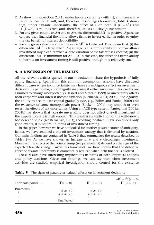
In this paper, however, we have not looked for another possible source of ambiguity.Rather, we have assumed a one-off investment strategy that is distorted by taxation.Our main findings are contained in Table 5 that summarizes the results described inTables 2–4. As we have shown, an increase in s and u discourages investment.Moreover, the effects of the Poisson jump (see parameter l) depend on the sign of theexpected tax-rate change. Given this framework, we have shown that the distortiveeffect of tax-rate uncertainty is dramatically reduced when debt finance is allowed.

These results have interesting implications in terms of both empirical analysisand policy decisions. Given our findings, we can say that when investmentactivities are studied, empirical investigation should control for the existence

Table 5 The signs of parameter values’ effects on investment decisions

Threshold points ! bP� C ¼ 0ð Þ bP� C ¼ C�ð ÞDbP� � bP� C ¼ 0ð Þ�bP� C ¼ C�ð Þ

Parameters #l

� if Dt< 0þ if Dt> 0

� if Dt< 0þ if Dt> 0

þs þ þ �u Unaffected þ �

A. Fedele et al.


(absence) of financial flexibility. Indeed, disregarding the characteristics of financialmarkets would be misleading.

Similarly, the effect of a hot policy debate on future (and uncertain) tax-ratechanges may have a significantly negative impact on investment, if firms are creditconstrained. If, however, financial markets are efficient and hence provide asufficient amount of resources, the same debate may lead to a negligible impact oninvestment, since firms can smooth the effects of tax-rate uncertainty by optimallyadjusting their capital structure. It is worth noting that we assumed the absence ofany renegotiation of debt. Of course we expect that, whenever renegotiation isallowed, a firm enjoys a higher degree of flexibility and the effect of tax-rateuncertainty is further mitigated.

5. CONCLUSION

In this article, we have applied a real-option model to study the effects of tax-rateuncertainty on both investment timing and the optimal capital structure of arepresentative firm.

By departing from the relevant literature, which has extensively analyzed fullyequity-financed investment decisions, we have shown that the ability to borrowallows firms to invest earlier in order to enjoy the tax benefit of interestdeductibility. More importantly, we have shown that a highly volatile tax systemmay have a negligible impact on investment choices, when firms can choose theircapital structure. This leads us to conclude that debt finance allows a firm tosmooth substantially the distortive effects of tax-rate uncertainty.

In this paper we have used some simplifying assumptions, such as the symmetrictreatment of profits and losses, as well as the absence of personal taxation, agencycosts and any bargaining process between stakeholders (including renegotiationand partial conversion of debt into equity). The elimination of any of thesesimplifying assumptions is an interesting topic that we leave for future research.Finally, evidence shows that tax uncertainty is caused by both tax-rate and tax-basechanges (e.g. via changes in investment tax credits and fiscal depreciationallowances), as well as by unexpected changes in the treatment of interest income.Therefore, a promising extension of our model would entail the joint analysis ofsources of uncertainty.

APPENDIX A: THE VALUE FUNCTIONS

In order to calculate a firm’s value function with tax-rate uncertainty, we must firstfocus on the value function after the tax-rate change, i.e. when tax rate is t1.Subsequently, we will deal with the value function under tax-rate uncertainty, i.e.when the current tax rate is t0.

A.1. The value function (4)

Using dynamic programming, let us calculate the predefault equity value E1(P; C)as a summation between the net cash flow (1� t1)(P�C), in the short interval dt,and its future value after the instant dt has passed

E1 P; Cð Þ ¼ 1� t1ð Þ P� Cð Þdt

þ e�rdtx E1 Pþ dP; Cð Þ½ �; with P>C ðA1Þ



where x[E1(Pþ dP; C)] is the expected value of equity at time tþ dt. Expanding theright-hand side of (A1), applying Ito’s lemma and rearranging gives the followingnon-arbitrage condition

rE1 P; Cð Þ ¼ 1� t1ð Þ P� Cð Þ þ ðr � dÞPE1P P; Cð Þ

þ s2

2P2E1PP P; Cð Þ ðA2Þ

where d � r� a, E1P � ›E=›P and E1PP � ›2E=›2P.Note that, when default takes place (i.e. when P goes to C), shareholders are

expropriated, and, therefore, the value of their claim is nil, i.e. E1(C; C) 5 0.Accordingly, the general-form solution of (A2) is

E1 P; Cð Þ ¼0 after default

1� t1ð Þ Pd � C

r

� �þP2i¼1

AiPbi before default

8<: ðA3Þ

where b1 ¼ ð1=2Þ � ððr � dÞ=s2Þ þffiffiffiffiffiffiffiffiffiffiffiffiffiffiffiffiffiffiffiffiffiffiffiffiffiffiffiffiffiffiffiffiffiffiffiffiffiffiffiffiffiffiffiffiffiffiffiffiffiffiffiffiffiffiffiffiffiffiffiffiffiffiffiffiffiffiffiffiððr � dÞ=s2Þ � ð1=2Þð Þ2 þ ð2r=s2

qÞ> 1 and b2 ¼

ð1=2Þ � ððr � dÞ=s2Þ �ffiffiffiffiffiffiffiffiffiffiffiffiffiffiffiffiffiffiffiffiffiffiffiffiffiffiffiffiffiffiffiffiffiffiffiffiffiffiffiffiffiffiffiffiffiffiffiffiffiffiffiffiffiffiffiffiffiffiffiffiffiffiffiffiffiffiffiffiððr � dÞ=s2Þ � ð1=2Þð Þ2 þ ð2r=s2

qÞ< 0 are the roots of the

characteristic equation CðbÞ ¼ ð1=2Þs2bðb� 1Þ þ ðr � dÞb� r ¼ 0.Let us next calculate A1 and A2. In the absence of any financial bubbles, A1 is nil.

To calculate A2, we must consider that default occurs when P drops to C, namelythe condition

E1 C; Cð Þ ¼ 1� t1ð Þ C

d� C

r

� �þ A2Cb2 ¼ 0

holds. Rearranging this equation gives

A2 ¼ � 1� t1ð Þ C

d� C

r

� �� C�b2

Using these results, we can therefore rewrite (A3) as

E1 P; Cð Þ ¼0 after default1� t1ð Þ P

d � Cr

� �� C

d � Cr

� �PC

� �b2

h ibefore default

�ðA4Þ

Following the same procedure let us next write the predefault value of debt as

D1 P; Cð Þ ¼ Cþ e�rdtx D1 Pþ dP; Cð Þ½ � ðA5Þ

When default takes place and the firm is expropriated, the lender’s claim is givenby the firm’s value and is therefore equal to

D1 P; Cð Þ ¼ 1� t1ð ÞPþ e�rdtx D1 Pþ dP; Cð Þ½ � ðA6Þ

A. Fedele et al.


Expanding the right-hand side, applying Ito’s lemma and rearranging (A5) and(A6) gives the following non-arbitrage condition:

rD1 P; Cð Þ ¼ 1� t1ð ÞPþ ðr � dÞPD1PðP; CÞ þ s2

2 P2D1PPðP; CÞ after default

Cþ ðr � dÞPD1PðP; CÞ þ s2

2 P2D1PPðP; CÞ before default

(ðA7Þ

The closed-form solution of (A7) is

D1 P; Cð Þ ¼

1�t1ð ÞPd þ

P2i¼1

BiPbi after default

Cr þ

P2i¼1

DiPbi before default

8>>><>>>: ðA8Þ

To calculate B2 we use the boundary condition D(0; C) 5 0 which means thatwhen P falls to zero the lender’s postdefault claim is nil. This implies that B2 5 0. Inthe absence of any financial bubble, we have B1 5 D1 5 0. Finally, to calculate D2 welet the predefault branch of (A8) equate its after-default one, net of the default costuC, at point P5 C. We thus obtain

C

rþD2Cb2 ¼ 1� tð ÞC

d� uC ðA9Þ

Solving (A9) for D2 yields D2 ¼ ðð 1� t1ð ÞCÞ=dÞ � ðC=rÞ � uC½ �C�b2 , and hence,(A8) reduces to

D1 P; Cð Þ ¼1�t1ð ÞP

d after default1r þ

1�t1

d � 1r � u

� �PC

� �b2

h iC before default

(ðA10Þ

The summation of (A4) and (A10), net of the investment cost I, yields

V1ðP; CÞ ¼ E1 P; Cð Þ þD1 P; Cð Þ � I

¼ 1� t1ð ÞPd

þ t1C

r� t1

rþ u

� C

PC

� �b2

� I ðA11Þ

A.2. The value function (5)

Following the same procedure we can calculate the value function before the tax-rate change. Again, we write the predefault value of equity as

E0 P; Cð Þ ¼ 1� t0ð Þ P� Cð Þ

þ 1� ldtð Þe�rdtx E0 Pþ dP; Cð Þ½ �

þ ldte�rdtx E1 Pþ dP; Cð Þ½ �

As can be seen, E0(P; C) is equal to (1� t0)(P�C) plus the weighted average offunctions x[E0(Pþ dP; C)] and x[E1(Pþ dP; C)], where the weights are given by theprobability that the tax-rate change may or may not occur in the interval dt. The



probability that the change does not occur during the period dt is equal to (1� ldt),while the probability that this event takes place is equal to ldt. Multiplying theseprobabilities by the expected values at time tþ dt (i.e. by e�rdt x[E0(Pþ dP; C)]when the tax-rate change does not occur and by e�rdt x[E1(Pþ dP; C)] when thechange occurs, respectively) and adding (1� t0)(P�C) thus gives E0(P; C).24

Expanding its right-hand side, applying Ito’s lemma and rearranging gives

r þ lð ÞE0 P; Cð Þ ¼ 1� t0ð Þ P� Cð Þ þ ðr � dÞPE0P P; Cð Þ

þ s2

2P2E0PP P; Cð Þ þ lE1 P; Cð Þ ðA12Þ

Let us next subtract (A2) from (A12) so that

r þ lð ÞX P; Cð Þ ¼ t1 � t0ð Þ P� Cð Þ þ ðr � dÞPXP P; Cð Þ

þ s2

2P2XP P; Cð Þ ðA13Þ

where

X P; Cð Þ � E0 P; Cð Þ � E1 P; Cð Þ ðA14Þ

Solving (A13) yields

X P; Cð Þ ¼ t1 � t0ð Þ Pdþ l

� C

r þ l

� �þX2

i¼1

FiPbi lð Þ ðA15Þ

where

b1 lð Þ ¼ 1

2� r � d

s2þ

ffiffiffiffiffiffiffiffiffiffiffiffiffiffiffiffiffiffiffiffiffiffiffiffiffiffiffiffiffiffiffiffiffiffiffiffiffiffiffiffiffiffiffiffiffiffiffiffiffiffiffir � ds2� 1

2

� �2

þ 2 r þ lð Þs2

s> 1

b2 lð Þ ¼ 1

2� r � d

s2�

ffiffiffiffiffiffiffiffiffiffiffiffiffiffiffiffiffiffiffiffiffiffiffiffiffiffiffiffiffiffiffiffiffiffiffiffiffiffiffiffiffiffiffiffiffiffiffiffiffiffiffir � ds2� 1

2

� �2

þ 2 r þ lð Þs2

s< 0

are the roots of the characteristic equation

CðbÞ ¼ 1

2s2bðb� 1Þ þ ðr � dÞb� r þ lð Þ ¼ 0

Note that, in the absence of bubbles, we have F1 5 0. Using (A14) and (A15), andrearranging, we obtain

E0 P; Cð Þ ¼ E1 P; Cð Þ þ X P; Cð Þ ¼ 1� t1ð Þ Pd� C

r

� �� C

d� C

r

� �PC

� �b2

" #

þ t1 � t0ð Þ Pdþ l

� C

r þ l

� �þ F2Pb2 lð Þ ðA16Þ

24. For further details, see Dixit and Pindyck (1994, p. 203).

A. Fedele et al.


If default occurs, the value of equity goes to zero, i.e. E0(C; C) 5 0. Using thisdefault condition and solving (A16) for F2 we can find

F2 ¼ � t1 � t0ð Þ C

dþ l� C

r þ l

� �C�b2 lð Þ

Hence, the value of equity is equal to

E0 P; Cð Þ ¼ E1 P; Cð Þ þ X P; Cð Þ ¼ 1� t1ð Þ Pd� C

r

� �� C

d� C

r

� �PC

� �b2

" #


� C

r þ l

� ��

� C

dþ l� C

r þ l

� �PC

� �b2 lð Þ#

ðA17Þ

Let us now calculate the value of debt before the tax-rate change. As usual, wecan write it as

D0 P; Cð Þ ¼ K þ 1� ldtð Þe�rdtx D0 Pþ dP; Cð Þ½ �

þ ldte�rdtx D1 Pþ dP; Cð Þ½ � ðA18Þ

where K 5 C and K 5 (1� t0)P are the flow before and after default, respectively.Expanding the right-hand side of (A18), applying Ito’s lemma and rearranging givesthe following non-arbitrage condition

r þ lð ÞD0 P; Cð Þ ¼ K þ r � dð ÞPD0P P; Cð Þ

þ s2

2P2D0PP P; Cð Þ þ lD1 P; Cð Þ ðA19Þ

Subtracting (A7) from (A19) and defining

Y P; Cð Þ � D0 P; Cð Þ �D1 P; Cð Þ ðA20Þ

yields

r þ lð ÞY P; Cð Þ ¼ J þ r � dð ÞPYP P; Cð Þ

þ s2

2P2YPP P; Cð Þ ðA21Þ

where J 5 0 and J 5 (t1� t0)P are the relevant flows before and after default,respectively. The solution of (A21) has the following form

YðP; CÞ ¼

ðt1�t0ÞPdþl þ

P2i¼1

LiPbiðlÞ after default

P2i¼1

GiPbiðlÞ before default

8>>><>>>:



Note that, after default (but before the tax-rate change), the boundary conditionY(0; C) 5 0 holds. This implies that L2 5 0. Moreover, in the absence of bubbles, wehave L1 5 G1 5 0.

Remember that, after default, the lender becomes a shareholder. Therefore, using(A21) and rearranging, we can write the firm’s value after default

D0 P; Cð Þ ¼ 1� t1ð Þd

þ t1 � t0ð Þdþ l

� �P

Following the same procedure we can write the before-default value of debt

D0 P; Cð Þ ¼ 1

rþ 1� t1ð Þ

d� 1

r� u

� �PC

� �b2

( )Cþ G2Pb2 lð Þ ðA22Þ

To find G2 we let the two branches of the debt function meet at point P5 C andaccount for the default cost. This means that the equality

1� t1

dCþG2Cb2 lð Þ ¼ 1� t1

dþ t1 � t0

dþ l

� �C� uC ðA23Þ

holds. Solving (A23) for G2 and substituting the result into (A22) yields

D0 P; Cð Þ ¼ 1

rþ 1� t1

d� 1

r� u

� �PC

� �b2

" #C

þ t1 � t0

dþ lC

PC

� �b2 lð ÞðA24Þ

Using (A17) and (A24), we can finally calculate the firm’s NPV

V0 P; Cð Þ ¼ 1� t1ð Þ Pd� C

r

� �� C

d� C

r

� �PC

� �b2

" #þ


� C

r þ l

� ��

� C

dþ l� C

r þ l

� �PC

� �b2 lð Þ#

þ 1

rþ 1� t1

d� 1

r� u

� �PC

� �b2

" #C

þ t1 � t0

dþ lC

PC

� �b2 lð Þ� I ðA25Þ

A. Fedele et al.


APPENDIX B: THE OPTION FUNCTIONS

B.1. The option function (9)

Using dynamic programming we can write a firm’s option to invest under tax-ratecertainty as

O1 P; Cð Þ ¼ e�rdtx O1 Pþ dP; Cð Þ½ �

Expanding its right-hand side, applying Ito’s lemma and rearranging gives thefollowing non-arbitrage condition

rO1 P; Cð Þ ¼ r � dð ÞPO1P P; Cð Þ þ s2

2P2O1P P; Cð Þ ðB1Þ

Solving (B1) gives the following general closed-form solution

O1 P; Cð Þ ¼X2

j¼1

HjPbj ðB2Þ

When P goes to zero, in a geometric Brownian motion it will remain zero. Thisimplies that H2 5 0 (see Dixit and Pindyck, 1994), and therefore (B2) reduces to (6).

B.2. The option function (10)

Let us next calculate the firm’s option to invest O0(P; C) under tax-rate uncertainty.Function O0(P; C) is equal to the weighted average of functions x[O0(Pþ dP; C)]and x[O1(Pþ dP; C)], where the weights are given by the probability that the tax-rate change may or may not occur in the interval dt. Multiplying these probabilitiesby the values at time tþ dt (i.e. by e� rdt x[O0(Pþ dP; C)] when the tax-rate changedoes not occur and by e� rdt x[O1(Pþ dP; C)] when the change occurs, respectively)gives

O0 P; Cð Þ ¼ 1� ldtð Þe�rdtx O0 Pþ dP; Cð Þ½ �

þ ldte�rdtx O1 Pþ dP; Cð Þ½ �

Expanding its right-hand side, applying Ito’s lemma and rearranging gives thefollowing non-arbitrage condition

r þ lð ÞO0 P; Cð Þ ¼ r � dð ÞPO0PP P; Cð Þ

þ s2

2P2O0PP P; Cð Þ þ lO1 P; Cð Þ ðB3Þ

Subtracting (B1) from (B3) gives

r þ lð ÞZ P; Cð Þ ¼ r � dð ÞPZP P; Cð Þ

þ s2

2P2ZPP P; Cð Þ ðB4Þ



where Z(P; C) � O0(P; C)�O1(P; C). Solving (B4), we have

Z P; Cð Þ ¼X2

i¼1

ZiPbi lð Þ

Since Z(0; C) 5 0, we obtain

Z P; Cð Þ ¼ Z1Pb1 lð Þ

and therefore, the option value can be rewritten as

O0 P; Cð Þ ¼ O1 P; Cð Þ þ Z P; Cð Þ

¼ H1Pb1 þ Z1Pb1 lð Þ ðB5Þ

To calculate Z1 we apply the VMC at the threshold point P ¼ bPV0ðP; CÞj

P¼bP ¼ O0 P; Cð ÞjP¼bP ðB6Þ

Using (B5) and (B6), we obtain

H1bPb1 þ Z1

bPb1 lð Þ ¼ V0bP; C�

ðB7Þ

which gives

Z1 ¼ V0bP; C�

�H1bPb1

h ibP�b1 lð Þ

and therefore

Z1Pb1 lð Þ ¼ V0bP; C�

�H1bPb1

h i PbP� �b1 lð Þ

ðB8Þ

Substituting (B8) into (B7), using (B6) and rearranging gives (10).

APPENDIX C: THE FIRM’S CHOICE UNDER TAX-RATE CERTAINTY

Under tax-rate certainty, the firm’s problem is (13).

C.1. The solutions

The first-order conditions of (13) with respect to C and �P are

P�P

� �b1 1

rt1 � 1� b2ð Þ t1 þ urð Þ

�PC

� �b2

" #¼ 0 ðC1Þ

P�P

� �b1 1�P

1� t1ð Þ �Pr

� b2

C

rt1 þ urð Þ

�PC

� �b2

þ(

�b1

1� t1ð Þ �Pr

þ C

rt1 � t1 þ urð Þ

�PC

� �b2

!� I

" #)¼ 0 ðC2Þ

A. Fedele et al.


respectively. Rearranging (C1) gives

C ¼ 1

1� b2

t1

t1 þ ru

� �� 1b2 �P ðC3Þ

Moreover, from (C1) we obtain

t1

1� b2

¼ t1 þ urð Þ�PC

� �b2

and hence, we can rewrite (C2) as

1� t1ð Þ �Pr

� b2

C

r

t1

1� b2

� �

� b1

1� t1ð Þ �Pr

þ C

rt1 �

t1

1� b2

� �� I

� �¼ 0 ðC4Þ

Rearranging and dividing (C4) by ½ 1� b1ð Þ 1� t1ð Þ�=r one obtains

�Pþ t1

1� t1

b2

b2 � 1C� b1

b1 � 1

r

1� t1I ¼ 0 ðC5Þ

Substituting (C3) into (C5) gives

�P*1 ¼

1

1þm1

b1

b1 � 1

r

1� t1I

where m1 � ðt1=ð1� t1ÞÞðb2=ðb2 � 1ÞÞ ð1=ð1� b2ÞÞðt1=ðt1 þ urÞÞ½ ��1b2 > 0. The second-

order condition with respect to C is verified. Indeed

›2O1

›C2¼ P

�P

� �b1 t1 þ rur

1� b2ð Þb2

�PC

� �b2�1

�PC�2

Rearranging

P�P

� �b1 t1 þ rur

1� b2ð Þb2C�1�PC

� �b2

Since b2o0, derivative ›2O1=›C2 is always negative. Solution (14) is thusobtained.



C.2. Comparative statics

Let us next provide some comparative statics for �P*1 ;

�C1 and m1. Their derivativeswith respect to t1 are

› �P*1

›t1¼ b1

b1 � 1

rI

1� t1ð Þ21þm1 � ›m1

›t11� t1ð Þ

1þm1ð Þ2;

› �C1

›t1¼ 1� b2ð Þ t1 þ ruð Þ

t1

� � 1b2 › �P*

1

›t1� 1

b2t1

rut1 þ ru

�P*1

!;

›m1

›t1¼ b2

b2 � 1

1

1� b2

� �� 1b2

1þ urt1

� � 1b2

t1 þ urð Þb2 � ur 1� t1ð Þ1� t1ð Þ2b2 t1 þ urð Þ

> 0 ðC6Þ

It is easy to verify that ð›m1=›t1Þ< ð1þm1Þ=ð1� t1Þ, hence, we can state that› �P*

1=›t1 > 0. Given this result, we see that › �C1=›t1 > 0 and

›�C1

�P*1

� �›t1

¼ � 1

1� b2

� �� 1b2 1

b2

t1

t1 þ ru

� ��1�b2

b2 ru

t1 þ ruð Þ2> 0:

ACKNOWLEDGEMENTS

We would like to thank two anonymous reviewers, Hamed Ghoddusi and theseminar audience at the 10th Venice Summer Institute Workshop on ‘Operatinguncertainty using real options’, Venice International University, San Servolo, 8–9July 2009 for their useful comments. The usual disclaimer applies.

Addresses for correspondence: Alessandro Fedele, Department of Economics,University of Brescia, Via S. Faustino 74/B, 25122, Brescia, Italy. Tel.: þ 39 030 2988827; fax: þ 39 030 298 8837; e-mail: [email protected]

REFERENCES

Agliardi, E. (2001), ‘Taxation and Investment Decisions – A Real Option Approach’,Australian Economic Papers 40, 44–55.

Alvarez, L. H. R., V. Kanniainen and J. Sodersten (1998), ‘Tax Policy Uncertainty andCorporate Investment: A Theory of Tax-Induced Investment Spurts’, Journal of PublicEconomics 69, 17–48.

Amaro de Matos, J. (2001), Theoretical Foundations of Corporate Finance, Princeton UniversityPress, Princeton.

Bernanke, B. S. (1983), ‘Irreversibility, Uncertainty, and Cyclical Investment’, QuarterlyJournal of Economics 98, 85–103.

Bockem, S. (2001), ‘Investment and Politics – Does Tax Fear Delay Investment?’, FinanzArchiv58, 60–77.

Bohm, H. and M. Funke (2000), ‘Optimal Investment Strategies under Demand and TaxPolicy Uncertainty’, CESifo Working Paper No. 311.

A. Fedele et al.


mailto:[email protected]

Branch, B. (2002), ‘The Costs of Bankruptcy: A Review’, International Review of FinancialAnalysis 11, 39–57.

Brennan, M. J. and E. S. Schwartz (1977), ‘Convertible Bonds: Valuation and OptimalStrategies for Call and Conversion’, Journal of Finance 32, 1699–1715.

Chen, Y.-F. and M. Funke (2008), ‘Political Risk, Economic Integration, and the Foreign DirectInvestment Decision’, Dundee Discussion Papers in Economics No. 208.

Devereux, M. P., B. Lockwood and M. Redoano (2008), ‘Do Countries Compete overCorporate Tax Rates?’, Journal of Public Economics 92, 1210–1235.

Dixit, A. K. and R. S. Pindyck (1994), Investment under Uncertainty, Princeton University Press,Princeton.

Dixit, A. K. and R. S. Pindyck (1999), ‘Expandability, Reversibility, and Optimal CapacityChoice’, in: M. J. Brennan and L. Trigeorgis (eds.), Project Flexibility, Agency, andCompetition, Oxford University Press, Oxford, pp. 50–70.

Eichengreen, B. (1990), ‘The Capital Levy in Theory and Practice’, in: R. Dornbusch and M.Draghi (eds.), Public Debt Management: Theory and History, Cambridge University Press,Cambridge, pp. 191–220.

Ghinamo, M., P. M. Panteghini and F. Revelli (2010), ‘FDI Determination and CorporateTax Competition in a Volatile World’, International Tax and Public Finance 17, 532–555.

Goldstein, R., N. Ju and H. Leland (2001), ‘An EBIT-Based Model of Dynamic CapitalStructure’, Journal of Business 74, 483–512.

Graham, J. R. and C. R. Harvey (2001), ‘The Theory and Practice of Corporate Finance:Evidence from the Field’, Journal of Financial Economics 60, 187–243.

Hassett, K. A. and G. E. Metcalf (1999), ‘Investment with Uncertain Tax Policy: Does RandomTax Policy Discourage Investment?’, Economic Journal 109, 372–393.

Hennessy, C. and T. M. Whited (2005), ‘Debt Dynamics’, Journal of Finance 60, 1129–1165.KPMG (2009), Corporate and Indirect Tax Rate Survey 2008.Jensen, M. C. and W. Meckling (1976), ‘Theory of the Firm: Managerial Behavior, Agency

Costs, and Ownership Structure’, Journal of Financial Economics 7, 305–360.Leland, H. E. (1994), ‘Corporate Debt Value, Bond Covenants, and Optimal Capital

Structure’, Journal of Finance 49, 1213–1252.Leland, H. E. (1998), ‘Agency Costs, Risk Management, and Capital Structure’, Journal of

Finance 53, 1213–1243.Mauer, D. C. and S. H. Ott (2000), ‘Agency Costs, Underinvestment, and Optimal Capital

Structure’, in: M. J. Brennan and L. Trigeorgis (eds.), Perfect Flexibility, Agency, andCompetition, New Developments in the Theory and Application of Real Options, OxfordUniversity Press, New York.

Mauer, D. C. and S. Sarkar (2005), ‘Real Options, Agency Conflicts, and the Optimal CapitalStructure’, Journal of Banking and Finance 29, 1405–1428.

Miller, M. H. (1977), ‘Debt and Taxes’, Journal of Finance 32, 261–275.Mintz, J. M. (1995), ‘The Corporation Tax: A Survey’, Fiscal Studies 16, 23–68.Modigliani, F. and M. H. Miller (1958), ‘The Cost of Capital, Corporation Finance, and the

Theory of Investment’, American Economic Review 48, 261–297.Modigliani, F. and M. H. Miller (1963), ‘Corporate Income Taxes and the Cost of Capital: A

Correction’, American Economic Review 53, 433–443.Myers, S. C. (1977), ‘Determinants of Corporate Borrowing’, Journal of Financial Economics 3,

799–819.Niemann, R. (1999), ‘Neutral Taxation under Uncertainty – a Real Options Approach’,

FinanzArchiv 56, 51–66.Niemann, R. (2004), ‘Tax Rate Uncertainty, Investment Decisions, and Tax Neutrality’,

International Tax and Public Finance 11, 265–281.Niemann, R. (2006), ‘The Impact of Tax Uncertainty on Irreversible Investment’, arqus

Diskussionsbeitrag Nr. 21.



Niemann, R. and C. Sureth (2004), ‘Tax Neutrality under Irreversibility and Risk Aversion’,Economics Letters 84, 43–47.

Niemann, R. and C. Sureth (2005), ‘Capital Budgeting with Taxes under Uncertainty andIrreversibility’, Jahrbucher fur Nationalokonomie und Statistik 225, 77–95.

Panteghini, P. M. (2001a), ‘On Corporate Tax Asymmetries and Neutrality’, German EconomicReview 2, 269–286.

Panteghini, P. M. (2001b), ‘Corporate Tax Asymmetries under Investment Irreversibility’,FinanzArchiv 58, 207–226.

Panteghini, P. M. (2007a), Corporate Taxation in a Dynamic World, Springer, Berlin.Panteghini, P. M. (2007b), ‘Interest Deductibility Under Default Risk and the Unfavorable Tax

Treatment of Investment Costs: A Simple Explanation’, Economics Letters 96, 1–7.Pindyck, R. S. (2007), ‘Mandatory Unbundling and Irreversible Investment in Telecom

Networks’, Review of Network Economics 6, 274–298.Smith, C. W. Jr and J. B. Warner (1979), ‘On Financial Contracting: An Analysis of Bond

Covenants’, Journal of Financial Economics 7, 117–161.Sureth, C. (2002), ‘Partially Irreversible Investment Decisions and Taxation under

Uncertainty: A Real Option Approach’, German Economic Review 3, 185–221.

A. Fedele et al.


optimal investment and financial strategies under tax-rate uncertainty

Documents