NASA Contractor Report 17751 5

Optimal Guidance with LB Obstacle Avoidance

for Nap-of-the-Earth Flight ra

Nicholas J. Pekelsma

[SASB-a- 17753 5 ) DP"SIf%_tBt; GUf D&NCE 8PTH %89 -2 h13 28 QBSTgCSB BVOIDIHCE FOB HAP-OP9BE-EHPWT 8 G [Tan C O W * ) , 72 a C S C L O l C

tinclass 63/08 8217934

h CONTRACT NAS2-12402 December 1988

National Aeronautics and Space Administration

https://ntrs.nasa.gov/search.jsp?R=19890014957 2018-06-25T04:42:32+00:00Z

NASA Contractor Report 17751 5

Optimal Guidance with Obstacle Avoidance

d

for Nap-of-the-Earth Flight 1

Nicholas J. Pekelsma

Tau Corporation, LosGatos, California

Prepared for Ames Research Center CONTRACT NAS2-12402 December 1988

National Aeronautics and Space Administration

Ames Research Center Moffett Field, California 94035

TABLE OF CONTENTS

1.1 INTRODUCTION 1.2 RESEARCH OBJECTIVE 1.3 REPORT ORGANIZATION

2.0 FAR FIELD NAVIGATION - THE DYNAPLAN MISSION PLANNING WORKSTATION 5

2.1 GOAL 2.1.1 Initial Objectives 2.1.2 Current Codiguration of the Far Field Mission Planning Workstation

2.2 DYNAPLAN SOFTWARE 2.2.1 DMA Map and Cost Grid Handling 2.2.2 Threat Masking 2.2.3 Commanded Waypoints and Route Optimization 2.2.4 Data Management 2.2.5 Map Management

3.0 NEAR FIELD NAVIGATION - THE DYNAPATH SOFIWARE 22

3.1 INTRODUCllON 3.2 OVERVIEW OF DYNAPATH TF/TA OPTIMIZATION 3.3 THE DYNAPATEI TF/TA/NOE ALGORITHM 3.4 DYNAPATH ALGORITHM DEVELOPMENT

3.4.1 Core Algorithm Developments 3.4.2 Interface Algorithms

3.5 KEY PARAMETERS WHICH AFFECT THE SOLUTION PROCESS 3.6 ENHANCEMENTS NEEDED FOR DYNAPATH FLIGHT TESTING

4.0 DMA DIGITAL MAP INTERFACE 59

5.0 CONCLUSION 64

REFERENCES 65

LIST OF FIGURES

Figure 1 - 1 Relationship of Mission Planning and Terrain Following/ Terrain Avoidance/Threat Avoidance 1

Figure 1-2 System Interfaces for an Automated NOE Helicopter 2 Figure 1-3 Navigation and Guidance Domains for TF/TA Flight 3 Figure 2- 1 TAU Mission Planning and Image Exploitation Workstation 6 Figure 2-2 Threat Data List 10 Figure 2-3 Sample Missile Data Displayed by Dynaplan 10 Figure 2-4 Terrain Masking of Threat 11 Figure 2-5 Commanded Waypoints 11 Figure 2-6 Optimization Through Commanded Waypoints 13 Figure 2-7 Optimization with Enroute Targets 13 Figure 2-8 Route Opthnbation in the Presence of Several Threats 14 Figure 2-9 Alternate Route Through Commanded Waypoints 14 Figure 2- 10 Sample Flight Log 16 Figure 2- 1 1 Terrain Elevation Profile 16 Figure 2- 12 Interactive Cost Adjustment Module 17 Figure 2- 13 Removal of Terrain Avoidance as an Optimization Measure 17 Figure 2- 14 Automatic Route Smoothing 19 Figure 2- 15 Sample Dynapath Corridors 19 Figure 2- 16 Translation of Screen Coordinates to Earth Angles 2 1 Figure 3- 1 Patch Computation Performance Measure 24 Figure 3-2 Block Diagram of Dynapath Interfaces 25 Figure 3-3 Vertical Solution Procedure 26 Figure 3-4 Dynamic Programming Overlay 29 Figure 3-5 Dynapath Process Flow 3 1 Figure 3-6 Number of Computations 33 Figure 3-7 Refined Vertical Path Determination 3 5 Figure 3-8 Dynamic Programming Grid for Tuming At Waypoints 36 Figure 3-9 Sample Lateral Paths Over a Patch 38 Figure 3- 10 Sample DP Patch with a Deadband 38 Figure 3- 1 1 Dynapath Main Menu 40 Figure 3-12 Route Segment Menu 4 1 Figure 3- 13 Waypoint Menu 4 1 Figure 3- 14 Threat Menu 41 Figure 3- 15 NASA NOE Terrain Database Waypoint Set #6 44 Figure 3-16 Performance Analysis Cost vs CPU NASA NOE Database Waypoint Set #6 45 Figure 3-17 Performance Analysis Cost vs CPU NASA NOE Database Waypoint Set #6 46 Figure 3- 18 Dynapath Performance 48 Figure 3- 19 Dynapath Performance Summary 48 Figure 3-20 Dynapath Dual Step Performance 50 Figure 3-2 1 Patch Length Compute Time Sensitivity 5 1 Figure 3-22 Block Diagram of Dynapath Interfaces in a Real-Time Environment 52 Figure 3-23 Dynapath Capture Geometry 53 Figure 3-24 Dynapath Route Segment Geometry 5 5 Figure 3-25 Level Flight Power Required at SL/STD 57

LIST OF FIGURES (continued)

Figure 4- 1 Compressed Digital Map San Francisco (North) Figure 4-2 Dynapath Trajectory Rounding the Angel Island Waypoint Figure 4-3 Choices of Dynapath Trajectories through San Francisco Figure 4-4 Dynapath Trajectory NOE Flight Starting in Marin County Figure 4-5 Dynapath NOE Trajectory in Mountainous Terrain Figure 4-6 Rounding a Waypoint in Mountainous Terrain

ABBREVIATIONS

AAA Anti-Aircraft Artillery AGL Above Ground Level CGI Computer Graphics Interface DFAD Digital Feature Analysis Data DLMS Digital Land Mass DMA Defense Mapping Agency DP Dynamic Programming DTED Digital Terrain Elevation Data FLIR Forward-Looking Infrared GN&C Guidance Navigation and Control GPS Global Positioning System HACK Helicopter Air Combat Terrain Database HDD Head Down Display HGC Horizontal Command Generator HUD Head Up Display ICAB NASA's Fixed Base Real-Time Simulator IMINT Imagery Intelligence INS Inertial Navigation System LAN Local Area Network LI-IX Light Helicopter Experimental NOE Nap-of-the-Earth OA Obstacle Avoidance SAM Surface-to-Air Missile SBIR Small Business Innovative Research TF/TA Terrain Following/Terrain Avoidance VGC Vertical Command Generator USGS United States Geological Survey

1.1 INTRODUCTION

This Final SBIR Phase I1 Technical Report documents the results of work performed for the NASA-Ames Research Center under NASA Contract NAS2-12402, Optimal Guidance with Obstacle Avoidance for NOE Flight. This research has focused on the automation of the Guidance, Navigation and Control (GN&C) functions for low altitude flight.

The technology of optimal guidance in the NOE flight regime is an important research area with several applications. For NASA, it is an element of the overall aircraft automation program which has been pursued for several years. This technology points to a reduction in pilot workload in both civilian and military operations. Low altitude flight, particularly at NOE elevations, can be a high stress operating environment in which reaction times are minimal and tolerance for error nonexistent. The advancement of this technology may reduce the potential for accidents through automated obstacle detection and avoidance. This type of capability may be critically essential for military single pilot operations.

Mission planning involves defining and prioritizing mission goals, allocating resources (fuel. sensors, weapons), and determining the route to be flown. Route planning can be defined as the process of planning a route from a start location to the destination, while accounting for such constraints as time and fuel limitations. In recent years, there has been growing recognition that the route planning function can be carried out automatically both prior to start of the mission, and during the mission. as requirements change.

TAU has pursued the technology of automating the overall mission planning process under early internal funded research and under this NASA SBIR contract. The research in these above described disciplines has been pursued with a goal of integrating them. Figure 1-1 describes the eventual relationship between automating both mission planning and guidance in the low altitude flight regime.

PRE-MISSION TACTICAL ON-BOARD MISSION ON-BOARD TF~MA PLANNER PLANNER

DATA TAPE

COMPACT DISK - 3029RMP 1 W

r Reconnaissance Image Analysis r Threat Update

r Threat Data Base Development r Route Refinement

r TargetlObjective Data Base Development

r Gross route optimization (approx. 1 mi grid)

r Route Refinement Analysis "What if. .."

r Mission Plan Preparation

r Mission Fiyout Preview

r Route Redirection

Near Field Terrain Sensing

r Far Field DTED Data Merging

r Flight Trajectory Optimization k 1 - 2 nm of gross path, 30- 40 sec look ahead, 1-5 sec

Sensor Correlation update

r Situatioh Assessment Set Clearance Assessment

r TFKA ratio

Pitch, roll, guidance commands

Figure 1 - 1 Relationship of Mission Planning and - Terrain Following/Terrain Avoidance/Threat Avoidance

In pre-mission tactical planning, all the known information is assimilated to generate an optimized route. During the execution of the mission (in-flight), new threat data, sensor information, or in-flight emergencies can dictate a change in the mission plan and a need to expediently replan the route. In an automated flight environment, the revised mission plan can then be implemented within the aircraft GN&C systems.

Figure 1-2 shows the generic interface of Sensors, Navigation, and Guidance and Control for a highly automated helicopter designed for operating in the NOE environment. The altimeter, INS and GPS systems are integrated into a fault-tolerant integrated navigation system. Position and position uncertainty information is blended with digital terrain information to cue on-board sensors and both near and very near field navigation software systems. An on-board automated mission planning capability serves to generate the waypoints, altitudes, velocities, etc.. which deflne the overall route to be flown.

SENSOR SELECTION

AND POINTING

VERY NEAR FIELD PROCESSING NAVIGATW

OBSTACLE AVOIDANCE

AND POINTING

NAVIGATION:

NOELANDING TRAJ

NAVIGATION: DIGITAL LAND MASS DATA GLOBAL MISSION

Figure 1-2 System Interfaces for an Automated NOE Helicopter

COMMANDED

TRNECTORY

ROTORCRAFT

FLIGHT CONTROL

SYSTEM

The near and very near field navigation information is integrated to generate the commanded trajectory for the aircraft. This trajectory data is then decoupled @to specific commands to the control system, or alternatively, is used to display advisory data to the aircraft display systems.

The various navigation and guidance concepts are illustrated in Figure 1-3. The mission waypoints serve as a basis for the overall route. As the aircraft flies this route, the immediate A

surroundings as sensed by onboard FLIR, radar, etc., and digital map information form the basis for navigation in the very near field. The guidance requirements in this realm, particularly in the NOE environment primarily consists of obstacle avoidance.

In the near field, navigation is based on following the planned route but avoiding known hazards using digital terrain data and available sensor information. The near field guidance subsystem generates a locally optimized flyable trajectory over the next 30 seconds or so of flight time.

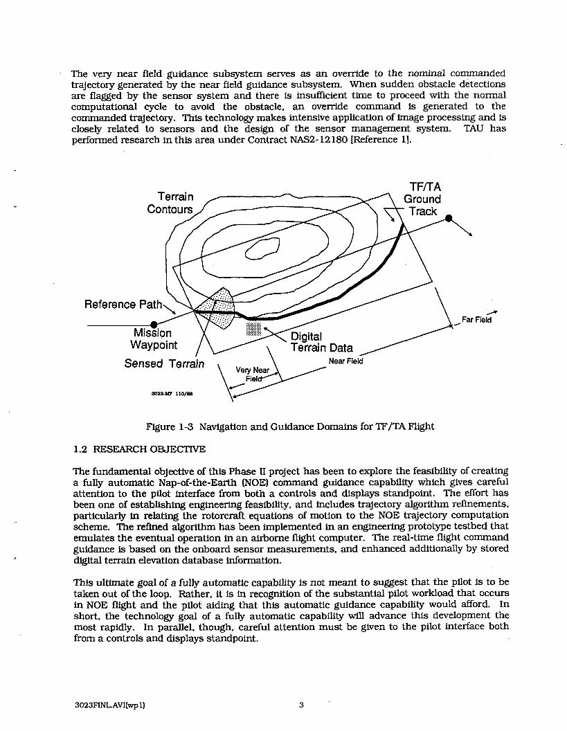
The very near field guidance subsystem serves as an override to the nominal commanded trajectory generated by the near field guidance subsystem. When sudden obstacle detections are flagged by the sensor system and there is insumcent time to proceed with the normal computational cycle to avoid the obstacle, an override command is generated to the commanded trajectory. This technology makes intensive application of image processing and is closely related to sensors and the design of the sensor management system. TAU has performed research in this area under Contract NAS2- 12 180 [Reference 11.

Terrain Contours

TFrrA 7 Ground

9 Field

Sensed Terrain

30x3-M7 ll0las

Figure 1-3 Navigation and Guidance Domains for TF/TA Flight

1.2 RESEARCH OBJECTIVE

The fundamental objective of this Phase I1 project has been to explore the feasibility of creating a fully automatic Nap-of-the-Earth (NOE) command guidance capability which gives careful attention to the pilot interface from both a controls and displays standpoint. The effort has been one of establishing engineering feasibility, and includes trajectory algorithm refinements, particularly in relating the rotorcraft equations of motion to the NOE trajectory computation scheme. The refined algorithm has been implemented in an engineering prototype testbed that emulates the eventual operation in an airborne flight computer. The real-time flight command guidance is based on the onboard sensor measurements, and enhanced additionally by stored digital terrain elevation database information.

This ultimate goal of a fully automatic capability is not meant to suggest that the pilot is to be taken out of the loop. Rather, it is in recognition of the substantial pilot workload that occurs in NOE flight and the pilot aiding that this automatic guidance capability would afford. In short, the technology goal of a fully automatic capability will advance this development the most rapidly. In parallel, though, careful attention must be given to the pilot interface both from a controls and displays standpoint.

With this in mind, the work on this contract has been oriented towards developing a manned simulation capability for NOE command guidance, with the pilot respondmg to guidance displays generated by the logic to "close the loop" manually. The algorithms have been implemented on the NASA-Ames "fixed-cap" real-time simulation facility and a significant level of refinement to the software has occurred as a result of a series of real-time simulations.

A second objective of this project has been to automate the technique of selecting flyable NOE routes. A microcomputer-based mission planning workstation has been designed, developed. and implemented for a variety of flight applications. The thrust of this effort has been to perform automatic route and waypoint generation using a dynamic programming optimization tool. The system, itself, is highly interactive allowing the user to integrate a large array of aircraft types, and overlay hazards such as missiles. guns, radar, and weather onto a digital terrain map. The optimum route information can then be provided to the pilot in "Kneechart" or cartridge load up format, or it can serve as the initialization of route data for the NOE guidance algorithm.

1.3 REPOETT ORGANIZATION

This research effort has been organized around two central themes, the far field navigation task of global route optimization, and the near fieldheal-time guidance and navigation which provides for both obstacle avoidance and local trajectory optimization in the NOE environment. This report is accordingly organized along these topics.

In addition, a significant effort was required to obtain digital map data and to apply it to the navigation software. The results of this effort are discussed in a separate section.

2.0 FAR FIELD NAVIGATION - THE DYNAPLAN MISSION PLANNING WORKSTATION

2.1 GOAL

2.1.1 Initial Obiectives

1. The goal of this effort was to utilize a low-cost microprocessor-based host, specialized high-resolution graphics boards, an emcient user input device, and related interactive interfaces to produce a standalone, low-cost mission planning workstation.

2. The following is summary of the actual IBM AT-based Mission Planning Workstation System which was demonstrated. The development path was one of designing modular software components which lend themselves to many typical workstation concepts.

3. The near term goal of the mission planning system was to access a DMA sourced map display and manipulate it with selectable icons pictured above it. Via a mouse, the user points to a select icon which represents such items as threats and waypoints. Now pointing to a map position. he will overlay it on the terrain map. In this way, a mission scenario is quickly created, and thus transferred to the mission planning software module.

4. A set of optimum solutions will then be computed and stored, with a best route being returned to the executive software module. Alternative starting points can then be designated, and new routes quickly retrieved.

5. The next developmental stage consisted of generating companion X-Y plots of route- relevant information such as cost versus distance, fuel considerations, etc. Also, an interactive commanded route designation process had to be implemented. This commanded route was batch generated and the related costs and plots were produced and displayed by the system.

6. The third development step consisted of refining the system through pull-down windows, more detailed threat models, the capability of moving user-selected points (versus adding and deleting), and accessing some of the detailed data of the mission planning model (threat characteristics, grid sizes, vehicle performance characteristics, etc.).

7. This development effort had five subcomponents:

DMA Map and Cost Grid Handling

Mouse-driven inputs used to profile the mission planning parameters including threats

Mission planning software interfaced to Dynapath workstation executive.

Flight plan smoothing module design and integration

Interactive display of mission planning solution data.

2.1.2 Current Configuration of the Far Field Mission Planning Workstation

This summary describes the development efforts on Dynaplan, over the period of performance.

These achievements include:

Assignment of a single dynamic programming cell resolution which provides both adequate resolution for the optimization process, yet is not too large for the memory of the host computer nor requires an excessive computation time.

o Development of a flexible data compression algorithm

e ~ntegration of a map data management capability

Display of commanded waypoints and sequential re-optimization

e Optional optimization with respect to enroute targets of opportunity

Creation of a threat database management module

o Design of an interactive cost adjustment module

On-line rapid computation of terrain masking

Generation of a prototype Mission Plan listing

Integration of an image processing module to enable map registration and feature extraction capability.

The Mission Planning Workstation and its interfaces are shown in Figure 2-1. This system is hosted on an IBM PC-AT and runs under the DOS operating system. Additional PC boards have been added to support the extensive high resolution graphics and image processing capabilities. Nearly all functions are implemented using a mouse which serves to let the user point at icons designating functions and data displays.

DATA TAPE &.....a

VIDEO

NETWORK

' 1 1 /----"-----\ I DATA TRANSFER MODULE

- COMPACT DISK

3023-MPS 10188 I DATA K0UISITK)N *THREAT ANALYSS I IUW EXPLOITATDN a MlSSlON PLANNIW I

Figure 2- 1 TAU Mission Planning and Image Exploitation Workstation

~O~~FINL.AVI(W~ 1) 6

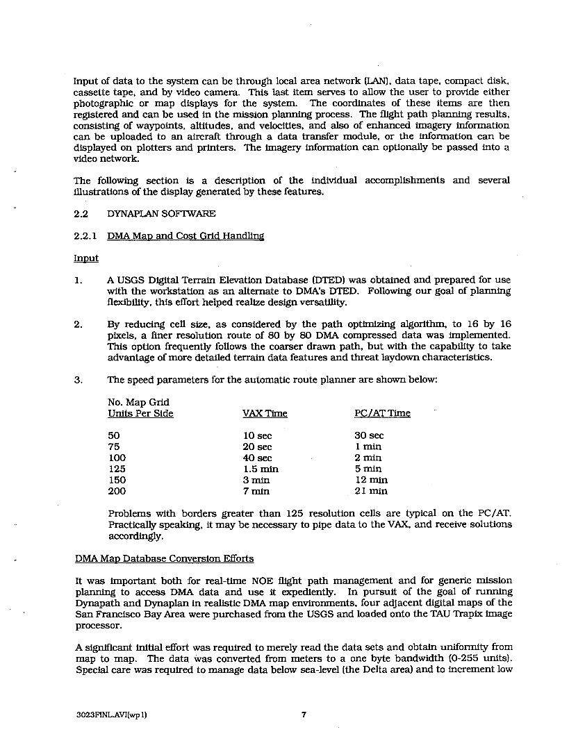
Input of data to the system can be through local area network (LAN), data tape, compact disk, cassette tape, and by video camera. This last item serves to allow the user to provide either photographic or map displays for the system. The coordinates of these items are then registered and can be used in the mission planning process. The flight path planning results, consisting of waypoints, altitudes, and velocities, and also of enhanced imagery information can be uploaded to an aircraft through a data transfer module, or the information can be displayed on plotters and printers. The imagery information can optionally be passed into a video network.

The following section is a description of the individual accomplishments and several illustrations of the display generated by these features.

2.2.1 DMA M ~ D and Cost Grid Handling

1. A USGS Digital Terrain Elevation Database (DTED) was obtained and prepared for use with the workstation as an alternate to DMA's DTED. Following our goal of planning flexibility, this effort helped realize design versatility.

2. By reducing cell size. a s considered by the path optimizing algorithm, to 16 by 16 pixels, a finer resolution route of 80 by 80 DMA compressed data was implemented. This option frequently follows the coarser drawn path, but with the capability to take advantage of more detailed terrain data features and threat laydown characteristics.

3. The speed parameters for the automatic route planner are shown below:

No. Map Grid Units Per Side VAX Time PC/AT Time

10 sec 20 sec 40 sec 1.5 rnin 3min 7 rnin

30 sec l m i n 2min 5min 12 min 21 min

Problems with borders greater than 125 resolution cells are typical on the PC/AT. Practically speaking, it may be necessary to pipe data to the VAX, and receive solutions accordingly.

DMA M ~ D Database Conversion Efforts

It was important both for real-time NOE flight path management and for generic mission planning to access DMA data and use it expediently. In pursuit of the goal of running Dynapath and Dynaplan in realistic DMA map environments, four adjacent digital maps of the San Francisco Bay Area were purchased from the USGS and loaded onto the TAU Trapix image processor.

A significant initial effort was required to merely read the data sets and obtain uniformity from map to map. The data was converted from meters to a one byte bandwidth (0-255 units). Special care was required to manage data below sea-level (the Delta area) and to increment low

lying sea shore terrain so that the accompanying color look-up table would correctly designate the coastline.

Jointly, these maps cover an area of 2401 by 2401 cells with a grid point at every 3 arc seconds of earth angle. This spacing is equivalent to appmximately 100 meter spacing in the N-S direction and about 80 meter spacing in the longitude direction. The actual area stretches over 120 by 96 nautical miles from 36-38 degrees North latitude and 123-121 degrees West longitude.

The maps are now available as image files and as direct access files for use on the NASA system. In addition, the overall map has been compressed to a smaller size and has been adjusted for latitude to be shown in the appropriate square scale. This image has been transmitted to the Dynaplan system on the IBM-AT computer.

Dynapath trajectories were then generated using this data and waypoints were derived from the Dynaplan system.

In addition to Digital Terrain Elevation (DTED) Level 1 (3 arc/secondsj, Level 2 maps were assessed for data conversion into standard formats accessible to both Dynaplan and Dynapath.

2.2.2 Threat Masking

Threat Database Management Module

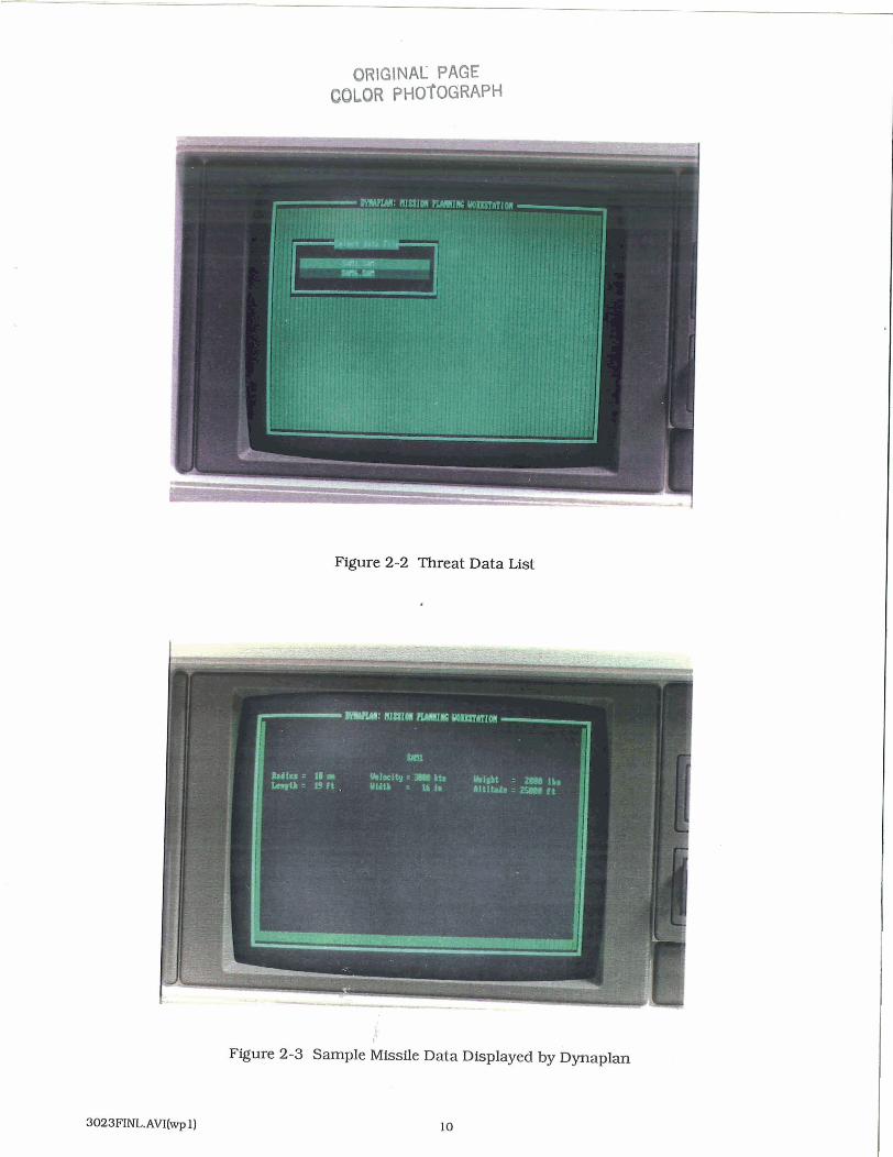
The key threat elements used in this version of the Dynaplan software are weather, missile systems (surface-to-air), anti-aircraft artillery 0, and surface-based radar. The initial software dealt with the proof-of-concept of these threats by providing for generic threats which have representative ranges. This module of the program was then expanded to allow the insertion of a large catalog of applicable systems. Further efforts in this part of the development enable providing a detailed description of each threat element and a convenient user interface to this data. When the operator uses the mouse to point at a generic threat type. the current software lists all the specific threat types on the system display.

Figure 2-2 is an illustration of how this appears. When the mouse pointer is clicked over the missile icon, the system display lists the particular missile types stored in the system. The mouse cursor can be directed to this display to enable the user to designate (by clicking the positioned cursor) specifically which threat model is to be employed. When the SAM6 data- type was selected, the available information on the system was then displayed for confirmation. As shown in Figure 2-3, this data can include and surpass the data requirements of the Dynaplan software. The data, however, can be linked into a larger system for use by operations peripheral to mission planning. The data can be edited, deleted, and otherwise modified rather easily using the "Oracle" database management system.

ThreaUTerrain Data Integration

A data manager is being developed to coordinate threat intervisibility, threat/terrain masking, and their relative weights in the routing process. Visibility with respect to known threats had to be computed quickly and iteratively. These calculations include the averaged aspect angle of the vehicle with respect to the threat for each of the candidate controls. Nominally selected aircraft flight clearance is a necessary input for this, along with maximum detection range calculations for both acquisition and tracking.

On-Line R a ~ i d Com~utation of Terrain Masking

The method of computing line-of-sight terrain masking of the threat with respect to the selected aircraft flight altitude was slightly modified to increase the speed of the optimization process. The revised software now concurrently updates the pertinent dynamic programming cost data array as the terrain masking computations are performed. This technique slightly slows the display generation, but greatly reduces the time required to generate a route. In addition. a software toggle has been introduced which can let the operator locate all the threats without performing any masking computations. The scenario can be stored and edited rapidly. An interior check by the software prevents the user from attempting to generate an optimized route without first resetting the toggle and performing the masking calculations.

Figure 2-4 shows the effect of terrain masking on a selection of missile and radar threats. Entire quadrants of the coastal radars are obscured by the relatively steep terrain. Note also that these computations are performed with respect to the selected flight altitude of the aircraft. If a flight level of several thousand feet were commanded, little, if any terrain masking would be evident.

2.2.3 Commanded Wawoints and Route O~timization

Commanded Wavpoints

A significant enhancement to the mission planning capability was developed with the development of a method of allowing the user to command waypoints through which the system must fly, yet where the optimization algorithm is enabled. Figures 2-6 and 2-7 demonstrate how this technique is implemented. In Figure 2-5, the user has selected the commanded waypoint icon (the 4th icon from the left in the row of icons) and positioned the white square over two locations on map display. Each time the mouse button was clicked, the icon was frozen and numbered on the display. Next, the ROUTE PLANNER (upper left comer of the display) box was selected to activate the route optimization procedure. This was verified to the user by changing the color of the box from the nominal green, to white.

ORIGINAL PAGE COLOR PHOTOGRAPH

Figure 2-2 Threat Data List

4

Figure 2-3 Sample Missile Data Displayed by Dynaplan

ORlGlYAC PAGE COLOR PHOTOGRAPH

Figure 2-4 Terrain Masking of Threat

I,

Figure 2-5 Commanded Waypoints

In Figure 2-6, the optimization has been completed (approximately 20 seconds of computer time are required), and the sequentially optimized legs of the route are drawn to the display. Note that the flrst leg goes from the start point in the west straight over the northern part of the San Francisco peninsula, and then directs the aircraft over the bay to the waypoint. The next leg of the route heads over the pass to the ocean, staying at the coastal elevation until the course must head inland to pass through the second commanded waypoint. The last leg of the route winds through another mountain pass to reach the destination.

If the results of this segment of the effort are carefully analyzed, it becomes clear that the Dynaplan algorithm became an ideal tool for automatically generating the coarse/global route segments which are then refined in the real-time trajectory generation Dynapath software.

O~timIzation to Enroute Targets of O~~or tun i ty

Another refinement to the mission planning capability has been the introduction of incentives to encourage the optimization algorithm to pass the route through or near selected points. DifTerent from comxnanded waypoints, these enroute items may be additional targets or reconnaissance opportunities. Figure 2-7 illustrates an optimization where the goals are terrain elevation minimkation with a large collection of candidate enroute targets in the region surrounding the starting point and the destination.

Figure 2-8 is presented to illustrate the level of precision with which Dynaplan negotiates a combination terrain minimization and threat avoidance path to the destination. Commanded waypoints are subsequently assigned for an alternate solution.

Figure 2-9 includes the commanded waypoint solution and suggests the ease with which an operator can design both the ingress and egress to a target.

A key feature which accounts for significant program speed is the technique of varying the specification of the grid density and geometric bounds of the database, even though the graphics board maintains a high fidelity display. To perform this, a data compression algorithm fllters the database, and can either average or maximize the attributes of the underlying cells into the sparser grid. The solution is then translated into the projected display using both positional values for the offset of the map, and an appropriate zoom factor. (See Section 2.2.5 for more detail.)

Program OutDut and Follow-On Develo~ment Goals

After generating the optimbed solution. there remains a wealth of useful data which can be extracted and displayed. The "cost-to-go" from every point in the dataspace to the fixed point (goal) resides in an array. An algorithm which is under development will histogram the values. develop a gray scale map and color lookup table, and then plot this over the existing map. In this way, the various possibilities can be displayed in a meaningful way.

Another post-optimization tool generates a strip chart of the range/altitude profile for the optimum trajectory. With further development, time, threats, and other data can be factored into the plot as a guide to visualizing the route. The terrain masking altitude, clearance altitude, and implied climb/descent angles should be clearly indicated.

ORlGlNeC PAGE COLOR PHOTOGRAPH

Figure 2-6 Optimization Through Commanded Waypoints

I '

Figure 2-7 Optimization with Enroute Targets

ORIGINAL PAGE COLOR PHOTOGRAPH

Figure 2-8 Route Optimization in the Presence of Several Threats

i

Figure 2-9 Alternate Route Through Commanded Waypoints

Another capability which has been developed allows a user to specify (via mouse), a series of points that it is desired a route should pass. These may include navigation waypoints, intermediate targets or objectives, refueling points, and target initialization points. The route planner program then draws the route using straightline segments and evaluates various parameters such as:

Path cost using the optimization metric Total distance Enroute time and fuel required Cumulative Probability of being detected - if modeled Cumulative Probability of being killed - if modeled

The above function serves as an excellent training aid, and will also help to provide the user alternatives for establishing the relative weights used in the cost model for the optimization. The software will interactively allow the user to modify the route by moving commanded route points, and quickly learn their mission implications.

2.2.4 Data Manarsement

Dvnamic Programming Cell Resolution

The dynamic programming cell resolution was selected to consist of 60 lateral, 60 vertical, and 8 control cells. This correlates with a 5: 1 data compression, in both horizontal and vertical directions, with respect to the actual map display on the graphics board. The selection of the cell size depends upon the speed and maneuverability of the aircraft employed in the technique. The 8 control method presumes that the aircraft can enter a programming cell along any of the control directions and can exit along any other direction. Therefore, the cell space should at least accommodate 90 deg. turns by the aircraft.

Mission Plan Listing

The ultimate use of an automatic mission planning tool is to produce a usable set of information for the pilot and aircraft avionics system. A simple prototype of pilot output has now been created. The optimized route can now be sent either to the system display monitor or to an attached printer. Figure 2-10, a sample pilot kneechart, lists the legs of a derived mission. Included in the list are leg coordinates in latitude/longitude measures, aircraft heading data, distance, time, and fuel components, and altitude and velocity data. Wind and magnetic deviation tables are referenced to derive ground speed and magnetic headings.

The flight log serves only as a prototype since most potential users have individual preferences for the content and format of the route information.

Figure 2- 11 displays the terrain profile (white) and the aircraft flight profile (red) along the optimized route. In this illustration, the aircraft is assigned different barometric altitudes to fly for each of four legs of the mission.

Interactive Cost Adiustment Module

The concern for various elements in a mission scenario may be highly subjective. For example, a medium weather system may be scrupulously avoided by an ill-equipped aircraft, yet be sought as an element for concealment by an aggressor.

ORIGINAL PAGE COLOR PHOTOGRAPH

Figure 2- 10 Sample Flight Log

5

Figure 2- 1 i Terrain Elevation Pmfile

ORIGINAL PAGE- COLOR PHOTOGRAPH

Figure 2- 12 Interactive Cost Adjustment Module

t

Figure 2- 13 Removal of Terrain Avoidance as an Optimization Measure

The Dynaplan system has been designed accommodate this variability by allowing the user to quickly and easily designate his relative concerns with elements of the scenario. Figures 2-12 and 2-13 show, in icon format, the features which are available to the principal planning - display. Above each, a vertical bar is provided to permit the user to adjust the relative value of each item. By pointing the mouse cursor at a bar, the height of the bar can be raised or lower within the display limits. Since the values are only relative to each other. there is no need to quantiFy these elements. Note also that two bars are oriented in a negative direction. This allows the user to indicate the relative degree of attraction, rather than adversity, which may be specified to either of two classes of enroute targets. Note in Figure 2-13 that the rightmost icon, which pertains to the terrain avoidance factor, has had the vertical bar depressed to the origin, and consequently is flagged by a change in the icon color. This indicates that this factor is no longer a measure in the optimization.

Smoothing

In determining the globally optimum trajectory, the far-field navigation algorithm. Dynaplan, generates a dense set of data points which connote the best path from start to end. If directly applied as waypoints to the near-field navigation algorithm. Dynapath, the proximity of the points and the coarseness of the individual headings derived these points would "oversteer" the algorithm by forcing it through closely spaced points which were generated using a terrain and threat data grid which is far coarser than that which is employed in the near field.

The auto-smoothing algorithm accepts the Dynaplan generated trajectory and a set of parameters and weighing factors. It then determines a subset of points from the original data set which closely follows the original. The degree to which the original points are thinned is dictated by several input parameters. The basic parameters are time interval between waypoints and the amount of deviation allowed. The weighing parameters assign the relative importance of each. For the example shown in Figure 2-14, the desired waypoint separation was set to 10 minutes and the deviation threshold value 0.5 nm. The weighing parameters were set at 5 for waypoint intervals and 75 for the deviation. Thus. the importance of closely following the optimized route greatly outweighed the emphasis on waypoint intervals.

The smoothing algorithm proceeds as follows: starting with the initial point in the Dynaplan generated trajectory, the algorithm evaluates the successive points as candidate waypoints. It generates a figure of merit for each candidate by multiplying the difference between the actual and desired waypoint separation by the length weighing factor (5 in the above example), and the maximum deviation of the actual points along the route in excess of the threshold (0.5 nm in the example) and the candidate by the deviation weight (75 using the sample above). The candidate with the lowest score is selected as the smoothed waypoint and the process then reinitializes to this point and continues. As the procedure nears a terminus (which may either be the end point of the trajectory or a commanded waypointl. it also measures the distance-to- go, and penalkes deviations from this distance and the desired segment length by the length factor and adds it to the figure of merit. This last measure serves to prevent the algorithm from selecting a very short last leg. In intuitive terms, it gives the algorithm foresight.

Figure 2-14 illustrates the smoothing process applied to a rotorcraft operating over a 173 nrn route. The assigned speeds along the way vary between 40 and 120 kt, and the commanded flight altitudes range between 30 and 100 feet (AGL). The total flight time for the missionis 2 hours and 8 minutes. The algorithm derived a subset of 23 points from the original 84. The key inflections of the original route were maintained adequately. In this figure, the original route is shown in solid and the smoothed route in dashed lines. Plot markers denote the original commanded waypoints and the waypoints generated by the smoothing algorithm. The terrain contours are for the San Francisco Bay area.

COMMANDED WAYPOINTS

WAYPOINTS

SMOOTHINQ ALGORITHM

SM00lUED ROUTE

DASHED LINES

Figure 2- 14 Automatic Route Smoothing

Figure 2- 15 Sample Dynapath Corridors

Figure 2- 15 illustrates how route segment boundaries could be automatically placed about the smoothed data set for Dynapath implementation. The width parameters could be assigned based upon the maximum measured deviation in each segment and the uncertainty of the Dynaplan data base. For example, if the grid used in the Dynaplan algorithm contains cells 0.5 nrn across and the maximum measured deviation measurement in the smoothing process were 2.5 nm, then the segment width should be at least 3.0 nm. This corresponds to about 5 Inn or 50 cells measured at the typical 100 meter interval used in Dynapath.

2.2.5 M ~ D Management

Data Commession Algorithm DeveloDment

A map data compression routine was developed which allows the user to represent the terrain in the dynamic programming grid with a value which can be selected anywhere between the average and the maximum values of the data points in each cell. This compression process is useful in allowing the mission planner to provide for terrain avoidance as an absolute constraint or as a statistical measure. By selecting the maximum value as the compression parameter, the terrain grid uses the highest terrain point in the programming cell as the representative value, thus denying possible routes through areas where only a small feature may be high. Selection of a lesser value (75% of max has been shown to work well) is equivalent to assuming that the aircraft can maneuver through a cell which has a locally high point. Selection of the maximum as a constraint may be appropriate for poor visibility conditions, while a relaxation of the constraint might be more suitable for high visibility conditions or scenarios where the a~craf t is presumed to be equipped with on- board terrain sensors.

Map Data Management -

Several digital terrain data tapes in DMA format were both joined and compressed on the TAU VAX computer. The data was then transmitted to the Mission Plannhg Workstation. Figure 2- 16 illustrates the results of this effort. It is worth mentioning that the data is greatly enhanced by selection of an appropriate color lookup table. If the digital data were merely presented as a grey-scale display where the terrain elevation were a shade of black or white as determined by the 8-bit resolution of the display, the shore line would be indiscernible. An intermediate algorithm was employed to both accent the ocean and to highlight the mountainous terrain.

Other Dynaplan developments represented in Figure 2-16 include automatic computation of the latitude and longitude coordinates wherever the mouse pointer is positioned. These values are shown (in degree/minute/second format) on the bottom of the display. The border of the map also includes labeled tick marks for the major map coordinates. (They are incorrect in the figure, however this error has since been corrected).

Finally, the optimized route which is exhibited in the figure illustrates the terrain elevation minimkation nature of the optimization algorithm. The route stays over water as long as possible and then winds through a mountain pass enroute to the designated target. The slight 45 degree bends in the over-water portion of the route illustrate the relationship of the dynamic programming cell size to the map display.

ORIGINAL PKGT COLOR PHOTOGRAPH-

Figure 2- 16 Translation of Screen Coordinates to Earth Angles

3.0 NEAR FIELD NAVIGATION - THE DYNAPATH SOFIWARE

3.1 INTRODUCTION

One of the major efforts of the Optimal Guidance Phase I1 effort was to further develop the technology of near field navigation. The near field flight domain requires solving for optimal or near optimal flight path and the consequent aircraft control commands for approximately the next 30 seconds of flight. This time interval is of particular concern because it will typically be using a fusion of long term information (digital map data, known threats, waypoints, etc.) and near term data supplied by on-board sensors (pop-up threats, unmapped hazards, and cultural features). Trajectories must be determined which minimize the risks of exposure and collision, are optimized with respect to the destination (time, fuel, etc.), and are flyable by the aircraft and pilot.

Development of an extensive set of algorithms, Dynapath, is one of several potential technolo- gies which have application in the TF/TA/NOE flight environment. Dynapath has been proven, in principle, to be an optimal control approach that can be implemented in real time.

Dynapath is a set of automatic command guidance algorithms which was developed for low altitude/high performance aircraft flight at altitudes of 100-500 feet. A number of enhance- ments and modifications to this software were initiated under another contract (Ref. 11, but the most significant developments for real-time implementation have occurred during this Phase I1 effort.

3.2 OVERVIEW OF DYNAPATH TF/TA OPTIMIZATION

Before describing the modifications made to the Dynapath software, it may be useful to provide a brief description of the trajectory optimization process and to describe the components and interfaces of the Dynapath algorithms. Additional detail can be found in the References 1.3. 4, and 5.

In a mathematical sense, the definition of the near-field navigational problem is to find the 3-D trajectory in inertial coordinates which corresponds to a minimum of an optimization perfor- mance measure. The trajectory is subject to the following conditions:

the initial boundary conditions and velocity vector are given;

the final boundary conditions may be relatively unconstrained;

the helicopter equations of motion must be satisfied;

the trajectory must satisfy a range of parameters such as terrain clearance, both laterally and vertically, flight path angle, maximum bank angle, and total acceleration (g-load).

Furthermore, the solution trajectory must have the following features. It should be globally optimal to satisfy the tactical flight objectives. The computations of individual trajectory segments must reflect the employment of an adequate look-ahead to avoid major obstacles. For example, box canyons should be seen within a single patch computation. Additionally, unavoidable ridgelines require sufficiently early detection to initiate a climb rate within the aircraft limits.

Other operational features important to the solution are that the trajectory segments maintain continuity through the flrst derivative as a minimum. Step changes in the veIocity vector are

obviously unflyable and bear no approximation to any aircraft capabilities. Continuity of the acceleration profile guarantees an even closer approximation to the performance of an aircraft. For example, a helicopter in a maximum banked turn to the left. cannot immediately reverse itself and turn to the right. It is limited by its roll agility and, in an NOE environment, the need to maintain sufncient lift to avoid critical loss of altitude. To the same extent, then, the optimization process should generate trajectories which are fully compatible with the flight control system. In general, it has been found that the trajectory and control settings should be provided to a resolution of one second. This time scale is of the order of pilot and aircraft/control response.

Another feature of the solution process required for successful implementation in a flight system is that the method lend itself to real-time operation. The Dynapath algorithms guarantee a solution within a predictable time.

Performance Measure

The TF/TA trajectory computation is based on Dynamic Programming techniques. As in all such approaches, it is necessary to first define a performance measure, or cost functional, against which possible trajectories are ranked and selected. Whereas the global trajectory relates to higher level mission goals, the objective for the real-time trajectory computation is more microscopic or near-term in nature. The TF/TA valley seeking performance measure used in the Dynapath algorithm is shown in Figure 3-1. This measure uses the global trajectory as a baseline for developing the fine-tuned trajectory, in that lateral deviations from a global trajectory are penalized, while flight at higher altitudes is also penalized. In evaluating all possible trajectories using this penalty function, the best trajectory generally seeks out low altitude corridors ('Wleys") in the neighborhood of the global reference trajectory. The relative weight between these penalties is called the TF/TA ratio. A large value for this ratio results in essentially TF flight along the reference trajectory, thus bypassing low altitude corridors, while a small value would permit large deviations (TA flight) in the search for low altitude corridors.

The general philosophy behind this performance measure is that low altitude corridors afford terrain masking from threats, and thus represent good candidates for improvement over the global reference trajectory. Threats and terrain masking should also be incorporated explicitly for best performance. Otherwise the TF/TA trajectory may go through a threat region unnecessarily. Mathematically, inclusion of threats can be achieved by adding to the TA/TA performance measure a term P (P&. associated with the threat danger Pk in cell i.

The optimum trajectory is determined by summing the incremental costs associated with each step, or time interval, in the trajectory. The connected set of steps with the minimum total cost is the optimum.

Dyna~ath Functional Descri~tion

A functional block diagram of the Dynapath TF/TA algorithm and Command Generators is shown in Figure 3-2. The TF/TA algorithm computes a horizontal or lateral path solution to the trajectory which optimizes the performance measure in the vicinity of the reference ground track. The horizontal solution is handed off to the Vertical Path Generator for an optimization of the TF/TA trajectory over the terrain data associated with the horizontal path. Both solutions result in a computation of consistent commands for the state derivatives.

PERFORMANCE MEASURE MFINIW. HOSTILE DEFENSES CAN ALSO BE INCLUDED

TF/TA Compu

cnntn~ Terrain ~r?: E

Threat Template

Sensed Terrain

Key TF/TA calculations within a patch

Patch is scrolled downstream periodically and calculation repeats

Waypoints require special treatment

\ Cell i

\ I I 7 i Set Clearance Altitude

Figure 3- 1 Patch Computation Performance Measure

This decoupled approach to trajectory generation wherein the horizontal and vertical paths are separately optimized is a simplification of the overall 3 degree of freedom trajectory optimiza- tion. The benefit of this procedure is the reduction in computational complexity. The method assumes the aircraft can simultaneously perform within both horizontal and vertical maneuvering limits.

I n ~ u t s and Modules

A major input to the algorithm is the digital terrain elevation data. This data is smoothed in a pre-processing step, which applies safety factors to keep the algorithm from selecting trajectories too close to high frequency peaks in the terrain.

The Horizontal Path Generator (provides a ground track as specified by set of closely spaced ground track points (q,yo). (xi ,y1). . . . . (xn;Yn). This smoothed command ground track is sent to the Vertical Path Generator, which computes all the vertical command states. The speed may vary as a function of the vertical flight profile, depending on the aircraft model used. For a constant energy model, the speed Vc is not known until after computation of the vertical commands. A constant velocity assumption was used for the NASA-NOE simulation environment. Within limits, the capability for constant velocity is assured by Umiting the climb/descent profile in the algorithm compared to the true helicopter maneuverability.

The Vertical Path Generator module receives the terrain profile associated with the horizontal path solution and optimizes for the TF/TA/NOE trajectory which most closely follows the terrain subject to the set clearance altitude constraint and the aircraft maneuverability limits. The profile is illustrated in Figure 3-3.

The inertially referenced commands are then passed through to the pitch-roll decoupler. This provides an interface to the flight control system and serves a tracking function of guaranteeing adequate authority to the vertical channel to maintain altitude, while assuring that lateral deviations from the commanded trajectory are minimized.

Figure 3-3 Vertical Solution Procedure

3.3 THE DYNAPATH TF/TA/NOE ALGORITHM

The Dynapath algorithm is a mixture of Dynamic Programming (DP) and tree searching. The tree structure has been implemented in a way which minimizes the amount of computation associated with the kinematics of the aircraft and the Dynamic Programming to selectively reduce the number of possible trajectories. So, basically, the problem is solved by a simple forward running Dynamic Programming algorithm where the state transitions are handled by a tree structure.

The advantage of this technique is that it guarantees a smooth trajectory which has no discontinuities in the position or the velocity vector. Further, a considerable number of non- trivial methods exist for directly computing the aircraft controls from the resultant trajectory parameters.

Ground Track Com~utation

The ground track is found by essentially assuming that the aircraft can fly perfectly in the set - clearance surface. This surface is a surface above the smoothed terrain surface but displaced by a constant set clearance bias. The TF/TA tradeoff is made under this assumption, resulting in the lateral ground track. The vertical command generator then relaxes the assumption that the aircraft flies perfectly at the set clearance altitude, and treats the set clearance altitude as a minimum altitude constraint.

In computing the set of potential maneuvers of the aircraft, we start with a consideration of coordinated turns. The two dimensional trajectory of the aircraft is a function of speed and bank angle. A change in the bank-angle in turn affects the reciprocal instantaneous radius of curvature p.

A time scale quantization of one second is a suitable unit for the framework of assigning maneuvers since an aircraft typically requires 1-2 seconds to roll from one banked turn maneuver to another. One second is also consistent with the frequency with which a pilot can accept and execute individual flight correction commands.

In Dynapath, five bank angles are typically used to represent the aircraft at discrete lateral maneuvering capabilities within its performance limits.

A five state tree and a corresponding discretization in time of 1 second, which is approximately how long it takes to go from one state to a neighboring state were also found to be suitable in tenns of finding solutions in a real-time computing environment. Note that a finer quantization in time would cause the tree of possible trajectories to increase--with corresponding computational increases--while coarser quantization in time will be seen to undersample the performance measure, the latter being associated with the terrain data.

The reciprocal radius of the turn radius p=l/r functions as the control variable. Note that this measure doesn't vanish with zero bank angles and can be expressed relative to gravity (g). velocity 0 and bank angle ($) as:

Trees are generated using p a s the control variable. All possible discrete values of p are used initially to exhaustively generate every branch of the tree for the next several seconds associated with generating a tree of possible trajectories. Each node of the tree corresponds to

a time increment (typically 1 second) from the previous node. At each node of the tree, the following information is stored:

Position (x,y)

Heading yf

The parent node identification

The cumulative cost of the trajectory to the present node

The curvature control used to arrive at the present node

Every time a new node is generated, the new node is computed using the parent data and incremental position and heading data associated with the curvature control which is applied.

The curvature controls correspond to the bank angles selected for the maneuvering of the aircraft. They are typically quantized in five values corresponding to the maximum bank angle in each direction, half the maximum bank angle, and straight flight.

The corresponding controls a& referred to as: 0, +1, &!2 where negative controls direct a right turn and 22 directs use of the maximum permissible bank angle.

Because of limitations on the roll-acceleration of the aircrait, p is limited as to how much it can change at each transition. Accordingly, p can only change by one control measure at each tirne interval. also, the ltrl controls are often used as transition states requiring the next control selection to continue descending/ascending as dictated by the previous command.

Constraint Pruning Within the Tree

Given an initial position. heading and curvature. Dynapath constructs a complete tree representing all acceptable paths that the aircraft can follow for the next N seconds. Note that N is the level number of the tree (the depth) because each node transition represents 1 second. At tree generation tirne, branches can be discarded according to several possible criteria prior to a cumulative cost comparison. The use of such criteria is denoted as constraint pruning. The speciflc criteria used in Dynapath are:

a. A node under consideration must not exceed the maximum lateral deviation from the reference path.

b. The heading at the end node of a tree must lie within a user-specifled angle range measured from the reference path direction.

c. The end node of a tree must exhibit net forward progress along the reference path with respect to the starting node of the tree.

Dynamic Prollramming Overlav

The end nodes of the initial and later trees are classified into a Dynamic Programming "overlay," as shown in Figure 3-4. This is shown as a rectangular grid that is oriented along the reference track. Subdivisions are indicated as a three-dimensional spatial classification of the space according to the zone, division, and heading dimensions. The heading subdivisions are divided according to an angular classification into one of several possible cells (possible azimuth directions).

Figure 3-4 Dynamic Programming Overlay

The number of zones, divisions, and heading subdivisions are selected to correspond to the degree of pruning which is desired. The coarser the resolution of the overlay, the more aggressive will be the pruning process. With fewer subdivisions, fewer candidate paths survive the pruning process to start new generations of trees. Conversely, as the number of partitions is increased (smaller increments in zones, divisions, and/or headings) fewer candidate trajectories will be compared in each cell in the pruning process. As a result, more paths are retained to propagate new generations of tress. A greater number of potential paths can therefore be compared in selecting the overall optimum trajectory.

The increase in number of paths generated, however, proportionally increases the degree of computation required in generating a solution. When the Dynapath algorithm is used as a . real-time component for path optimization, the cell sjze must be balanced to the computer processing rate. Typical subdivisions currently used on the NASA MicroVAX computer uses about 20 zones. 20 divisions. and 5 heading subdivisions.

The zone and division components of the dynamic programming overlay are independent of the terrain data grid which are used in the calculation of the trajectory and its nodes.

There are many trees that are grown rather than one single large tree. It should be noted that each pruning cycle interrupts the process of generating trees and eliminates redundant paths of higher cost. For a given tree, a DP state for an end node contains a label designating the trunk (source) of the end node, the cumulative cost to that end node, as well as state and control information.

O~timization Procedure

Starting from the initial position and heading in the patch, an initial N stage tree is generated. The value of N is typically three to five, i.e., 3 to 5 seconds of flight time. The initial tree

corresponds to approximately 9 to 27 end nodes (if the previous control was 0) and 18 to 60 total nodes including the initial trunk node. Pruning of this tree and subsequent trees will occur according to criteria such as the maximum lateral deviation from the reference track being exceeded. After pruning, new trees are generated from the remaining end nodes. These new trees are pruned in turn, and the process continues. As the tree is generated, the cell corresponding to each end node is computed. If the cell is empty, the end node, including its cost, is registered as being in the cell. If the cell is already occupied by an end node, the cost of the current end node is compared with the previously registered cost and the end node with lower cost is kept. This forms the basis for the Dynamic Programming (DP) operation for selecting the best trees.

Many trees are used by this technique in propagating to the end of the patch. Once the end nodes of the last trees are past the last zone in the patch, the optimal patch is determined by selecting the end node with the lowest cumulative cost.

The optimum path is retrieved by tracing backward through the DP structure until arriving at the initial tree. This is possible because the algorithm keeps track of the source at every stage. The full set of controls in one second quantizations, is available for the each tree due to the way the solution is constructed and stored. The optimal solution is based on the uniform 1 second quantization over the entire patch length due to the manner in which the DP solution is constructed.

Vertical Trajectorv

Once the lateral path is generated, the vertical trajectory must be determined. This process uses a dynamic programming procedure similar to the horizontal path generator. In this case. a terrain following set of deviations are constructed where the terrain values are known by extracting the terrain elevation associated with the (x.y) values of the digital map at each step of the horizontal path. The heading deviations are replaced with flight path increments which are assigned within the climb and descent angle parameters assigned to the aircraft model.

As in the horizontal case, the controls are taken to be path curvature, this time in the vertical plane. Four curvature quantizations are selected corresponding to 2 positive incremental normal g's, zero incremental normal g, and negative incremental normal g. The cunrature control is designated pv, where

(Nz - l)g where Pv = , and Nz is the incremental normal g load. (Eq. 3.3-2)

tlt

Representative incremental normal g loads for a helicopter in a near NOE environment vary between -.25 to +.25.

The states Sk of each node in the vertical tree structure contains:

The cumulative distance along ground track (x.y) Helicopter altitude Flight path angle The identifier of the parent node that generated the current node Cumulative cost up to and including the current node The curvature control

This state vector is completely analogous to that used in the ground track development. The cost can have any functional form that tends to "push down." the trajectory to the set clearance altitude.

Dvna~ath Algorithm Surnmarv

The converted Dynapath algorithm process flow for a single patch computation is shown in Figure 3-5. The 2-D horizontal path generating algorithm first determines the optimum ground track and then employs similar techniques in a separate vertical path generating module.

The horizontal and vertical set clearance values are optimization parameters. as are the user selected TF/TA ratio and the maximum lateral deviation which the algorithm is allowed in searching for the best horizontal trajectory.

The essential flight parameters which affect the Dynapath algorithm are the acceleration relevant terms such as normal load, max bank angle, and roll acceleration, and also the velocity and flight path angle limits.

End Zone Solution

Figure 3-5 Dynapath Process Flow

3.4 DYNAPATH ALGORITHM DEVELOPMENT

{ p c ~ ~ ~ ~ 1 Commands

@- vertical -4 mstr.int Pruning 1 C o d H-1

The enhancements arid modifications of the Dynapath Algorithms for helicopter NOE flight conditions are of several categories. There were changes to the fundamental or core dynamic programming software. These charges enhance the capability of the software for any aircraft flight applications. This modification relates to the operation of the guidance software as a whole. Improved input displays and techniques for turning waypoints are examples of such modifications. Additionally, these were specific program enhancements designed to cope with operations in a real-time computing environment. Software changes in the category either:

End Nodes Best Solution Tree -

(1) served to significantly speed the execution of the process without adversely affecting the quality of the solution; or (2) dealt with key aspects of the man/machine interface.

3.4.1 Core Algorithm Develo~ments

Horizontal Path Generation

During the transition internal where Dynapath modifications were being performed under both this Phase I1 contract and another contract (Reference 1) the algorithm was found to produce an extremely oscillatory trajectory. Because of a limited set of controls and the employment of high performance turns, small course corrections required large impulsive maneuvers. An "Epsilon Control" technique was introduced and found to provide considerable smoothing to the lateral path trajectory generator. The computing "cost" for this technique was found to be appreciably higher than for the baseline Dynapath, and was eventually discarded as a candidate for real-time software implementation in favor of a reduction of control amplitudes.

The idea behind Epsilon controls was to discard the straight-ahead control and alternatively, introduce two controls each of which produces a heading slightly off the centerline. This allowed the DP software to make minor course changes instead of forcing small offsets in the heading to be corrected with a full bank angle correction. In the initial version of Dynapath, a large bank angle control and roll acceleration rate was assumed. Heading changes were assumed to apply roll acceleration to full max bank angle, a maneuver requiring 2 seconds (controls 0 to 1 to 2). followed by 2 seconds of return.* Thus a minor lateral offset would be allowed to drift until a large scale maneuver could return the drift. It would frequently be impossible to maintain a desired heading within 15 degrees.

The difficulty of Epsilon controls is that the computer cost escalates significantly due to the intercontrol connectivity. Either Epsilon control can propagate a half bank angle to either side. thus doubling the number of choices. The computing cost for this is shown in Figure 3-6. Note that when the trees are pruned every 3 generations. the cost is double that of a standard 3 generation level/5-control Dynapath. When the Epsilon controls are extended to 4 generations before pruning, the cost is 6 times the standard Dynapath.

The solution to the dilemma of providing a reasonably smooth ride quality but within a limited DP search time came from limiting the maneuvering extremes of the subject aircraft without limiting the roll acceleration capability. Thus, the helicopter can roll to the half bank angle control in one second without overshoot and either hold the turn, extend to the maximum . bank angle, or return to wings level. The heading quantization was reduced to a few degrees. The cost of reducing the performance envelope is not appreciable since it is not appropriate to go to large bank angles when nying in an NOE or near NOE environment. For example, a helicopter rotor disk diameter of 50 ft whose hub is 10 ft above the skids cannot bank more than approximately 22 degrees in a coordinated (no climb) turn without the rotor tips beginning to protrude below the lowest part of the fuselage. Large bank angle maneuvers could thus pose a significant hazard when flying in a true NOE environment where clearances of obstacles might be by margins of 10 ft . This modification to the horizontal path generation is significaht. The original, aggressive. search technique produced trajectories which were totally unsuitable for manned flight. Constant large bank angle maneuvers in rapid succession are not only fatiguing on the-pilot, they are often unneeded. By implementing factors which accounted for heading towards the

Yrhe intermediate bank angle was merely a transition control between wings level and full bank.

next waypoint and adjusted gradually for drift from the centerline between waypoints, a smoother and more flyable trajectory was obtained.

PATCH LENGTH

Figure 3-6 Number of computations

Vertical Path Generation

The original Dynapath vertical path generation software extracted the terrain profile of the lateral path and solved for the lowest vertical trajectory by generating DP trees with a set of three controls: max pull-up, zero incremental g, and max nose over. The climb and dive angle limits of the aircraft and the terrain clearance attitude served as constraints to prune the nodes during tree generation.

The process served to prove the concept of generating a flyable vertical path, but resulted in an extremely rough ride. Furthermore, a significant portion of the overall code execution time was spent in the vertical path generation module. The initial modifications to the vertical path generation module focused on reducing the number of nodes generated between pruning and in adding an intermediate positive vertical control (40% of rnax acceleration) (Contract NAS 2- 12180). The additional control resulted in a significant increase in "smoothness of ride" and remains in use today. However, the computation time required for vertical path generation. though reduced, was still significantly large due to the large number of paths which were generated. Upon inspection, most of the propagated paths resulted in altitudes far above the terrain clearance altitude and had cost values greatly in excess of the optimum path. It was observed that other propagated paths which were constraint pruned by the set clearance altitude, could have been pruned several generations earlier if it were recognized that the downrange terrain gradient exceeded the maximum angle of climb.

A terrain profile filtering algorithm was introduced which creates a revised set clearance profile to reflect the clirnb and dive limits of the aircraft. In addition, the vertical altitude zones were

assigned parallel to the smoothed set clearance and unevenly spaced (see Figure 3-7) to aggressively prune vertical paths which were distant from the minimum allowable altitude. The introduction of these measures greatly reduced the number of paths without any loss of fidelity in deriving the optimum vertical path.

The vertical path performance measure was further revised to accommodate flying below the smoothed set clearance altitude. Previous to this, Dynapath would fail if the aircraft dipped even one foot below the constraint. A slight penetration of this constraint across a peak might not be a serious breach of the goal of flying safely as low a s possible. The performance measure provides a heavy cost penalty for flying below the set clearance, but was found to accept, as optimum, the brief excursions characteristic of skimming rough terrain. This cost penalty should be varied in accordance with the set clearance altitude being flown. for NOE altitudes of about 10-20 feet, this cost penalty should be exceedingly large to show a preference for any other vertical profile. At higher clearance altitudes (100-200 feet), a 10-foot undershoot should not be regarded as severe, and the cost penalty should be reduced.

The vertical path algorithm could be further modified resulting in less computation than it currently requires for solutions. Since the revised set clearance itself is the lowest flyable profile, the Dynapath vertical path generating algorithm does not really need to explore the use of vertical controls that exceed the minimum selection of control which stays on or barely above the revised set clearance limit. If, at a node, a selection of sequential vertical controls can be made which bring the helicopter to its lowest vertical flight path altitude without going, below the revised set clearance lirnit during the maneuver, then there is no candidate vertical trajectory. or node above that candidate, which can produce a lowest cost trajectory. Thus, the vertical path algorithm should not be required to generate many exploratory paths, and should be able to maintain the optimum profile at every pruning interval.

This logic has not been implemented on the current Dynapath, since the actual coding and debugging process could have jeopardized other major goals associated with the real-time operation of Dynapath in the simulation environment. However, it shows promise of ultimately reducing the overall patch computation time by approximately 20-30%.

3.4.2 Interface Algorithms

Integration of Dyna~ath with the Helico~ter Simulation

In addition to modifying the Dynapath core algorithms to run more efficiently and produce a trajectory characteristic of helicopters operating in an NOE environment, a considerable effort was required to develop software which interfaced the dynamic programming routines with the flight management software associated with operating within a simulation. The Dynapath code requires an executive shell which gathers and translates user defined flight constraints and waypoints into a route with waypoints and boundaries. The manipulation of the lateral path generation algorithm around waypoints required major revisions. Also, the optimization algorithm seeks the best trajectory for only a point, neglecting the fact that helicopters have a considerable dimension and require a safe horizontal clearance from obstacles. Solutions were found for these and other problems and are discussed below:

Wawoint Management

During the initial modifications to the software, the waypoints which signified heading changes were defined as circular areas with individually specified radii which could be assigned values anywhere between zero (a point) and the width of the route segment. The last computation patch in each route segment was allowed to continue past the waypoint and maintain the same heading. Though there were other software adjustments within this code whose purpose was to promote rounding the waypoint and adopting the next heading, there were constant problems which would often result in the selection of a trajectory which would not be able to stay within the boundaries of the new route segment during the next patch computation.

During the October 1986 real-time simulation. Dynapath could only turn waypoints with heading changes of up to approximately 70 degrees and for helicopter speeds of no more than 60 knots. Larger t u n s were unacceptable. The algorithm had some difficulty in managing to both cross waypoints and pick up the new commanded heading. The problem stemmed from conflicting gains which forced the trajectory through the waypoint and those which drive the trajectory onto the new route heading.

These problems were corrected by extending the coordinate system used by the pruning algorithm. After the revisions, the algorithm was able to accommodate turns up to 90 degrees and it smoothly transitioned into the next route segment.

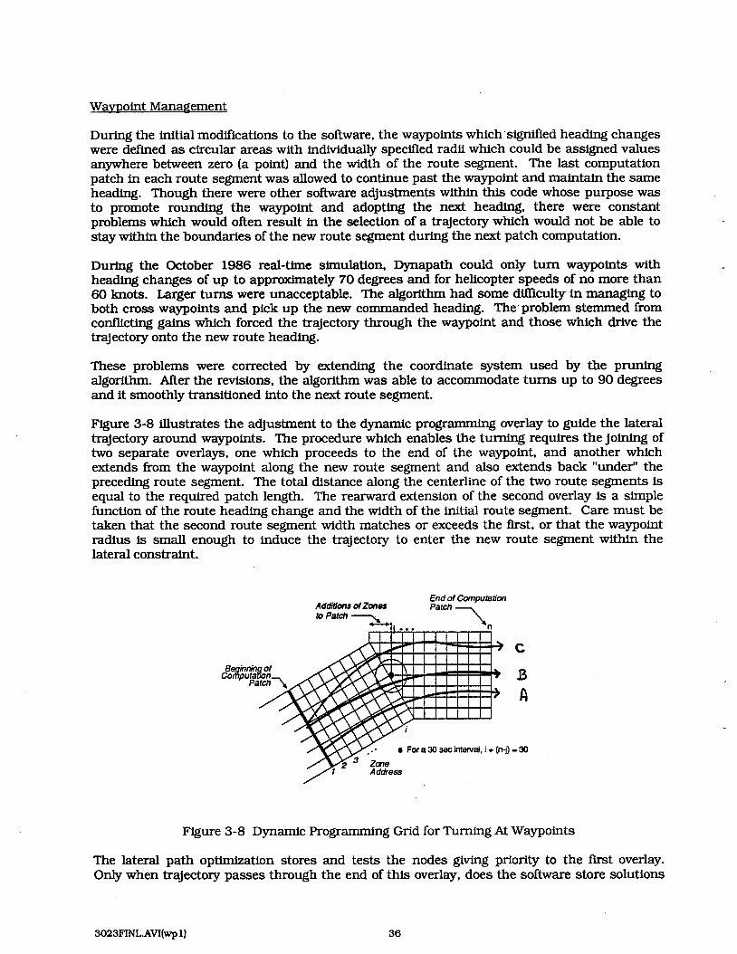
Figure 3-8 illustrates the adjustment to the dynamic programming overlay to guide the lateral trajectory around waypoints. The procedure which enables the turning requires the joining of two separate overlays, one which proceeds to the end of the waypoint, and another which extends from the waypoint along the new route segment and also extends back "under" the preceding route segment. The total distance along the centerline of the two route segments is equal to the required patch length. The rearward extension of the second overlay is a simple function of the route heading change and the width of the initial route segment. Care must be taken that the second route segment width matches or exceeds the first, or that the waypoint radius is small enough to induce the trajectory to enter the new route segment within the lateral constraint.

C

B A

For a 30 sec intecval, i + (n-j) = 30

Address F Figure 3-8 Dynamic Programming Grid for Turning At Waypoints

The lateral path optimization stores and tests the nodes giving priority to the first overlay. Only when trajectory passes through the end of this overlay, does the software store solutions

in the second overlay. Headings and performance costs in the second overlay are computed with respect to the new direction. All paths which are propagated to the end of the path are compared to find the lowest cost, or optimum. This technique rewards trajectories which take the "inside" of the turn since the distance is reduced. Trajectory A, for example is shorter than B or C and the total cost might be lower by virtue of having fewer nodes summed into the total cost. However, if the TF/TA ratio (a) is set to a high value, then trajectory B would have a lower accumulation of lateral cost, though it is longer. In either case the only way path C, which takes the "outside bend," would be of lower cost, is if the terrain elevation cost component is signfncantly lower than that of the others.

Cost Measure Modifications

During the course of integrating Dynapath into the real-time simulation environment, a considerable number of modincations were introduced which altered the pure Dynamic Programming nature of the software and forced it to adapt to a real-world environment. The TF/TA ratio was one of those modifications. It was observed that over most of a route segment, there was little reason to prefer the centerline of a route segment to any other area. By providing a slight penalty for headings which deviate from the route heading, sensible trajectories were found which would tend to fly parallel to the centerline, but maintain whatever lateral offset resulted from earlier maneuvers which avoided terrain obstacles. In fact, as Figure 3-9 shows, a TF/TA factor can generate senseless behavior. Trajectory A returns to the centerline for no apparent reason, thus requiring four maneuvers to avoid two obstacles while trajectory B maneuvers once to bypass both obstacles. As long as the DP tree generation procedure is capable of propagating branch trajectories from one side to the other of the route segment, then the TF/TA factor should not be assigned a large value.

The TF/TA factor can be useful. however, as the aircraft approaches a waypoint. By increasing the lateral deviation cost factor (a) as the trajectory nears a waypoint, the pruning algorithm promotes candidate paths which gravitate toward the centerline.

Waypoints are treated as circular areas which it is important to overfly. Thus, if a point is to be overflown, the waypoint radius is assigned a value of zero; if there is no major importance other than the desire to take up a new heading in the next route segment, the waypoint can be assigned a radius nearly equal to the width of the route segment. It then becomes unimportant to have any TF/TA ratio influencing trajectory segments which are no further from the centerline than the radius of the waypoint. Accordingly, the lateral path cost measure was modified to include a "deadband" in the lateral measure component of the cost computation. The increasing TF/TA and deadband regions are illustrated in Figure 3- 10.

The revised cost measure is:

where:

J hi 0 (XI di dB W i Vref gw

the cost measure terrain elevation value at cell i TF/TA ratio - a function of the distance to the next waypoint the lateral deviation from reference path the route segment deadband the trajectory heading the heading of the route segment the gain on heading error

(Eq. 3.4- 1)

Figure 3-9 Sample Lateral Paths Over a Patch

Deadband,

Area of Increasing

FmA 7

Figure 3-10 Sample DP Patch with a Deadband

A menu capability was instituted in Dynapath to simplify the program input processes. This technique allows for manipulation of all key program parameters, including the establishment of sets of waypoints for real-time simulation runs. Entire parameter sets can be easily stored and recalled as data files. Figures 3- 11 to 3-14 illustrate, in screen display format, the Dynapath parameters available to the user.

The parameter default settings are read from a data file, and the user can also write a configuration of settings onto a selected data file. The principal menu. Figure 3-1 1, displays the aircraft initial state, the performance limits to impose on Dynapath, the dynamic programming parameters which determine the tree generation and pruning characteristics, and also settings which enable/disable various display plotting features.

The user can also interactively select the terrain data base and direct the program to display other submenus. These submenus are shown in Figures 3-12 to 3-14 and include the designation of route segment, waypoint, and circular threat data.

The menu software has been delivered to NASA It is easily modified to accommodate new parametem and submenus. The current display configuration differs from what is shown in this report.

Terrain Offsets

The Dynapath optimization technique searches for the least cost trajectory of a point moving aver a digital terrain map. There is no direct accounting for the actual size of the aircraft nor for any clearance margins which may be necessary to compensate for errors and drift in the navigation system. A lateral clearance can be accounted for by passing a smoothing filter over the digital terrain map, but that poses a large data management problem (storing and reading several versions of the same map), and it also tends to reduce the flexibility of the software in a real-time environment.

To handle this dilemma, a real-time terrain "smearing" algorithm was introduced. This algorithm provides the lateral path generation algorithm with digital terrain smoothed data while it maintains the unfiltered terrain in computer memory. A kernel, typically 5x5 is placed over any terrain coordinate requested by the lateral path performance measure algorithm. The highest value within the kernel supplied as the reference terrain elevation. In a lateral path optimization cycle, this search is repeated approximately 50,000 times for 30 seconds of trajectory optimization.

The outcome of this simple process is quite dramatic. First, in the real-time simulations. trajectories which had been guided along the very edge of large walls, now maintain a comfortable offset. Secondly, the algorithm does not appreciably increase the computation time. In typical patch computation, which requires about 5 seconds, the overhead for searching with a 5x5 "smearing kernel is about 1/2 second. If a more extensive smearing algorithm were required to be implemented, the real-time requirements could be maintained by performing this process with a dedicated image processing board.

The benefit of this approach to handling terrain offsets is in its simplicity and versatility. In an operational flight environment, the navigation system would supply Dynapath with position uncertainty data. This could be used to apply to the smearing parameter. The lateral path algorithm would then fuse the filtered terrain data with on-board sensor information for path optimization.

INPUT>> DYNAPATH 4.3

* INITIAL STATE >

1 X WSlTlON (FT)

2 Y POSITION (FT)

3 Z POSITION (FT)

4 HEADING ANGLE (DEG)

5 PRESENT BANK CONTROL

6 PREVIOUS BANK CONTROL

7 PITCH (DEG)

8 PREVIOUS PITCH CONTROL

- FLIGHT LIMITS r

21 SET CLEARANCE ALT (FT)

22 VELOCITY (KNOB)

23 MAX BANK ANGLE (DEG)

24 MAX HEADING (DEG)

25 MIN HEADING (DEG)

26 MAX PITCH (DEG)

27 MIN PITCH (DEG)

40 TERRAIN FILE NAME: [-]dynl

TAU CORPORATION - TREE CONTROLS :,

10 NUMBER OF FORWARD ZONES

11 NUMBER OF DEVIATIONS

12 HORIZONTAL ZONE

13 FIRST ZONE

14 TIME TO SWITCH TREE SIZE

15 NEW TREE SUE

16 TIME UMlT FOR VERTICAL

17 UPDATE TIME

-PLOTTING: YES=1 /NOSO>

31 TRAPIX ENABLE

32 DRAW TREES

33 DRAW SET CLEARANCE

34 DRAW PRUNED NODES

35 DRAW SOLUTION

36 DRAW PATCH SEGMENTS

41 WAYPOINT MENU...

42 THREAT MENU...

Figure 3- 1 1 Dynapath Main Menu

INPUT >v ROUTE SEGMENT MENU TAU CORPORATlON

ROUTE WEIGHT PENALTY WAY POINT WEIGHT PENALTY SEGMENT FOR CROSSRANGE TRANSIT FOR HEADING AT

WlDTH DEVlATlON I E E WAYPOlNT 11: 21 : 31 : INGRESS ETC... 41 : 12: 22: 32: OPTlONAL 42:

1 n: 2n: 3n: 4n:

m-4 Il/ee

INPUT >w

Fgure 3- 12 Route Segment Menu

WAYPOINT MENU TAU CORPORATION

50 ROUTE SEGMENTS MENU... Dm-'2 11/88

1: NUMBER OF WAYPOINTS n

Figure 3- 13 Waypoint Menu

INPUT >>

xlQsma 10:

11:

12:

13:

THREAT MENU TAU CORPORATION

zlQmQN 30:

31 :

32:

33:

YlessmN 20:

21 :

22:

23:

RADlUS

40:

41 :

42:

43:

Figure 3- 14 Threat Menu

4 1

1 : NUMBER OF THREATS n

x-ms.mm Y-mmQN RADlUS rYeE 10: 20: 30: 40: 11:

In:

31 :

3n:

21 :

2n:

41 :

4n:

Path Reversals

During the October 1986 simulation, Dynapath frequently made major path decision changes which demanded a radical altering of the aircraft heading. These changes, or path reversals. caused the HUD display of the next several seconds of anticipated flight to be overwritten. Not only was the frequent change of the guidance data visually hard to follow, but it also caused the pilot to lack confidence in the algorithm. It can be extremely disturbing to a pilot who is anticipating one maneuver and then is being requested to change to another.

The control reversals did not usually result in signincant cost changes. The variations typically reflected that the algorithm discovered a slightly better opportunity than was apparent in the previous time interval. Since the function of Dynapath is to obtain optimal trajectories as determined by the TF/TA constraints of the flight, it is encouraged to seek even slight improvements.

One reason that control reversal frequently occurred during the simulation was due to the use of an abbreviated search path time, or length, (21 seconds). The search path length was kept at this value in order to keep the computation time at or below 6 seconds. However, the shorter the search distance, the more likely that solutions will occur which are unflyable.

In order for Dynapath to search far enough ahead to foresee dimcult terrain, the search process was revised to generate nodes at one second intervals in the near term and to expand the segment lengths for the most distant portions of the search process. The favorable effect of this measure on the performance of the algorithm is discussed in Section 3.5.

In addition to providing the algorithm an adequate search distance, a smooth trajectory prediction technique is guaranteed by '"pinning" each updated path data only onto the end of the previous solution data set. Each Dynapath computation is now initialized with the last state data which is expected to be sent to the HUD display.

This process proved to successful in subsequent simulations.

3.5 KEY PARAMETERS WHICH AFFECT THE SOLUTION PROCESS

The following is a list of the constraints and parameters of greatest significance to the Dynapath algorithm. Slight variations in the values selected for these items often have a large effect on the overall behavior of the algorithm in terms of run time and trajectory behavior. Much has been learned about these effects, yet the process of selecting parameters is not an intuitive one. In general, as more severe constraints are applied fewer trajectories are evaluated. This results in a restricted selection of possible paths for the vehicle.

Path Selection Parameters:

The number of nodes in each generation The look-ahead flight time (trajectory length) The estimated Dynapath patch computation time Grid space density (number of zones and divisions)

Performance Cost Parameters:

Route segment width The TF/TA ratio Lateral deadband Terrain elevation (2) gain

Smear factor Controls:

The gain on heading division from route azimuth Max/Min allowable heading division

Waypoint Radius Distance from waypoint for TF/TA gain modification

Helicopter Model Parameters:

Aircraft Velocity Max Climb/Descent Angles Max G-load Max Bank angle Intermediate bank angle

The effects of these parameters on performance are discussed below:

Path Selection Parameters

In addition to the effects of gains on the quality of the Dynapath trajectory generation, there are other parameters which have a direct effect upon the degree to which the algorithm propagates a variety of exploratory trajectories by which it is able to evaluate the least cost or 'best" path. The number of controls used and the aircraft turn and climb characteristics detennine.the number of possible path segments which may be created. Path segments are then pruned at intervals to eliminate multiple trajectories which have reached similar locations and have similar headings. The pruning process selects the least cost path for each "cell" or grid space.

However, if the grid spaces are very coarse, the pruning process may eliminate too many trajectories and curb the growth of path segments having the potential of passing through the narrow gaps or pathways through difficult terrain. By allowing a large number of intermediate trajectories to propagate, an excessive computational time requirement may impact real-time simulation performance.

A study was made of the trade-off between algorithm execution speed and trajectory quality over a particularly demanding segment of the NASA NOE terrain database. The NOE route calls for traversing several prism-shaped berms, each of which has either a notch or valley (complete cut). These passageways are laterally scattered as illustrated in Figure 3-15. The key parameters which affect the number of path segments are:

the number of Divisions or lateral cells; the number of Heading cells; the number of Trajectory Generations before pruning.

Figures 3-16 and 3-17 display the computation time required for a selection of divisions, headings, and trajectory generations. The fastest executing parameter selections tend to produce fairly crude trajectory paths, while the parameter selections which generate trajectories through every valley and notch require an unacceptable amount of computation time.

The best trades in speed of execution and a reasonable quality of trajectory can be found by using either 3 or 4 generations, 20 division cells, and 5 heading cells. Similar performance and speed of computation were obtained with 3 and 4 generations.

NOTCH WIDTH = 200' TYPICAL BERM

Figure 3- 15 NASA NOE Terrain Database Waypoint Set #6

+

Berm

No.

1

2

3

4

5

Berm

Height

(ft.1

600 ft.

200 ft.

400 ft.

200 ft.

300 ft.

Breadth

(ft.1

2000 ft.

1000 ft.

1500 ft.

1000 ft.

1000 ft.

Notch

Height

(ft.1

400 ft.

-

100 ft.

-

200 ft.

Notch Lateral Displacement

(ft.) from Center tine

600 ft.

- 600 ft.

600 ft.

- 6OOft.

600 ft.

No. of Generations = 4

Y - No. of Headings

650,

600,

h

400 - 5

4 6 8 10 12 14 16 18 amc4-f 11m

CPU (sec)

Figure 3- 16 performance A d y s i s Cost vs CPU NASA NOE Database Waypoint Set #6

C I

f t flies hwgh some nolahes

No. of Generations = 3

10 flies hmgh allnotches and some velkys

Yy 16 20

9 9 13

300 1 I I I I I I I I I 4 5 6 7 8 9 10 11 12 13

OENE3 .F 11/88 CPu ( s ~ c )

Figure 3- 17 Performance Analysis Cost vs CPU NASA NOE Database Waypoint Set #6

Performance Cost Parameters

The various gains which affect the trajectory generation process in Dynapath have subtle effects on the performance of the algorithm. The relationship of these gains cannot be readily observed. A simplified model was developed using the Lotus 1-2-3 spreadsheet program on an IBM-PC/AT system to further study these effects. A calibration of this model compares closely with actual Dynapath trajectories. The gains of particular concern are:

Heading Gain - The gain that penalizes the division from the nominal heading.

TF/TA Ratio - The penalty that is applied to the path when it departs from the route segment centerline.

Deadband - The allowable distance the trajectory can depart from the centerline before the lateral penalty begins to be applied.

Altitude Gain - This value is generally used to scale the altitude data into the same units used in the lateral measure.

Figures 3-18 and 3-19 illustrate the effect of these gains using this simple model. The curves of Figure 3-18 show the performance effects with respect to the trajectory which is required to fly through the first notch in Waypoint Set #6 of the TF/TA DMA Data Base (Figure 3-15). In Figure 3-18, the highest curves (A. and B) show the top-down and altitude profiles of the trajectory as it moves laterally 650 feet from the centerline, passes through the notch in the berm, and then returns to the centerline. Curve C shows the cumulative cost using the cost function of Equation 3.4-1. Curve D shows the cumulative cost using the same metric for a trajectory which, instead of diverting to the notch, flies directly over the 600-foot high berm. A s can be seen in the figure, the net cost for diverting to the notch is less than the cost of flying straight ahead (a desirable feature). This effect is for a TF/TA ratio of 0.1, and a deadband on the lateral offset of 400 feet. The notch is displaced 600-800 feet, and the trajectory diverts about 680 feet.

The degree to which it is worthwhile to divert an aircraft around an obstacle depends upon the tradeoff between maneuvering over to a lesser degree of obstruction and the amount of relief from climbing the maneuver affords. Figure 3-19 shows the performance trades using the same cost function and parameter settings, but with variations applied to:

the penalty for diverting (Curve A)

the height of the notch (Curve B)

The curves each show the relative cumulative cost of the maneuver compared to the cost incurred by flying directly over the 600-foot high berm. For example, in Curve A, maneuvers over to the notch which is 600 feet from the centerline are of lower relative cost than direct overflight of the berm provided the deadband which measures the onset of penalizing lateral maneuvers is set to a value greater than about 150 feet. The higher the deadband, the greater the cost reduction.

Similarly, Curve B shows the large payoff for maneuvering through deep notches, and the decline in reward as the notch height increases. For this curve, notches of height below 500 feet are worth maneuvering over and through with a deadband assigned at 400 feet.

This Cost Parameter model serves as a convenient tool for examining the effects of the different gains on the Dynapath algorithm.

20 40 60

INTEGRATKMI INTERVAL NUMBER

Figure 3- 18 Dynapath Performance

Heading Gain - 1 & Deadband Gain = 0.1

t ' V) 0 U +' r 0, .- e I5 .,- 0 t' c U

!! U U.

0 100 200 400 500 600 700

Notch 01- Deadband Value (ft)

Figure 3- 19 Dynapath Performance Summary

48

Helico~ter Model Parameters

The degree of helicopter maneuverability closely affects the performance of the Dynapath algorithm in several respects. The bank angle and aircraft velocity determine the horizontal curvature controls. If these knits are too severe with respect to the terrain, then the lateral path algorithm may, by default, force non-optimal trajectories over rough terrain. Such trajectories could require early climb onset to stay within the climb angle limits of the aircraft. As these climb/descent angles are limited, a point is reached where it is totally impractical to maintain true NOE flight.

The maximum G-loadings for the initiation of both climb and descent directly affect the ability of the helicopter to follow the terrain profile. If the G-load limit is overly restrained, then the response of the helicopter to high frequency terrain elevation changes is damped. The aircraft must either maintain a higher clearance margin or be flown more slowly.

A way to enhance the performance of Dynapath when trajectories are sought for a helicopter with restricted mobility is to vary the velocity as a function of terrain roughness and clearance altitude. Further, the climb and descent limits can generally be increased as the velocity is reduced. Thus in rough terrain, the radius of curvature can be reduced fourfold by halving the velocity. The result is a great increase in mobility around hazards. A preprocessing of the terrain can be performed to generate a velocity/terrain clearance map. This function would typically be performed by the mission planner.

A discussion of velocity variations within a patch computation occurs later in this report.

Path Generation Changes

Several modifications were made to the lateral path generation algorithms to enhance the quality of the local trajectory solutions within the computing time limits. Key changes are discussed below:

Variable Partition Intervals in the Dvnamic Programming Overlav. Larger lateral cells are generated near the extremes of the route segment and a reduced lateral cell size exists near the center of the route segment. The same variable concept is applied to the heading partitions where a larger number of choices exist for headings in the general direction of the route segment. This procedure is designed to balance bank angle and G-load capabilities of the helicopter model. The philosophy of this is that the run time is directly related to the number .

of cells used. The cells at the extremes are infrequently the lowest cost, since in all cases. both position and heading penalties are applied.

Dual Steps. In order to assure that Dynapath could compute patch lengths of adequate length in a reasonable time internal, a dual step size was instituted. With dual step sizes. Dynapath explores possible paths using 1 second time intervals to a certain length (usually about 50% of the patch length), and then evaluates the remainder of the patch with a larger step size, usually 2 seconds. The controls and maneuvering characteristics are adjusted accordingly.

Figure 3-20 shows the computation time sensitivity to the time along the patch computation at which the change from one step size to another takes place. Obviously, the earlier the change, the few total path options are examined. However, in all cases, Dynapath looks along the same patch time interval. In this figure, the time interval is 30 seconds. For 100 sample cases, the mean computation time associated with a step change at 20 seconds was 4.8 seconds, with the longest time requirement of the 100 samples requiring 9.0 seconds.

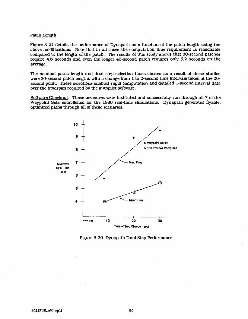
Patch Length

Figure 3-21 details the performance of Dynapath as a function of the patch length using the above modifications. Note that in all cases the computation time requirement is reasonable compared to the length of the patch. The results of this study shows that 30-second patches require 4.6 seconds and even the longer 40-second patch requires only 5.2 seconds on the average.

The nominal patch length and dual step selection times chosen as a result of these studies were 30-second patch lengths with a change from 1 to 2-second time intervals taken at the 20- second point. These selections enabled rapid computation and detailed 1-second interval data over the timespan required by the autopilot software.

Software Checkout. These measures were instituted and successfully run through all 7 of the Waypoint Sets established for the 1986 real-time simulations. Dynapath generated flyable, optimized paths through all of these scenarios.

10 --

9 -.

8 --

Microvax -- CPU Time

+ / / 0 waywint s n n / o 100 Patches Computed

Time of Step Change (sec)

Figure 3-20 Dynapath Dual Step Performance

o Waypoint Set #7 o 100 (+25) Patches Computed

Miimvax CPU T i e 7

*\-- Mean Time

I I I 302b2 11B8 20 30 40

Patch Length (sec) .

Figure 3-2 1 Patch Length Compute Time Sensitivity

3.6 ENHANCEMENTS NEEDED FOR DYNAPATH FLIGHT TESTING

There are several modifications which are necessary to transition the Dynapath software from the simulation environment to flight evaluation. Figure 3-22 diagrams the necessary Dynapath interfaces in a flight environment. Shown is a requirement for the pilot to be able to activate and deactivate the algorithm; elements such as known threat and exposure data and blended sensor information influence the path generation: and there are other factors which must be applied to integrate the sensor system with the Dynapath trajectory information to provide the pilot with the most current flight cues. These matters are discussed below:

Enacting and Disabling the D m a t h Algorithm

The enable and disable intedace between the pilot and the Dynapath algorithm has several real-time considerations. There is a latency between when the algorithm begins its calculations and when it can deliver trajectory information. Currently, with a 1 MIP MicroVAX I1 computer, 6 seconds is a typical time for 30 seconds of commanded flight. Even when the pilot has disabled the applicatioh of the Dynapath algorithm, the software should continue to operate in a passive mode, computing the trajectory to be flown. After each computation cycle the software should test to determine if the pilot has enabled the application of the algorithm. If so, it can proceed to send the results to the HUD or autopilot. If not, then it can recycle. Thus, the latency between when the pilot summons the algorithm and the time when results are available is anywhere between zero and the full computation interval.

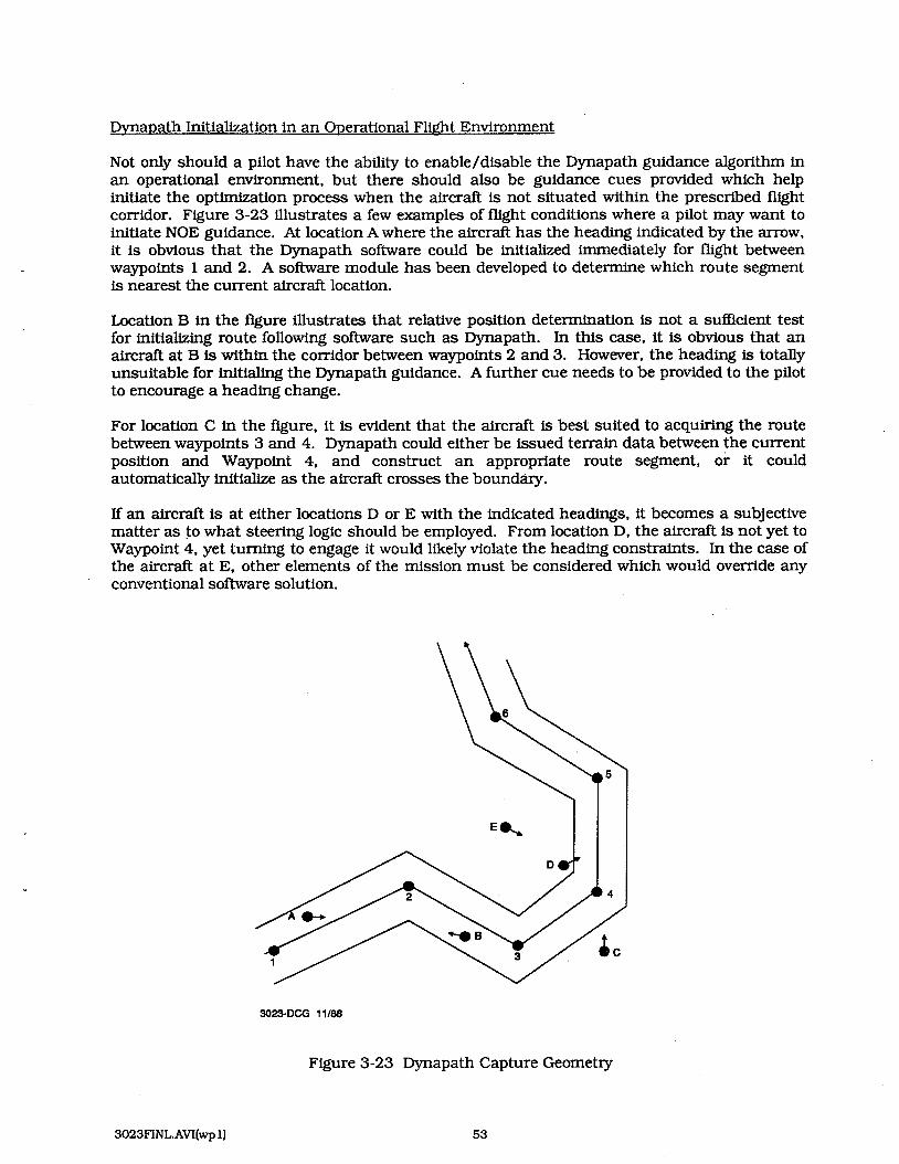
Dvna~ath Initialization in an O~erational Flight Environment

Not only should a pilot have the ability to enable/disable the Dynapath guidance algorithm in an operational environment, but there should also be guidance cues provided which help initiate the optimization process when the aircraft is not situated within the prescribed flight corridor. Figure 3-23 illustrates a few examples of flight conditions where a pilot may want to initiate NOE guidance. At location A where the aircraft has the heading indicated by the arrow, it is obvious that the Dynapath software could be initialized immediately for flight between waypoints 1 and 2. A software module has been developed to determine which route segment is nearest the current aircraft location.

Location B in the figure illustrates that relative position determination is not a sufficient test for initialking route following software such as Dynapath. In this case, it is obvious that an aircraft at B is within the corridor between waypoints 2 and 3. However, the headmg is totally unsuitable for initialing the Dynapath guidance. A further cue needs to be provided to the pilot to encourage a heading change.

For location C in the figure, it is evident that the aircraft is best suited to acquiring the route between waypoints 3 and 4. Dynapath could either be issued terrain data between the current position and Waypoint 4, and construct an appropriate route segment, or it could automatically initialize as the aircraft crosses the boundary.

If an aircraft is at either locations D or E with the indicated headings, it becomes a subjective matter as to what steering logic should be employed. From location D, the aircraft is not yet to Waypoint 4, yet turning to engage it would likely violate the heading constraints. In the case of the aircraft at E, other elements of the mission must be considered which would override any

' conventional software solution.

a23-DCG 11/88

Figure 3-23 Dynapath Capture Geometry

It is clear that a purely automated technique for initializing NOE guidance is impractical. The pilot should be given cues which help him to decide a course of action. An appropriate HDD for this system would display the current aircraft position. the waypoints. and the corridors. The pilot should then be able to point, via cursor control or other means, at the intended next waypoint. It then becomes an easy task for software to generate simple maneuvering cues to acquire the route segment (see Reference 2). or a new corridor can be constructed to the waypoint.

Use of Other Than Terrain Elevation in the Dvnauath Cost Function

There are several other terrain oriented considerations which may be significant in determining the optimum flyable path in the NOE environment. The implementation of Dynapath for the purposes of this study has been one of searching for the lowest terrain elevation, or "valley- seeking." Though it is often the best thing in general to do when attempting to avoid being either visually spotted or sighted on radar. this optimization parameter does not always provide minimum exposure. The algorithm is capable of generating high exposure by flying over steep ledges where the lateral path generation algorithm directs the aircraft to low terrain elevations. It is generally better to hug the sides of steep terrain. This characteristic can be attained in Dynapath by comparing the terrain elevation measure with that of the prior node of obtain the gradient, or slope. The cost function can be modified to penalize trajectories which are required to climb or dive at rates in excess of the operating parameters of the aircraft.

Another way to avoid exposure is to fly in areas of high clutter or low population density. The digital terrain maps (DTED) provide no indications of such masking aids as vegetation or of the probability of people or sensors being situated. If this information is made available via other sources such as the Level I1 DMA digital maps, the cost function of Dynapath can be modified ,

to penalize high exposure and reduce the cost of flying over low probable exposure areas.

In a peace-time role, the application of similar cultural feature data can be employed to avoid power lines, antennas, hospitals, stadiums, schools, and other facilities. The Dynapath algorithm can also be used to modify routes flown at intermediate altitudes to generate low noise profile routes in populated areas and to monitor the selection of emergency landing areas.

The degree of maneuvering should also be modlCied to be a function of the clearance altitude. It is wasteful, with regard to energy consumption and ride-quality, to endure highly varying turns and climbs/descents at aircraft altitudes which are not in the NOE or near NOE environment.

Route Segment Geometry

A flexible interface is needed which converts mission planning data to usable Dynapath route segments. The mission planning system is principally a generator of waypoints. Other information is required to define the waypoint radii. Perhaps commanded waypoints require a small radius while intermediate waypoints which are intended to define the overall route could be a function of the separation of the points or merely have a standard value. .

The waypoints, with defined radii, should then serve to define the route segments used in the Dynapath navigation software. Figure 3-24 illustrates the aspects of this route segment geometry. Note that the deadbands can be defined by the waypoint radii, and might then vary along the route segment when different radii are employed. Likewise, the distance separating the waypoints. and their radii should serve to define the width of the route segments. By applying both maximum and minimum acceptable values, and otherwise applying a linear relationship between length and width, the overall route geometry can be easily defined.

Dynapath currently uses only fixed limits for the deadbands and route segment boundaries, but could be easily modified to conform to variable values.

Figure 3-24 Dynapath Route Segment Geometry

Energy Management Flight Profiles

During the course of the contract, the Dynapath software was evaluated in a constant velocity mode. It was assumed for the real-time simulations, that sufficient power was available for the aircraft to maintain the flight profile commanded by the algorithm. A s long as there is sufficient excess power, and this power can be applied rapidly, then the vehicle should be able to maintain the commanded flight velocity.

In an actual flight environment, winds, power limitations, and other factors may adversely affect the ability to maintain a constant velocity. The Dynapath algorithm must compensate for velocity variations and even should suggest or command velocities appropriate to the local conditions. There are occasions where either a velocity change is highly desirable or inadequate power exists for maintaining velocity over the commanded maneuver.

For example, in an unchecked mode. Dynapath may determine lateral and verticd trajectories which are flyable, but when coupled, the combination of lateral and vertical accelerations to perform the maneuver at the nominal velocity may exceed the available power of the aircraft. By slowing down, the commanded lateral turn radius might be maintained, thus avoiding detected hazards, and sufficient power might then be made available for the required climb angle.

There are other circumstances where the power available to the aircraft may be adequate, but that a velocity change is suitable. A minor obstruction might be most appropriately dealt with by trading kinetic energy for potential. This is a mode of flight at constant energy, where

velocity is temporarily exchanged for altitude during brief climbs or zooms, and the engine power is not changed. The velocity is resumed during the descent on the "backside" of the obstacle.

In yet another scenario, it may be appropriate to vary both velocity and the set clearance altitude as a function of terrain roughness or aircraft exposure. In a highly cluttered environment, it may be best to fly as close as possible to the vegetation, thus necessitating very slow flight. Where there is no appreciable masking, the minimum exposure time is obtained by flying at the maximum safe velocity in a "high as you dare" clearance over the ground.

It is feasible for Dynapath to be adapted to both command and apply variable velocity. By prestoring maneuvering performance data and sets of turn radii for different velocities, the Dynamic Programming algorithms need only slight modification to be able to apply velocity variations. The equations below solve for the power required to maneuver the aircraft.

The energy state E for the helicopter can be described as:

where: E is the energy Wt is the aircraft weight V is the true airspeed g is force of gravity h is the aircraft altitude

(Eq. 3.6- 1)

The energy of the aircraft can be increased by applying additional engine power, if is it is avaflable. Power is the rate of change of energy:

Power = dE/dt (Eq. 3.6-2)

The available excess power can be stored as a function of weight, altitude. and velocity. Figure 3-25 (Reference 7) illustrates the power available and power required for a typical helicopter. The difference between these two values is excess power. For climbs, power must be applied at the rate of:

where:

Px is the excess power required y is the flight path angle

Thus, if no velocity change is desired:

is the relation between climb angle and power required. Thus when coupled maneuvers are tested and found to demand excess power, the velocity reduction can be computed which correspondingly reduces the horizontal acceleration and allows power for climb.

By assuming a time dependent velocity profile which is a rough approximation of what is anticipated, the lateral path algorithm of Dynapath can be employed without major

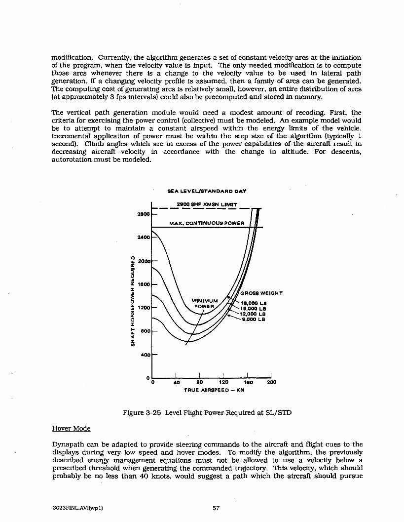
modification. Currently, the algorithm generates a set of constant velocity arcs at the initiation of the program, when the velocity value is input. The only needed modification is to compute those arcs whenever there is a change to the velocity value to be used in lateral path generation. If a changing velocity profile is assumed. then a family of arcs can be generated. The computing cost of generating arcs is relatively small, however, an entire distribution of arcs (at approximately 3 fps intervals) could also be precomputed and stored in memory.

The vertical path generation module would need a modest amount of receding. First, the criteria for exercising the power control (collective) must be modeled. An example model would be to attempt to maintain a constant airspeed within the energy limits of the vehicle. Incremental application of power must be within the step size of the algorithm (typically 1 second). Climb angles which are in excess of the power capabilities of the aircraft result in decreasing aircraft velocity in accordance with the change in altitude. For descents. autorotation must be modeled.

SEA LEVEUSTANDARO DAY

I 2900 SHP XMSN LIMIT L--------

2800 - MAX. CONRNUOUS POWER

TRUE AIRSPEED - KN

Figure 3-25 Level Flight Power Required at SL/STD

Hover Mode

Dynapath can be adapted to provide steering commands to the aircraft and flight cues to the displays during very low speed and hover modes. To modlfy the algorithm, the previously described energy management equations must not be allowed to use a velocity below a prescribed threshold when generating the commanded trajectory. This velocity, which should probably be no less than 40 knots, would suggest a path which the aircraft should pursue

when it accelerates out of the hover or very slow flight mode. The selected velocity must be adequate to provide the HUD with a reasonable path in the sky to follow. In this flight mode, a path in the sky display would be more useful than a flight director mode which only cues the next maneuver to make.

The process used for initializing successive Dynapath computation cycles would be driven by the INS. As the aircraft maintains a near hover, the HUD display would maintain error corrections. As the aircraft position/velocity maneuvers beyond prescribed limits, the software would estimate a new commanded trajectory using the same principles associated with initializing the algorithm.

4.0 DMA DIGITAL MAP INTERFACE

It is important both for real-time NOE flight path management (Dynapath) and for mission planning to access DMA data and use it expediently. Four level I Digital Terrain Elevation Data (DTED) sets were merged to present a map of the San Francisco Bay Area and were then loaded and displayed on the TAU Trapix image processor. The Bay Area was selected for its fammuity.

A series of test Dynapath trajectories were then attempted using this data. The photos accompanying this report illustrate the results of the effort.

Figure 4- 1 is an illustration of the northern 75% of the terrain map as displayed on the image processor using a pseudo-color lookup table which amplify the details of the terrain elevation. All processed pixels in the display which had sea level elevations were painted blue, hence the apparent body of water in the upper right (delta area) which is not accurately represented. Note that lower elevations were coded in varying shades of green, while the higher elevations were tinted in shades of reddish brown. The use of this color table tended to highlight the ravines and valleys fn the area.

The photos in Figures 4-2 to 4-9 exhibit the details of using Dynapath to command an NOE flight from Marin County past Angel Island and on to a randomly selected location in San Francisco.

The trajectory is both constrained by the Dynapath geometric settings (waypoints and route segment widths) and weighting parameters (TF/TA ratio, etc .I. ~dditionall~. the maneuverability and ride quality settings for the flight affect the derived path. The key parameters settings for these exercises are similar to those used in the real-time simulations. These values are:

Bank Angle 17 deg. G Loads -.25 to +.25 Climb Angle 23 deg. Descent Angle -20 deg. Aircraft Velocity 60 kts

In Figure 4-2, a 30-second trajectory patch is constructed which rounds the h g e l Island - waypoint. Note that the TF/TA weights are such that the algorithm prefers flight over water and until it must cross the island. The route segments are shown as longer rectangles in this illustration.

Figure 4-3 demonstrates the computational explosion associated with the variety of choices for one of the ffnal 30-second Dynapath patches while enroute to the destination. The selected trajectory steers as near as possible to the center, yet avoids the hills.

Figure 4-4 displays the trajectory solution for the entire route including overflight of the destination (WP4). Note the reasonable NOE behavior throughout in commanding the aircraft to seek terrain which is as low as possible yet also forcing the aircraft to cross the waypoint constraints.

Figures 4-5 and 4-6 illustrate a second exercise of Dynapath in a mountainous region near the San Francisco peninsula. The area is the Diablo Mountain Range and includes Mt. Hamilton (elevation 4200 feet). A trajectory is determined for a helicopter flight along one route segment through this area and through a waypoint. In Figure 4-5, the Dynapath has commanded the

helicopter into a valley, shown in green, and has generated a large number of candidate trajectories over a 30-second patch. The pink line indicates the selection chosen from the candidates.

Figure 4-6 is a similar example taken 30 seconds later in the trajectory. Note the commanded route continues to seek the valley. The path selected from the candidates gently rounds the waypoint and takes up the new desired heading.

ORIGINAL PAGE COLOR PHOTOGRAPH

Figure 4- 1 Compressed Digital Map San Francisco (North)

. - -!< ; L.. - . . < , <:i --- ; 7'- --:. ;+ - .

*.- . - h' V." .: .=>* 1 Gii*3

, , . - . :-,

, . - - . \, - " . L % ~

- .. , . --& - > , Jj - ., , .--.-

I-. a;. -:- ::

I,. . - ? . 1

&

Figure 4-2 Dynapath Trajectory Rounding the Angel Island Waypoint

ORIG tNAL PAGE COLOR PHOTOGRAPH

Figure 4-3 Choices of Dynapath Trajectories through San Francisco

E 4

Figure 4-4 Dynapath Trajectory NOE Flight Starting in Marin County

ORIGINAL PAGE COLOR PHOTOGRAPH

Figure 4-5 Dynapath NOE Trajectory in Mountainous Terrain

Figure 4-6 Rounding a Waypoint in Mountainous Terrain

5.0 CONCLUSION

This project has served to further develop automatic guidance techniques to be implemented in an engineering prototype for Nap-of-the-Earth (NOE) flight. With the advent of onboard digital map technology, these automatic guidance techniques make the map truly useful to the pilot while affording acceptable workload levels. The guidance techniques integrate sensed information on obstacles, power lines, etc., with digital terrain elevation maps to produce safe low-altitude flight corridors.

Such an integrated digital map/optimal NOE guidance system can revolutionize low-level helicopter operational performance and its impact on crew workload. The work performed under this SBIR contract will greatly enhance options for application of these automated guidance techniques in both military and civilian arenas. The military applications relate directly to Nap-of-the-Earth flight, including threat avoidance. Automatic guidance in this military application is virtually a necessity, a s has been recognized by several of the contractors establishing approaches to meet the potential LHX requirements.

There are numerous civilian applications as well, such as in low-altitude search and rescue (emergency medical services), in commercial localized emergency re-routing as well as in minimizing noise profiles in urban environments.

From the above. the program is of direct relevance to NASA as part of its long standing responsibility for advancing the operational utility of rotorcraft in both civil and military missions.

This contract has resulted in the following accomplishments:

Significant enhancements have been made to the technology of automated guidance in the NOE environment.

Real-time simulations of this flight mode have been successfully performed.

A commercial automated mission planning product has been developed to support routing helicopters in the NOE environment.

In the role of follow-on efforts, TAU has initiated conversations with several airframers including Boeing-Vertol and Sikorsky on the potential integration of elements of this effort into their advanced technology efforts.

As a result of these advancements, it is clear that automated aircraft guidance is not only possible, it is an eventuality.

REFERENCES

Pekelsma, N., et al, "Autonomous Flight and Remote Site Landing Guidance Research for Helicopters," Contract NAS 2- 12 180. TAU Corporation, August 1987.

Murphy. W. J.. et al, 'Tactical Flight Management Exploratory Development Program. McDonnell Aircraft Co., AWFAL/TR-84-3023, April 1984.

Denton, R V., et al, 'TF/TAAlgorithrn Study." AFWAL-TR-85-3007, TAU Corporation, May 85.

Denton, R V., et al, "Guidance Automation for Nap-of-the-Earth Flight," 7th Digital Avionics Systems Conference, October 1986.

Denton, R V., Jones, J. E.. and Denaro, R P., "Use of the DMA Digital Terrain Elevation for Flight Trajectory Generation," AGARD Lecture Series No. 122. March 1983.

Saunders, G. H., Dvnarnics of Helico~ter Flight, Wiley & Sons. Inc., 1975.

Stepniewski, W. Z., and Keys, C, N.. Rotarv-Wing Aerodynamics, Dover Publications, 1984.

"~e l i co~ te r Guidance and Control Systems for Battlefield Support," AGARD Conference Proceedings No. 359, May 1984.

NASA Nalml k m u t c s a M

Report Documentation Page Space Admmtslratm

Optimal Guidance with Obstacle Avoidance for Nap-of-the-Earth Flight

1. Report No. 1 2. Government Accession No.

NASA CR- 1775 15

4. Title and Subtitle

I December 1988 I

3. Recipient's Catalog No.

5. Report Date

6. Performing Organization Code c I Nicholas J. Pekelsma I I

I

10. Work Unit No.

7. Author(s1

9. Performing Organization Name and Address

Tau Corporation 485 Alberto Way, Bldg. D Los Gatos, CA 95030

8. Performing Organization Report No.

12. Sponsoring Agency Name and Address ,

Ames Research Center MS 210-9 Moffett Field, CA 94035

11. Contract or Grant No.

13. Type of Report and Period Covered

Contractor Report 14. Sponsoring Agency Code

I

15. Supplementary Notes

Point of Contact: David N. Warner, Jr., Ames Research Center, MS 210-9, Moffett Field, CA 94035

1 16. Abstract I

This report is on the development of automatic guidance for helicopter Nap-of-the-Earth (NOE) and near-NOE flight. It deals with algorithm refinements relating to automated real-time flight path planning and to mission planning. With regard to path planning, it relates rotorcraft trajectory charac- teristics to the NOE computation scheme and addresses real-time computing issues and both ride qual- ity issues and pilot-vehicle interfaces. The automated mission planning algorithm refinements include route optimization, automatic waypoint generation, interactive applications, and provisions for inte- grating the results into the real-time path planning software.

A microcomputer based mission planning workstation was developed and is described in this report. Further, the application of Defense Mapping Agency (DMA) digital terrain to both the mission planning workstation and to automatic guidance is both discussed and illustrated.

NASA FORM 1626 OCT 86 For sale by the National Technical Information Service, Springfield, Virginia 22161

17. Key Words (Suggested by Author(s))

NOE flight, Mission management Flightpath planning Obstacle avoidance

18. Distribution Statement

Unclassified-Unlimited

Subject Category - 08

Report Documentation Page

1. Report NO. 1 2. Government Accession NO. 3. Recipient's Catalog No.

NASA CR-177515 I I I Optimal Guidance with Obstacle Avoidance for Nap-of-the-Earth might

I

I December 1988 I 4. Title and Subtitle

6. Performing Organization Code , 5. Report Date

I Nicholas J. Pekelsma I I I

10. Work Unit No. 1

7. Authork)

9. Performing Organization Name and Address

8. Performing Organization Report No.

Tau Carporation 485 Alberto Way, Bldg. D Los Gatos, CA 95030

12. Sponsoring Agency Name and Address ,

Ames Research Center MS 210-9 Moffett Field, CA 94035

11. Contract or Grant No.

13. Type of Report and Period Covered

I Contractor Report I 14. Sponsoring Agency Code c

I

15. Supplementary Notes

Point of Contact: David N. Warner, Jr., Ames Research Center, MS 210-9, Moffett Field, CA 94035

16. Abstract

n the development of automatic guidanc helicopter Nap-of-the-Earth @JOE) and If deals with algorithm refinements ng to automated real-time flight path ssion planning. With regard to path planning, it relates rotorcraft trajectory charac-

teristics to the NOE computation scheme and addresses real-time computing issues and both ride qual- ity issues and pilot-vehicle interfaces. The automated mission planning algorithm refinements include route optimization, automatic waypoint generation, interactive applications, and provisions for inte- grating the results into the real-time path planning software.

A microcomputer based mission planning workstation was developed and is d e s c r i b e d m urther, the application of Defense Mapping Agency (DMA) digital terrain to both the mission

planning workstation and to automatic guidance is both discussed and illustrated.

17. Key Words (Suggested by Author(s))

NOE flight, Mission management Flightpath planning Obstacle avoidance

NASA FORM 1626 OCT 86 For sale by the National Technical Information Service. Sprinafield. Virginia 2216 1

18. Distribution Statement

Unclassified-Unlimited

Subject Category - 08

22. Price

A04 21. No. of pages

70 19. Security Classif. (of this report)

Unclassified 20. Security Classif. (of this page)

Unclassified