optimal groundwater remediation - the university of … · optimal groundwater remediation advanced...
TRANSCRIPT

Optimal Groundwater
Remediation
Advanced Chemical Engineering Design
Dr. Miguel Bagajewicz
University of Oklahoma March 14, 2008
Taren Blue, Laura Place

Executive Summary
This report is an exercise in the use of computational fluid dynamics and mathematical modeling to analyze the remediation process of groundwater. The purpose of this model is to minimize contaminants in an aquifer while minimizing cost. The mathematical model involves differing well configurations, pumping rates, and the use of fluid flow characteristics to evaluate the concentration profiles in the aquifer. This model builds on previous two dimensional models by adding simulations in Fluent flow simulation software in order to create a three dimensional model, and by investigating dynamic optimization through changing well configuration with time. The geometry of a 2000 m3 aquifer was drawn into Gambit, Fluent’s geometry software. This was imported into Fluent and boundary conditions were named for inlets and outlets of the aquifer. Fluid flow simulations were run. The velocities were analyzed at different points throughout the aquifer. Using the velocities in the contamination volume, a mathematical model was developed for the calculation of the contaminant concentration at points throughout the aquifer with time. The remediation time for each geometry and pumping rate was determined based on when the concentration of contamination within the aquifer dropped below the desired level. Well configuration was found to have a very large effect on flow patterns within the contamination plume. Seven well configurations were used in the analysis of flow profiles. Seven flow rates were used in each of the well scenarios. Remediation time was seen to be highly dependent upon flow rate. In some portions of the plume where the velocity of the water was at a maximum, the concentration profile was seen to behave as a step function. Cost analysis was performed for each of the evaluated scenarios. The cost was based on fixed initial and continuous costs, and variable operating costs. The biggest factors affecting cost were then the number of wells and overall remediation time. After this initial study was performed a refined fluid flow model was created. A more realistic geometry of an 8,000 m3 aquifer was created in Gambit and, again, imported into Fluent where inlet and outlet boundary conditions were defined. Simulations were run and the velocity data was imported into excel for analysis. Three different initial contamination plumes were explored in this study. In order to more effectively clean the differing plumes, unique pumping schemes were designed and varied with time. The total flow rate into and out of the aquifer was held constant throughout the entire remediation process. Each simulation was examined individually and as part of the dynamic model. Then, final concentrations were compared to investigate the most efficient pumping scheme. It was found that pumping scheme optimization is highly dependent upon the initial contamination profile. It was also found that this method can effectively model a dynamic pumping optimization scheme and can produce concentrations lower than those achievable with constant pumping configuration.

Table of Contents Introduction .................................................................................................................................................. 4
Options for Lowering Contaminant Concentrations ..................................................................................... 7
Industrial Practices and Current Research .................................................................................................. 10
Optimization ............................................................................................................................................... 11
Uncertainties and Problems with Remediation ...................................................................................... 11
Previously Developed Models................................................................................................................. 12
Fluid Flow Analysis ...................................................................................................................................... 14
Initial Fluid Flow Approach ..................................................................................................................... 14
Gambit................................................................................................................................................. 14
Fluent ..................................................................................................... Error! Bookmark not defined.
Initial Fluid Flow Simulations .............................................................................................................. 21
Concentration Profiles ........................................................................................................................ 26
Results and Discussion ........................................................................................................................ 30
Economics ........................................................................................................................................... 45
Secondary Fluid Flow Approach .............................................................................................................. 48
Gambit................................................................................................................................................. 49
Initial Plume Profiles ........................................................................................................................... 50
Pumping Strategies ............................................................................................................................. 51
Secondary Fluid Flow Simulations ...................................................................................................... 53
Fluent ..................................................................................................... Error! Bookmark not defined.
Construction of Concentration Profiles from Fluent Data .................................................................. 62
Results and Discussion ........................................................................................................................ 63
Further Studies and Future Work ............................................................................................................... 67
Conclusions ................................................................................................................................................. 68
Works Cited ................................................................................................................................................. 69

Introduction
Groundwater remediation involves the removal of contaminants from a water supply. Groundwater
contamination can generally be a result of agricultural or industrial processes (Hanford Site). Major
sources of contamination can be storage tanks, septic systems, landfills, hazardous waste sites, and road
salts and other chemicals (The Groundwater Foundation). Contaminants can include organic and
inorganic compounds, microorganisms, disinfection byproducts, disinfectants, and radionuclides.
Groundwater can also be contaminated with volatile organic compounds, or VOCs. According to the
National Water-Quality Assessment Program, in the United States, trihalomethanes and solvents were
the most frequently detected VOC groups.
In the United States, the contamination by some chemicals can be specific to certain regions of the
nation. For example, arsenic can be seen to be concentrated in areas in and around large cities.
Figure 1: Arsenic Contamination in the United States
Other than the United States, arsenic contamination is a large problem in countries including Mexico,
England, Chili, Argentina, Poland, Mongolia, Japan, Taiwan, Nepal, Bangladesh, and Vietnam. Nitrates in
the United States are observed to be concentrated in areas that have large farming areas. This can be
seen in figure 2.

Figure 2: Nitrate Contamination in the United States
This is due to the widespread use of fertilizers in agricultural practices. Other areas where nitrates are a
problem are Latin America, west, south and east Asia, north Africa, and other developing countries.
Heavy metals and minerals, the problems associated with “hard” water, are seen to be mostly
concentrated in the Midwest and eastern United States, as seen in figure 3.
Figure 3: Hard Water in the United States
VOCs (volatile organic compounds) are a common problem in many areas because they come from
many paints, varnishes, solvents and cleaners. The problem areas exist in large cities because these

particular chemicals come from industrial processes. The profile for VOC contamination in the United
States is shown in figure 4.
Figure 4: VOC Contamination in the United States
The major driving force behind the need for groundwater remediation is the adverse effects
contaminants have on the public. The following table outlines some of the common groundwater
contaminants and their adverse affects on health.

Compound Potential Health Affects Sources of Contamination
Benzene Known Carcinogen Discharge from factories, leaching from gas storage tanks and landfills
†,††
Vinyl Chloride Known Carcinogen Leaching from PVC pipes, discharge from plastic factories
†,††
Arsenic
Skin damage or problems with circulatory systems, and may have increased risk of getting cancer
Erosion of natural deposits, runoff from orchards, runoff from glass & electronicsproduction wastes
††
Copper Gastrointestinal distress, liver or kidney damage, and more
Corrosion of pipes and household plumbing systems, erosion of natural deposits
††
Lead
Delays in physical and mental development in children, possible deficits in attention span and learning disabilities. Adults can experience kidney problems or high blood pressure
Corrosion of pipes and household plumbing systems, erosion of natural deposits
††
Mercury Kidney damage
Erosion of natural deposits, discharge from refineries and factories, runoff from landfills and crop lands.
††
Trihalomethanes Liver, kidney or central nervous system problems, increased risk of cancer Biproduct of drinking water disinfection
††, †††
Nitrate
In infants, could cause illness or death; characterized by shortness of breath or blue-baby syndrome.
Runoff from fertilizer, leaching from septic tanks, sewage, and erosion of natural deposits.
††
Table 1: Contaminants and Health Effects
Because of their clear adverse effects on the community, these types of contaminants need to be
removed from polluted sites.
Options for Lowering Contaminant Concentrations Two very general options exist for lowering the concentration level of undesirable compounds found in
groundwater. They are dilution and treatment. In previous years, dilution was used to lower
contamination concentration because it is much less expensive than treatment of the contamination.
The problem with dilution is that it does not solve the problem but merely pushes the contamination
volume, or the plume, away from the original contamination site. Many of the current conventional
methods for treatment involve a pump-treat-inject (PTI) method. This consists of pumping water from
an aquifer, treating the water for contamination, and re-injecting clean water back into the aquifer. A
general PTI schematic is shown in Figure 5.

Figure 5: Pump-Treat-Inject Method
In the pump-treat-inject method, both injection and extraction wells are required. The number of
both types may be varied. Figure 6 shows the use of several well configurations involving no
injection or extraction wells to multiple injection and multiple extraction wells.
Figure 6: Depiction of PTI vs Dilution Only
In Figure 6, the darker gray represents higher contamination and the white represents the lowest
contamination. From Figure 6, case 2, we can see the affects of dilution only. It is clear from the large
white portion toward the center of the plume and the darker gray outer rings that the contamination is
only being pushed and the problem is not being resolved. In case 1 only extraction is being used and it

can be observed that the aquifer is being cleaned near the well sites but remains highly contaminated
away from the extraction. It is clear that a treatment method is necessary for resolving contamination
issues.
Some methods for purifying groundwater are use of membranes, distillation, reverse osmosis, liquid-
liquid extraction, ion exchange chromatography, and point of service treatments such as household
filters. Koch has developed membrane bioreactors for the treatment of water. A chart of some possible
water treatments and the contaminants they remove is given in Table 2.
Table 2: List of Treatments and Contaminants Removed
It can be seen in this table that distillation and reverse osmosis are two of the methods with the widest
range of applications for removing contamination. In the United States, the standards for the maximum
allowable concentrations of such contaminants in groundwater are set by the Environmental Protection
Treatment Method Iron b
acte
ria
Bacte
ria
Gia
rdia
& C
rypto
sporidiu
m C
ysts
Hard
Wate
r, C
alc
ium
, M
agnesiu
m
Ars
enic
Asbesto
s
Chlo
rine
Copper
Flu
oride
Iron a
nd M
anganese
Merc
ury
Lead
Nitra
tes
Oth
er
Inorg
anic
s
Dis
infe
ction B
ypro
ducts
MT
BE
Pesticid
es, H
erb
icid
es &
Insecticid
es
VO
C
Oth
er
Org
anic
Com
pounds
Chlorination x x x
Water Softener x / / /*
Ion Exchange Resin / / / / / / / / / / / / / / / /
Magnetic Conditioning
Whole House Sediment Filter x
Whole House GAC Filter / / / / / /
Ozonation Device x x x /
Manganese Greensand Oxidization Filter / x x
Distillation x x x x x x x x x x x x / / / / /
Reverse Osmosis x x x x x x x x x x x x / / / / /
KDF Filter x x x x x /
Ceramic Filter x x x
GAC Filter x x x / / / / /
SBAC Filter x x x x x / x x x x x
Activated Alumina Filter x x
UV Disinfection x
Boiling x x x x / /
Contaminant
x = Removes Contaminant
/ = Removes Some of the Contaminant
* = May Add Other Contaminants

Agency. The EPA standards for concentration in drinking water for some common groundwater
contaminants are shown in the following table.
Table 3: Common Contaminants and EPA Standards
Industrial Practices and Current Research Separation processes, including those aimed at cleaning undesirable components out of water, are
processes that exploit chemical and physical properties of the components in the mixture. Table 4
shows a list of some of the general treatment methods and the separation principles they use.
Table 4: General Treatment Methods and Separation Principles
Compound EPA Standard Maximum Concentration
Benzene 5 ppb
Vinyl Chloride 2 ppb
Arsenic 10 ppb
Copper 1.3 ppm
Lead 15 ppb
Mercury 2 ppb
Trihalomethanes 80 ppb
Nitrate 10 ppm
Treatment Method Siz
e
So
lubili
ty
Vo
latilit
y
Ch
em
ica
l R
eactio
n
Ch
arg
e
Pre
cip
ita
tio
n
Ad
so
rptio
n
Pre
ssu
re
Chlorination ×
Ion Exchange Resin × ×
Magnetic Conditioning ×
Ozonation Device ×
Distillation ×
Reverse Osmosis ×
UV Disinfection ×
Surfactants ×
Membranes and/or Filters × × ×
Boiling × ×
Method / Principle of
Treatment

Optimization
Because a pump-treat-inject approach is more expensive than simple dilution, these processes can be
optimized to reduce the cost of treatment while keeping the concentration of contaminants at an
acceptable level. The major factors contributing to the cost of groundwater remediation are as follows:
Fixed Initial Costs
o Permits, patents and royalties
o Cost of drilling
o Cost of equipment
Well and pumping equipment
Treatment equipment
Fixed Continuous Costs
o Depreciation
o Fixed operating cost
Variable Continuous Costs
o Variable operating cost
Labor cost
Utilities
o Treatment Cost
Parameters which may be used in order to minimize the cost of treatment are pumping rates, number of
wells, well configurations and remediation time. All of these factors affect the concentration profiles of
the plume, which affects the cost to clean the plume. For example, the pumping rates will affect the
cost of electricity and the size of the pumps required. Overall remediation time will directly affect the
cost of labor and the cost to purchase new equipment. The number of wells directly affects the cost of
drilling. All of these variables must be taken into account in order to optimize the remediation process.
Uncertainties and Problems with Remediation
Uncertainties and unknowns associated with the remediation parameters present many obstacles in the
design of an optimized process. Table 5: Problems with Remediation Information and Associated Effects
shows possible problems with the information for remediation of a contamination plume and the effects
these problems have on the design of the process.

Table 5: Problems with Remediation Information and Associated Effects
Table 5 shows that things such as flow patterns and concentration profiles need to be monitored but
cannot necessarily be measured with any accuracy. Also, it may be difficult to determine the
contaminants present and the initial amounts of these contaminants with good accuracy. The only
parameter which affects the treatment process chosen is the types of contaminants present in the
aquifer. All of the inadequacies of the information affect the ability to mathematically model the
process.
Previously Developed Models
Several mathematical models have already been developed to optimize the remediation process of a
contamination plume. There are several advantages and drawbacks to each of these models. Table 6
shows some of the characteristics of some mathematical models that have been developed recently.
Unknown Un
cert
ain
tie
s in
Me
asu
rem
en
t
Info
rmat
ion
No
t Ea
sily
Ob
tain
ed
Ne
ed
s to
be
Mo
nit
ed
Un
cert
ain
tie
s in
Acc
ura
cy
Aff
ect
s W
ell
Loca
tio
ns
Aff
ect
s N
um
be
r o
f W
ells
Aff
ect
s To
tal R
em
ed
iati
on
Tim
e
Aff
ect
s P
um
pin
g R
ate
s
Aff
ect
s Tr
eat
me
nt
Me
tho
d
Flow Patterns × × × × × × ×
Concentration Profiles × × × × × × ×
Plume Position × × × × × ×
Plume Size × × × × × ×
Contaminants × × × ×
Geological Profile × × × × ×
Problems with Effect on Design
Unknown Problems With Information What This Affects
Flow Patterns Can't be monitored Concentration Profile
Concentration Profiles
Can't be monitored
Well Location
Pumping Rates
Remediation Time
Plume Position Can't be monitored Well Location
Contaminants Can't be determined with any
accuracy Treatment Method
Plume Size
Can't be measured
Well Location
Remediation Time
Number of Wells
Geological Profile
Information may be good, bad,
plentiful, or not exact
Well Location
Remediation Time
Number of Wells

Table 6: Previously Developed Mathematical Models
It can be seen that the Chang, Chu Hsiao method is the most thorough of the models examined.
Although the Chang, Chu Hsiao model is fairly good, it does not model flow in three dimensions. While
two of these models explore varying pumping rate with time, none investigate changing the well
configuration with time. The aim of this project was to improve upon the current models and optimize
the remediation process while including three dimensional fluid flow characteristics and dynamic
optimization.
Ch
ang,
Ch
u, H
siao
Min
sker
, Sh
oem
aker
Sch
aerl
aeke
ns,
Car
mel
iet,
Fey
en
Ro
gers
, Do
wla
, Jo
hn
son
Considers Fixed Cost x x
Considers Operating Cost x x x x
Determines Optimal # of Wells x x
Optimizes Well Locations x x x
Has Time-Varying Pumping Rates (not strictly on/off) x x
Optimizes Pumping Rates x x x x
Is a 3D Model x
Avoids Local Minimum x x x x
Contains Contamination Plume x x x
Considers Concentration of the Contaminant(s) x x x x
Uses Pump and Treat Method x x x x
Is Not Specific to Particular Compound x x

Fluid Flow Analysis
In order to have a more accurate understanding of the behavior of the flow in the aquifer, fluid flow
simulations were used. Fluent, a computational fluid dynamics program, was used in this analysis.
Initial Fluid Flow Approach
Gambit Before conducting the simulations in Fluent, the geometry of the aquifer must be drawn into Gambit,
Fluent’s geometry and mesh generation software. The aquifer was modeled as a rectangular prism or a
hexahedron. The general shape of the aquifer is shown in Figure 7: 20 x 10 x 10 Hexahedron. Figure 7:
20 x 10 x 10 Hexahedron is a 20 × 10 × 10 hexahedron generated in Gambit.
Figure 7: 20 x 10 x 10 Hexahedron
Gambit is also used to draw the placement of the injection and extraction wells. The injection and
extraction wells are simulated as small volumes, 1 × 1 × 0.01 in the x y and z directions respectively, and
were attached on the yz plane. To clearly depict this, a volume of 1 × 1 × 0.5 is shown in Figure 8 in the
position of a possible injection well. The injection and extraction wells for the simulations were drawn
this way except the volume of the injection and extraction sites were minimized by making the z
dimension only 0.01. This was done in order to minimize effects of this volume on fluid flow so the
simulations would only represent the flow patterns in the aquifer volume.

Figure 8: Gambit Geometry with 1 × 1 × 0.5 Cube Attached
Figure 9 shows a simple geometry drawn in Gambit. This is a geometry representing one injection and
one extraction well. The 1 × 1 × 0.01 cube attached to the aquifer volume at x = -10 represents the
injection well and the 1 × 1 × 0.01 cube attached to the aquifer volume at x = 10 represents the
extraction well.
Figure 9: Gambit Geometry with 1 Injection Well and 1 Extraction Well
In Gambit, the specific faces are given boundary types or boundary conditions. The outer face of the
injection volume is given the boundary condition of a mass flow inlet. The outer face of the extraction

site is given the boundary condition of an outlet. Gambit assumes all other faces to be walls. Figure 10
shows these boundary conditions specified in Gambit. It is important to clarify that the depth (z-
distance) of the volumes representing injection and extraction volumes is increased to 0.5 for
visualization purposes only.
Figure 10: Gambit Geometry with Boundary Conditions Displayed
Several geometries were drawn into Gambit and exported into Fluent for fluid flow analysis. Finally, one
generic geometry was created for convenience. The generic geometry consisted of the same aquifer
volume with a grid of possible injection and extraction wells drawn on the injection and extraction faces
of the aquifer. This drawing of a generic geometry lessened the time for analysis of different well
configurations because the boundary conditions were varied each time rather than having to draw a
new geometry each time. This means that the face located in the desired location for an injection well
would be names a mass flow inlet and the faces in the desired extraction positions would be named
outflows while all other faces would remain named as walls. This generic geometry is shown in Figure
11: Generic Geometry in Gambit is the generic geometry that was used.

Figure 11: Generic Geometry in Gambit
To identify the individual planes, the following nomenclature was used:
The first letter in the name of the planes indicated inlet or outlet (I for inlet, o for outlet)
The second letter in the name of the plane represented the column
The third letter indicated which row of the plane
Figure 12: Nomenclature for Naming of Inlet and Outlet Planes

Figure 12 shows the naming of the rows and columns. Figure 13 shows an example of how an individual
plane, C3, would be named. If it were located on the inlet side of the aquifer it would be “ic3” and on
the outlet side it would be named “oc3.”
Figure 13: Example of Naming Planes
Once the planes were named, the different well configurations were created by naming the boundary
conditions. Seven well configurations were analyzed. The following table outlines the different well
locations for the different well configurations.
Well Configuration
Number of Inlets
Number of Outlets Location of Inlets Location of Outlets
1 1 1 id4 od4
2 1 2 id4 ob4 of4
3 1 3 id4 ob6 od2 of6
4 2 1 ib4 if4 od4
5 2 2 ib4 if4 ob4 of4
6 4 1 ib2 ib6 if2 if6 od4
7 4 4 ib2 ib6 if2 if6 ob2 ob6 of2 of6
Table 7: Well Configurations
Plane
C3
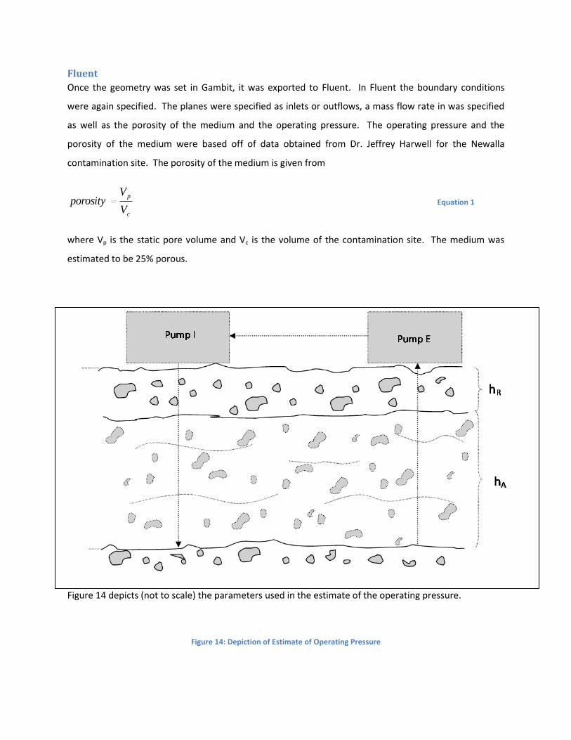
Fluent
Once the geometry was set in Gambit, it was exported to Fluent. In Fluent the boundary conditions
were again specified. The planes were specified as inlets or outflows, a mass flow rate in was specified
as well as the porosity of the medium and the operating pressure. The operating pressure and the
porosity of the medium were based off of data obtained from Dr. Jeffrey Harwell for the Newalla
contamination site. The porosity of the medium is given from
c
p
V
Vporosity Equation 1
where Vp is the static pore volume and Vc is the volume of the contamination site. The medium was
estimated to be 25% porous.
Figure 14 depicts (not to scale) the parameters used in the estimate of the operating pressure.
Figure 14: Depiction of Estimate of Operating Pressure

The operating pressure was estimated by atmMmedia PghP Equation 2 and
RAM hhh Equation 3 where ρmedia is the density of the media, P is the operating pressure,
Patm is atmospheric pressure and g is gravity.
atmMmedia PghP Equation 2
RAM hhh Equation 3
This gave and operating pressure of 205.205 kPa. Also, the size of the aquifer was scaled by equating
each unit in the Gambit mesh to 1 meter. In other words, the 20 × 10 × 10 geometry equated to a 2000
m3 volume aquifer.
These parameters were input into Fluent for simulations. In order to analyze the flow through
the aquifer, imaginary planes were drawn into the Fluent geometry.
Figure 15: Imaginary Planes in Fluent and Nomenclature

After simulations were run, Fluent would output the mass flow rate through each plane. For this
analysis, imaginary planes were drawn down the length (x-direction) of the aquifer volume. The
imaginary planes through the aquifer are shown in Figure 16. The nomenclature for these imaginary
planes are as follows:
The first letter in the name indicates the location of the plane in the specific slice (Figure 15)
The number in the name of the plane indicates the slice number in which the plane is located
(Figure 16)
Figure 16: Planes Through the Length of the Aquifer
Initial Fluid Flow Simulations
Simulations were run for each of the well configurations. Flow rate was varied for each well
configuration. The flow rates tested were 100, 50, 10, 5, 1, 0.5 and 0.1 kg/s. A constant pumping rate
over the entire remediation time was assumed. Also, to keep from creating accumulation or movement
of the plume, it is required that the total mass flow in be equal to the total mass flow out of the aquifer.
In order to get an understanding of the behavior of the fluid flow in the aquifer with the various well
configurations, the path lines were examined. An example of the behavior for the fluid flow in the
aquifer with configuration 1 is shown in Figure 17. The color scale is given for the velocities along the
Slice
Number
9 6 3 0 -3 -6 -9

path lines. It is clear that the highest velocities in the aquifer are along the centerline. This is expected
because the water is flowing directly from the inlet to the outlet. It can also be seen that because the
amount of water being pumped into the aquifer, 1 kg/s, is so small compared to the volume of the
aquifer, the velocity at any point in the aquifer is very small. The highest velocity in the aquifer with this
flow rate and well configuration is about 2.67 × 10⁻⁴ m/s. Figure 18 through Figure 23 show the path
lines for the fluid flow for several other configurations.
Figure 17: Path Lines for Configuration 1
Configuration 1
Flow Rate = 1 kg/s
Configuration 2

Figure 18: Path Lines for Configuration 2
Figure 19: Path Lines for Configuration 3
Flow Rate = 50 kg/s
Configuration 3
Flow Rate = 50 kg/s
Configuration 4

Figure 20: Path Lines for Configuration 4
Configuration 5
inlets
outlet
Flow Rate = 50 kg/s

Figure 21: Path Lines for Configuration 5
Figure 22: Path Lines for Configuration 6
Flow Rate = 5 kg/s
Flow Rate = 50 kg/s
Configuration 6

Figure 23: Path Lines for Configuration 7
Another way to visualize the behavior of the fluid flow within the aquifer is to display the velocity
contours at a specific slice in the aquifer. Displaying imaginary planes a-q at slice -9 (closest to the inlet)
and slice 9 (closes to the outlet) for configuration 7 is shown in Figure 24.
e
Figure 24: Velocity Contours for Configuration 7 Slices -9 and 9
Configuration 7
Flow Rate = 5 kg/s
Flow Rate = 5 kg/s
Configuration 7

It can be seen that the velocity is very high through each of the inlets. By the time the water reaches the
outlets, some of the water drags the water in the middle of the aquifer and leads to some movement in
the middle of the aquifer. It also leads to the spread of the velocity profile at each of the outlets.
Figure 25: Velocity Contours for Configuration 5 Slices -9 and 9
Fluent was used to give the mass flow rate of water through each of the imaginary planes in the aquifer
for each of the well configurations and flow rates.
Concentration Profiles
The concentration profiles for the various well configurations and flow rates were calculated in Excel.
The flow of water through the planes was treated as a “front” of water. It was seen that the water
entering through the inlet is not causing large amounts of mixing in the aquifer but was more pushing
the contaminated water toward the outlets. This phenomenon is depicted in Figure 26.
Configuration 5
Flow Rate = 5 kg/s

Figure 26: Front of Water Traveling Through the Aquifer
This depiction is not entirely accurate, however, since the velocity through the different planes will not
be the same (i.e. the velocity through the center plane, M, will not be the same as one of the outer
planes such as plane A for this configuration). A more accurate depiction of how the fronts of water
would move through the aquifer in configuration 1 is shown in Figure 27.
Figure 27: Fronts of Water Through the Aquifer for Configuration 1
An example of how this phenomenon might appear for configuration 5 is shown in Figure 28.
Inlet
Outlet
Plane of
Water

Figure 28: Fronts of Water Through the Aquifer for Configuration 5
The middle section of planes would be expected to move fastest through the aquifer based on the
geometry and the fluid flow characteristics generated by Fluent for this configuration. Using these
behaviors, the concentration profiles were analyzed.
Construction of Concentration Profiles from Fluent Data
Fluent provides a mass flux through a given plane in the simulation volume. Since the flow is at steady
state it is assumed that the flux will not change with time. The volume is broken up into the planes
described previously in the Initial Fluid Flow Approach, Gambit section. At time t = 0, the aquifer was
assumed to be well-mixed and was assumed to have a uniform initial concentration. The flux through
each of the planes is averaged along the x-axis to get a constant flux through each of the planes. Next
the volume between each of the planes is calculated using the size of and spacing between each of the
planes. From this information and the following equation the concentration profile with time and
position can be formulated for any given initial concentration.

V
tCFtCFCVC inouto
f
)()()( Equation 4
where cf is final concentration, V is the volume between planes, c0 is initial concentration in the volume
being calculated, cout is the concentration leaving, cin is the concentration entering, F is the flux through
the given plane and ∆t is the change in time. Fluent not only provides the magnitude of the flux through
the plane, but also the direction of that flux depending on whether the flux is specified to be in the
positive or negative direction. This information complicates the execution of the above formula. The
inlet and outlet concentrations are decided by the direction of the flux. If the flux passes in the forward
direction, then the inlet concentration comes from the previous volume (the volume in the negative x
direction), and the outlet concentration comes from the current volume. If, however, the flux is
negative, then the inlet concentration comes from the following volume (the volume in the positive x
direction) and the outlet concentration comes from the current volume. For clarification on these
fluxes, directions, and concentrations, refer to Figure 29 below. If, for example, the flux through Plane A
in Figure 29: Method for Determining Concentration In and Out of the Plane is positive then the flux will
be moving into the volume between Planes A and B. The flux will be added (going in to the volume) and
the concentration which will be entering through Plane A is cprevious. Conversely, if the flux through Plane
A is negative, the flux will be moving in the negative x direction out of the volume and the concentration
used will be c0. If the flux through Plane B is positive, the flux will be leaving the volume between Plane
A and Plane B, and the concentration which will be leaving is c0. A negative flux through Plane B will
result in concentration cnext entering the volume between Planes A and B.
Figure 29: Method for Determining Concentration In and Out of the Plane
cprevious cnext
C0
x
Positive
Flow
Negative
Flow
Plane A
Plane B
Plane A
Plane B

This calculation is performed sequentially with respect to both time and position. The result is a
concentration profile that is a function of both position in the aquifer and time. The overall final
concentration is found by taking the average of the concentrations in each of the planes. To achieve
the desired concentration inside the aquifer, solver is used to set the final concentration to the proper
EPA specification by changing delta t. This gives the overall remediation time and concentration profile.
Once these are found, an economic analysis can be performed to find the optimum well configuration
and flow rate.
Results and Discussion
An example application was performed to test the model. Several case studies, including a groundwater
remediation site in Newalla, Oklahoma (courtesy of Dr. Jeffrey Harwell) and an example by Chang et al.,
were referenced to find realistic aquifer properties. The characteristics chosen for the simulations are
displayed in Error! Reference source not found. below.
Aquifer properties
Media Bulk density 2.12 g/cm3
Porosity 0.25
Width 10 m
Length 20 m
Depth 10 m
Contaminant Benzene
Initial Concentration 0.0001 kg/L
Injection Concentration 0.0000 kg/L
Desired Concentration 3.15 x 10⁶ kg/L Table 8: Aquifer Properties
Each of the well configurations was run in Fluent at seven different flow rates: 0.1, 0.5, 1, 5, 10, 50, and
100 kg/s. The total flow rate was the same for each of the configurations, only the amount pumped at
each well was changed with the configuration. Fluent provided the mass flux through all of the
imaginary planes and these were then converted into volumetric flow rates using the density of water.
Contaminant concentrations are too low to have an effect on the density, thus it is valid to assume a
density of 1 kg/L. The volumetric flow rate was then multiplied by the concentration to find the mass
flux of contaminant through the plane. The initial mass of contaminant between the planes is known.
Thus, these values can be plugged into V
tCFtCFCVC inouto
f
)()()(

Equation 4 to perform a
mass balance between the planes and produce a concentration profile of the aquifer.
The data for several of the planes in each configuration is analyzed at a flow rate of 5 kg/s. This flow
rate was chosen because it is a flow rate which is the median value for the flow rates to be investigated.
The results for planes A, D, and M in Configuration 1 at a flow rate of 5 kg/s are displayed in Figure 30
through Figure 32 below. Planes A, D, and M were chosen to give a varied view of the flow behavior
throughout the aquifer.
Figure 30: Concentration vs Time for Plane A, Configuration 1, 5 kg/s
0
0.00002
0.00004
0.00006
0.00008
0.0001
0.00012
0 5 10 15 20 25 30 35
Co
nce
ntr
atio
n (
kg/L
)
Time (days)
Concentration vs Time for Plane A
A-9
A-6
A-3
A0
A3
A6
A9
Flow Rate = 5 kg/sConfiguration 1

Figure 31: Concentration vs Time for Plane D, Configuration 1, 5 kg/s
Figure 32: Concentration vs Time for Plane M, Configuration 1, 5 kg/s
In configuration 1 there is only 1 inlet and 1 outlet and both are positioned in the center of their
respective faces on the simulation volume. This causes the fastest velocities to be in the center of the
0
0.00002
0.00004
0.00006
0.00008
0.0001
0.00012
0 5 10 15 20 25 30 35
Co
nce
ntr
atio
n (
kg/L
)
Time (days)
Concentration vs Time for Plane D
D-9
D-6
D-3
D0
D3
D6
D9
Flow Rate = 5 kg/sConfiguration 1
0
0.00002
0.00004
0.00006
0.00008
0.0001
0.00012
0 5 10 15 20 25 30 35
Co
nce
ntr
atio
n (
kg/L
)
Time (days)
Concentration vs Time for Plane M
M-9
M-6
M-3
M0
M3
M6
M9
Flow Rate = 5 kg/sConfiguration 1

aquifer. This is why Plane M (the very center plane) is immediately clean (See Figure 32). Planes A and
D however, are along the edges of the volume where the velocity is much slower leading to a more
subtle decrease in concentration as opposed to the step function seen in Plane M. This slower change
also results in a longer remediation time for the entire aquifer.
The same planes and flow rate that are analyzed above are used in Configuration 2. These results are
exhibited in Figure 33 through Figure 35.
Figure 33: Concentration vs Time for Plane A, Configuration 2, 5 kg/s
0
0.00002
0.00004
0.00006
0.00008
0.0001
0.00012
0 1 2 3 4 5 6 7
Co
nce
ntr
atio
n (
kg/L
)
Time (days)
Concentration vs Time for Plane A
A-9
A-6
A-3
A0
A3
A6
A9
Flow Rate = 5 kg/sConfiguration 2

Figure 34: Concentration vs Time for Plane D, Configuration 2, 5 kg/s
Figure 35: Concentration vs Time for Plane M, Configuration 2, 5 kg/s
0
0.00002
0.00004
0.00006
0.00008
0.0001
0.00012
0 1 2 3 4 5 6 7
Co
nce
ntr
atio
n (
kg/L
)
Time (days)
Concentration vs Time for Plane D
D-9
D-6
D-3
D0
D3
D6
D9
Flow Rate = 5 kg/sConfiguration 2
0
0.00002
0.00004
0.00006
0.00008
0.0001
0.00012
0 1 2 3 4 5 6 7
Co
nce
ntr
atio
n (
kg/L
)
Time (days)
Concentration vs Time for Plane M
M-9
M-6
M-3
M0
M3
M6
M9
Flow Rate = 5 kg/sConfiguration 2

Configuration 2 consists of 1 inlet and 2 outlets. This gives a very similar flow profile to the 1 inlet, 1
outlet configuration, except that the fast velocities are more widespread in the z-direction. This is
illustrated by the step function displayed in Plane D aswell as Plane M. The contaminant change in Plane
A is more gradual because the flux through any given x-coordinate is always the same, and in this
configuration there is increased flow in other planes taking flow away from Plane A.
The concentration plots of configuration 3 can be seen in Figure 36 through Figure 38 below.
Figure 36: Concentration vs Time for Plane D, Configuration 3, 5 kg/s
0
0.00002
0.00004
0.00006
0.00008
0.0001
0.00012
0 2 4 6 8 10 12 14
Co
nce
ntr
atio
n (
kg/L
)
Time (days)
Concentration vs Time for Plane A
A-9
A-6
A-3
A0
A3
A6
A9
Flow Rate = 5 kg/sConfiguration 3

Figure 37: Concentration vs Time for Plane D, Configuration 3, 5 kg/s
Figure 38: Concentration vs Time for Plane M, Configuration 3, 5 kg/s
0
0.00002
0.00004
0.00006
0.00008
0.0001
0.00012
0 2 4 6 8 10 12 14
Co
nce
ntr
atio
n (
kg/L
)
Time (days)
Concentration vs Time for Plane D
D-9
D-6
D-3
D0
D3
D6
D9
Flow Rate = 5 kg/sConfiguration 3
0
0.00002
0.00004
0.00006
0.00008
0.0001
0.00012
0 2 4 6 8 10 12 14
Co
nce
ntr
atio
n (
kg/L
)
Time (days)
Concentration vs Time for Plane M
M-9
M-6
M-3
M0
M3
M6
M9
Flow Rate = 5 kg/sConfiguration 3

Configuration 3 is made up of 1 inlet and 3 outlets. The outlets are arranged in a triangle with two near
the bottom and one near the top of the aquifer. The flow is more widespread due to the multiple
outlets and their more expansive positioning. This leads to the step functions observed in Planes D and
M, and the steeper decrease seen in Plane A. The three outlets allow a more even distribution in the
velocities which in turn cleans the entire aquifer more quickly.
In Figure 39 through Figure 44 below Configurations 4 and 5 are presented. Arrangement 4 consists of 2
inlets and 1 outlets, and arrangement 5 consists of 2 inlets and 2 outlets.
Figure 39: Concentration vs Time for Plane A, Configuration 4, 5 kg/s
0
0.00002
0.00004
0.00006
0.00008
0.0001
0.00012
0 5 10 15 20 25 30
Co
nce
ntr
atio
n (
kg/L
)
Time (days)
Concentration vs Time for Plane A
A-9
A-6
A-3
A0
A3
A6
A9
Flow Rate = 5 kg/sConfiguration 4

Figure 40: Concentration vs Time for Plane D, Configuration 4, 5 kg/s
Figure 41: Concentration vs Time for Plane M, Configuration 4, 5 kg/s
0
0.00002
0.00004
0.00006
0.00008
0.0001
0.00012
0 5 10 15 20 25 30
Co
nce
ntr
atio
n (
kg/L
)
Time (days)
Concentration vs Time for Plane D
D-9
D-6
D-3
D0
D3
D6
D9
Flow Rate = 5 kg/sConfiguration 4
0
0.00002
0.00004
0.00006
0.00008
0.0001
0.00012
0 5 10 15 20 25 30
Co
nce
ntr
atio
n (
kg/L
)
Time (days)
Concentration vs Time for Plane M
M-9
M-6
M-3
M0
M3
M6
M9
Flow Rate = 5 kg/sConfiguration 4
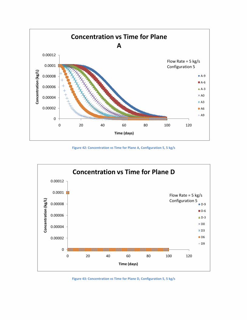
Figure 42: Concentration vs Time for Plane A, Configuration 5, 5 kg/s
Figure 43: Concentration vs Time for Plane D, Configuration 5, 5 kg/s
0
0.00002
0.00004
0.00006
0.00008
0.0001
0.00012
0 20 40 60 80 100 120
Co
nce
ntr
atio
n (
kg/L
)
Time (days)
Concentration vs Time for Plane A
A-9
A-6
A-3
A0
A3
A6
A9
Flow Rate = 5 kg/sConfiguration 5
0
0.00002
0.00004
0.00006
0.00008
0.0001
0.00012
0 20 40 60 80 100 120
Co
nce
ntr
atio
n (
kg/L
)
Time (days)
Concentration vs Time for Plane D
D-9
D-6
D-3
D0
D3
D6
D9
Flow Rate = 5 kg/sConfiguration 5

Figure 44: Concentration vs Time for Plane M, Configuration 5, 5 kg/s
These setups give results almost identical to Configuration number 2. Again The flow spreads out in the
z-direction, but not the y-direction, resulting in a larger flux in Plane D, but a lower flux, and more
gradual concentration profile in Plane A.
Configuration 6 is comprised of 4 inlets and 1 outlet, the resulting concentration profiles can be seen
below in Figure 45 through Figure 47.
0
0.00002
0.00004
0.00006
0.00008
0.0001
0.00012
0 20 40 60 80 100 120
Co
nce
ntr
atio
n (
kg/L
)
Time (days)
Concentration vs Time for Plane M
M-9
M-6
M-3
M0
M3
M6
M9
Flow Rate = 5 kg/sConfiguration 5

Figure 45: Concentration vs Time for Plane A, Configuration 6, 5 kg/s
Figure 46: Concentration vs Time for Plane D, Configuration 6, 5 kg/s
0
0.00002
0.00004
0.00006
0.00008
0.0001
0.00012
0 0.5 1 1.5 2
Co
nce
ntr
atio
n (
kg/L
)
Time (days)
Concentration vs Time for Plane A
A-9
A-6
A-3
A0
A3
A6
A9
Flow Rate = 5 kg/sConfiguration 6
0
0.00002
0.00004
0.00006
0.00008
0.0001
0.00012
0 10 20 30 40 50 60 70 80 90
Co
nce
ntr
atio
n (
kg/L
)
Time (days)
Concentration vs Time for Plane D
D-9
D-6
D-3
D0
D3
D6
D9
Flow Rate = 5 kg/sConfiguration 6

Figure 47: Concentration vs Time for Plane M, Configuration 6, 5 kg/s
The 4 inlets are placed near the corners, and the 1 outlet is in the center of the simulation volume. This
causes the flow to travel mainly through the corners and the center with some dispersion to the sides
producing an instant concentration decrease in Planes A and M, and a more gradual decrease in Plane D.
The outcome of the final arrangement simulated, Configuration 7, can be seen in Figure 48 through
Figure 50 below.
0
0.00002
0.00004
0.00006
0.00008
0.0001
0.00012
0 10 20 30 40 50 60 70 80 90
Co
nce
ntr
atio
n (
kg/L
)
Time (days)
Concentration vs Time for Plane M
M-9
M-6
M-3
M0
M3
M6
M9
Flow Rate = 5 kg/sConfiguration 6
0
0.00002
0.00004
0.00006
0.00008
0.0001
0.00012
0 2 4 6 8 10 12
Co
nce
ntr
atio
n (
kg/L
)
Time (days)
Concentration vs Time for Plane A
A-9
A-6
A-3
A0
A3
A6
A9
Flow Rate = 5 kg/sConfiguration 7

Figure 48: Concentration vs Time for Plane A, Configuration 7, 5 kg/s
Figure 49: Concentration vs Time for Plane D, Configuration 7, 5 kg/s
Figure 50: Concentration vs Time for Plane M, Configuration 7, 5 kg/s
This design includes 4 inlets and 4 outlets all placed near the corners of the aquifer. In this simulation
the flow remained primarily in the corners consequently giving an instant concentration drop in Plane A,
and a gentle decrease through the center planes.
0
0.00002
0.00004
0.00006
0.00008
0.0001
0.00012
0 2 4 6 8 10 12
Co
nce
ntr
atio
n (
kg/L
)
Time (days)
Concentration vs Time for Plane D
D-9
D-6
D-3
D0
D3
D6
D9
Flow Rate = 5 kg/sConfiguration 7
0
0.00002
0.00004
0.00006
0.00008
0.0001
0.00012
0 2 4 6 8 10 12
Co
nce
ntr
atio
n (
kg/L
)
Time (days)
Concentration vs Time for Plane M
M-9
M-6
M-3
M0
M3
M6
M9
Flow Rate = 5 kg/sConfiguration 7

Below in Figure 51 is a graph of the overall aquifer concentration vs time with configuration as a
parameter.
Figure 51: Average Concentration vs Time with 5 kg/s and Configuration as a Parameter
The well configuration has a highly pronounced effect on the remediation time. This is due to the
distribution of the clean injected water. The designs with fewer number of extraction wells than
number of inlet wells were observed to perform the slowest. This is because when the streams are
narrowed to only one outlet they are unable to flow through all areas and, as a result, the arrangement
cannot effectively clean the entire aquifer. Along the same lines, arrangements with the same number
of inlets and outlets being positioned in the same z and y coordinates are not highly effective. This is
because flow is forced directly from the inlet to outlet and does not radiate in the z or y directions. This
leaves many essentially stagnant regions in the aquifer. Conversely, the formations that posess one
inlet and several outlets are able to rid the aquifer of contaminants more efficiently because the flow
can disperse more uniformly in all three dimensions.
Displayed below in Figure 52 is a comparison between remediation time and flow rates with
configuration as a parameter.
0
0.00002
0.00004
0.00006
0.00008
0.0001
0.00012
0 20 40 60 80 100 120
Co
nce
ntr
atio
n (
kg/L
)
Time (days)
Average Concentration vs Time
Configuration 1
Configuration 2
Configuration 3
Configuration 4
Configuration 5
Configuration 6
Configuration 7
Flow Rate = 5 kg/s
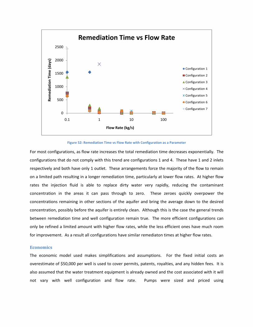
Figure 52: Remediation Time vs Flow Rate with Configuration as a Parameter
For most configurations, as flow rate increases the total remediation time decreases exponentially. The
configurations that do not comply with this trend are configurations 1 and 4. These have 1 and 2 inlets
respectively and both have only 1 outlet. These arrangements force the majority of the flow to remain
on a limited path resulting in a longer remediation time, particularly at lower flow rates. At higher flow
rates the injection fluid is able to replace dirty water very rapidly, reducing the contaminant
concentration in the areas it can pass through to zero. These zeroes quickly overpower the
concentrations remaining in other sections of the aquifer and bring the average down to the desired
concentration, possibly before the aquifer is entirely clean. Although this is the case the general trends
between remediation time and well configuration remain true. The more efficient configurations can
only be refined a limited amount with higher flow rates, while the less efficient ones have much room
for improvement. As a result all configurations have similar remediaton times at higher flow rates.
Economics
The economic model used makes simplifications and assumptions. For the fixed initial costs an
overestimate of $50,000 per well is used to cover permits, patents, royalties, and any hidden fees. It is
also assumed that the water treatment equipment is already owned and the cost associated with it will
not vary with well configuration and flow rate. Pumps were sized and priced using
0
500
1000
1500
2000
2500
0.1 1 10 100
Re
me
dia
tio
n T
ime
(d
ays)
Flow Rate (kg/s)
Remediation Time vs Flow Rate
Configuration 1
Configuration 2
Configuration 3
Configuration 4
Configuration 5
Configuration 6
Configuration 7

FVVPP
zzg2
2
1
2
21212
Equation 6 , the Bernoulli
equation, and Peters & Timmerhaus. It is also assumed that fixed continuous costs will remain constant
regardless of arrangement and pumping rate. Within the variable continuous costs, water treatment is
considered on a price per liter basis, labor costs were extracted from the U.S. department of Labor, and
utilities were calculated using Peters & Timmerhaus.
These parameters were combined in
yElectricitPumpmentWatertreatDrillingLaborCost Equation 5
yElectricitPumpmentWatertreatDrillingLaborCost Equation 5
Labor costs are comprised of:
Management
Engineers
Scientists
Construction/Maintenance
The national average of wages for these positions in the watertreatment industry were found and then
multiplied by the number of employees in each position and then by the number of hours necessary for
the project. The drilling costs were calculated by multiplying the number of wells by the standard
$50,000 per well. Watertreatment costs were strictly based on a $0.053 per liter treatment price. The
Pump was sized using
FVVPP
zzg2
2
1
2
21212
Equation 6.
FVVPP
zzg2
2
1
2
21212
Equation 6
g = gravity z2 = final height z1 = initial height P2 = final pressure P2 = initial pressure ρ = density V2 = final velocity V1 = initial velocity ∑F = frictional losses

The frictional losses were calculated by combining
vDRe
Equation 7 through
g
v
D
Lfh fL
2
2
Equation 9.
vDRe Equation 7
Re = Reynold’s Number D = diameter ρ = density v = velocity υ = viscosity
Re
16ff Equation 8
ff = fanning friction factor
g
v
D
Lfh fL
2
2 Equation 9
hL = head loss L = Length D = Diameter v = velocity g = gravity
Once the head of the pump is calculated using the Bernoulli equation, figure 12-19 in Peters and
Timmerhaus is used to price the pump and find the power required by the pump. This pump price is
then multiplied by the number of pumps necessary. Due to the pressure gradient between the outlet of
the extraction well (at the surface) and the inlet of the extraction well (in the aquifer), natural flow was
assumed and pumping for extraction wells was neglected. Electricity cost is then calculated by
multiplying the power required by the pump by the number of pumps, then by the number of hours,
and finally by $0.0969 per kWh.
This economic analysis was performed on each of the simulations run, and the results were compared to
find the most economic configuration and flow rate. The least expensive flow rates for each
arrangement were compared to determine the optimal remediation design. These results are displayed
in Table 9.
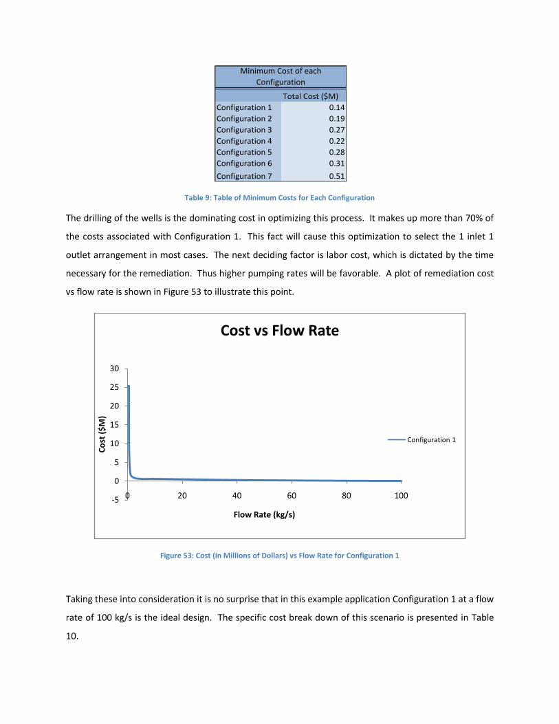
Table 9: Table of Minimum Costs for Each Configuration
The drilling of the wells is the dominating cost in optimizing this process. It makes up more than 70% of
the costs associated with Configuration 1. This fact will cause this optimization to select the 1 inlet 1
outlet arrangement in most cases. The next deciding factor is labor cost, which is dictated by the time
necessary for the remediation. Thus higher pumping rates will be favorable. A plot of remediation cost
vs flow rate is shown in Figure 53 to illustrate this point.
Figure 53: Cost (in Millions of Dollars) vs Flow Rate for Configuration 1
Taking these into consideration it is no surprise that in this example application Configuration 1 at a flow
rate of 100 kg/s is the ideal design. The specific cost break down of this scenario is presented in Table
10.
Total Cost ($M)
Configuration 1 0.14
Configuration 2 0.19
Configuration 3 0.27
Configuration 4 0.22
Configuration 5 0.28
Configuration 6 0.31
Configuration 7 0.51
Minimum Cost of each
Configuration
-5
0
5
10
15
20
25
30
0 20 40 60 80 100
Co
st (
$M
)
Flow Rate (kg/s)
Cost vs Flow Rate
Configuration 1

Table 10: Cost Breakdown for Configuration 1 with 100 kg/s
Secondary Fluid Flow Approach
The aim of the secondary fluid flow simulations was to build upon the accuracy and complexity of the
previous simulations and modeling. The path in which this was accomplished was by analyzing the
cleaning of an aquifer, which had a non-uniform initial concentration profile, and by creating a more
realistic aquifer geometry. Total pumping rate through the aquifer was chosen to have a value closer to
flow rates that would be used in industrial practices for cleaning of this type of aquifer. This adjustment
was made because the flow rates analyzed in the previous model were somewhat unrealistic for use in
actual application. New approaches were taken to minimize remediation time and contamination in the
plumes because an economic optimum can be met by minimizing remediation time while achieving
highest possible purification. In this secondary approach, well location was also reformed to parallel
industrial practice. Specifically, wells were positioned along the top of the aquifer in order to allow for
placement of adjacent inlets and outlets. This is a practice that is standard in many concrete
applications, as is seen in the Newalla site. Lastly, because many contamination distributions are
generally non-uniform, three separate shapes of plumes with unique initial concentration profiles were
created for remediation analysis. Pumping strategies for the cleaning of the plumes were designed for
each scheme. The first step of this method was to create a new geometry in Gambit.
Gambit
The geometry of the aquifer and pumping arrangement were redesigned in order to create simulations
that are more realistic to characteristics seen in industry. One of the first important changes was to
create a geometry where the wells have inlets and outlets in the middle of the aquifer. This geometry
was created to simulate pipes drilled into the center of the well from the top of the aquifer. Another

change from the previous model is that the new geometry uses a 40 × 20 × 10 volume. This yields a
volume of 8000 m3. The flow rate used in the aquifer was then scaled according to the flow rate relative
to the total volume, using the Newalla site as the reference values. In other words, since the total
volume of the Newalla plume is 2150 m3 and the Newalla site uses a total flow rate through all the inlets
of approximately 0.4 kg/s, scaling this up to clean an 8000 m3 aquifer, the total flow rate through the
aquifer should be approximately 1.5 kg/s. For each configuration used, this value is divided by the total
number of inlets to find the flow rate through each inlet. It is key to clarify that for any configuration,
the pumping rate through a given well does not change with time. Also, the total mass being injected,
which is the sum of the flow rate through each injection, is always constant. It is only the injection and
extraction points that change at a point in time. The new generic geometry drawn for these simulations
is shown in Figure 54.
Figure 54: Refined Generic Geometry
The nomenclature for the naming of these wells is shown in Figure 55.

Figure 55: Nomenclature for Naming of Faces for Wells
Again, the faces may be designated as “on” or “off” depending on whether their boundary condition is
specified to be a mass-flow inlet, outflow, or wall.
Initial Plume Profiles
The three initial plume profiles that were created are as follows
Plume 1: A “rectangular” shaped plume
Plume 2: A “figure 8” shaped plume
Plume 3: A “moon shaped” plume
The general shapes of the plumes, colored by contamination concentration, are shown in Figure 56.

It can be seen in Figure 56 that the highest concentrations are located toward the inner part of the
aquifer in each plume profile, with the highest concentration being represented by the darkest gray and
the smallest concentration being shown in the lightest gray.
Pumping Strategies
To remediate the contamination problems in the three plumes, a unique pumping strategy was designed
for each. The initial plume profile and its corresponding pumping strategy is shown in
Figure 57 through Figure 59 below. In the pumping strategies, the blue faces will be designated mass
flow inlets and the red faces will be designated as outflows. The white faces will be “off,” or will be
treated as walls.
a1 b1 c1 d1
a2 b2 c2 d2
a3 b3 c3 d3
a4 b4 c4 d4
a5 b5 c5 d5
a6 b6 c6 d6
a7 b7 c7 d7
a1 b1 c1 d1
a2 b2 c2 d2
a3 b3 c3 d3
a4 b4 c4 d4
a5 b5 c5 d5
a6 b6 c6 d6
a7 b7 c7 d7
a1 b1 c1 d1
a2 b2 c2 d2
a3 b3 c3 d3
a4 b4 c4 d4
a5 b5 c5 d5
a6 b6 c6 d6
a7 b7 c7 d7
kg/L
kg/L
kg/L
kg/L
0.000200
0.000150
0.000025
0.000100
Figure 56: Non-Uniform Initial Concentration Profiles
Plume 1 Step 1 Step 2 Step 3
Plume 1 Plume 2 Plume 3

Figure 57: Pumping Strategy for Plume 1
Figure 58: Pumping Strategy for Plume 2
Figure 59: Pumping Strategy for Plume 3
The idea behind these pumping strategies is to attempt to push all of the contaminants, by pumping in
clean water, toward the outflow locations where the contaminant-rich water will be removed from the
aquifer.
a1 b1 c1 d1
a2 b2 c2 d2
a3 b3 c3 d3
a4 b4 c4 d4
a5 b5 c5 d5
a6 b6 c6 d6
a7 b7 c7 d7
a1 b1 c1 d1
a2 b2 c2 d2
a3 b3 c3 d3
a4 b4 c4 d4
a5 b5 c5 d5
a6 b6 c6 d6
a7 b7 c7 d7
a1 b1 c1 d1
a2 b2 c2 d2
a3 b3 c3 d3
a4 b4 c4 d4
a5 b5 c5 d5
a6 b6 c6 d6
a7 b7 c7 d7
a1 b1 c1 d1
a2 b2 c2 d2
a3 b3 c3 d3
a4 b4 c4 d4
a5 b5 c5 d5
a6 b6 c6 d6
a7 b7 c7 d7
a1 b1 c1 d1
a2 b2 c2 d2
a3 b3 c3 d3
a4 b4 c4 d4
a5 b5 c5 d5
a6 b6 c6 d6
a7 b7 c7 d7
a1 b1 c1 d1
a2 b2 c2 d2
a3 b3 c3 d3
a4 b4 c4 d4
a5 b5 c5 d5
a6 b6 c6 d6
a7 b7 c7 d7
Plume 2 Step 1 Step 2 Step 3
Plume 3 Step 1 Step 2 Step 3

Secondary Fluid Flow Simulations
Fluent The geometry drawn in Gambit was imported into Fluent. Vertical planes were drawn in Fluent. Secondary simulations
Secondary simulations utilized more vertical planes than were in the initial fluid flow simulations in order to increase order to increase accuracy in the measurement of flux through the aquifer. The nomenclature for naming the vertical planes
naming the vertical planes is shown in f
Figure 60 below.
Figure 60: Vertical Planes in Fluent
The total number of vertical planes drawn for secondary simulations was 500. These planes were, again,
drawn and named individually. Since the well configuration in these secondary trials creates more flow
in the y direction, horizontal planes were also drawn below the bottom of the pipes in the aquifer. The
nomenclature for naming the horizontal planes and some depictions of their locations in the aquifer is
given in
pa1 pb1 pc1 pd1 pe1
pa2 pb2 pc2 pd2 pe2
pa3 pb3 pc3 pd3 pe3
pa4 pb4 pc4 pd4 pe4
pa5 pb5 pc5 pd5 pe5
pa6 pb6 pc6 pd6 pe6
pa7 pb7 pc7 pd7 pe7
pa8 pb8 pc8 pd8 pe8
pa9 pb9 pc9 pd9 pe9
pa10 pb10 pc10 pd10 pe10

Figure 61.
Figure 61: Layout and Nomenclature for Naming Horizontal Planes
Once the planes were drawn and named, several initial trials were run with different well configurations
in order to examine the behavior of the flow with the new pipe and aquifer arrangement. Figures
showing the arrangement of the wells and the resulting profiles are shown below. These profiles are, as
in the primary fluid flow approach, path lines colored by velocity.
A B C D E
-14
-10
-6
-2
2
6
10
14
18

.
a1 b1 c1 d1
a2 b2 c2 d2
a3 b3 c3 d3
a4 b4 c4 d4
a5 b5 c5 d5
a6 b6 c6 d6
a7 b7 c7 d7
a1 b1 c1 d1
a2 b2 c2 d2
a3 b3 c3 d3
a4 b4 c4 d4
a5 b5 c5 d5
a6 b6 c6 d6
a7 b7 c7 d7

a1 b1 c1 d1
a2 b2 c2 d2
a3 b3 c3 d3
a4 b4 c4 d4
a5 b5 c5 d5
a6 b6 c6 d6
a7 b7 c7 d7
a1 b1 c1 d1
a2 b2 c2 d2
a3 b3 c3 d3
a4 b4 c4 d4
a5 b5 c5 d5
a6 b6 c6 d6
a7 b7 c7 d7

Figure 62: Examples of Several Well Configurations Simulated
The testing of these well configurations showed expected flow patterns. This gave validity to the new
geometry and allowed for the pursuit of the new plume treatment and pumping strategy method.
Simulations were next run for the three steps in the pumping strategy for the three different initial
plume profiles. The results for plume profile 1 are shown below in Figure 63.
a1 b1 c1 d1
a2 b2 c2 d2
a3 b3 c3 d3
a4 b4 c4 d4
a5 b5 c5 d5
a6 b6 c6 d6
a7 b7 c7 d7

Figure 63: Plume 1 Steps 1 Through 3
a1 b1 c1 d1
a2 b2 c2 d2
a3 b3 c3 d3
a4 b4 c4 d4
a5 b5 c5 d5
a6 b6 c6 d6
a7 b7 c7 d7
a1 b1 c1 d1
a2 b2 c2 d2
a3 b3 c3 d3
a4 b4 c4 d4
a5 b5 c5 d5
a6 b6 c6 d6
a7 b7 c7 d7
a1 b1 c1 d1
a2 b2 c2 d2
a3 b3 c3 d3
a4 b4 c4 d4
a5 b5 c5 d5
a6 b6 c6 d6
a7 b7 c7 d7

The flow results and configurations depictions for plume 2 are shown in Figure 64.
Figure 64: Plume 2 Steps 1 Through 3
a1 b1 c1 d1
a2 b2 c2 d2
a3 b3 c3 d3
a4 b4 c4 d4
a5 b5 c5 d5
a6 b6 c6 d6
a7 b7 c7 d7
a1 b1 c1 d1
a2 b2 c2 d2
a3 b3 c3 d3
a4 b4 c4 d4
a5 b5 c5 d5
a6 b6 c6 d6
a7 b7 c7 d7
a1 b1 c1 d1
a2 b2 c2 d2
a3 b3 c3 d3
a4 b4 c4 d4
a5 b5 c5 d5
a6 b6 c6 d6
a7 b7 c7 d7

The profiles for steps 1 though 3 of the pumping strategy for plume 3 are shown below.
Figure 65: Plume 3 Steps 1 Thorough 3
a1 b1 c1 d1
a2 b2 c2 d2
a3 b3 c3 d3
a4 b4 c4 d4
a5 b5 c5 d5
a6 b6 c6 d6
a7 b7 c7 d7
a1 b1 c1 d1
a2 b2 c2 d2
a3 b3 c3 d3
a4 b4 c4 d4
a5 b5 c5 d5
a6 b6 c6 d6
a7 b7 c7 d7
a1 b1 c1 d1
a2 b2 c2 d2
a3 b3 c3 d3
a4 b4 c4 d4
a5 b5 c5 d5
a6 b6 c6 d6
a7 b7 c7 d7

In order to more easily visualize where the wells are located in the aquifer, filled contours may be
displayed and colored by velocity. Two examples of these contours are shown in Figure 66 and Figure
67. Figure 66 is step 2 in the cleaning of plume 3 and Figure 67 is step 3 in the cleaning of plume 3.
Figure 66: Velocity Contour for Step 2 of Plume 3
Figure 67: Velocity Contour for Step 3 of Plume 3

Construction of Concentration Profiles from Fluent Data
As discussed earlier, 3 levels of horizontal planes were drawn. These three levels are all below the
mouths of the wells. Because of this, the top half of the aquifer is treated as 9 large boxes. The fluxes
through the sides of the 5 small planes located above the bottom of the pipes (positive y direction) are
added together to create one large flux for the given plane. Visualization of this method is provided in
Figure 68. For these boxes in the top of the aquifer, the mass balance includes the fluxes through the
vertical planes and flux from a bottom horizontal plane. In the bottom half of the aquifer, there are 5
vertical planes that lie in the yz plane for each lettered segment. For the space between the drawn
horizontal planes, an average is taken of the flux through the horizontal planes above and below that
coordinate. The measured fluxes and the average fluxes are then used to calculate the flux into and out
of the boxes in the y direction. This information is then used to calculate concentration profiles as
shown in Figure 69: Schematic for Determining Fluxes for Mass Balance below.
Figure 68: Combining Planes to Make Large Planes in Top of Aquifer
Figure 69: Schematic for Determining Fluxes for Mass Balance
cprevious cnext
cabove
cbelow
cbox
y
z x
pa1 pb1 pc1 pd1 pe1
pa2 pb2 pc2 pd2 pe2
pa3 pb3 pc3 pd3 pe3
pa4 pb4 pc4 pd4 pe4
pa5 pb5 pc5 pd5 pe5
pa6 pb6 pc6 pd6 pe6
pa7 pb7 pc7 pd7 pe7
pa8 pb8 pc8 pd8 pe8
pa9 pb9 pc9 pd9 pe9
pa10 pb10 pc10 pd10 pe10
pa1 pb1 pc1 pd1 pe1
pa2 pb2 pc2 pd2 pe2
pa3 pb3 pc3 pd3 pe3
pa4 pb4 pc4 pd4 pe4
pa5 pb5 pc5 pd5 pe5
pa6 pb6 pc6 pd6 pe6
pa7 pb7 pc7 pd7 pe7
pa8 pb8 pc8 pd8 pe8
pa9 pb9 pc9 pd9 pe9
pa10 pb10 pc10 pd10 pe10
pa1
-5
pb
1-5
pc1
-5
pd
1-5
pe1
-5

The same strategy for calculating the concentration profiles with time using the magnitude and direction
of mass flux through the planes is applied to the refined model with the addition of the flux through the
horizontal planes. Different pumping strategies are examined over a period of approximately 60 days,
and the ending concentrations are compared to determine the configuration which is most efficient in
cleaning.
Results and Discussion
Flow data for the three well configurations were obtained for plume 1. These flow profiles were used to
determine the change in concentration with time for the three configurations individually and with
changing configuration with time. In the dynamic model, configuration was changed when the decrease
in concentration for the previous well arrangement began to plateau. The results of these runs are
displayed in Figure 70 below.
Figure 70: Concentration vs Time for Plume 1
1.5E-05
2.5E-05
3.5E-05
4.5E-05
5.5E-05
6.5E-05
7.5E-05
8.5E-05
9.5E-05
0.000105
0 10 20 30 40 50 60
Co
nta
min
ant
Co
nce
ntr
atio
n (
kg/L
)
Time (days)
Concentration vs TimePlume 1
Configuration 2
Configuration 3
Change
Configuration 1

Figure 71: Plume 1 Profile Colored by Contamination Concentration with Dynamic Optimization
Configuration 1 is the least efficient; it is able to lower the contaminant concentration to 7x10⁻⁵ kg/L and
then it levels off after 7 days. Configuration 2 is the most effective; it reaches lower concentrations
faster and is still decreasing when the 53 day mark is reached. Configuration 3 behaves very similarly to
configuration 2 but is not quite as successful. When the three configurations are combined the aquifer
is cleaned roughly to the same degree as when only configuration 3 is used. However it is initially slower
than configurations 2 and 3. This is because it begins with configuration 1 which is shown to be an
unproductive arrangement. This slower beginning puts this strategy behind initially; in this particular
case, configurations 2 and 3 could be explored for their efficacy in minimizing contaminant
concentration.
The results from the dynamic strategy are used to make concentration profile contours as shown above in
in
Figure 71. After 4 days there is not much noticeable change in the concentration profile, but by day 20
there is a significant difference from the original plume. By day 50 the aquifer is almost completely
clean.
Three new well configurations and the dynamic pumping strategy were applied to the second plume.
The results of these simulations can be seen in Figure 72 below.
4 days 20 days 50 days
10-13-10-8kg/L
10-7-10-6kg/L
10-5
-10-4
kg/L
10-4
-10-3
kg/L

Figure 72: Concentration vs Time for Plume 2
Figure 73: Plume 2 Profiles Colored by Contamination Concentration for Dynamic Optimization
In this plume all four pumping strategies behave very similarly until day 25. At this point configuration 1
reaches its limit and levels out. Configuration 3 also begins to level out and separate from
configurations 2 and the dynamic arrangement.
Contours of concentration profiles are produced from the dynamic pumping simulation. These are
exhibited in Figure 73 above. Just as in the first configuration there is little improvement in 4 days, but
1.5E-05
2.5E-05
3.5E-05
4.5E-05
5.5E-05
6.5E-05
7.5E-05
8.5E-05
9.5E-05
0.000105
0 10 20 30 40 50 60
Co
nta
min
ant
Co
nce
ntr
atio
n (
kg/L
)
Time (days)
Concentration vs TimePlume 2
Configuration 2
Configuration 3
Change
Configuration 1
4 days 20 days 50 days
10-13-10-8kg/L
10-7-10-6kg/L
10-5
-10-4
kg/L
10-4
-10-3
kg/L

when the pumps have been running for 20 days much progress has been made, and by the time 50 days
is reached most of the contaminants have been removed from the aquifer.
The behavior of the third and final plume is presented in Figure 74 below.
Figure 74: Concentration vs Time for Plume 3
Figure 75:Plume 3 Profiles Colored by Contamination Concentration for Dynamic Optimization
1.5E-05
2.5E-05
3.5E-05
4.5E-05
5.5E-05
6.5E-05
7.5E-05
8.5E-05
9.5E-05
0.000105
0 10 20 30 40 50 60Co
nta
min
ant
Co
nce
ntr
atio
n (
kg/L
)
Time (days)
Concentration vs TimePlume 3 Changing Configuration
Configuration 1
Configuration 2
Configuration 3
Change
4 days 20 days 50 days
10-13-10-8kg/L
10-7-10-6kg/L
10-5
-10-4
kg/L
10-4
-10-3
kg/L

In this contamination plume configuration one becomes ineffective at 7 days and levels off.
Configurations 2 and 3 are almost identical. However, the dynamic design behaves very differently from
the first two scenarios. It behaves like a step function at each of the configuration changes. At 40 days
the dynamic system drops below all other configurations becoming the most efficient.
The contamination contours for plume 3 can be found in Figure 75 above. These contours follow the
same pattern as the previous two for t = 4, 20, and 50 days. At the 4 day and 20 day periods it is still
obvious which original contamination profile each contour began with, however, after 50 days, the
overall contamination profile for the three different plumes do not show vast differences between the
cases. In general, all three arrangements show both generally uniform and low contamination profiles.
Further Studies and Future Work
Because of some key assumptions in the formulation of this model, several suggestions can be made for
future studies and continued research. Some areas for improvement upon this model are as follows:
Vary pumping rates for injection and extraction wells with time
Analyze the possibility of injection concentrations greater than zero
Create imaginary planes that lie in the xy plane
Analyze more well configurations
Analyze new plume profiles
Incorporate more geological properties
Account for natural degradation
Incorporate natural flow
Examine more economics
Produce more accurate results for profile near injection and extraction

Conclusions
The initial fluid flow model for the analysis of a pump-treat-inject method remediation of a
contaminated aquifer plume provides a good idea of the time-based concentration profiles in the
aquifer. A wider spread of extraction wells was found to result in a more efficient purification process.
Well configuration was found have a high effect on the flow patterns in the plume. Two adjacent
injection wells, for example, cause high flow directly from the well inlet and cause some drag in the
remaining aquifer volume. Remediation time is inversely related to flow rate. Initial fixed costs,
primarily costs of drilling, dominate the overall cost of remediation. Cleaning time is the next largest
factor in overall cost. The overall time leads to the well number and configuration as well as flow rate
being deciding factors in optimization. The most economical design was found to be using configuration
1 with a flow rate of 100 kg/s. This yields a cost of $140,000.
The secondary fluid flow analysis is more realistic and more accurate. This model may be used to
simulate plumes having different shapes and initial concentration profiles. The secondary fluid flow
analysis technique may be applied as a unique and effective dynamic optimization model. It is shown
that this strategy yields generally good cleaning of contaminants from the plume. The specific efficiency
of the cleaning of a particular aquifer is seen to be highly dependent on the initial shape and profile of
the contamination plume. This dynamic technique can also give more efficient cleaning than a static
optimization model. A plateau is often seen in the cleaning profiles and, often, step changes are also
seen in the contamination concentration. This dynamic optimization has been proven effective
independent of initial plume profile.

Works Cited Agency, T. E. (n.d.). EPA Superfund. Retrieved March 12, 2008, from
http://www.epa.gov/safewater/contaminants/index.html#listmcl
Hanford site. (n.d.). Retrieved February 20, 2008, from Hanford Site Groundwater Remediation Project:
http://www.hanford.gov/cp/gpp/
The Environmental Protection Agency. (n.d.). Retrieved February 19, 2008, from Waterscience:
http://www.epa.gov/waterscience/criteria/drinking/dwstandards.pdf
The Groundwater Foundation. (n.d.). Retrieved February 22, 2008, from National Water-Quality
Assessment Program: http://pubs.usgs.gov/circ/circ1292/pdf/circular1292.pdf
Chang, L.-C., Chu, H.-J., & Hsiao, C. T. (2007). Optimal planning of a dynamic pump-treat-inject
groundwater remediation system. Journal of Hydrology , 295-304.
EPA. (2008). Retrieved 2008, from http://www.epa.gov/safewater/contaminants/index.html#listmcl
Jewell, G. (2008). Hanford site Groundwater remediation project. Retrieved from
http://www.hanford.gov/cp/gpp/
Peters, M. S., Timmerhaus, K. D., & West, R. E. (2003). Plant Design and Economics for Chemical
Engineers. New York: McGraw-Hill.
Tenney, C., & Lastoskie, C. (2007). Pulsed pumping process optimization using a potential flow model.
Journal of Contaminant Hydrology , 111-121.
Welty, J. R., Wicks, C. E., Wilson, R. E., & Rorrer, G. (2001). Fundamentals of Momentum, Heat, and Mass
Transfer. New York: John Wiley & Sons, Inc.