Optimal Auditing for Insurance Fraud*

Georges Dionne1, Florence Giuliano2 and Pierre Picard3

April 10, 2003

* For presentation to the 2003 RTS in Atlanta. Please do not quote without

permission.

1 Risk Management Chair, HEC Montréal, Canada. 2 THEMA, Université de Paris X–Nanterre, France. 3 THEMA, Université de Paris X–Nanterre, CEPREMAP, France.

1

I Introduction In recent years, economic analysis of insurance fraud has developed along two lines. The first one is mostly theoretical and its foundations may be found in the theory of optimal auditing. It aims at analyzing the strategy of insurers under claims fraud or application fraud.1 This approach mainly focuses on questions such as: What should be the frequency of claim auditing and how do opportunistic policyholders react to the auditing strategy? What are the consequences of potential fraud on the design of insurance contracts, especially with regard to the indemnity schedule? What is the deterrence effect of an auditing policy? What is the role of good faith when insurance applicants may misrepresent their risk? The second branch of the literature on insurance fraud is more statistically based: It focuses mainly on the significance of fraud in insurance portfolios; on the practical issue of how insurance fraud can be detected; and on the scope of automated detection mechanisms in lowering the cost of fraudulent claims.2 In this paper, we would like to build bridges between these two complementary approaches to insurance fraud. We will in fact try to reach two objectives: The first one is to establish a connection between the theory of optimal auditing for claims fraud and actual procedures used by insurers to handle claims. The second one tries to characterize the optimal auditing strategy based on data from a large European insurance company in order to lay the foundations of an automated auditing mechanism where detection and deterrence of insurance fraud are simultaneously taken into account. In a few words, the optimal auditing approach to insurance fraud may be summed up as follows. The setting is a costly state verification model in which insureds have private information about their losses and insurers can verify claims by incurring an audit cost. The focus is on the deterrence effect of the auditing strategy and on the consequences of insurance fraud on the design of insurance contracts. Important assumptions are made relative to the ability of insurers to commit to an auditing policy and to the skill of defrauders in manipulating audit costs, i.e. to make the verification of claims more difficult.3 Among the various results reported in this branch of literature, we may mention three. First of all, that optimal auditing should be stochastic. For auditing to deter fraud, the probability of being detected must be positive (but it should be less than one). Secondly, several papers have shown that the problems involved in designing the auditing strategy and specifying insurance contracts are interlinked: For instance, coinsurance may mitigate both the propensity to manipulate audit costs and to falsify claims. Thirdly, commitment to an investigation strategy

1 See Picard (2000) for an overview. 2 See Derrig (2002) and Dionne (2000). See also Dionne and Gagné (2001, 2002), Artis et al. (2002) and Crocker and Tennyson (2002) for different econometric applications. 3 Crocker and Morgan (1997) have developed a costly state falsification approach to insurance fraud which has conceptual similarities with the models of costly state verification with audit cost manipulation. Other references on this issue are Townsend (1979), Crocker and Tennyson (1999) and Picard (1996, 1999).

2

is beneficial: Without this commitment, auditing’s only purpose would be to detect fraudulent claims and no deterrence effect could be achieved. The second branch of the above-mentioned literature on insurance fraud focuses on patterns in claims auditing4: How do insurers actually react to fraud indicators (the so called red flags) and how can automated early detection of fraud be performed. As shown by Derrig (2002) and Tennyson and Salsas-Forn (2002)5 when there is suspicion of fraud, claims are usually handle with a two-stage procedure: after careful examinations, the claim is either paid under routine settlement or subjected to more intensive investigation. This investigation may take different forms: referral to a Special Investigative Unit (SIU); request for recorded or sworn statements from the claimant, the policyholder or a witness to the accident; on site investigation; etc. Furthermore, the reaction to red flags may vary depending on individuals. Developing automated methods capable of using the informational content of red flags as efficiently as possible is currently the subject of really intense research by some insurance companies, particularly in the automobile insurance sector.6 In this paper, we shall link the two branches of the economic literature on insurance fraud by building a costly state verification model to predict an investigation strategy similar to current claims-auditing patterns. We make one important assumption about insurers' access to information: They are supposed to be capable of perceiving claims-related fraud signals. We then calibrate our model by using data on automobile insurance from a large European insurance company and derive the optimal auditing strategy. As a final outcome, our analysis yields an easily automated procedure for detecting insurance fraud. II Model We consider a population of policyholders who differ from one another in the morale cost of filing a fraudulent claim. For the sake of notational simplicity, all individuals own the same initial wealth W and they all face the possibility of a monetary loss L with probability π with 0 < π < 1. We simply describe the event leading to this loss as an “accident.” All individuals are expected to be utility maximizers and to display risk aversion with respect to their wealth. Let u be the state dependent utility of an individual drawn from this population. u depends on final wealth Wf but it also depends on the morale cost incurred in case of insurance fraud:

u = u (Wf, ω) in case of fraud

u = u (Wf, 0) otherwise 4 See the volume 69, no 3, of the Journal of Risk and Insurance, September 2002, for a state-of-the-art presentation of claims fraud detection methods. 5 Derrig (2002); Tennyson and Salmsa-Forn (2002). 6 There is also a literature on the measurement of information problems in economic activity that interprets insurance fraud as an ex-post moral hazard problem. See Chiappori and Salanié (2002) for a recent comprehensive survey.

3

where ω is a non-negative parameter which measures the morale cost of fraud to the policyholder. We assume 0,0 ''

11'1 <> uu and 0'

2 <u and that ω is distributed over +ℜ among the population of policyholders. In other words, individuals who choose to defraud incur more or less high morale costs. Some of them are purely opportunistic (their morale cost is very low) whereas others have a higher sense of honesty (their morale cost is thus higher). Note that morale cost is private information held by the insured: it cannot be observed by the insurer. All the individuals in the insurer portfolio have taken out the same insurance contract. This contract specifies a level of coverage t in case of an accident and a premium P that should be paid to the insurer. Hence, if there is no fraud, we have:

Wf = W – L – P + t in case of an accident and

Wf = W – P if no accident occurs. Each individual in the population is characterized by a vector of observable exogenous variables θ , with θ ∈ Θ ⊂ ℜ m. The morale cost of fraud may be statistically linked to some of these variables. Let ( )θωH be the conditional, cumulated, probability distribution of ω for a type-θ individual, with a density ( )θωh . Our model describes insurance fraud in a very crude way. A defrauder simply files a claim to receive the indemnity payment t although he has not suffered any accident. If a policyholder is detected to have defrauded, he does not receive any insurance payment and in addition he has to pay a fine B to the government.7 Let p be the probability of being detected; this probability is the outcome of the insurer's antifraud policy and it depends on the observable variables θ as we shall see hereafter. When an individual has not suffered any loss, his utility is written as u (W – P, 0) if he does not defraud. If he files a fraudulent claim (i.e. if he claims to have suffered an accident although this is not true), his final wealth is:

Wf = W – P + t if he is not detected and

Wf = W – P – B if he his detected. Hence an individual with morale cost ω decides to defraud if he expects greater utility from defrauding than staying honest, which is written as:

7 The indemnity B does not play any crucial role in the model (apart from affecting the equilibrium intensity of fraud) and B = 0 is a possible case.

4

(1 – p) u(W – P + t, ω) + pu(W – P – B, ω) ≥ u(W – P, 0)

This inequality holds if ω ≤ φ (p), where function φ : [0,1] → +ℜ is implicitly defined by:

(1 – p) u(W – P + t,φ ) + pu (W – P – B,φ ) = u(W – P,0) with φ (0) > 0, φ (1) = 0 and φ ′(p) < 0. φ (p) is the critical value of the morale cost under which cheating overrides honesty as a rule of behavior. The higher the probability of being detected, the lower the threshold and thus the lower the level of fraud. When a policyholder files a claim – be it honest or fraudulent –, the insurer privately perceives a multidimensional signal σ. We assume:

σ ∈ { }lσσσ ...,,, 21 = Σ with

σi ∈ ,kℜ k ≥ 1 for all i = 1,...,ℓ. Hereafter, k will be interpreted as the number of fraud indicators (or red flags) privately observed by insurers. Fraud indicators are claim-related signals that cannot be controlled by the defrauder and that should make the insurer more suspicious. If indicator j takes Nj

possible values8 – say 0, 1,...,Nj –, we have ℓ = j

k

jNΠ

=1. When all indicators are binary (i.e.

when Nj = 2 for all j = 1,...,ℓ), then ℓ = 2k and σ is a vector of dimension k all of whose components may be taken as equal to 0 or 1: component j is equal to 1 when indicator j is "on" and it is equal to 0 when it is "off". Let f

ip and nip be, respectively, the probability of the signal σi when the claim is fraudulent

and when it corresponds to a true accident (non-fraudulent claim), i.e.:

fip = Prob(σ = Fiσ ) nip = Prob(σ = Niσ )

with i = 1,...,ℓ, where F and N refer respectively to "fraudulent" and "non-fraudulent". Of course, we have:

∑∑==

==ll

111

i

fi

i

ni pp .

8 We then have σi = (σi1, σi2,..., σik) for all i = 1, ..., ℓ with σij ∈ {0, 1, ..., Nj} for all j = 1, ..., k.

5

The probability distribution of signals is supposed to be common knowledge to the insurer and to the insureds. For simplicity of notations, we assume n

ip > 0 for all i = 1,...,ℓ and we rank the possible signals in such a way that9

n

f

n

f

n

f

pp

pp

pp

l

l<<< ...2

2

1

1 .

This ranking allows us to interpret i ∈ {1,...,ℓ} as an index of fraud suspicion. Indeed, assume that the proportion of fraudulent claims is equal to x, with 0 < x < 1. Then Bayes law shows that the probability of fraud is:

( )xpxp

xpni

fi

fi

−+ 1 (1)

which is increasing with i. In other words, as index i increases so does the probability of fraud. III Auditing strategy The insurer may channel dubious claims to a Special Investigative Unit (SIU) where they will be verified with scrupulous attention. Other claims are settled in a routine way. The SIU referral serves to detect fraudulent claims as well as deter fraud. We assume for simplicity that an SIU referral always allows the insurer to determine beyond the shadow of a doubt whether a claim is fraudulent or not. In other words, the SIU performs perfect audits. An SIU claim investigation costs c to the insurer with c < t. Under this assumption, it would be profitable to channel a claim to an SIU if the insurer were sure that the claim is fraudulent. Unfortunately, non-fraudulent claims may also be channeled to an SIU by mistake! An optimal audit scheme should minimize this possibility. The insurer’s investigation strategy is characterized by the probability of an SIU referral, this probability being defined as a function of individual-specific variables and claim-related signals. Hence, we define an investigation strategy as a function q : Θ × Σ → [0,1]. A claim filed by a type-θ policyholder is transmitted to an SIU with probability q(θ ,σ) when signal σ is perceived.

9 Of course if n

ip = 0 and fip > 0 then the optimal investigation strategy involves channeling the claim to SIU (see the definition and

the role of SIU hereafter) when σ = σi. Indeed the claim is definitely fraudulent in such a case.

6

Let Q f(θ ) – resp. Qn(θ )– be the probability of an SIU referral for a fraudulent – resp. non-fraudulent – claim filed by a type-θ individual. Qf(θ ) and Qn(θ ) result from the insurer's investigation strategy through:

( ) =θfQ ( )∑=

l

1,

ii

fi qp σθ (2)

( ) =θnQ ( )∑=

l

1,

ii

ni qp σθ (3)

In particular, a type-θ defrauder knows that his claim will be subjected to careful scruting by an SIU with probability Qf(θ ). The insurer knows that, given his investigation strategy, the probability of mistakenly channeling a truthful claim to an SIU is Qn(θ ) if the policyholder is of type θ . An optimal investigation strategy minimizes the total expected cost of fraud over the whole population of insureds. Cost of fraud includes the cost of investigation in the SIU and the cost of residual fraud. Let IC denote the expected investigation cost. A type-θ individual has an accident with probability π and in such a case his claim will be channeled to an SIU with probability Qn(θ ). If such an individual has not had an accident, he may decide to file a fraudulent claim, and he will actually do so if his morale cost ω is lower than ( )( )θφ fQ which occurs with probability ( )( )( )θθφ fQH . Hence, the expected investigation cost is IC =cπ θE Qⁿ(θ ) + c(1 – π) θE Q f(θ ) ( )( )( )θθφ fQH (4) where θE denotes the mathematical expectation operator with respect to the probability distribution of θ over the whole population of insureds. Let RC be the cost of residual fraud, which corresponds to the cost of undetected fraudulent claims. We have: RC = t(1 – π) θE ( )( )θfQ−1 ( )( )( )θθφ fQH (5) Let TC = IC + RC be the total cost of fraud. An optimal investigation strategy minimizes TC with respect to q (.) : Θ × Σ → [0,1] under the constraint 0 ≤ q (θ ,σ) ≤ 1 for all (θ ,σ) in Θ × Σ (6)

7

Such a strategy is characterized in the following proposition. Proposition 1 An optimal investigation strategy is such that q(θ ,σi) = 0 if i < i*(θ ) q(θ ,σi) = 1 if i ≥ i*(θ ) where i*(θ ) { }l,...,1∈ is a critical suspicion index that depends on the vector of individual-specific variables. Proof Using equations (2) to (6), pointwise minimization of TC with respect to q(θ ,σ) gives:

( ) ( )( )( )

( )( )

10,0

,001,0

,1 '1

=≥<<=

=≤−+

i

i

if

ifn

i

qifqif

qifpQApc

σθσθ

σθθθππ

where

A (Q,θ ) = ( )( ) ( )( )θφ QHQtcQ −+ 1 Note that 'ϕ < 0 and t > c gives '

1A < 0. Consequently, we have:

( )( ) ( )( )θθπ

πσθ,1

1, '1

fni

fi

i QAc

ppifq

−−≥=

and

( )( ) ( )( )θθπ

πσθ,1

0, '1

fni

fi

i QAc

ppifq

−−<=

which proves the proposition, with i*(θ ) given by:

( )

( ) ( ) ( )( )( )

( )ni

fi

fni

fi

p

p

QAc

p

p

θ

θ

θ

θ

θθππ

*

*'11*

1*

,1≤

−−<

−

− (7)

■

8

Proposition 1 says that an optimal investigation strategy consists in ranking the multidimensional claim – related signals σi in such a way that n

if

i pp / is increasing from i = 1 to i = ℓ: claims should be subjected to an SIU referral when the suspicion index i exceeds an individual-specific threshold i*(θ ). Note that:

( ) ( )

( )FPPFP

p iifi

σσ= (8)

and

( ) ( )

( )( )( ) ( )

( )( )FPPFP

NPPNP

p iiiini −

−==

11 σσσσ

(9)

which gives

( )( ) ( )

( ) ( )( )i

ini

fi

FPFPFPFP

pp

σσ

−−

=1

1. (10)

Hence, as index i increases so does the conditional probability of fraud. The critical index i*(θ ) corresponds to a threshold of this probability above which the claim is forwarded to an SIU. This critical probability depends on the individual specific variables. Given Proposition 1, we may write:

Qf(θ ) = λ (i*(θ )) and

Qn(θ ) = µ(i*(θ )) where λ(i) and µ(i) are defined by:

( ) ∑=

=l

1j

fjpiλ

( ) ∑=

=l

1j

njpiµ

λ(i) and µ(i) respectively denote the probability of channeling a fraudulent claim and a non-fraudulent claim to an SIU when the critical index of suspicion is i. λ(i) and µ(i) are decreasing functions: in other words, the higher the index of suspicion threshold, the lower

9

the probability of subjecting a claim (be it fraudulent or not) to special investigation by an SIU. Hence, i*(θ ) minimizes ( ) ( ) ( )( )( ) ( ) ( )( )( )iticiHic λλθλφππµ −+−+ 11 (11) with respect to i ∈ {1,...,ℓ}. For a type-θ individual, the expected cost attributable to fraud is the sum of: Cn(i) ≡ cπµ(i) which is the expected investigation cost of non-fraudulent claims that are incorrectly referred to an SIU referral, and of

( ) ( ) ( )( )( ) ( ) ( )( )( )iticiHiC f λλθλφπθ −+−= 11,

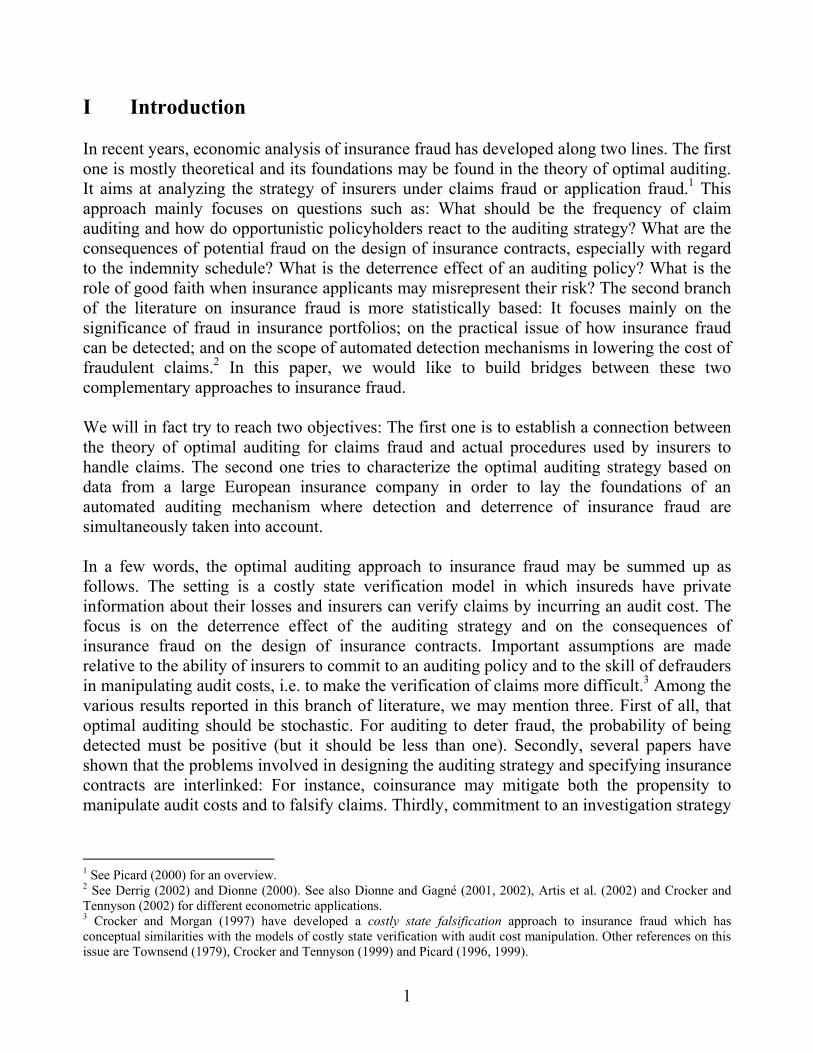
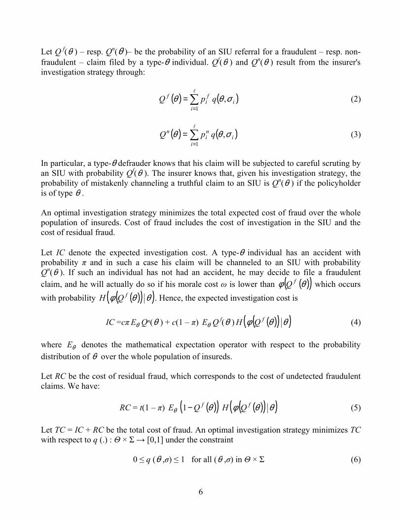
which is the expected cost of fraudulent claims. This cost includes the investigation cost of the claim channeled to an SIU and the cost of paying out unwarranted insurance indemnities. λ(i) and µ(i) are decreasing functions, which implies that Cn(i) and Cf(θ ,i) are respectively decreasing and increasing with respect to i. The optimal investigation strategy trades off excessive auditing of non-fraudulent claims against inadequate deterrence and detection of fraudulent claims. The optimal critical suspicion index i*(θ ) minimizes Cn(i) + Cf(θ ,i) as represented in Figure 1.

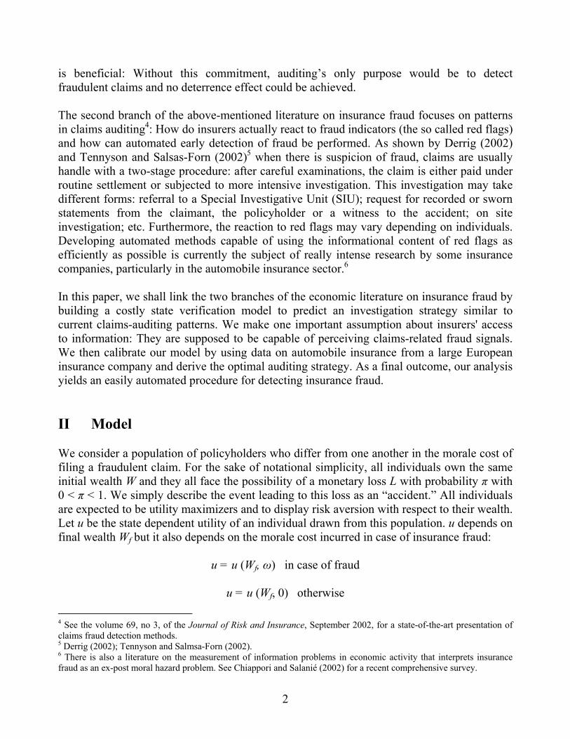
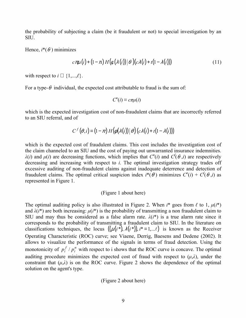
(Figure 1 about here) The optimal auditing policy is also illustrated in Figure 2. When i* goes from ℓ to 1, µ(i*) and λ(i*) are both increasing: µ(i*) is the probability of transmitting a non fraudulent claim to SIU and may thus be considered as a false alarm rate. λ(i*) is a true alarm rate since it corresponds to the probability of transmitting a fraudulent claim to SIU. In the literature on classifications techniques, the locus ( ) ( )( )( )l...,1*,*,* =iii λµ is known as the Receiver Operating Characteristic (ROC) curve; see Viaene, Derrig, Baesens and Dedene (2002). It allows to visualize the performance of the signals in terms of fraud detection. Using the monotonicity of n

if

i pp / with respect to i shows that the ROC curve is concave. The optimal auditing procedure minimizes the expected cost of fraud with respect to (µ,λ), under the constraint that (µ,λ) is on the ROC curve. Figure 2 shows the dependence of the optimal solution on the agent's type.

(Figure 2 about here)

10

Let

( ) ( ) ( )( )θφπθτ QHQ −= 1, and

( ) ( ) ( )( )( )( ) 0

', >=

θφθφφ

θηQH

QhQQQ

τ(Q,θ ) is the fraud rate, i.e. the average number of fraudulent claims for a type-θ insured, when the probability of being detected is equal to Q. Note in particular that τ(Q,θ 0) < τ(Q,θ 1) for all Q, if moving from θ 1 to θ 0, shifts the distribution of ω in the first-order stochastic dominance direction. η(Q,θ 1) is the elasticity of fraud (in absolute value), i.e. the percentage decrease in the fraud rate following a one percent increase in the probability of detection. Proposition 2 says that a higher fraud rate and/or a larger elasticity of fraud should entail more systematic auditing by an SIU. Proposition 2 Assume that A(Q,θ ) = ( ) ( )( )θφ QHQtcQ −+ 1 is convex in Q. If ( )( ) ( )( )0010 ,, θθτθθτ ff QQ ≥ (12) and ( )( ) ( )( )0010 ,, θθηθθη ff QQ ≥ (13) then

( ) ( )01 ** θθ ii ≤ . Proof Assume that A(Q,θ ) is convex in Q. Let 0θ and 1θ in Θ such that (12) and (13) hold. Assume moreover that ( )1* θi > ( )0θ*i , which gives: Qf ( )1θ > Qf ( )0θ (14) Let i ∈ {1,...ℓ} such that:

( ) ( )10 ** θθ iii <≤ . Proposition 1 then gives:

11

( ) 1,0 =iq σθ ( ) 0,1 =iq σθ .

Writing optimality conditions as in the proof of Proposition 1 yields: ( ) ( )( ) 0,1 00

'1 ≤−+ f

ifn

i pQApc θθππ (15) and ( ) ( )( ) 0,1 11

'1 ≥−+ f

ifn

i pQApc θθππ (16) Using (14) and the convexity of Q → A(Q,θ ) gives: ( )( ) ( )( )11

'110

'1 ,, θθθθ ff QAQA > . (17)

(16) and (17) give: ( ) ( )( ) 0,1 10

'1 >−+ f

ifn

i pQApc θθππ . (18) (13) and (16) then imply: ( )( ) ( )( )00

'110

'1 ,, θθθθ ff QAQA > . (19)

We have

( ) ( ) ( )( ) ( ) ( )( ) ( )( )QtcQQhQQHtcQA −++−= 1','1 θφφθφθ

which may be rewritten as:

( ) ( ) ( ) ( )

−++−−

−= θηπθτθ ,1

1,,'

1 QQ

QtcQctQQA

Using (12) and (13) gives

( )( ) ( )( )00'110

'1 ,, θθθθ ff QAQA <

which contradicts (19). Hence, we may conclude that i*(θ 1) ≤ i*(θ 0), which completes the proof. ■ We know that A(Q,θ ) is decreasing in Q, thereby reflecting the fact that increasing the audit probability allows the insurer to cut fraud costs, either directly through the detection of fraudulent claims, or indirectly by deterring fraud. Assuming that A(Q,θ ) is convex in Q

12

means that the marginal benefit of auditing is decreasing. The logic at work in Proposition 2 is the following: Auditing will cut fraud costs all the more efficiently if the insured belongs to a group with a high fraud and/or elasticity rate. Indeed, the higher the fraud rate, the greater the direct benefits auditing provides by detecting fraudulent claims, and the greater the elasticity of fraud, the greater the indirect deterrence effect. If the rate and elasticity of fraud are higher for θ 1 than for θ 0, then, undoubtedly, claims should not receive less scrutiny when they are filed by type-θ 1 than type-θ 0 individuals. In practice (and particularly for the calibration of real data), we may assume that the activity of an SIU is budget-constrained: antifraud expenditures should be less than some (exogenously given) upper limit K, which gives the following additional constraint: ( ) ( ) ( ) ( )( )( ) KQHQEcQEc ffn ≤−+ θθφθπθπ θθ 1 (20) An optimal investigation strategy then minimizes TC with respect to q(.) : Θ × Σ → [0,1] subject to (6) and (20). Proposition 3 shows that the qualitative characterization of the antifraud policy is not affected by the addition of this upper limit on possible investigation expenditures. Proposition 3 Propositions 1 and 2 are still valid when the investigation policy is budget constrained. Proof Let α be a (nonnegative) Kuhn-Tucker multiplier associated with (20) when TC is minimized with respect to q(θ ,σ) subject to (6) and (20). Pointwise minimization gives:

( ) ( ) ( )( )( )( )( )

=≥<==≤

−++0,01,01,0

,~11 '

i

i

if

if

ini

qifqifqif

pQApcσθσθσθ

θθπαπ

where

( ) ( ) ( )( ) ( )( )θφαθ QHQtQcQA −++= 11,~ Proposition 3 can then be proved in the same way as Propositions 1 and 2. ■ Let ( )θσ ,iFP be the probability of fraud depending on the perceived signal and on the type of policyholder. ( )θσ ,iFP is given by (1) with x = ( )θFP ; ( )θFP denotes the probability of fraud for type θ individuals and it is given by:

13

( ) ( ) ( )( )( )( ) ( )( )( )θθφππ

θθφπθ f

f

QHQH

FP−+

−=

11

. (21)

When signal σi is perceived, the expected benefit of an SIU investigation is:

( ) ctFP i −θσ , Proposition 4 shows that the optimal investigation strategy involves transmitting suspicious claims to SIU in cases where the expected benefit of such a special investigation may be negative. Proposition 4 When there is no upper limit on SIU expenditures, the optimal investigation strategy is such that:

( )( )θσ θ ,*iFP t < c for all θ in Θ. Proof We have:

( )( ) ( )( ) ( )( )( ) ( )( )( ) ( )( )( ) ( ) ( )( )( ).

'1,'1

θθφθθφ

θφθθφθθff

fff

QHtcQHtc

QQhQtcqQA

−<−+

−+=

Hence

( ) ( )( ) ( )( ) ( )( )( )θθφπ

πθθπ

πff QHtc

cQA

c−−

−<−

−1,1 '

1 (22)

which gives:10

( )

( ) ( )( ) ( )( )( )θθφππ

θ

θfn

i

fi

QHtcc

p

p

−−−<

1*

* (23)

Using (21), (23) and

10 We here assume that ( ) ( )( ) ( ) ( )( )n

if

ini

fi pppp 1*1*** // −−− θθθθ is small enough for (23) to be implied by (7) and (22).

14

( )

( )

( )( ) ( )( )( ) ( )( )( )θσθ

θσθ

θ

θ

θ

θ

,1

,1

*

*

*

*

i

ini

fi

FPFP

FPFP

p

p

−

−=

gives: ( )( ) ctFP i <θσ θ ,* . ■ Since ( )θσ ,iFP is increasing in i, Proposition 4 means that there exists i**(θ ) larger than i*(θ ) such that:

( )( ) ( )( )tFPctFP ii θσθσ θθ ,, 1**** +<< . Forwarding the claim to an SIU is profitable only if the suspicion index i is larger than i**(θ ). Hence, it is optimal to channel the claim to an SIU when ( ) ( )θθ *** iii ≤≤ , although in such a case the expected profit drawn from investigation is negative. This result follows from the fact that the investigation strategy acts as a deterrent: it dissuades some insureds (those with the highest morale costs) from defrauding. Such a strategy involves a stronger investigation policy than the one that would consist in transferring a claim to an SIU when the direct monetary benefits expected from investigation are positive. The indirect deterrence effects of the investigation policy should also be taken into account, which leads to more frequent investigation. We are now ready to test the main propositions of the article. IV Data The data come from a large insurer in Europe. We draw a sample from the automobile insurance claims files containing information on automobile thefts and collisions. Chart 1 presents the parameters of the original data set. The first group of files (A) comes from the company’s SIU. This is the population of claims referred to this unit over a given period by claims handlers suspecting fraud. Of the 857 files referred to the SIU, 184 contained no fraud and 673 were classified as cases of either established or suspected fraud. As for Belhadji et al. (2000), we considered all these files as fraudulent because they all contained enough evidence of fraud to serve in designing a model for forwarding suspicious files to the SIU. Out of these 673 files, 181 were classified as suspicious because there was not enough evidence or proof to convince the SIU that these claims should not be paid.

(Chart 1 about here) The second group of files (B) was randomly selected from the population of claims that the insurer did not think contained any type of fraud during the same period of time. We chose to

15

select only about 1,000 files in the reference group, because the cost of compiling information on fraud indicators is very high. In fact, to find significant indicators for fraud detection, our assistants had to read each file in groups (A and B) to search for the potential indicators identified by members of the SIU (about 50). Chart 2 describes the breakdown of files chosen for the analysis: the 184 files without any fraud in A were transferred to B yielding two groups of files (A’ with fraud and B’ without fraud) and showing that 37% of the files contained established or suspected fraud.

(Chart 2 about here) In order to obtain a final sample representing the true proportion of fraudulent claims in the company, we used the bootstrapping method. We applied two complementary techniques. The first consisted in replicating the original B’ subsample six times, yielding 6,674 observations (6 × 1,129). Then we took a random sample (with replacement) from these 6,674 observations in order to obtain the additional 953 observations needed to produce a fraud rate of 8%, which is supposed to be the fraud rate in the insurer’s portfolio. The final sample contained 8,400 files, 673 files (A’) containing fraud and 7,727 files (B’’) with no fraud. Chart 3 presents the final sample.

(Chart 3 about here) V Regression Analysis Regression Model An econometric analysis allowed us to identify relevant fraud indicators. We used the standard Logit model for binary choice. The insured has either filed a fraudulent claim or has not. We suppose that the different fraud indicators or individual characteristics in the period studied will affect the status of the file. So we can write:

Prob(Y = Fraud) = F(β’x) and

Prob(Y = No Fraud) = 1 – F(β’x) where x is the vector of explanatory variables (fraud indicators or individual characteristics) and β is the vector of parameters. If we assume that F(·) is the Logistic cumulative distribution function, then we estimate the Logit model. There is no clear evidence that the Logit model is more appropriate than the Probit model for our purpose. Our choice was explained only by mathematical convenience (See Green, 1997, for a longer discussion). Regression Results

16

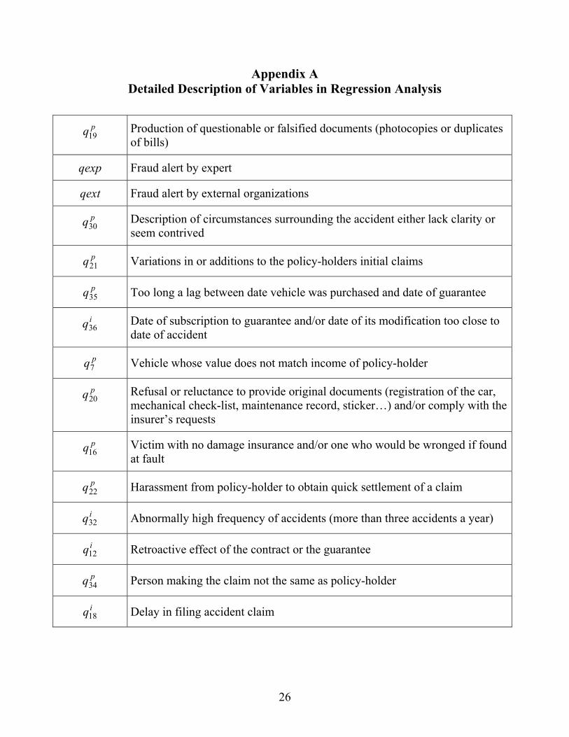
Table 1 reports the regression results. A detailed description of the variables is presented in Appendix A. The first column (without θ variables) in Table 1 is limited to variables identifying fraud indicators. All of them are significant in explaining (positively) the probability that a file may contain either suspected or established fraud at a level of at least 95%. The second column (with θ variables that represent characteristics of policyholders) yields similar results but takes into account two additional variables capable of estimating the probability that a file will be referred to the SIU. As discussed in the theoretical part of the paper, these variables are used to approximate the individual morale cost of fraud. Variables

pq7 and pq16 indicate respectively that owners of vehicles whose value does not match their income and which are not covered by damage insurance are people with a lower morale cost for fraud or a higher probability for filing a fraudulent claim.

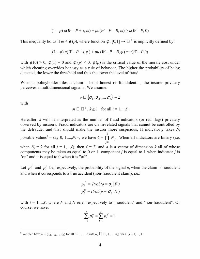
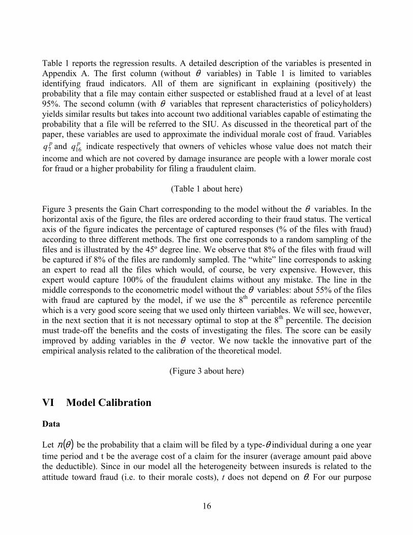
(Table 1 about here) Figure 3 presents the Gain Chart corresponding to the model without the θ variables. In the horizontal axis of the figure, the files are ordered according to their fraud status. The vertical axis of the figure indicates the percentage of captured responses (% of the files with fraud) according to three different methods. The first one corresponds to a random sampling of the files and is illustrated by the 45º degree line. We observe that 8% of the files with fraud will be captured if 8% of the files are randomly sampled. The “white” line corresponds to asking an expert to read all the files which would, of course, be very expensive. However, this expert would capture 100% of the fraudulent claims without any mistake. The line in the middle corresponds to the econometric model without the θ variables: about 55% of the files with fraud are captured by the model, if we use the 8th percentile as reference percentile which is a very good score seeing that we used only thirteen variables. We will see, however, in the next section that it is not necessary optimal to stop at the 8th percentile. The decision must trade-off the benefits and the costs of investigating the files. The score can be easily improved by adding variables in the θ vector. We now tackle the innovative part of the empirical analysis related to the calibration of the theoretical model.

(Figure 3 about here) VI Model Calibration Data Let ( )θπ be the probability that a claim will be filed by a type-θ individual during a one year time period and t be the average cost of a claim for the insurer (average amount paid above the deductible). Since in our model all the heterogeneity between insureds is related to the attitude toward fraud (i.e. to their morale costs), t does not depend on θ. For our purpose

17

( )θπ = 22% and t = 1,284 €. The audit cost c of a claim is equal to 280 € and we already know that the proportion of claims with fraud z(θ) is 8%. Since ( )θπ contains fraudulent claims the accident (theft and collision) probability π is equal to:

( ) ( )( ) %24.201 =− θθπ z Now let ( )( )θλτ ,i be the fraud rate in the insurer portfolio. From equation (11) in Section III,

( )( ) ( ) ( )( )( )θλφπθλτ iHi −= 1, From the above data ( ) ( )θτθτ =,0 can be approximated by:

( ) ( ) ( ) %80.1== θθπθτ z which amounts to assume that the observed current antifraud policy of the company behavior does not incorporate any deterrence effect. For the calibration of the model, we will use the following formula for ( )( )θλτ ,i : ( )( ) ( ) ( )( )γλθτθλτ ii −= 1, (24) where γ is a parameter used to define ( ) ( )( )ii λγλη −−= 1/ , the elasticity of the fraud rate with respect to ( )iλ . Using (24) we can rewrite (11) as: ( ) ( ) ( )( ) ( )( )( )ctitiic −−−+ λλθτπµ γ1 (25)

where ( ) ∑=

=1j

fjpiλ and ( ) ∑

==

1j

njpiµ .

From now on, we assume that θ is given. In other words, the numbers that will be presented below come from the regression without θ . Of course, the analysis can be replicated for different values of θ obtained from the estimation results of the fraud probability, as we will see in the last part of the article. In order to obtain the optimal i by minimizing (25) with respect to i, we must compute the values of ( )iλ and ( )iµ . From (8) and (9) we have:

18

( ) ( )

( ) ( )FPFP

PFPp i

iifi /

/ σσσ==

( )( ) ( )( )[ ] ( )NPFP

PFPp i

iini /

1/1 σσσ

=−

−= .

The conditional probability ( )iFP σ/ can be computed directly from the econometric model.

( )iP σ is much more difficult to obtain directly because the econometric analysis yielded 13 significant fraud indicators and, consequently, 8,192 values for iσ , which are the vectors for fraud measure or signals for fraud. Since our data set is limited to 9,171 observations or files, many potential values for iσ should be nil. We must then use an indirect procedure to compute f

ip and nip . The

procedure below is known in the literature as the simple Bayes classifier method (Viaene et al., 2002) which is equivalent to the Bayes optimal classifier only when all predictors are independent in a given class. It was shown that this simple Bayes classifier often outperforms more powerful classifiers (Duda et al., 2001). From the regression analysis, we know that 13 fraud indicators are significant. qj, j = 1… k, designates the presence ( )1=jq or absence ( )0=jq of the indicator j in a given file. So we can write:

1=ijσ if 1=jq 0=ijσ if 0=jq .

Let the jq be independent given that the file is F or N, we can write:

( )FqobPr jfj /1==α

and ( )NqobPr j

nj /1==α

for j = 1… k, where n

jfj αα > by definition of fraud indicators. The assumption that the qj are

independent given that the file is F or N allows us to write: ( ) ( )f

jj

fjji

fi

ijijFPp αΠαΠσ

σσ−==

==1/

0/1/ (26)

19

( ) ( )njj

njji

ni

ijijNPp αΠαΠσ

σσ−==

==1/

0/1/ (27)

We have now the complete information for model calibration. Results The calibration results are summarized in Table 2. Column 3 presents the computed f

ip from (26) while Column 4 presents the computed n

ip from (27). So we can obtain the ratios ni

fi pp / directly to classify the different σi. Column 1 presents the identification numbers of

the observed σi. They can simply be interpreted as i. One of them will also be the i*. According to Proposition 1, the optimal investigation strategy consists in ranking the observations i by using the values n

if

i pp / in an increasing manner. The corresponding values are in Column 5 of Table 2. Table 2 has 213 = 8.192 lines because the regression analysis identified 13 significant binary indicators. So we obtain 8.192 values for iσ in Column 2 resulting from different combinations of N and Y where N indicates that an indicator is not present and Y indicates that an indicator is present for that line. For example, the first line in Column 2 indicates that no significant fraud indicator is present. Line 2 indicates that only the 8th fraud indicator is present.

(Table 2 about here) Column 6 yields the value of λ(i), the probability of channeling a fraudulent claim to the SIU when the critical index of suspicion is i. In line 1, λ(i) =1 and all claims with fraud are audited by definition because the critical suspicion index is i = 1. However, as we shall see, this strategy will be very costly and will not be optimal. The optimal critical suspicion index, denoted i*, will trade off the benefits and the costs of auditing. Another example would be to choose i = 10 as a critical suspicion index, which means that all files with a ratio n

if

i pp / higher than 0.17 will be audited. This would mean that 95% of the fraudulent claims would be audited and that 45% of the no-fraudulent claims would be audited (µ(i) in column 7). This might also be a very costly strategy. Let us now consider in detail the different auditing costs. Column 8 presents the expected investigation cost of a non-fraudulent claim for different values of µ(i), the probability that a non-fraudulent claim will be channeled to the SIU. So for line one, we have:

280€ × 0.2024 = 56.67€

20

where π = 0.2024 is the accident probability, 280€ is the audit cost and µ(i) = 1. For line 10, this cost is reduced to 25.66€ because µ(i) is equal to 0.45291. Column 9 yields the average cost of fraudulent claims for different values of λ(i) and column 10 computes the expected cost of a fraudulent claim for η = 0 and τ = 0.018. In line 1, this expected cost is very low because it is reduced to 280€ × τ. Moreover, here 0=γ which means that there is no incentive or deterrent effect associated with a variation in λ(i). Column 11 is the sum of columns 8 and 10 and computes the expected total cost of fraud per policyholder. The optimal ( )θ*i will be obtained by minimizing this expected cost. Finally, Columns 12, 13, and 14 give, respectively, information on the audit probability for different values of i, the expected audit cost for different values of i, and the probability of fraud for audited claims, given that we audit all claims having a i > i*. Again, if i* = 1, all claims are audited and the probability of fraud is equal to the average fraud rate in the sample because there is no incentive effect here ( 0=γ ). However, if i* = 10, the auditing strategy will be more focused on claims with suspected fraud (λ(i) = 0.95 and µ(i) = 0.45) and the probability of fraud in audited claims is equal to 0.1544. The optimal solution is at line 238 = i*(θ). Five significant indicators are present at the σ(i*) threshold. λ(i*) = 0.6805, which means that 68% of the fraudulent claims will be audited. So the optimal expected cost of a fraudulent claim in the total insurer portfolio (Column 10) is 10.57€. µ(i*) = 0.04, which means that only 4% of the non-fraudulent claims will be audited. The corresponding optimal expected cost of a non-fraudulent claim in the insurer portfolio is equal to 2.25€. So the optimal expected total cost of fraud reaches its minimal value at 12.83€. Note that the corresponding cost at line 1 (audit all claims) is 61.60€ and that at line 8192 it is 22.56€. The corresponding optimal audit probability is 9.10% of the files (column 12) and the optimal audit cost per claim is 25.50€. Finally,

P(F/i > i*) = ( )( ) ( )( ) *)(1*)(

*)(iziz

izµθλθ

λθ−+

= 59.8%

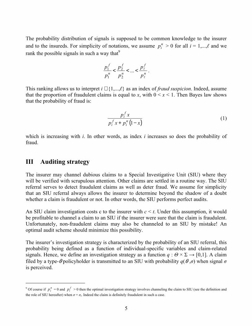
which means that 59.8% of audited claims prove to be fraudulent, which can also be verified in Figure 3 at the 9.10% value. Figure 4 shows how the expected total cost of fraud varies in function of the expected audit cost per claim.

(Figure 4 about here) Table 3 presents different sensibility analyses of the optimal solution in Table 2 with respect to the parameters γ and ( )θz . Remember that ( )θz is the fraud rate in the insurer portfolio. This fraud rate is a function of θ , the morale cost of fraud. Two interpretations are possible: θ can be the average morale cost of fraud in the entire portfolio or the average cost of fraud

21

for a subgroup of policyholders whose characteristics correlate with their true morale cost of fraud, a variable not observable. Up to now, we have taken no account of such variables in the regression results without considering the θ variables. Table 4 proposes four different values of ( )θz computed by using the regression results in Table 1 with respect to the variables pq7 and pq16 that approximate different values of θ .

(Table 3 about here) Indeed, the two variables ( pq7 and pq16 ) were used to approximate different morale costs of fraud. The value 5.88% for ( )θz corresponds to the case were the two variables are not significant which yields the lowest fraud rate in the portfolio. The other value of interest for the sensibility analysis is that obtained when pq16 is significant and pq7 is not. The corresponding value for ( )θz is 9.93%. The two other cases are not considered because their respective numbers of policyholders is too low.

(Table 4 about here) Deterrence effect and profitability of optimal auditing The parameter γ measures the incentive effect of the optimal audit policy. In Table 2, the value of γ was fixed in zero, which means that the setting for the optimal audit policy took no account of the incentive effect of fraud deterrence. However, we have seen that the higher the probability p of being detected, the lower the ϕ(p) threshold and consequently the lower the level of fraud. When γ is positive, auditing expects such a deterrence effect on fraud. Proposition 2 has characterized the relationship between on one side the intensity of this deterrence effect and the fraud rate, and on then other side the optimal auditing strategy. It states that when the function ( )θ,QA is convex in Q or here in ( )iλ , auditing is increasingly successful at reducing fraud costs as the fraud rate rises (higher benefit of auditing) or as the elasticity of fraud grows (higher deterrence or incentive effect). These results are tested directly in Table 4. We observe, for the three different values of the fraud rate ( )θz , that i* decreases (audit increases) when the elasticity of the fraud rate increases (in absolute value) with respect to ( )iλ . This is the deterrence effect: When the insurer announces an audit policy, he increases the threshold ϕ(p) or the critical value of the morale cost under which cheating dominates honesty because the audit probability of defrauders increases. The results of Table 4 also indicate clearly that fraud audit intensifies (reduction of i* and increase in ( )*iλ ) as the fraud rate ( )θz increases. In other words, the benefits of fighting fraud increase as ( )θz increases.

22

In Table 5, we present monetary values related to our results with data from the insurer. As already mentioned, the claims rate (over the whole portfolio) of that insurer is 22%, which represents about 500,000 claims for the corresponding time period. Without the optimal audit policy, the fraud rate is 8%. So 51 million € are paid for fraudulent claims and the total claim cost is 642 M€. Let us now consider the monetary numbers under the optimal auditing policy of Table 2. First, we know that 9.1% of the files will be audited at a cost of 280 €. Secondly, we also know that 68% of the fraudulent claims will be audited and will not receive any insurance coverage. However, 32% of the fraudulent claims would not be audited. The total claim cost net of audit costs will then be equal to 620 M€, a saving of 22 M€. Finally, we show that auditing all claims is not efficient, as suspected. Indeed, auditing all claims will generate a total claim and audit cost of 731 M€, the total claim cost is reduced to 591 M€ but the total audit cost is equal to 140 M€. VII Conclusion This article aimed at making a bridge between the theory of optimal auditing and the actual claims auditing procedures used by insurers. On the theoretical side, we have shown that the optimal random auditing strategy takes the form of a “red flags strategy” which consists in referring claims to SIU when some fraud indicators are observed. The classification of fraud indicators corresponds to an increasing order in the probability of fraud and such a strategy remains optimal if the investigation policy is budget constrained. Furthermore, the auditing policy acts as a deterrence device and in some cases, the (unconstrained) optimal investigation strategy leads to a SIU referral even if the direct expected gain of such a decision is negative. A strong commitment of the firm is thus necessary for such a policy to be fully implemented. On the empirical side, two significant results were tested by using data from a large European insurance company. We were able to compute a critical suspicion index for fraud, providing a threshold above which all claims must be audited. In fact, according to the optimal model, 68% of the fraud claims are audited while only 4% of the no-fraud claims are audited. We showed that if the insurer applies this policy, he will save more than 22 million € (including audit costs), while he was paying 51 M€ for fraudulent claims. These results were obtained under the conservative scenario that all policyholders share the same morale cost of fraud and that the deterrent effect of the optimal strategy is non-existent. We also showed that it is possible to improve these results by using information that allow us to compute different fraud rates i.e. by including in the regression analysis different variables capable of isolating different groups of insureds with different morale costs of fraud. The sensitivity results show that more auditing should be applied to those with higher fraud rates or higher thresholds for the dominance of cheating over honesty. Our numerical results show that the optimal expected audit probability goes from 6.8% to 12.2% when the fraud rate

23

goes from 5.9% (for a low fraud type) to 9.9% (for a high fraud type) which suggests that strongly differentiated audit rates are actually optimal. Finally, our results show how the deterrence effect of the audit scheme can be taken into account and how it affects the optima auditing strategy.

24

References Artis, M., Ayuso, M., Guillén, M. (2002), “Detection of Automobile Insurance Fraud With

Discrete Choice Models and Misclassified Claims,” Journal of Risk and Insurance 69, 3, 325-340.

Belhadji, E.B., Dionne, G., Tarkhani, F. (2000), “A Model for the Detection of Insurance

Fraud,” Geneva Papers on Risk and Insurance Issues and Practice 25, 4, 517-538. Chiappori, P.A., Salanié, B. (forthcoming), “Testing Contract Theory: A Survey of Some

Recent Work,” forthcoming in the Proceedings of the 2000 World Congress of the Econometric Society, Seattle.

Crocker, K.J., Morgan, R.J. (1997), “Is Honesty the Best Policy? Curtailing Insurance Fraud

Through Optimal Incentive Contracts,” Journal of Political Economy 106, 2, 355-375. Crocker, K.J., Tennyson, S. (2002), “Insurance Fraud and Optimal Claims Settlement

Strategies,” Journal of Law and Economics 45, 2, 469-507. Crocker, K.J., Tennyson, S. (1999), “Costly State Falsification or Verification? Theory and

Evidence from Bodily Injury Liability Claims,” in Automobile Insurance: Road Safety, New Drivers, Risks, Insurance Fraud and Regulation, G. Dionne and C. Laberge-Nadeau (Eds), Kluwer Academic Publishers, Boston.

Derrig, R.A. (2002), “Insurance Fraud,” The Journal of Risk and Insurance 69, 3, 271-287. Derrig, R.A., Weisberg, H.I. (2003), “Auto Bodily Injury Claim Settlement in

Massachusetts,” Document, Automobile Insurers Bureau of Massachusetts, 36 p. Dionne, G. (2000), “The Empirical Measure of Information Problems with Emphasis on

Insurance Fraud,” in Handbook of Insurance, G. Dionne (Ed.), Kluwer Academic Publishers, Boston, 395-419.

Dionne, G., Gagné, R. (2002), “Replacement Cost Endorsement and Opportunistic Fraud in

Automobile Insurance,” Journal of Risk and Uncertainty, 213-230. Dionne, G., Gagné, R. (2001), “Deductible Contracts Against Fraudulent Claims: Evidence

from Automobile Insurance,” Review of Economics and Statistics 83, 2, 290-301. Duda, R.O., Hart, P.E., Stork, E.G. (2001), “Pattern Classification,” Wiley, New York. Green, W.H. (1997), Econometric Analysis, Prentice Hall, New Jersey, 1075 pages.

25

Picard, P. (1996), “Auditing Claims in Insurance Market with Fraud: the Credibility Issue,” Journal of Public Economics 63, 27-56.

Picard, P. (2000), “On the Design of Optimal Insurance Contracts Under Manipulation of

Audit Costs,” International Economic Review 41, 4, 1049-1071. Picard, P. (2000), “Economic Analysis of Insurance Fraud,” in Handbook of Insurance, G.

Dionne (Ed.), Kluwer Academic Publishers, Boston, 315-362. Tennyson, S., Salmsa-Forn, P. (2002), “Claims Auditing and Automobile Insurance: Fraud,

Detection and Deterrence Objectives,” The Journal of Risk and Insurance 69, 3, 289-308.

Townsend, R. (1979), “Optimal Contracts and Competitive Markets with Costly State

Verification,” Journal of Economic Theory XXI, 265-293. Viaene, S., Derrig, R.A., Baesens, B., Dedene, G. (2002), “A Comparison of State-of-the-Art

Classification Techniques for Expert Automobile Insurance Claim Fraud Detection,” Journal of Risk and Insurance 69, 3, 373-422.

26

Appendix A Detailed Description of Variables in Regression Analysis

pq19 Production of questionable or falsified documents (photocopies or duplicates

of bills)

qexp Fraud alert by expert

qext Fraud alert by external organizations

pq30 Description of circumstances surrounding the accident either lack clarity or seem contrived

pq21 Variations in or additions to the policy-holders initial claims

pq35 Too long a lag between date vehicle was purchased and date of guarantee

iq36 Date of subscription to guarantee and/or date of its modification too close to date of accident

pq7 Vehicle whose value does not match income of policy-holder

pq20 Refusal or reluctance to provide original documents (registration of the car, mechanical check-list, maintenance record, sticker…) and/or comply with the insurer’s requests

pq16 Victim with no damage insurance and/or one who would be wronged if found at fault

pq22 Harassment from policy-holder to obtain quick settlement of a claim

iq32 Abnormally high frequency of accidents (more than three accidents a year)

iq12 Retroactive effect of the contract or the guarantee

pq34 Person making the claim not the same as policy-holder

iq18 Delay in filing accident claim

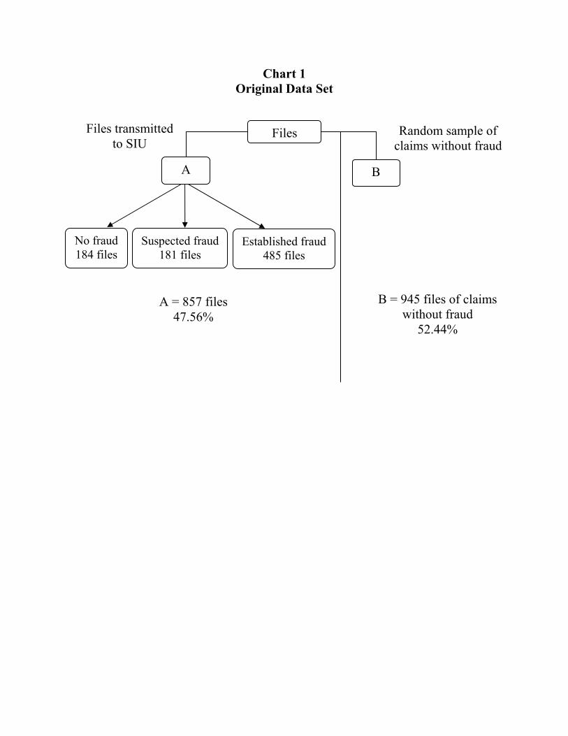
Chart 1 Original Data Set

Files transmitted to SIU

Files

Established fraud485 files

Suspected fraud 181 files

No fraud 184 files

A B

A = 857 files 47.56%

B = 945 files of claimswithout fraud

52.44%

Random sample of claims without fraud

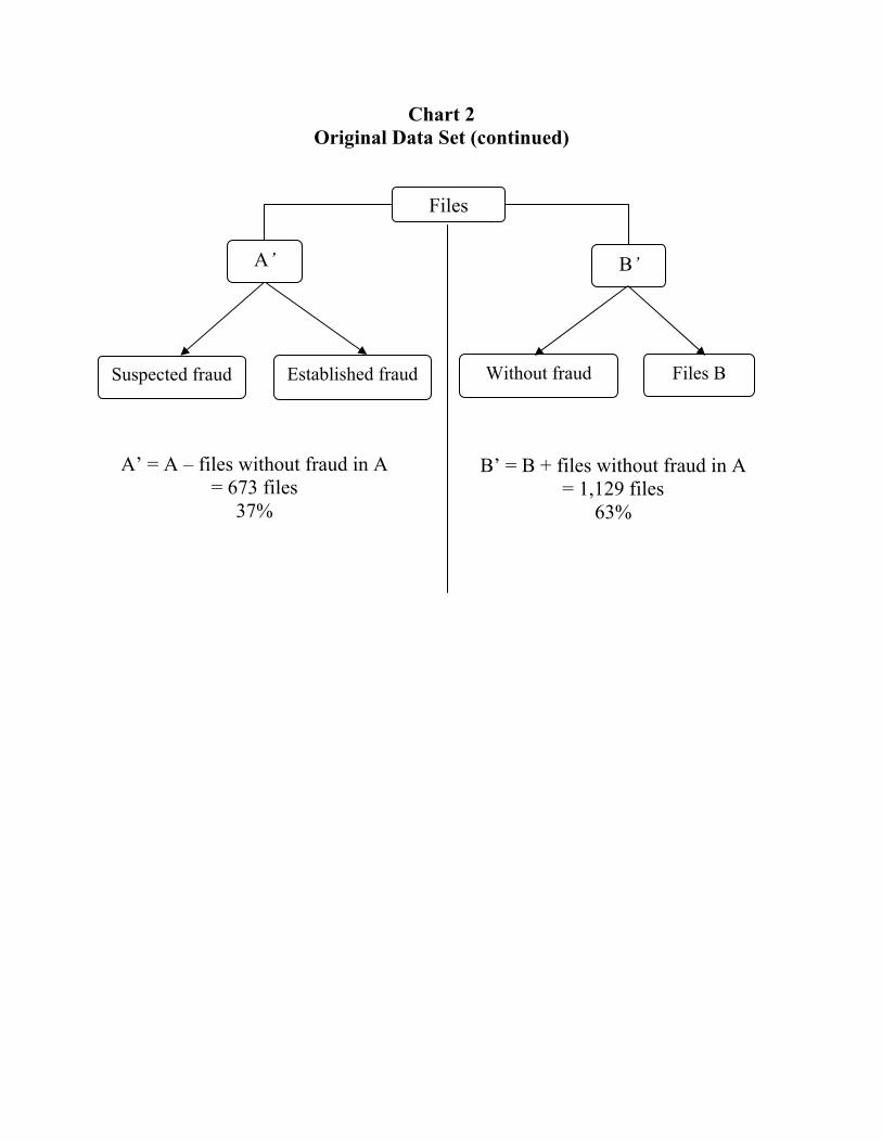
Chart 2 Original Data Set (continued)

Files

A’ B’

Suspected fraud Established fraud Without fraud Files B

B’ = B + files without fraud in A = 1,129 files

63%

A’ = A – files without fraud in A = 673 files

37%

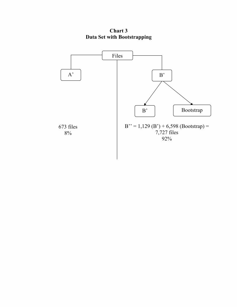
Chart 3 Data Set with Bootstrapping

A’

Bootstrap

B’’ = 1,129 (B’) + 6,598 (Bootstrap) =7,727 files

92%

B’

B’

673 files 8%

Files

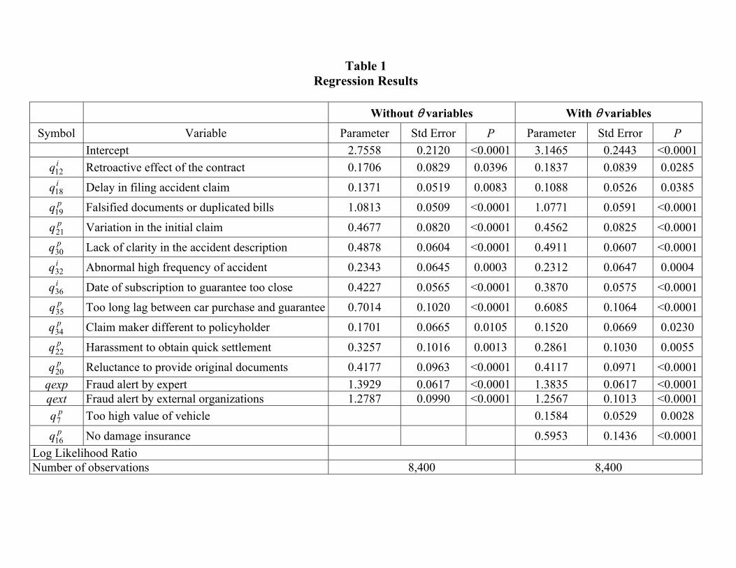
Table 1 Regression Results

Without θ variables With θ variables

Symbol Variable Parameter Std Error P Parameter Std Error P Intercept 2.7558 0.2120 <0.0001 3.1465 0.2443 <0.0001 iq12 Retroactive effect of the contract 0.1706 0.0829 0.0396 0.1837 0.0839 0.0285 iq18 Delay in filing accident claim 0.1371 0.0519 0.0083 0.1088 0.0526 0.0385 pq19 Falsified documents or duplicated bills 1.0813 0.0509 <0.0001 1.0771 0.0591 <0.0001 pq21 Variation in the initial claim 0.4677 0.0820 <0.0001 0.4562 0.0825 <0.0001 pq30 Lack of clarity in the accident description 0.4878 0.0604 <0.0001 0.4911 0.0607 <0.0001 iq32 Abnormal high frequency of accident 0.2343 0.0645 0.0003 0.2312 0.0647 0.0004 iq36 Date of subscription to guarantee too close 0.4227 0.0565 <0.0001 0.3870 0.0575 <0.0001 pq35 Too long lag between car purchase and guarantee 0.7014 0.1020 <0.0001 0.6085 0.1064 <0.0001 pq34 Claim maker different to policyholder 0.1701 0.0665 0.0105 0.1520 0.0669 0.0230 pq22 Harassment to obtain quick settlement 0.3257 0.1016 0.0013 0.2861 0.1030 0.0055 pq20 Reluctance to provide original documents 0.4177 0.0963 <0.0001 0.4117 0.0971 <0.0001

qexp Fraud alert by expert 1.3929 0.0617 <0.0001 1.3835 0.0617 <0.0001 qext Fraud alert by external organizations 1.2787 0.0990 <0.0001 1.2567 0.1013 <0.0001

pq7 Too high value of vehicle 0.1584 0.0529 0.0028 pq16 No damage insurance 0.5953 0.1436 <0.0001

Log Likelihood Ratio Number of observations 8,400 8,400

Table 2 Calibration Results

1 2 3 4 5 6 7 8

i or i* iσ fip n

ip ni

fi pp / ( )iλ ( )iµ ( ) ( )ic µπ=1

1 NNNNNNNNNNNNN 0.01452 0.22967 0.06000 1.00000 1.00000 56.67200 2 NNNNNNNYNNNNN 0.00348 0.03736 0.09000 0.98548 0.77033 43.65614 3 NNNNNNNNNYNNN 0.00424 0.04517 0.09000 0.98201 0.73297 41.53888 4 NNNNNNNNYNNNN 0.01500 0.15222 0.10000 0.97777 0.68780 38.97900 5 NNNNNNNNNNYNN 0.00201 0.01774 0.11000 0.96277 0.53558 30.35239 6 NNNNNNNYNYNNN 0.00101 0.00735 0.14000 0.96075 0.51784 29.34703 7 NNNNNNNYYNNNN 0.00359 0.02476 0.15000 0.95974 0.51049 28.93049 8 NNNNNNNNYYNNN 0.00438 0.02994 0.15000 0.95615 0.48573 27.52729 9 NNNNNNNYNNYNN 0.00048 0.00289 0.17000 0.95177 0.45579 25.83053

10 NNNNNNNNNYYNN 0.00059 0.00349 0.17000 0.95129 0.45291 25.66732 … …

238 NYNYNNNYNYYNN 0.00001 0.00000 3.20000 0.68050 0.03976 2.25328 … …

8192 YYYYYYYYYYYYY 0.00000 0.00000 7567.03000 0.00214 0.00000 0.00000

Table 2 Calibration Results (continued)

9 10 11 12 13 14

( )( )ctit −−λ ( ) ( ) ( )( )( ) ( )( )012 ictit λλθτ −−−= ( ) ( )21 + ( ) ( ) ( ) ( )( ) ( )iziz µθλθ −+= 13 ( )3×c ( )*/ iiFP >

80.00000 4.92800 61.60000 1.00000 280.00000 0.08000 294.57808 5.18457 48.84072 0.78754 220.51176 0.10011 298.06196 5.24589 46.78477 0.75289 210.81010 0.10435 302.31892 5.32081 44.29981 0.71100 199.07933 0.11002 317.37892 5.58587 35.93826 0.56976 159.53146 0.13518 319.40700 5.62156 34.96859 0.55327 154.91638 0.13892 320.42104 5.63941 34.56990 0.54643 153.00040 0.14051 324.02540 5.70285 33.23014 0.52336 146.54181 0.14615 328.42292 5.78024 31.61077 0.49547 138.73115 0.15368 328.90484 5.78873 31.45604 0.49278 137.97851 0.15444

600.77800 10.57369 12.82697 0.09102 25.48538 0.59812

1281.85144 22.56059 22.56059 0.00017 0.04794 1.00000

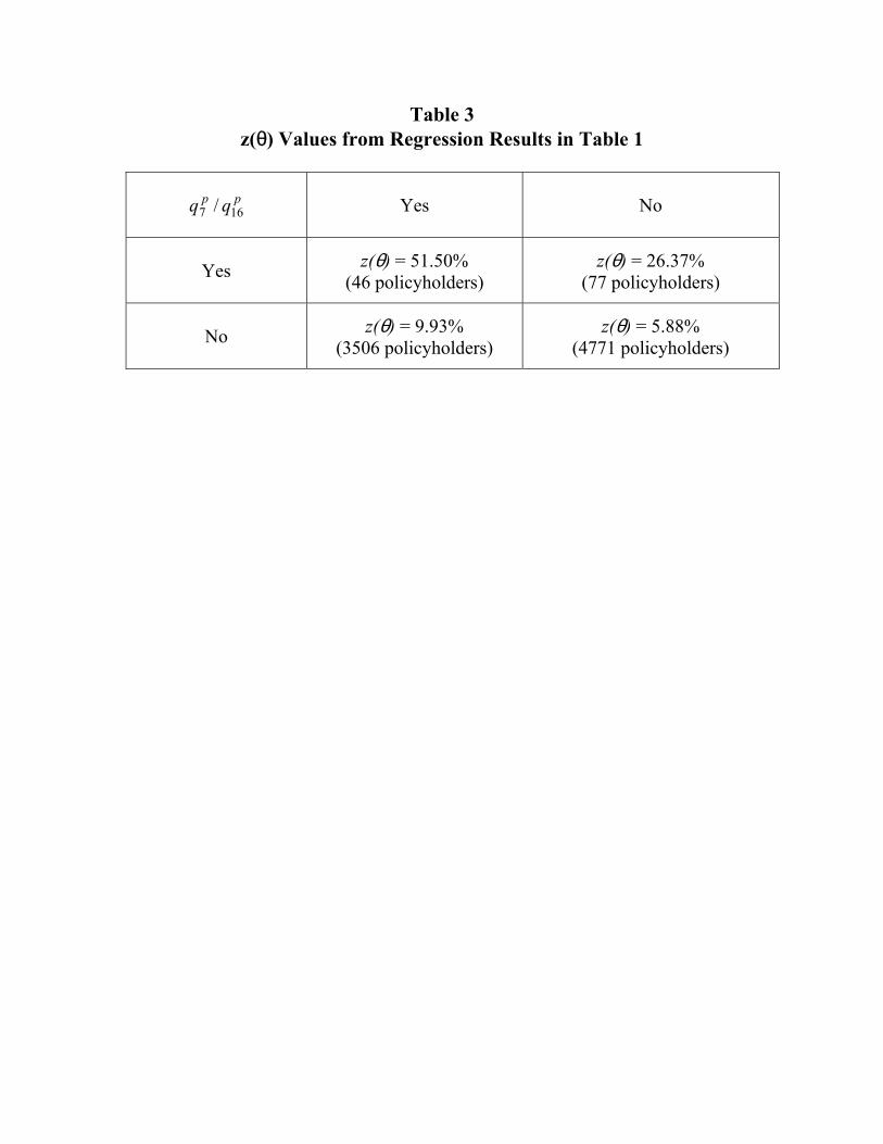
Table 3 z(θ) Values from Regression Results in Table 1

pp qq 167 /

Yes

No

Yes

z(θ) = 51.50% (46 policyholders)

z(θ) = 26.37% (77 policyholders)

No

z(θ) = 9.93% (3506 policyholders)

z(θ) = 5.88% (4771 policyholders)

Table 4 Sensibility of Optimal Solutions With Respect to γ and z(θ)

Case Parameters OptimalTreshold Expected Cost of Fraud Expected Audit

Probability

Audit Probabiliy of Defrauders

z(θ) η(θ)(1) γ π τ(θ) i* τ(θ) (1 - λ(i*))γ (t - λ(i*) (t - c))z(θ) λ(i*) + (1 - z(θ)) µ(i*) λ(i*) A 0.0800 0.00 0.00 0.2024 0.0176 238 12.83 0.0910 0.6805 B 0.0800 0.11 0.05 0.2024 0.0176 232 12.24 0.0952 0.6916 C 0.0800 0.23 0.10 0.2024 0.0176 224 11.68 0.0985 0.7004 D 0.0800 0.82 0.35 0.2024 0.0176 217 9.31 0.0995 0.7030 E 0.0588 0.00 0.00 0.2024 0.0126 304 9.74 0.0676 0.6485 F 0.0588 0.03 0.05 0.2024 0.0126 298 9.34 0.0680 0.6500 G 0.0588 0.19 0.10 0.2024 0.0126 293 8.96 0.0683 0.6509 H 0.0588 0.66 0.35 0.2024 0.0126 279 7.31 0.0693 0.6543 I 0.0993 0.00 0.00 0.2024 0.0242 183 16.62 0.1217 0.7240 J 0.0993 0.14 0.05 0.2024 0.0242 179 15.77 0.1221 0.7248 K 0.0993 0.26 0.10 0.2024 0.0242 179 14.98 0.1221 0.7248 L 0.0993 0.93 0.35 0.2024 0.0242 171 11.72 0.1234 0.7274

(1) η(θ) = -(λ(i*) / 1-(λ(i*)) γ in absolute value.

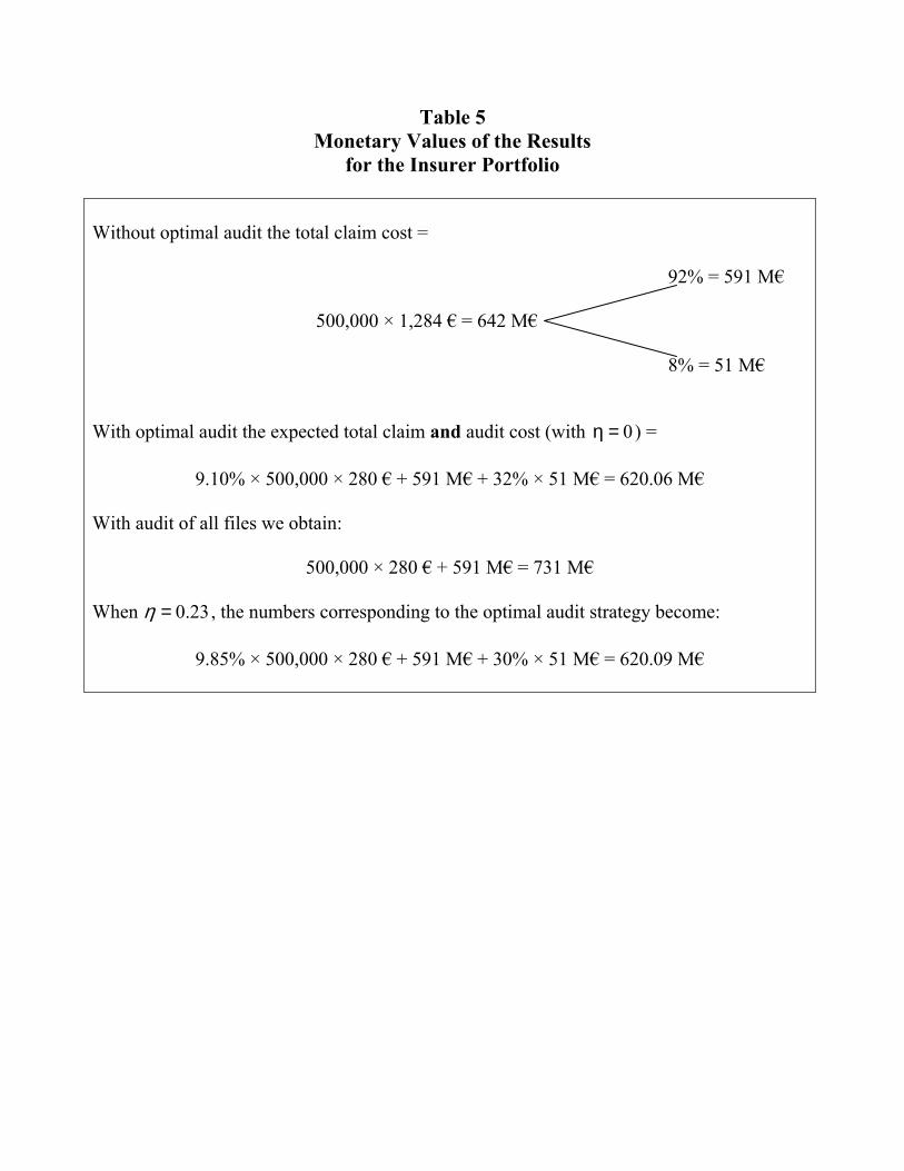
Table 5 Monetary Values of the Results

for the Insurer Portfolio

Without optimal audit the total claim cost = 92% = 591 M€

500,000 × 1,284 € = 642 M€ 8% = 51 M€ With optimal audit the expected total claim and audit cost (with 0=η ) =

9.10% × 500,000 × 280 € + 591 M€ + 32% × 51 M€ = 620.06 M€ With audit of all files we obtain:

500,000 × 280 € + 591 M€ = 731 M€ When 23.0=η , the numbers corresponding to the optimal audit strategy become:

9.85% × 500,000 × 280 € + 591 M€ + 30% × 51 M€ = 620.09 M€

1

Cn(i) Cf(θ,i)

i*(θ) i

Cn(i) + Cf(θ,i)

Figure 1

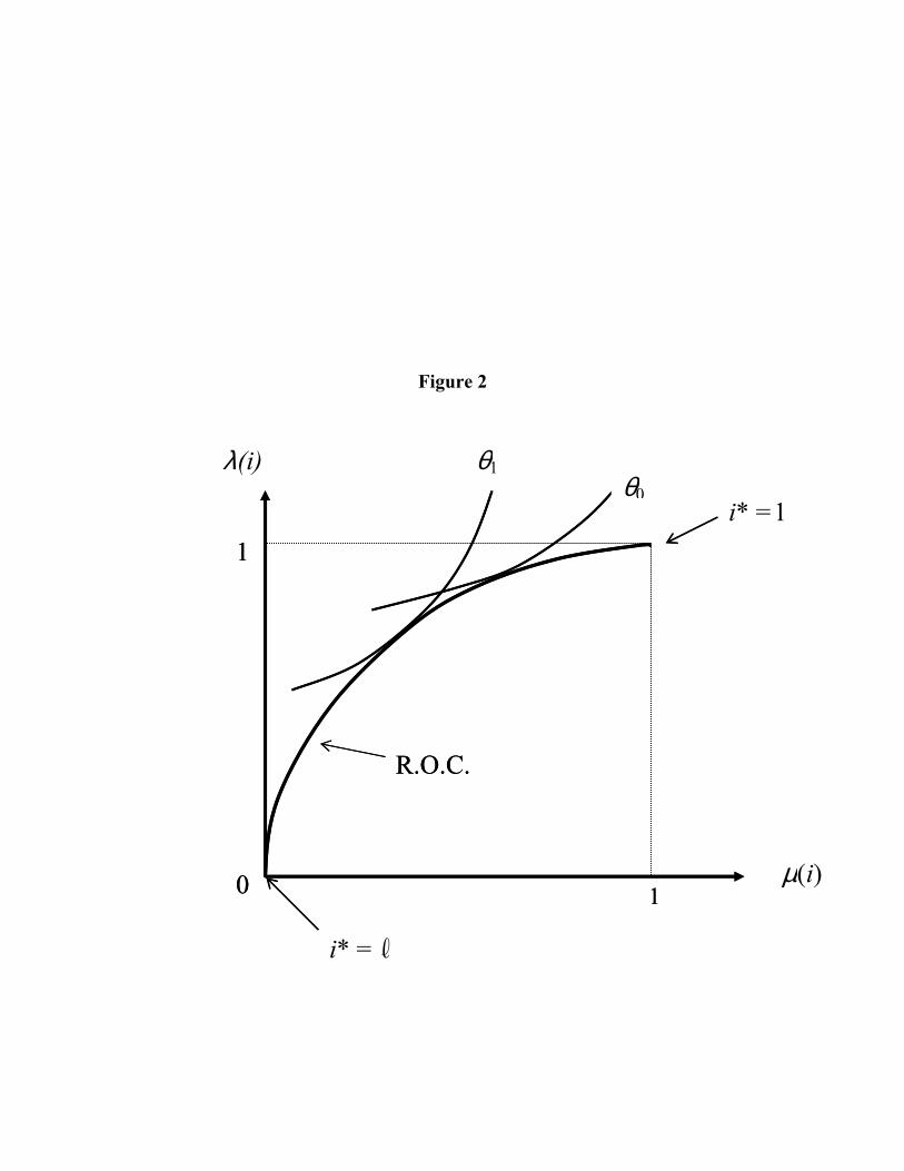
Figure 2

i* =1 θ0

θ1

1 0 µ(i)

λ(i)

1

R.O.C.

i* =

i* =1 θ0

1 0

1

R.O.C.

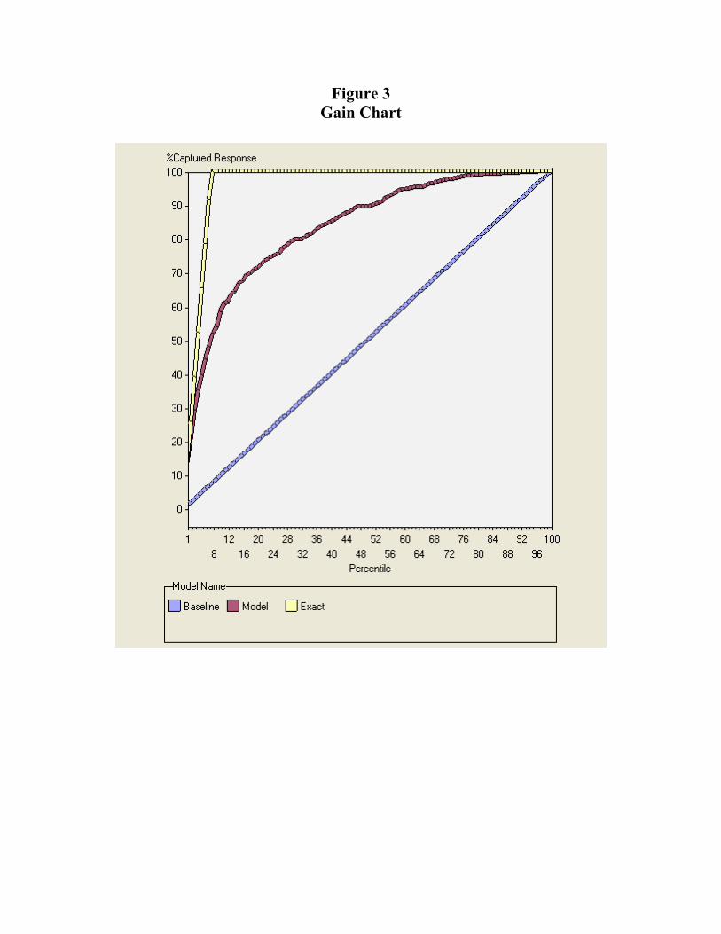
Figure 3 Gain Chart

Figure 4Expected Total Fraud Cost per Insured

0

10

20

30

40

50

60

70

0 20 40 60 80 100

Expected Audit Cost per Claim