OPTICAL OBSERVABLES IN STARS WITH

NON-STATIONARY ATMOSPHERES

R. W. Hillendahl

Science Applications, Inc.

2680 Hanover Street

Palo Alto, California

199

https://ntrs.nasa.gov/search.jsp?R=19800016748 2018-07-15T07:06:44+00:00Z

ABSTRACT

Experience gained by use of cepheid modeling codes to

predict the dimensional and photometric behavior of

nuclear fireballs is used as a means of validating

various computational techniques used in the cepheid

codes. Predicted results from cepheid models are

compared with observations of the continuum and lines

in an effort to demonstrate that the atmospheric

phenomena in cepheids are quite complex but that they

can be quantitatively modeled. It is hoped that the

discussion may provide guidance for cepheid observers.

2OO

INTRODUCTION

The application of the artificial viscDsity technique

(Von Neumann and Richtmyer, 1950) to the explicit

hydrodynamic modeling of spherical systems (Brode,

1955) represents a fundamental milestone in computer

modeling. Subsequently, Brode combined radiative

diffusion with the hydrodynamic motion (Brode, 1956-

1957), having incorporated the implicit Henyey method

(Henyey, Le Levier, Levee, BGhm, and Wilets, 1959)

with the assistance of Le Levier. He then produced

the first radiation-hydrodynamic models of the fire-

ball which results from a nuclear explosion in the

atmosphere (Brode, 1958, 1959a, 1959b). Christy

(Christy, 1964, 1967) later modified the Brode technique

and applied it to his pulsation studies of stellar

envelopes and thus laid the foundation for many sub-

sequent investigations.

During the period where Brode was producing his models

of fireballs, the present author was engaged in making

astrophysical and photgraphic observations of fireballs

(Hillendahl, 1959). This afforded an opportunity for

the quantitative comparison of Brode's modeling tech-

niques with observational data having a much higher

degree of precision than is possible from stellar

observations. The results of such comparisons validated

the hydrodynamic and radiative diffusion techniques used

by Brode, but identified the need for an improved

treatment of the radiative transport in the observable

atmospheric layers. As a student of Henyey, the author

developed a radiation-hydrodynamics technique designed

to treat all regions of the star (Hillendahl, 1962,

201

1964) which was used both for cepheid modeling and in

a relaxation technique (Hillendahl, 1965a) for the

study of stable Henyey models. This "SUPER NOVA" code

was later adapted for use in an extensive study of

fireballs (Hillendahl, 1965b, 1966).

This presentation provides a brief review of selected

numerical and interpretational techniques which have

a proven usefullness, and a description of some

physical processes which the computer models predict

to occur in stellar atmospheres.

202

MODELING TECHNIQUES

It is well established that some features of stellar

models are sensitive to particular details of the

computational technique. For example, the behavior

of a cepheid model employing the artificial viscosity

technique may be dependent upon the formulation used.

One approach to resolving such difficulties is a

careful comparison against data. Another approach is

for a number of modelers to use their codes to model

a well defined test case so that differences due to

computational techniques can be identified. Both

techniques have been used extensively by the fire-

ball modelers (Brode, 1965). Much of this material is

no longer subject to government security restrictions.

The brief exposition given here is intended to allow

the stellar modeling community to benefit from these

findings and to reduce the number of uncertainties

in their models.

Brode (1965) comPared "standard model" calculations

performed by a number of investigators. He demonstrated

conclusively the importance of an accurate equation of

state which includes the relevant dissociation and

ionization processes. He also demonstrated that

equation of state mustmaintain the correctrelation-

ship between the pressure P and internal energy E if

predicted hydrodynamic phenomena are to correspond

to the experimental observations. Thus if curve fits

or data tables are used in the computational model,

care must be taken to see that the correct relationship

between P and E is reproduced. False hydrodynamic

signals may otherwise be produced.

203

The artificial viscosity technique is a useful device

in the treatment of shock discontinuities. The

literature abounds with various versions referred to

as "linear", "quadratic,', "quartic"; various versions

formulated in terms of velocity gradients and/or

compression ratios; and various recommended values for

the damping constant. Many of these have proven to

be applicable over limited ranges of the variables or

only under limited circumstances. The formulation

discussed by Richtmyer (Richtmyer and Morton, 1967,

page 319) has been shown (Hillendahl, 1965b) to

accurately (±2%) reproduce, without adjustment, the

shock front properties in a nuclear fireball while the

shock pressure changes some six orders of magnitude.

Furthermore, the shock structure produced by the model

satisfies the Rankine-Hugeniot conditions to a high

degree of accuracy. One has no reason to expect that

the Richtmyer formulation would not perform equally

well in stellar calculations.

A useful technique for locating shock fronts and related

phenomena at a given epoch is a listing of the quantity

Q/P as a function of mass or radius, where Q is the arti-

ficial pressure and P is the gas pressure. Non-zero

values, which indicate a compression of the gas, are

then easily identified. The largest value of Q/P

occurs as the shock front is in the process of trans-

versing a given zone. This behavior has been employed

as a shock locator (Simpson, 1973) and as a print control

to cause the radial structure to be displayed at the

instant the shock compression of a given zone is complete.

204

In a model using the artificial viscosity technique,

the Rankine-Hugeniot conditions are satisfied on a time

averaged basis, but not always on an instantaneous

basis. Use of the Simpson technique automatically

selects epochs when these conditions are satisfied

and make the data analysis process simpler.

In the interest of conserving computer time, most modern

codes employ continuously variable time steps chosen

to satisfy various hydrodynamic, radiative; or energetic

criteria. With this capability available, the last

time step during compression of the zone can be chosen

so as to cause a print-out precisely at the end of the

compression of the zone in question. The effects of

finite zoning upon the time history of the shock

location and the shock properties are then minimized.

Use of the artificial viscosity technique results in

a compression of the material ahead of the true shock

front. This compression results also in a false

temperature rise. At temperatures lower than about

15,000°K, the absorption coefficient of the gas is

very temperature dependent (~T9) and the artificial

compression can thus result in the creation of false

optical properties ahead of the shock. Under conditions

where the pre,shock gas would be transparent, and the

post-shock gas opaque, an artificial photosphere will

will be created having a temperature lower, than the

post-shock temperature. The emergent flux is then

depressed. Thus a sudden depression in the computed

light output of a cepheid model may be associated

with the emergence of a shock wave.

205

Two aspects of this distortion of the temperature

profile by the artificial viscosity are of interest.

Simpson (1973) conducted numerical experiments on

fireball shock waves in which he artificially increased

the opacity by a factor of l06. When the post-shock

temperature was below 10_°K, he found that this opacity

increase had a negligible effect upon the temperature

and density profiles because the radiative transfer

could not compete with the hydrodynamics at lower tem-

peratures. It is clear, however, that the false com-

pression due to the artificial viscosity does affect

the radial heat flow, but only in a transient manner.

By separately printing out the hydrodynamic and

radiative terms of the energy equation, one can assess

their relative importance and also to determine whether

a particular configuration exists long enough to result

in a distortion of the temperature profile. This type

of distortion has not proven to be important if the

zone structure if fine enough to meet the other

requirements of goodmodeling.

If one desires to obtain high quality optical output

as a shock wave emerges through the photosphere, it

may be necessary to correct the distorted regions of

the temperature, density, and velocity profiles.

The quantity Q/p described above is very useful in

controlling this process. When the artificial pressure

is small compared to the gas pressure, no correction

is needed. When corrections are needed, the "distorted"

values are temporarily stored so that they can be

206

recovered in order to proceed with the pulsation

model. Substitute values are then used to compute

the observable properties at the epoch in question.

Some investigators, e.g., C. G. Davis (LASL), prefer

not to interrupt the:main calculation. They store

the configuration at epochsof interst for later

"snap-shot" light output calculations.

The estimation of these corrected values is relatively

easy in fireball modeling as the profiles ahead of the

shock are usually known. Twotechniques have been

used in cepheid modeling: space extrapolation and time

extrapolation. Inboth techniques data prior to the

artificial viscosity distortion are used to predict

the needed substitute values. The choice between

the two methods is made on the basis of the slowest

rate of change of the zone properties in either time

or space.

The appearance of a region where Q/P is greater than

zero may not indicate the presence of a shock front.

If the disturbance moves toward a region of lower

pressure it is likely to be a shock wave. If the

disturbance moves toward a region of higher pressure,

it may be an unloading or rarefaction wave. The optical

Properties of various waves arediscussed below.

Because of the demonstrated inability of radiative

diffusion techniques to adequately reproducethe optical

observables from nuclear fireballs, it is to be expected

that such techniques would also have similar deficiencies

when applied to the atmospheres pulsating stars. Here

one is faced with the classical problem of radiative

207

transfer, i.e., the equation of transfer of radiation

describes change in the intensity for a given radiation

frequency and along a given direction in space. To obtain

the radiative flux divergence it is necessary to inte-

grate over both the frequency and over all directions

in space. One approach is to use a large number of

rays at various angles and a large number of radiation

frequencies. One fireball code employing this approach

used about 250 hours of machine time to model the

equivalent of one period of a star. The SUPER NOVA

technique (Hillendahl, 1964, 1965) produced virtually

indistinguishable results and utilized only about 1

hour of machine time (about 5 minutes equivalent

CDC 7600 time). In this technique, the source function

is expanded in a Taylor series, in terms of optical

distance, centered on each zone boundary. An integral

formulation of the equation of transfer is applied to

the finite zone configuration in an equivalent ray

approximation. This results indirect and chord

transmission terms, and in a series of emission terms.

In the optically thin extreme, _ the zero order emission

term reproduces the Planck approximation. In the

optically thick extreme, the first order term reproduces

the Rosseland approximation. Higher order terms are

truncated. The formulation leads to a novel technique

for spectral averaging that is a finite zone equivalent

of the Chandrasekhar or flux weighted mean.

An important feature of this formulation is that it

provides a reasonably high order solution to the well

known problem in cepheid modeling in which the opacity

increases very rapidly at the photosphere causing one

zone to be very optically thick and the next exterior

208'

zone to be nearly transparent. This difficulty

arises when a Rosseland mean or equivalent opacity

approximation is used in which the opacity of a zone

depends only upon the local temperature. The zone

exterior to the photosphere has a low temperature and

thus a low opacity. It cannot absorb radiation and

must depend upon hydrodynamic compression to heat

it sufficiently to increase its opacity so that the

absorption of outward flowing radiation can begin.

The SUPER NOVA formulation employs transmission func-

tions for the outwardly directed radiation which are

of the form

Bx(Ts) exp(-_l£)dl' _. .

T =

f Bx(Ts) dlX

wehre T is the outward transmission

£ is the zone thickness along the characteristic

ray

Ts is the temperature of the next interior zone

Bx is the Planck functionX is the wavelength

UX is the local spectral absorption coefficientand is a function of the local gas density and

temperature.

209

In common with the Planck and Rosseland means, the

transmission function depends upon the local temperature

and density of the gas. But it also depends upon the

zone thickness and temperature of the "source" zone.

It is therefore a function of four variables instead of

two.

In practice these functions are computed in great

detail in a preliminary calculation from detailed

spectral absorption coefficient codes. Because of

the existence of absorption edges, and because the

Planck distribution is a function of AT, it is con-

venient to index these precomputed data in terms of Ts

and Az' where Ts is a property of the source zone and Azdepends only on the properties of the zone whose trans-

mission is desired. This affords a reduction in com-

plexity which makes the method workable.

Other investigators have used the Rosseland approxi-

mation in the interior and a finite number of spectral

bands in and exterlor'to the photosphere. Both of

these methods provide for the non-gray radiative

heating of the gas prior to shockcompression which

cannot be accounted for with an unmodified diffusion

approximation. With the great increase in computer

capabilities since the SUPER NOVAtechnique was

developed, the later technique is probably to be pre-

ferred because less effort is involved when the chemical

Composition is changed.

210

ATMOSPHERIC OBSERVABLES'

The fireball from a nuclear explosion is a relatively

simple object in the astrophysical sense. If one

considers only relatively high energy explosions, then

the nuclear device simply causes the formation of a

hot isothermal sphere of air and exerts no significant

influence on the subsequent hydrodynamic and radiative

development which follows. Even so, this relatively

simple object exhibits a great deal of structure

involving periods of radiative growth, the formation

of shocks, hydrodynamic growth, rarefaction waves,

radiative coolingwaves, dissociation fronts that mimic

H II regions, absorption shells, and similar phenomena.

Pulsating stars are much more complex objects than

fireballs because the gas ahead of the expanding shock

front is not of uniform density. One would, therefore,

expect that the atmospheric phenomena might be even

more complex than in the fireball.

In the case of the fireball, the author (Hillendahl 1966)

demonstrated the capability of the SUPER NOVA cepheid

modeling code (as modified for air) to quantitatively

model the atmospheric phenomena which occur in fireballs.

Both the hydrodynamic and radiative phenomena predicted

by the code are verified by photographic and photometric

measurements. If the same modeling techniques are used

on a cepheid, what type of atmospheric phenomena are

predicted? Can any or all of these phenomena be

confirmed by observation?

211

In an attempt to answer these questions, a number of

models of a 7.6 day cepheid were computed and analyzed

using analysis techniques developed from fireball

experience. The model consisted of a periodic envelope

model supplied by Christy (1968) to which an extended

atmosphere was appended. The augmented models remain

periodic in the denser envelope regions, but never

reach a completely repetitive behavior in the extreme

outer layers where mass :loss is predicted to occur

(Hillendahl 1970). The physical phenomena discussed

below are not dependent upon the precise periodic

behavior of the star.

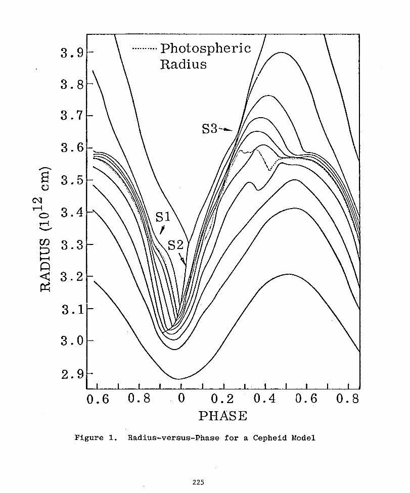
Figure I shows the radius-time history of every fifth

mass point in the computed model. Although several

shock fronts (S1, $2, $3) have been labeled, it is

clear that little, if any, detailed information can

be obtained or illustrated on such' a radius-time display.

Figure 2 shows the same model displayed in a different

fashion. Various shock fronts and rarefaction waves

which have been identified are labeledS and R,

respectively. The photosphere (T=l) has been indicated

by the continuous line.

For a shock front to be observable in continuum light,

it must occupy the photosphericJregion of the star.

In the model shown, the thickness of the photosphere is

from 1 to 2 mass zones throughout the cycle. Thus,

the model predicts that shock waves, including the very

strong shock $2 which "drives" the pulsation, Will

occupy the photosphere only for very brief intervals

in time, i.e., of the order of I-3 hours in a 7-day cepheld.

212

Since the cepheid light curve rises over a time interval

of several'days, it is clear that the light being

observed is not being emitted by the shock front itself.

In the nuclear fireball, the rapid rise in the light

curve, which follows after the expanding shock becomes

transparent, results from the rapid density decrease

on the back side of the shock front. Interior to the

shock front, the densitydecreases rapidly in the

inward direction, while the temperature rfses rapidly

so as to maintaina nearly constant pressure behind

the shock. Just after shock transparency, the photo-

sphere resides in a layer of gas just behind the shock

front. As the whole system expands radially, the

density at every point on the back of the shock

decreases with time in order to conserve mass. This

decrease in density lowers the opacity of the photo-

spheric layer and causes thephotosphere to progress

inward in terms of mass and toward regions of higher

temperature. Since the opacity depends strongly on

the temperature and weakly on the density, only a

slight increase in temperature is needed to compensate

for the density decrease. Thus, the photosphere moves

inward relatively slowly in terms of the mass coordinate,

and actually moves outward in terms of radius.

During rising light in the fireball, the radius of the

photosphere increases by about a factor of two., while

the light'output may increase a factor of 50 or more.

It is clearly the increase in temperature which is

responsible for most of the light increase. This

being the case, one expects, and observes, a larger

213

amplitude for wavelengths to the short wavelength side

of the maximum of the Planck function, i.e., the

amplitude is larger in blue light just as in the

cepheid.

The model calculations predict that the same mechanism

operates during the rising light phases in a cepheid.

During these phases, the models predict an abrupt

spatial density decrease on the back side of the shock

front. If one follows a given shock as it emerges

from deep in the star, it is found that the density

profile behind the shock changes rapidly with radius.

In most regions of the star, the density minimum

behind the shock is only about 30% below the shock

front density. However, when the gas undergoes thermal

ionization as it crosses the shock, the density minimum

is as much as a factor of l0 lower than the shock front

density. This phenomenon is easily explained. The

ionization increases the number of particles and hence

the gas pressure. The increased pressure forces the

gas to expand thus lowering its density.

Clearly then, the amplitude of the light curve depends

upon the magnitude of the density decrease behind the

shock, which in turn depends upon the shock compression

to dissociate or ionize the gas. One would, therefore,

expect pulsating stars to be highly visible if an

ionization or dissociation zone happens to occur near

the photospheric layers. Estimates of the light

amplitude caused by shock emergence when ionization is

not present are of the order of 0.1 mag. (Hillendahl 1969).

214

Because of the real possibility that considerations

such as these might contribute to an observational

selection bias, further investigation seems to be

indicated.

Maximum light (phase 0.0) in the cepheid apparently

occurs when the photosphere has progressed down the

back side of the shock density profile and arrives at

the density minimum. The previously discussed process

responsible for rising light is then interrupted. The

model calculations then indicate an unloading or

rarefaction wave then dominates the atmospheric

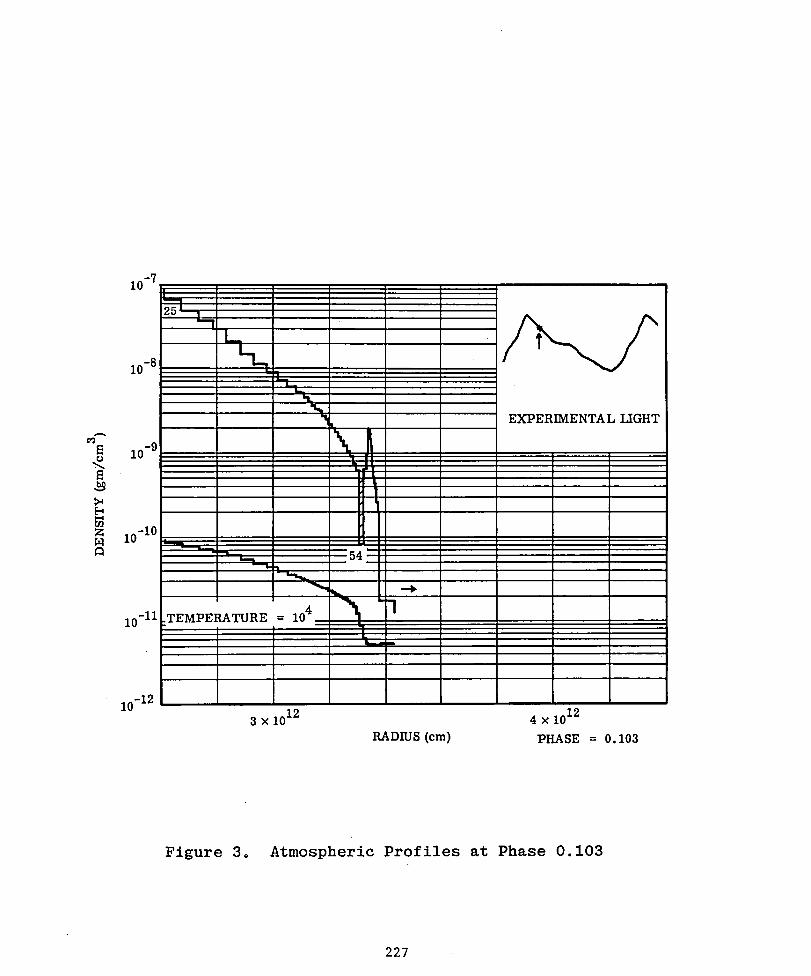
phenomena (Hillendahl 1969, 1970). Figure 3 shows the

density and temperature profiles at phase 0.10S during

the rarefaction wave R2 (see Fig. 2). The density

spike shown is not the shock wave, which has traversed

the atmosphere, but is a residual structure resulting

from the previously described series of events. The

i0-I0 -Sdensity minimum has a value of 5 x gm cm . The

dashed box labeled "54" is a graphical device for

denoting the mass zone in which the photosphere occurs.

Its width is that of the mass zone and its height is a

factor of 6. Graphs similar to Figure 3 have been used

to construct a 16 mm movie which shows the atmospheric

structure throughout the entire period.

The strange atmospheric profiles shown in Figure 3

provided the nucleus for an idea for the construction

of "dynamic" model atmospheres (Hillendahl 1968) for

cepheids. The temperature external to the photosphere

is practically uniform, while the density profile is

slab-like in appearance. Since the absorption

215

!

coefficient depends strongly on the temperature and

weakly on the density, the profile was approximated by

a slab of uniform temperature and density overlying a

blackbody photosphere.

Using a very detailed code for computing the spectral

absorption coefficients, simple models were constructed

using the photospheric temperature Tb and the slab

temperature Ta, density Pa' and thickness Ax asvariable parameters (Hillendahl 1968). Table 1 shows

the results obtained using the "dynamic" model technique

to match the spectral scanner data (Oke 1961) for

Eta Aquilae. Outside the Balmer line blanketed region,

the agreement is relatively good at all but a few

wavelengths. The same technique was applied indiscrim-

inately at all phases with the results shown in Table 2.

At 14 of the 20 phases, the results are quite good.

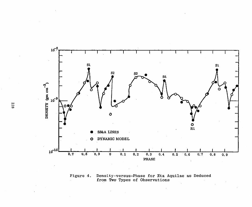
Figure 4 shows the density of the semi-transparent slab

as a function of phase and also the densities obtained

by Fe line analysis (Schwarzschild, et al, 1948). Note

the relatively good agreement and also the amount of

detail. The shock and rarefaction labels correspond

to those on the model results in Figure 2. One would

expect to see a transient density increase after each

shock wave emerges. Figure 4 appears to confirm this

expectation.

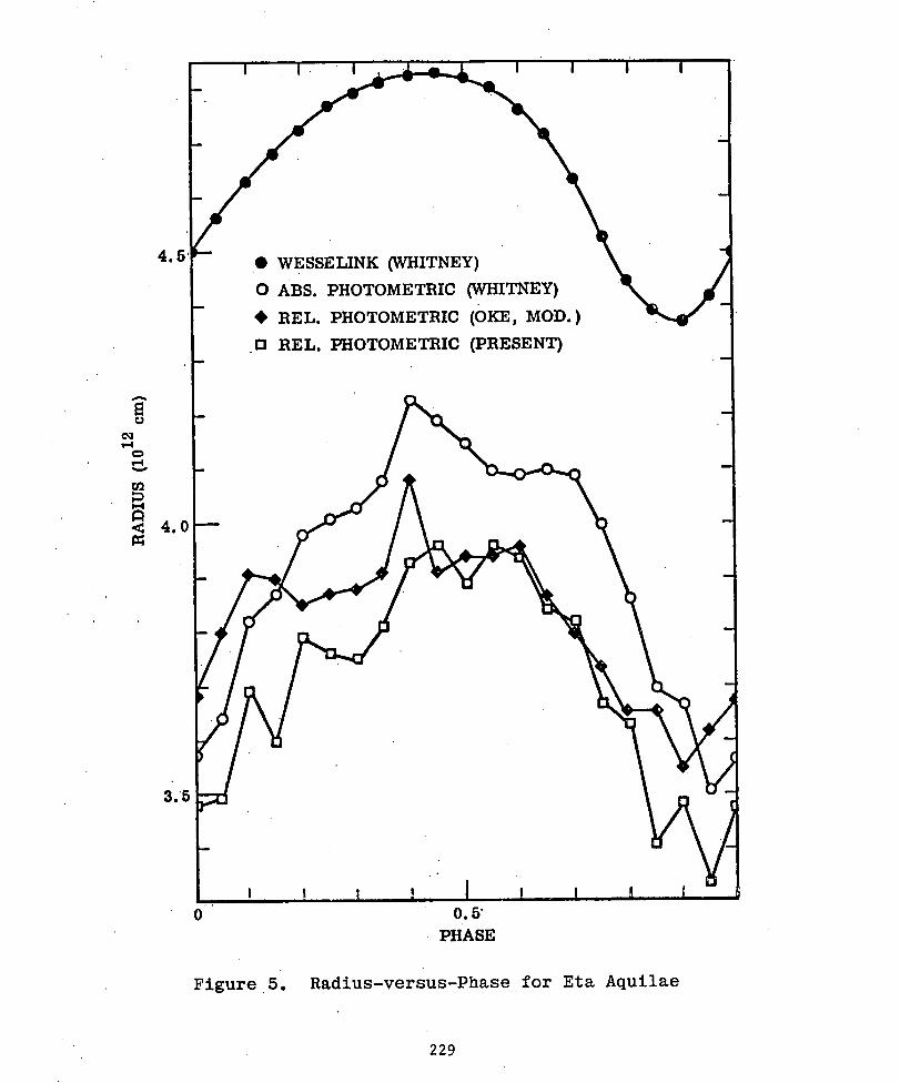
The dynamic atmosphere technique also yields the relative

radius as a function of phase. An absolute normaliza-

tion of the radius can be obtained by two methods

(Hillendahl 1968). The results of this analysis are

216

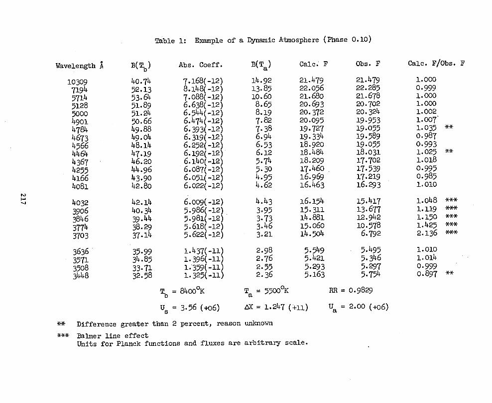
Table l: Example of a Dynamic Atmosphere (Phase O.lO)

Wavelength A B(_) Abs. Coeff. B(Ta) Calc. F Obs. F Calc. F/Obs. F

10309 40.74 7.168(-12) 14.92 21.479 el.479 1.ooo7194 52.13 8.148(-12) 13.85 22.056 22.285 O.9995714 53.64 7.088(-12) i0.6O 21.68O 21.678 i.0005128 51.89 6.638(-12) 8.65 20.693 20.702 i.0005000 51.24 6.544(-12) 8.19 20.372 20.324 i.0024901 50.66 6.474(-12) 7.82 20.095 19.953 i.0074784 49.88 6.393(-12) 7.38 19.727 19.055 i.035 **4673 49.04 6.319(-12) 6.94 19.334 19.589 O.9874566 48.14 6.252(-12) 6.53 18.920 19.055 O.9934464 47.19 6.192(-12) 6.12 18.484 18.031 1.025 _-_4367 46.20 6.140(-12) 5.74 18.209 17.702 i.0184255 44.96 6.087(-12) 5.30 17.460 17.539 O.9954166 43.90 6.051(-12) 4.95 16.969 17.219 0.9854o81 42.8o 6.022(-12) 4.62 16.463 16.293 1.010

4032 42.14 6.009(-12) 4.43 16.154 15.417 i.048 ***3906 40.34 5.986(-12) 3.95 15.311 13.677 1.1193846 39.44 5.981(-12) 3.73 14.881 12.942 i.150 ***3774 38.29 5.618(-12) 3.46 15.060 i0.578 i.425 ***3703 37.14 5.622(-12) 3.21 14.5o4 6.792 2.136 ***

3636 35.99 i.437(-ii) 2.98 5.549 5.495 i.0103571 34.85 i.396(-ii) 2.76 5.421 5.346 1.0143508 33.71 i.•359(-ll) 2.55 5.293 5.297 o.9993448 32.58 1.325(-11) 2.36 5.163 5.754 o.897 *_

= 8400°K Ta = 5500°K RR = 0.9829

Us = 3.56 (+06) AX = 1.247 (.Ii) U = 2.00 (+06)

** Difference greater than 2 percent, reason unknown

*** Balmer line effectUnits for Planck functions and fluxes are arbitrary scale.

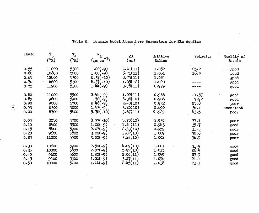
Table 2: Dynamic Model Atmosphere Parameters for Eta Aquilae

Phase Tb T Pa a Z_X Relative Velocity Quality of(OK) (OK) (gm cm-3) (cm) Radius Result

0.59 llO00 5300 1.20(-9) 4.41(11) 1.052 25.2 goodO.60 10800 5200 i.00(-9) 6.71(ii) i.091 16.9 good0.65 128oo 93oo 8.37(-lO) 8.75(zz) 1.o24 goodO.70 166OO 5300 8.37(-lO) 1.05(12) 1.020 good0.79 11900 5300 1.44(-9) 3.78(11) 0.979 good

o. 8o 11o00 5500 2.48(-9) l. o2(ll) o. 966 -l. 97 goodo. 89 9600 59oo 1.72(-9) 6.36(io) 0.908 7.92 good0.90 9000 57O0 2.48(-9) 3.40(10) 0.932 25.8 poor0.95 8300 5800 1.43(-9) 3.20(10) 0.890 36.4 excellentco

o.co 87oo 54oo 5.78(-io) 3.67(ii) o.929 43.5 poor

0.05 8050 9700 8.37(-10) 9.70(10) 0.930 37.1 poorO.i0 8400 5500 l. 00( -9 ) i. 24(11) O.983 35.7 good0.15 8400 9900 2.07(-9) 2.93(10) 0.999 31.3 poorO. 20 9600 5800 3.00(-9) 3.02(i0) i. 009 32.6 pooro.29 11000 59o0 3.00(-9) 3.24(10) 1.002 36.5 poor

0.30 10600 _900 2._0(-9) 4.09(10) 1.001 31.9 goodo. 35 lOOOO 58o0 2.o7(-9) 5.92(lO) i. 015 26.4 good0.40 9600 5600 1.20(-9) 2.00(11) 1.049 23.5 good

O.45 9400 5300 i. 20(-9) 3-27(ii) i. 096 21.1 good0.9O i0000 9400 1.44(-9) 2.45(11) 1.038 23.1 good

compared with other results (Whitney 1955) for

Eta Aquilae in Figure 5.

The method of dynamic atmospheres.should not be inter-

preted as a theoretical modeling technique, but rather

as a means of interpreting observations of the stellar

continuum. The agreement obtained for Eta Aquilae

apparently occurs since hydrodynamic motion is respon-

sible for the creation of the atmospheric profiles.

Numerous attempts to fit the observed continuum from

cepheids with radiative equilibrium model atmospheres

have not proven successful over the entire width of

the observed spectrum.

The cepheid models computed with the SUPER NOVA code

also predict some interesting results relative to the

line spectra from cepheids. During the first half of

the period, when rarefaction waves dominate the atmos-

phere (Fig. 2), the atmospheres exhibit a large velocity

gradient in which the particle velocity within the

unloading region increases almost linearly with radius.

Such a velocity gradient should have an observable

effect on the shapes of spectral lines formed in this

region of the star.

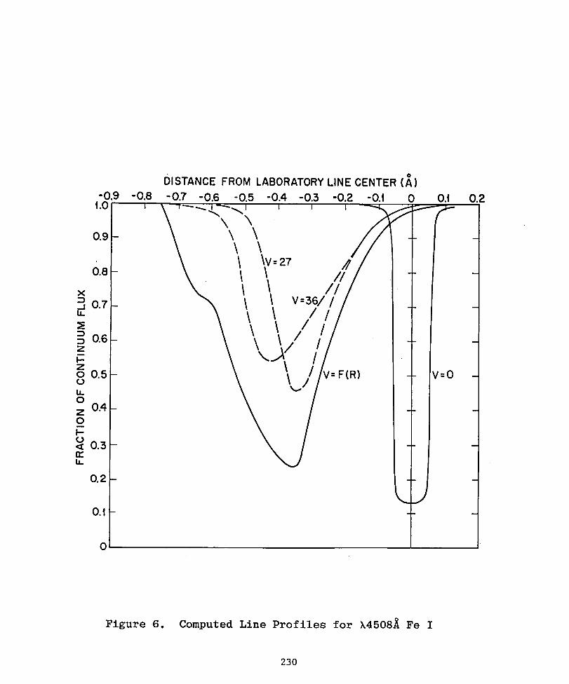
Line profiles have been computed (Hillendahl 1969) from

the atmospheric profiles produced by the SUPER NOVA

code. Figure 6 shows the computed profile for the

4508 _ line of Fe II and is labeled V=F(R). Other

profiles shown were obtained by numerical experimenta-

tion in which the velocity was set to various constant

values throughout the atmosphere.

219

In the computed profile, the velocity distribution is

seen to produce an asymmetry in the line and to approx-

imately double the equivalent width. A satellite line

is obtained at approximately twice the Doppler shift

of the main line. This results from velocity doubling

in the unloading wave (Hillendahl 1970) and is similar

to features often seen in stars above the main sequence -

whether or not they are "pulsating".

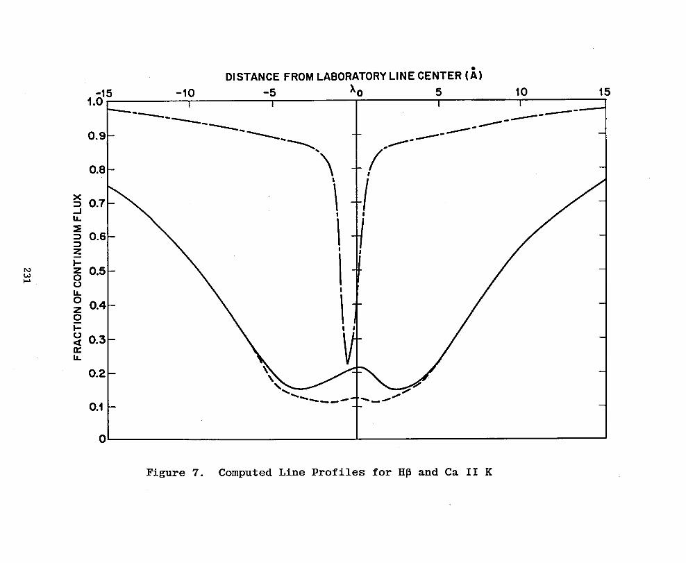
Figure 7 shows computed lines for the H8 and Ca II K

lines. The noticeable feature of the H8 line is thedepression of the continuum over a broad region of the

spectrum. Balmer line blanketing is thus predicted by

the models and is apparently confirmed by the results

of Table 1. The Ca II K line is quite broad and shows

a weak red shifted emission core. This emission core

results from the slight temperature inversion in the

outermost region of the model (Fig. 3). The dashed

line shows the change in the K line profile when this

outer shell in the model is arbitrarily removed during

the line profile calculation. The blue shifted profile

with a red shifted core seems to be in agreement with

the observations of Jacobsen (1956).

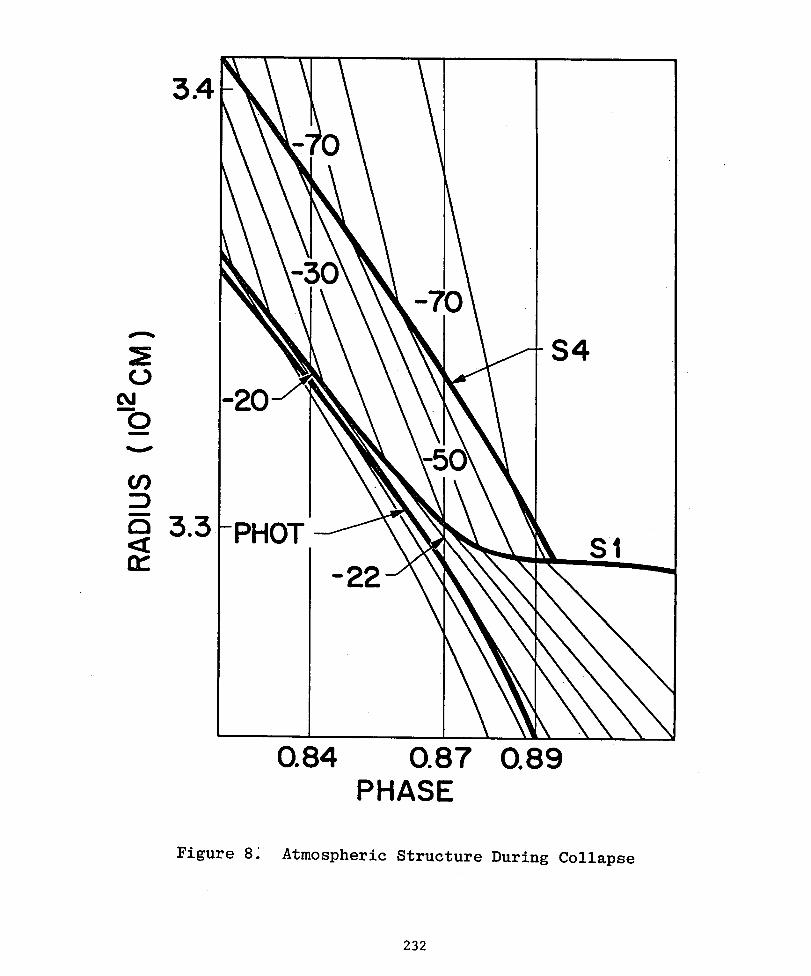
The SUPER NOVA model calculations also achieve some

success in predicting the complex behavior Which occurs

when the cepheid atmosphere collapses. Figure 8 shows

the predicted structure of the atmosphere for a 7.6 day

cepheid at several phases. The heavy lines indicate

various shock fronts and the photosphere. The finer

lines are radius-vs-time trajectories for various mass

220

zones in the model. The numerical values indicate the

local particle velocities in various regions.

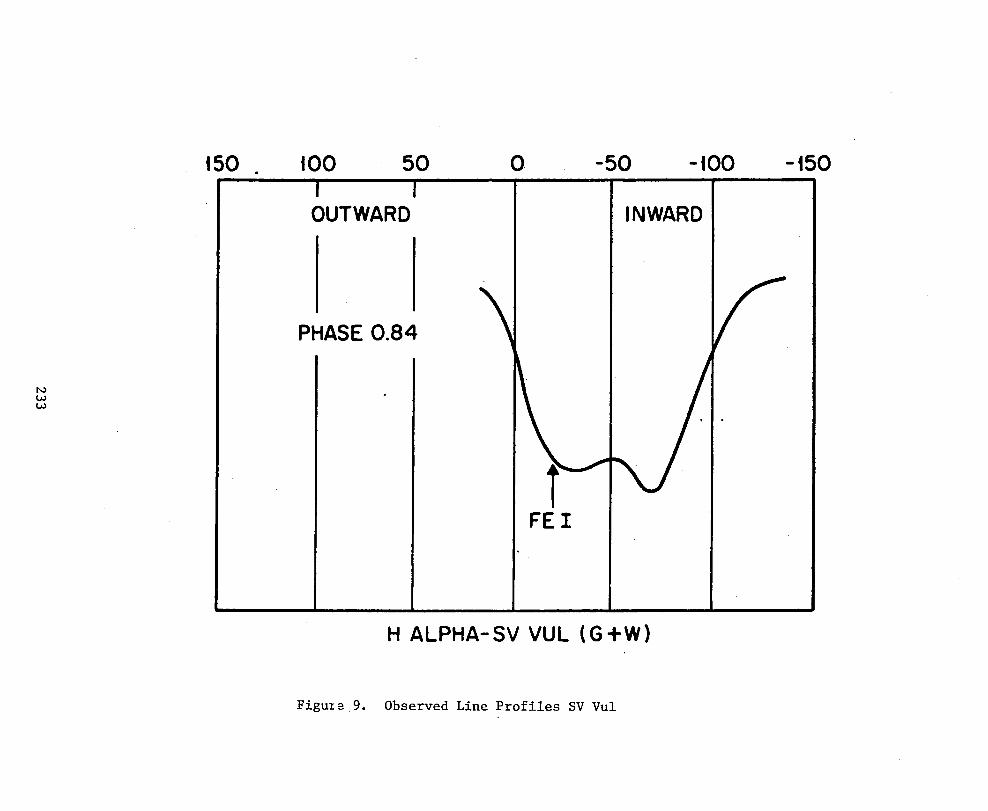
s

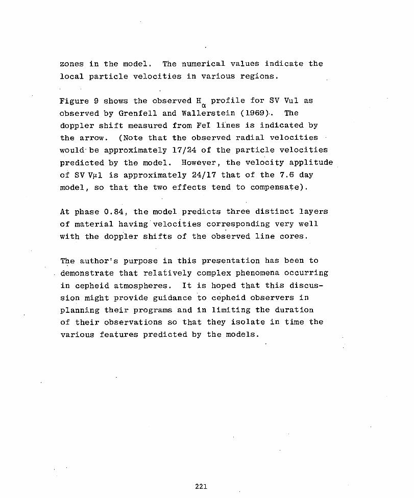
Figure 9 shows the observed H profile for SV Vul asaobserved by Grenfell and Wallerstein (1969). The

doppler shift measured from FeI lfnes is indicated by

the arrow. (Note that the observed radial velocities

would' be approximately 17/24 of the particle velocities

predicted by the model. However, the velocity applitude

of SV V_I is approximately 24/17 that of the 7.6 day

model, so that the two effects tend to compensate).

At phase 0.84, the model predicts three distinct layers

of material having velocities corresponding very well

with the doppler shifts of the observed line cores.

The author's purpose in this presentation has been to

demonstrate that relatively complex phenomena occurring

in cepheid atmospheres. It is hoped that this discus-

sion might provide guidance to cepheid observers in

planning their programs and in limiting the duration

of their observations so that they isolate in time the

various features predicted by the models.

221

REFERENCES

Brode, H. L. 1955, J. Appl. Phys. 26, 766.

Brode, H. L. 1956, RM-1824-AEC.

Brode, H. L. 1957, RM-1825-AEC.

Brode, H. L. 1958, RM-2247.

Brode, H. L. 1959a, RM-2248.

Brode, H. L. 1959b, RM-2249.

Brode, H. L. ed., 1965, "Reliability of Current NuclearBlast Calculations", Proceeding, of the DASAConference on Nuclear Weapons Effects and Re-EntryVehicles, DASA Report 1651 (Classified)

Christy, R. F. 1964, "Rev. Mod. Phys. 36," 555.

Christy, R. F. 1967, "Computational Methods in StellarPulsation", in Vol. 7 of "Methods in ComputationalPhysics" ed. B. Alder. Academic Press, New York.

Christy, R. F. 1968, Private Communication.

Grenfell, T. C., and Wallerstein, G. 1969, P.A.S.P. 8_!1,732.

Henyey, L. G., LeLevier, R., Levee, R. D., B6hm, K. H.,and Wilets, L. 1959, Astrophys. J. 129, 628.

Hillendahl, R. W. 1959, "Characteristics of the ThermalRadiation from Nuclear Detonations" AFSWP 902,Vols. I, II, III.

Hillendahl, R. W. 1962, Appendix B of "The SpectralAbsorption Coefficient of Heated Air", DASA 1348,Unclassified.

Hillendahl, R. W. 1964, "Approximation Techniques forRadiation - Hydrodynamics Calculations", DASA 1522,Unclassified.

Hillendahl, R. W. 1965a, Proceedings of the Workshop onthe Interdisciplinary Aspects of Radiative Transfer,J.I.L.A., ed. R. Goulard.

222

Hillendahl, R. W. 1965b, "Theoretical Models for NuclearFireballs" Part A, Lockheed Palo Alto ResearchLaboratories, DASA 1589 - LMSC BOO 6750, Unclassified.

Hillendahl, R. W. 1966, "Theoretical Models for NuclearFireballs (U)", DASA report 1589, Part B in 40volumes, (Classified).

Hillendahl, R._W. 1968, "Atmospheric Phenomena inClassical Cepheids", dissertation, University ofCalifornia at Berkeley.

Hillendahl, R. W. 1969, NBS Special Publication 332,"Spectrum Formation in Stars With Steady-StateExtended Atmospheres".

Hill'endahl, R. W. 1970, P.A.S.P. 82, 1231.

Jacobsen, T. S. 1956, Pub. Dom. Ap. Obs. Victoria, i0,145.

Oke, J. B. 1961, Ap.J. 133, 90.

Richtmyer, R. D., and Von Neumann, J. 1950, J. Appl.P_S. 21, 232.

Richtmyer, R. D. and Morton, K. W. 1967, "DifferenceMethods for Initial Valve Problems" Second Ed ,Interscience Publishers, New York.

Simpson. E. 1973, Science Applications, Inc., Palo Alto,California - Private Communication.

Schwarzschild, M., Schwarzschild, B., and Adams, W. S.1948, Ap.J. 108, 207.

Von Neumann, J., and Richtmyer, R. D. 1950, J. ApplPhys. 21, 232.

Whitney,C. 1955,Ap.J.121, 682.

223

224

3.9 ..........PhotosphericRadius

I

3.8

2.9-I I I I I I I _L, I I I I I

0.6 0.8 0 0.2 0.4 0.6 0.8:PHASE

Figure I. Radius-versus-phase for a Cepheid Model

225

Figure 2. Diagnostic Diagram for a Cepheid Model

226

10-7

i0 -8

EXPERIMENTAL LIGHT

.oo.o10_10

_ 54'

io-II.TEMPERATURE = 104_ h "I

10-123 × 1012 4 × 1012

RADIUS (cm) PHASE = 0.103

Figure 3o Atmospheric Profiles at Phase 0.103

227

10'8 I I I I I I I I I I I I I

J

S1 S1

$2 $3 @ ,$4

¢ejI

I°"_ •

ZN 0gl

0Ill

• SS&A LINES

O DYNAMIC MODEL

Figure 4. Density-versus-Phase for Eta Aquilae as Deducedfrom Two Types of Observations

i I I I I

4. • WESSELINK (WHITNEY)

O ABS. PHOTOMETRIC (WHITNEY)

• HEL. PHOTOMETRIC (OKE,MOD.) ..13REL. PHOTOMETRIC (PRESENT).

I0 0.5"

PHASE

FigureS. Radius-versus-Phase for Eta Aquilae

229

DISTANCEFROM LABORATORYLINE CENTER(A)-0.9 -0.8 -0.7 -0.6 -0.5 -0.4 -0.3 -0.2 -0.t 0 0.t 0.2

4.0 '" I \ _r----_ I _1 I I

k 1 \v:27 /Zo.8- _ _ \ //B 0.7- v:36/

_=_0'6- _2/ /F-Zo 0.5 I=0- r FIR)ohO

z 0.4-

_0.3u_

0.2-

0.| -

0

Figure 6. Computed Line Profiles for k4508_ Fe I

230

0

Figure 7. Computed Line Profiles for H_ and Ca II K

0.84 0.87 0.89PHASE

Figure 8: Atmospheric Structure During Collapse

232

t50 I00 50 0 -50 -I00 -150I IOUTWARD INWARD

PHASE0.84

L_L,O

FEI

;I

H ALPHA- SV VUL (G +W)

Figure 9. Observed Line Profiles SV Vul

Discussion

Adams: Do you have anythingto say about the mass anomally?

Hillendahl: I'm prejudiced. I used the low Christymass. I did a paper in

1955 that says the masses are about one half of what they shouldbe. This

techniqueI've talkedabout -- trying to use the maximumpossible observa-

tional datawith the'minimumpossible theoreticalinterpretation-- leads to

the same sort of result. What you are doing is taking lines that you hope

are in the photosphereand followingthem for a particularpart of the phase,

and if you integratethe velocityover that time, you get the absolutedis-

placementof that part of the cycle. If you differentiatethe velocity you

get g. The problem,isthen that you have absolutedisplacementover part of

the cycle but you don't have radius,so you have to go to some other technique

to get the relativeradius. If you do this, you end up with masses that are

too small comparedto the evolutionarymass.

Pe__!l:At the last Goddardconferencein'thisseries,Hutchinson,Hill and

Lilly presentedsome observationaldata for 8 Dor from the OAO-2 satellite.

They thoughtthey saw sharp blue peaks on the rising branch of this 10-day

Cepheid,which they interpretedas evidencefor shock waves. Togetherwith

J. Lub and J. Van ParadiJs,I observedthis star with the ANS satellite. I

think we have much better data and we do not see these blue peaks. On the

other hand, we have problems fittingthe whole rising branch of the light curve

with the Kurucz models. I don't find a satisfactoryequilibriummodel thato o

fits the energy distributionfrom 5500A to 1800A. So there is some evidence

for non-equilibriumradiation.

234

r

Hillendahl: Well, it's a questionof whetherit's non-equilibriumradiation

in the Dick Thomas sense or LTE radiationfrom a moving gas.

Pel: We can't distinguish between those two things. What we can say is that

there don'tseem to be pronounced short-llved peaks on the light curve there,

but the energy distribution cannot be represented well by a hydrostatic

equilibrium model atmosphere.

Hillendahl: No. In all deference to Stromgren, I think he was wrong. I

think Karl Schwarzschild was right. In 1905, his two-stream method was for

convective atmospheres, not for radiative ones. At the time I did this work,

the OAO-2 information on Cepheids was just beginning to come down. I think

they did see a little blip at 0.95, which is about where I would expect to

see the shock. One of the things you must be careful of in a model calculation

is the zoning. Simply because your code says there is a shock wave, it doesn't

necessarily mean you can see it. In a fireball model where your zoning is a

i meter scale, these effects are on a scale of" 0.i mm. There is a radiative

structure in which the gas dynamic discontinuity is embedded. There is a

paper by J. Zinn and R. C. Anderson (Phys. FI. 16, Nov. i0, 1973), in which

they have done the modeling of a radiative shock front. Shock fronts don't

always have that great brightness you might expect them to have. Only under

certain relationships between the density of the gas and the radiative mean

free path will you see the shock front itself. The rest of the time it's

going to be embedded in radiative precursors. So my guess is that your

ability to see shock waves is going to be very limited. Just a little bump

on the curve. Most of the gross features that you see that last for days and

235

days are caused by the progression of the photosphere inward due to hydro-

dynamlc expansion of the gases behind the front, and sometimes rarefaction

waves. I think you can show this quite easily.

J. Wood: In your fireball graph you mentioned a Christy reflection. What's

it reflecting off of?

Hillendahl: A fireball is quite different from a star. A star has a very

dense center. A fireball is essentially evacuated in the center, but none-

theless, the shock wave does reflect off the center. It makes a difference

(sort of a coefficient of restitution) what sort of materials and structure

you use. Particularly in the outer layers, it has been shownby comparison

with experiment that the equation of state is absolutely sacred.

236