Optical Flow Based Navigation

Samuel Kim and Vincent Kee

Department of Cognitive and Neural Systems, Boston University, Boston, MA

Department of Electrical and Computer Engineering, Boston University, Boston, MA

This paper deals with the viability of optic flow based navigation as implemented on a robot with a webcam. The first part discusses the need for such a technology, various filters that may be used to detect optic flow, and their effectiveness. The second part discusses the results and possible future directions of the project.

!

ABSTRACT:

As new technologies continue to develop, more and more robots are replacing humans in situations deemed too dangerous. However, current solutions are not fully automated, requiring offsite human operators for executing basic actions. The ideal solution would be a fully autonomous vehicle that could complete its objectives without any human intervention. In this project, the viability of optical flow based navigation was investigated. Optical flow, or optic flow, is the perception of object motion due to the object’s pixel shifts as the viewer moves relative to the environment. First, motion detection filters were developed and applied to image sequences in MATLAB. Then, they were implemented in optic flow based navigation MATLAB programs for an iRobot Create with a camera to provide video input. The robot successfully traversed through a textured environment but encountered difficulties when attempting to avoid textured obstacles and corners. Experiments were developed to compare the effectiveness of the Correlation and Gabor filters and to find the relationship between increased motion detection ability and processing time per frames. Possible future directions for this project include implementing GPU (Graphics Processing Unit), FPGA (Field-Programmable Gate Array), or even ASIC (Application-Specific Integrated Circuit) chips to speed up computation time, utilizing a wide-angle camera or an array of cameras to get a wider field of view, and integrating a q learning system.

INTRODUCTION:

In today's technological world, more and more autonomous machines are being designed to take the place of their human counterparts, especially in what are commonly known as dull, dangerous, and dirty

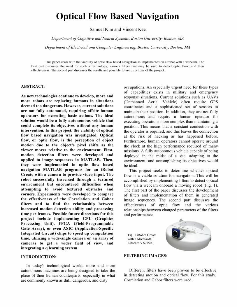
occupations. An especially urgent need for these types of capabilities exists in military and emergency response situations. Current solutions such as UAVs (Unmanned Aerial Vehicle) often require GPS coordinates and a sophisticated set of sensors to maintain their position. In addition, they are not fully autonomous and require a human operator for executing operations more complex than maintaining a position. This means that a constant connection with the operator is required, and this leaves the connection at the risk of hacking as has happened before. Furthermore, human operators cannot operate around the clock at the high performance required of many missions. A fully autonomous vehicle capable of being deployed in the midst of a site, adapting to the environment, and accomplishing its objectives would be ideal. This project seeks to determine whether optical flow is a viable solution for navigation. This will be accomplished by implementing filters to detect optical flow via a webcam onboard a moving robot (Fig. 1). The first part of the paper discusses the development of filters and implementation of them in generated image sequences. The second part discusses the effectiveness of optic flow and the various relationships between changed parameters of the filters and performance.

FILTERING IMAGES:

Different filters have been proven to be effective in detecting motion and optical flow. For this study, Correlation and Gabor filters were used.

Fig. 1 iRobot Create with a Microsoft Lifecam VX-5500!

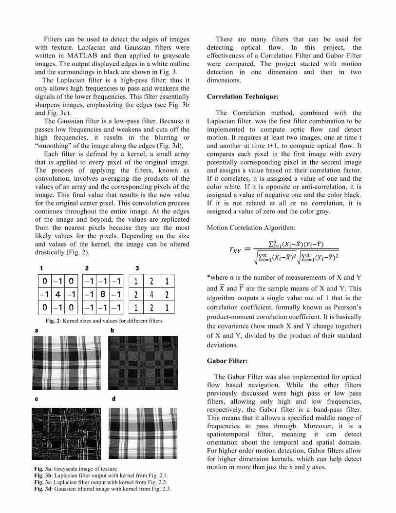
Fig. 3a: Grayscale image of texture Fig. 3b: Laplacian filter output with kernel from Fig. 2.1. Fig. 3c: Laplacian filter output with kernel from Fig. 2.2. Fig. 3d: Gaussian filtered image with kernel from Fig. 2.3.

Filters can be used to detect the edges of images with texture. Laplacian and Gaussian filters were written in MATLAB and then applied to grayscale images. The output displayed edges in a white outline and the surroundings in black are shown in Fig. 3. The Laplacian filter is a high-pass filter; thus it only allows high frequencies to pass and weakens the signals of the lower frequencies. This filter essentially sharpens images, emphasizing the edges (see Fig. 3b and Fig. 3c). The Gaussian filter is a low-pass filter. Because it passes low frequencies and weakens and cuts off the high frequencies, it results in the blurring or “smoothing” of the image along the edges (Fig. 3d). Each filter is defined by a kernel, a small array that is applied to every pixel of the original image. The process of applying the filters, known as convolution, involves averaging the products of the values of an array and the corresponding pixels of the image. This final value that results is the new value for the original center pixel. This convolution process continues throughout the entire image. At the edges of the image and beyond, the values are replicated from the nearest pixels because they are the most likely values for the pixels. Depending on the size and values of the kernel, the image can be altered drastically (Fig. 2).

1 2 3

a b

c d

There are many filters that can be used for detecting optical flow. In this project, the effectiveness of a Correlation Filter and Gabor Filter were compared. The project started with motion detection in one dimension and then in two dimensions. Correlation Technique: The Correlation method, combined with the Laplacian filter, was the first filter combination to be implemented to compute optic flow and detect motion. It requires at least two images, one at time t and another at time t+1, to compute optical flow. It compares each pixel in the first image with every potentially corresponding pixel in the second image and assigns a value based on their correlation factor. If it correlates, it is assigned a value of one and the color white. If it is opposite or anti-correlation, it is assigned a value of negative one and the color black. If it is not related at all or no correlation, it is assigned a value of zero and the color gray. Motion Correlation Algorithm:

!!" ! !!!!!!!!!!!!!!!!

!!!!!!!!!!! !!!!!!!!

!!!!

"where n is the number of measurements of X and Y and ! and ! are the sample means of X and Y. This algorithm outputs a single value out of 1 that is the correlation coefficient, formally known as Pearson’s product-moment correlation coefficient. It is basically the covariance (how much X and Y change together) of X and Y, divided by the product of their standard deviations.

Gabor Filter:

The Gabor Filter was also implemented for optical flow based navigation. While the other filters previously discussed were high pass or low pass filters, allowing only high and low frequencies, respectively, the Gabor filter is a band-pass filter. This means that it allows a specified middle range of frequencies to pass through. Moreover, it is a spatiotemporal filter, meaning it can detect orientation about the temporal and spatial domain. For higher order motion detection, Gabor filters allow for higher dimension kernels, which can help detect motion in more than just the x and y axes.

Fig. 2: Kernel sizes and values for different filters

Shifted Image

x (pixel)10 20

Dot

x (pixel)10 20

theta = 90 degreestheta = 45 degreestheta = 0 degreestheta = -45 degreestheta = -90 degrees

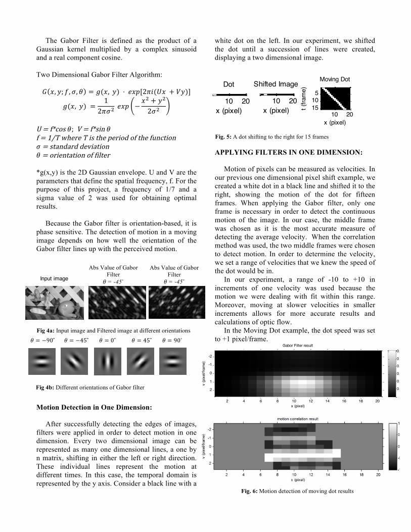
Fig 4a: Input image and Filtered image at different orientations

Gabor Filter result

x (pixel)

v (p

ixel

/fram

e)

2 4 6 8 10 12 14 16 18 20

-2

-1

0

1

2 0.05

0.1

0.15

0.2

0.25

0.3

Fig. 6: Motion detection of moving dot results

Input imageAbs Value of Gabor Filter

theta = -45 degrees

The Gabor Filter is defined as the product of a Gaussian kernel multiplied by a complex sinusoid and a real component cosine. Two Dimensional Gabor Filter Algorithm: ! !! !! !!!! ! ! !!!! !!!! ! !!"#!!!!!!"! ! !"!!!

!!!! !!!! ! !!!!! !!"# ! !

! ! !!!!! !

!"!#!$%&'(!!!!!)!#!$%(*+!!!$!#!,-.!/0121!.!*(!301!412*'5!'$!301!$6+&3*'+!!!#!(37+5725!518*73*'+!!!#!'2*1+373*'+!'$!$*9312!!*g(x,y) is the 2D Gaussian envelope. U and V are the parameters that define the spatial frequency, f. For the purpose of this project, a frequency of 1/7 and a sigma value of 2 was used for obtaining optimal results. Because the Gabor filter is orientation-based, it is phase sensitive. The detection of motion in a moving image depends on how well the orientation of the Gabor filter lines up with the perceived motion. !

Motion Detection in One Dimension:

After successfully detecting the edges of images, filters were applied in order to detect motion in one dimension. Every two dimensional image can be represented as many one dimensional lines, a one by n matrix, shifting in either the left or right direction. These individual lines represent the motion at different times. In this case, the temporal domain is represented by the y axis. Consider a black line with a

white dot on the left. In our experiment, we shifted the dot until a succession of lines were created, displaying a two dimensional image.

APPLYING FILTERS IN ONE DIMENSION:

Motion of pixels can be measured as velocities. In our previous one dimensional pixel shift example, we created a white dot in a black line and shifted it to the right, showing the motion of the dot for fifteen frames. When applying the Gabor filter, only one frame is necessary in order to detect the continuous motion of the image. In our case, the middle frame was chosen as it is the most accurate measure of detecting the average velocity. When the correlation method was used, the two middle frames were chosen to detect motion. In order to determine the velocity, we set a range of velocities that we knew the speed of the dot would be in. In our experiment, a range of -10 to +10 in increments of one velocity was used because the motion we were dealing with fit within this range. Moreover, moving at slower velocities in smaller increments allows for more accurate results and calculations of optic flow. In the Moving Dot example, the dot speed was set to +1 pixel/frame.

Moving Dot

x (pixel)

t (fra

me)

10 20

51015

Fig. 5: A dot shifting to the right for 15 frames

Abs Value of Gabor Filtertheta = 45 degrees

Abs Value of Gabor Filter ! = -45˚

Abs Value of Gabor Filter ! = -45˚

!!! ! !!"!!!!!!!!! ! !!"!!!!!!!!!! ! !"!!!!!!!!!!!!! ! !"#!!!!!!!!! ! !"˚

Fig 4b: Different orientations of Gabor filter

input

x (pixel)

y (p

ixel

)

10 20

10

20

shifted image

x (pixel)

y (p

ixel

)

10 20

10

20

X-T Plane

x (pixel)

t (fra

me)

5 10 15 20

2

4

6

8

10

12

14

16

18

20

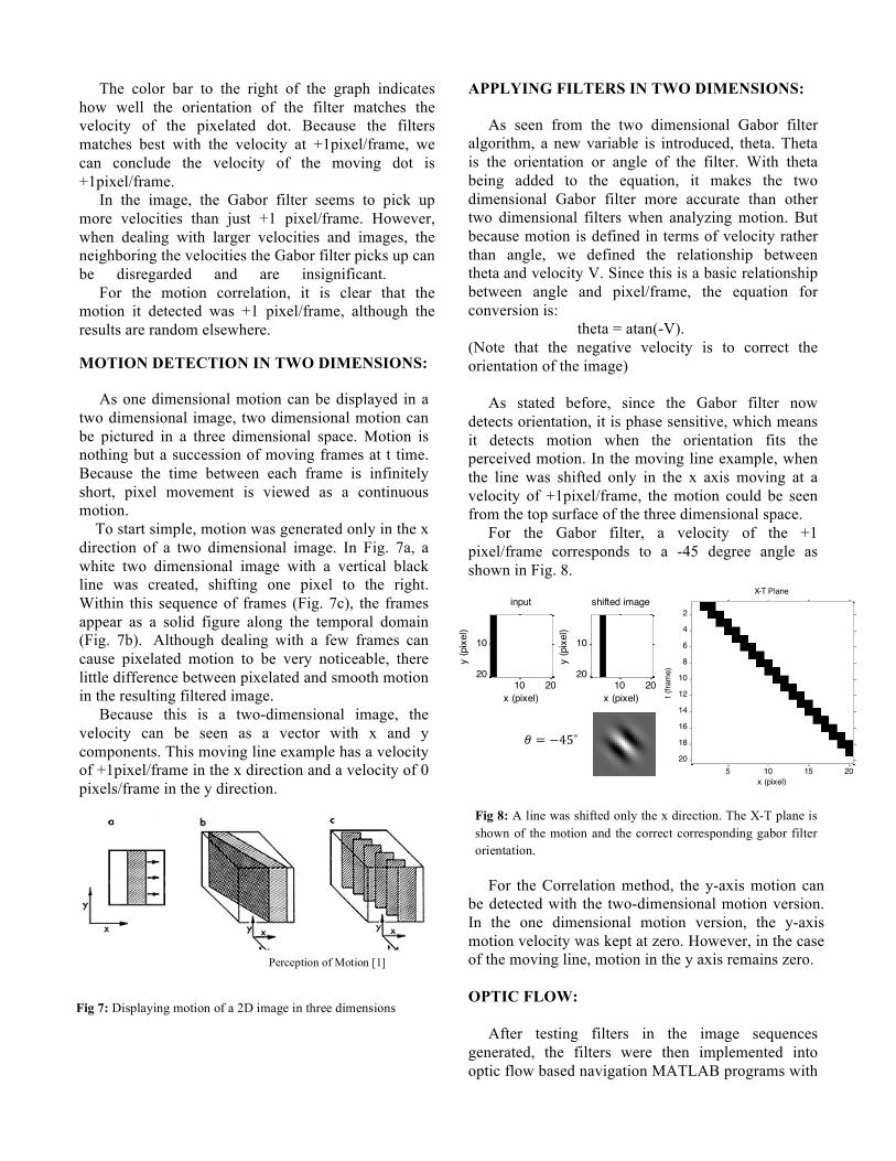
Fig 8: A line was shifted only the x direction. The X-T plane is shown of the motion and the correct corresponding gabor filter orientation.

theta = -45 degrees

The color bar to the right of the graph indicates how well the orientation of the filter matches the velocity of the pixelated dot. Because the filters matches best with the velocity at +1pixel/frame, we can conclude the velocity of the moving dot is +1pixel/frame. In the image, the Gabor filter seems to pick up more velocities than just +1 pixel/frame. However, when dealing with larger velocities and images, the neighboring the velocities the Gabor filter picks up can be disregarded and are insignificant. For the motion correlation, it is clear that the motion it detected was +1 pixel/frame, although the results are random elsewhere.

MOTION DETECTION IN TWO DIMENSIONS:

As one dimensional motion can be displayed in a two dimensional image, two dimensional motion can be pictured in a three dimensional space. Motion is nothing but a succession of moving frames at t time. Because the time between each frame is infinitely short, pixel movement is viewed as a continuous motion. To start simple, motion was generated only in the x direction of a two dimensional image. In Fig. 7a, a white two dimensional image with a vertical black line was created, shifting one pixel to the right. Within this sequence of frames (Fig. 7c), the frames appear as a solid figure along the temporal domain (Fig. 7b). Although dealing with a few frames can cause pixelated motion to be very noticeable, there little difference between pixelated and smooth motion in the resulting filtered image. Because this is a two-dimensional image, the velocity can be seen as a vector with x and y components. This moving line example has a velocity of +1pixel/frame in the x direction and a velocity of 0 pixels/frame in the y direction.

APPLYING FILTERS IN TWO DIMENSIONS:

As seen from the two dimensional Gabor filter algorithm, a new variable is introduced, theta. Theta is the orientation or angle of the filter. With theta being added to the equation, it makes the two dimensional Gabor filter more accurate than other two dimensional filters when analyzing motion. But because motion is defined in terms of velocity rather than angle, we defined the relationship between theta and velocity V. Since this is a basic relationship between angle and pixel/frame, the equation for conversion is:

theta = atan(-V). (Note that the negative velocity is to correct the orientation of the image) As stated before, since the Gabor filter now detects orientation, it is phase sensitive, which means it detects motion when the orientation fits the perceived motion. In the moving line example, when the line was shifted only in the x axis moving at a velocity of +1pixel/frame, the motion could be seen from the top surface of the three dimensional space. For the Gabor filter, a velocity of the +1 pixel/frame corresponds to a -45 degree angle as shown in Fig. 8. For the Correlation method, the y-axis motion can be detected with the two-dimensional motion version. In the one dimensional motion version, the y-axis motion velocity was kept at zero. However, in the case of the moving line, motion in the y axis remains zero. OPTIC FLOW: After testing filters in the image sequences generated, the filters were then implemented into optic flow based navigation MATLAB programs with

Perception of Motion [1]

Fig 7: Displaying motion of a 2D image in three dimensions

! ! !!"!!!!!

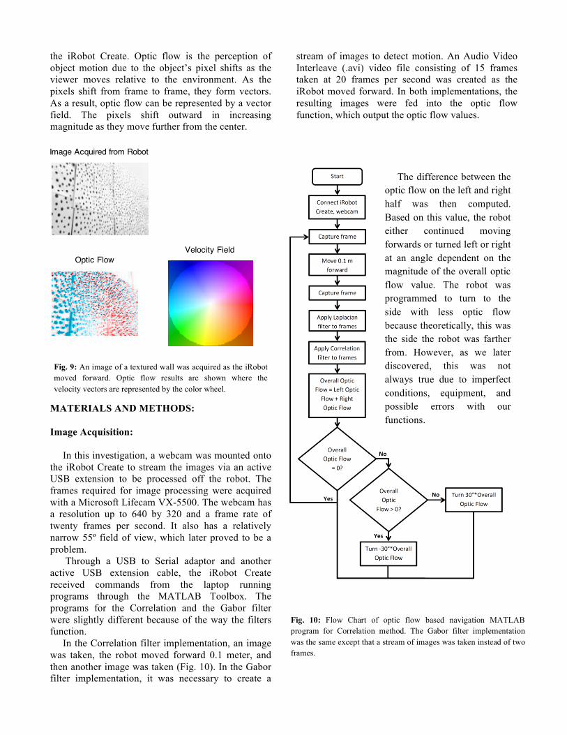
the iRobot Create. Optic flow is the perception of object motion due to the object’s pixel shifts as the viewer moves relative to the environment. As the pixels shift from frame to frame, they form vectors. As a result, optic flow can be represented by a vector field. The pixels shift outward in increasing magnitude as they move further from the center. MATERIALS AND METHODS: Image Acquisition: In this investigation, a webcam was mounted onto the iRobot Create to stream the images via an active USB extension to be processed off the robot. The frames required for image processing were acquired with a Microsoft Lifecam VX-5500. The webcam has a resolution up to 640 by 320 and a frame rate of twenty frames per second. It also has a relatively narrow 55º field of view, which later proved to be a problem. Through a USB to Serial adaptor and another active USB extension cable, the iRobot Create received commands from the laptop running programs through the MATLAB Toolbox. The programs for the Correlation and the Gabor filter were slightly different because of the way the filters function. In the Correlation filter implementation, an image was taken, the robot moved forward 0.1 meter, and then another image was taken (Fig. 10). In the Gabor filter implementation, it was necessary to create a

stream of images to detect motion. An Audio Video Interleave (.avi) video file consisting of 15 frames taken at 20 frames per second was created as the iRobot moved forward. In both implementations, the resulting images were fed into the optic flow function, which output the optic flow values.

Image Acquired from Robot

Optic FlowVelocity Field

Fig. 9: An image of a textured wall was acquired as the iRobot moved forward. Optic flow results are shown where the velocity vectors are represented by the color wheel.

The difference between the optic flow on the left and right half was then computed. Based on this value, the robot either continued moving forwards or turned left or right at an angle dependent on the magnitude of the overall optic flow value. The robot was programmed to turn to the side with less optic flow because theoretically, this was the side the robot was farther from. However, as we later discovered, this was not always true due to imperfect conditions, equipment, and possible errors with our functions.

!

Fig. 10: Flow Chart of optic flow based navigation MATLAB program for Correlation method. The Gabor filter implementation was the same except that a stream of images was taken instead of two frames.!

Program Parameters: We predicted that the increase in motion detection range directly correlates with an increase in processing times. To get the fastest performance, the range of velocities to detect for were set to be relatively small (11 pixels) and the robot was to move in small increments (0.1 meters) each time it stopped to take a frame. This way, the robot would start and stop in many small and relatively fast increments. In addition to this, we did not detect for vertical pixel shifts because we found that pixels did not move as noticeably in the y axis. Only horizontal motion was observed. This was also to speed up the processing time. In addition to varying the range of detected velocities, parts of image center were cut out where there was not much optic flow in order to speed up processing times. Like the range of pixel shifts, we tested and found that it too was directly correlated to processing time. To speed up the program, 320 pixels from the center were removed. We believed cutting out the center pixels would not significantly affect optical flow because the pixels in that spread had low pixel shifts that didn’t amount to much. By doing this, the size of the image was cut in half, theoretically doubling the speed of processing between each set of frames. TESTING:

Although we assumed the relationships between various factors of our factors and processing time, we created tests to determine the exact correlations between different parameters and processing time. Both filters require a predefined range of pixel shifts or velocities to detect for. The larger the range, the more velocities can be detected. Because time is a huge factor in real time navigation, time was measured based on different parameters in the filters in order to identify their relationships. The following tests were conducted:

- Range of Velocities versus Time - Size of Image Center versus Time - Resolution Size versus Time - Gabor Filter Size versus Time - Navigating an arena without bumping into

walls

Besides measuring Range of Velocities vs. Time, we measured the time based on how much of the

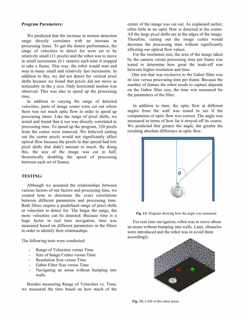
center of the image was cut out. As explained earlier, often little to no optic flow is detected at the center. All the large pixel shifts are at the edges of the image. Therefore, cutting out the image center would decrease the processing time without significantly affecting our optical flow values. For the resolution size, the area of the image taken by the camera versus processing time per frame was tested to determine how great the trade-off was between higher resolution and time. One test that was exclusive to the Gabor filter was its size versus processing time per frame. Because the number of frames the robot needs to capture depends on the Gabor filter size, the time was measured for the parameters of the filter. In addition to time, the optic flow at different angles from the wall was tested to see if the computation of optic flow was correct. The angle was measured in terms of how far it strayed off its course. We predicted that greater the angle, the greater the resulting absolute difference in optic flow. For real time navigation, robot was to move about an arena without bumping into walls. Later, obstacles were introduced and the robot was to avoid them accordingly.

!

Fig. 11: Diagram showing how the angle was measured!

Fig. 12: CAD of the robot arena

RESULTS:

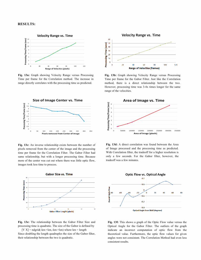
Fig. 13a: Graph showing Velocity Range versus Processing Time per frame for the Correlation method. The increase in range directly correlates with the processing time as predicted.!

Fig. 13b: Graph showing Velocity Range versus Processing Time per frame for the Gabor Filter. Just like the Correlation method, there is a direct relationship between the two. However, processing time was 3-4x times longer for the same range of the velocities. !

Fig. 13c: An inverse relationship exists between the number of pixels removed from the center of the image and the processing time per frame for the Correlation Filter. The Gabor Filter had same relationship, but with a longer processing time. Because more of the center was cut out where there was little optic flow, images took less time to process.!

Fig. 13d: A direct correlation was found between the Area of Image processed and the processing time as predicted. With Correlation filter, the tradeoff for a higher resolution is only a few seconds. For the Gabor filter, however, the tradeoff was a few minutes.!

Fig. 13e: The relationship between the Gabor Filter Size and processing time is quadratic. The size of the Gabor is defined by [Y X] = ndgrid(-len:+len,-len:+len) where len = length Since doubling the length quadruples the size of the Gabor filter, their relationship between the two is quadratic. !!!

Fig. 13f: This shows a graph of the Optic Flow value versus the Optical Angle for the Gabor Filter. The outliers of the graph indicate an incorrect computation of optic flow from the theoretical value. Furthermore, the optic flow values for given angles were not consistent. The Correlation Method had even less consistent results.!

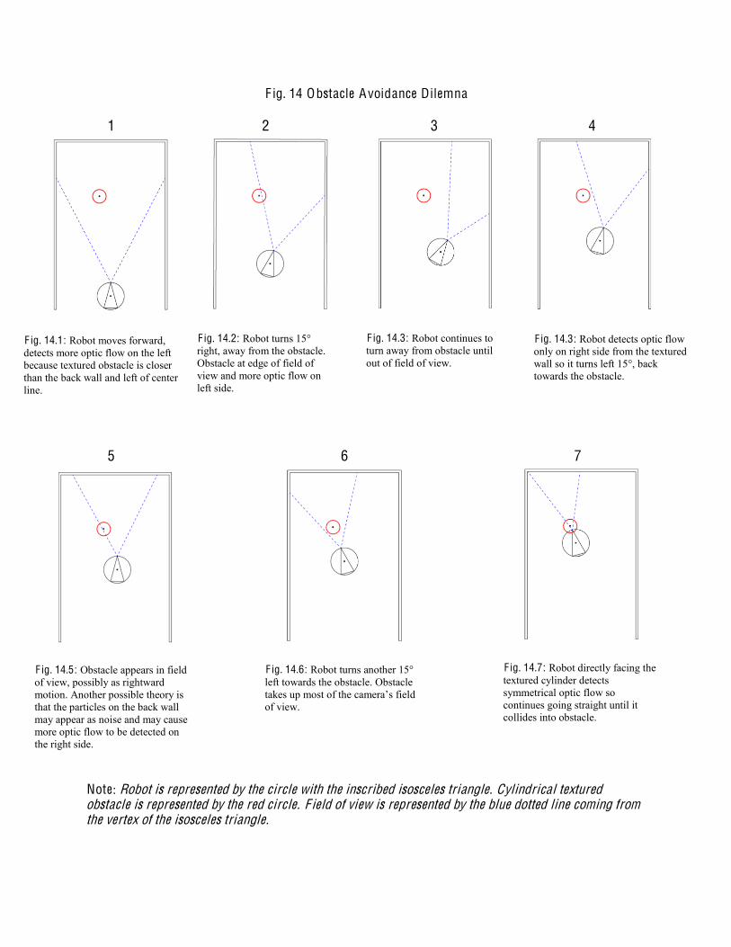
F ig. 14 Obstacle Avoidance Dilemna 1 2 3 4 5 6 7 Note: Robot is represented by the circle with the inscribed isosceles triangle. Cylindrical textured obstacle is represented by the red circle. F ield of view is represented by the blue dotted line coming from the vertex of the isosceles triangle.

F ig. 14.1: Robot moves forward, detects more optic flow on the left because textured obstacle is closer than the back wall and left of center line.

F ig. 14.2: Robot turns 15° right, away from the obstacle. Obstacle at edge of field of view and more optic flow on left side.

F ig. 14.3: Robot continues to turn away from obstacle until out of field of view.

F ig. 14.3: Robot detects optic flow only on right side from the textured wall so it turns left 15°, back towards the obstacle.

F ig. 14.5: Obstacle appears in field of view, possibly as rightward motion. Another possible theory is that the particles on the back wall may appear as noise and may cause more optic flow to be detected on the right side.

F ig. 14.6: Robot turns another 15° left towards the obstacle. Obstacle

of view.

F ig. 14.7: Robot directly facing the textured cylinder detects symmetrical optic flow so continues going straight until it collides into obstacle.

GABOR FILTER VS. CORRELATION:

The main difference between the Gabor filter and the Correlation method was the quality of the output of the optic flow field. For the Gabor filter, the velocity vectors were clearly seen in the flow field, but at the expense of significantly longer processing time. When using the Correlation technique, the direction of flow was in some cases hard to distinguish, but processing time was much quicker. However, in terms of navigation, the results were similar. Both methods could not replicate a successful navigation through the arena multiple times. Because many other factors were changing and had to be considered when computing the overall optic flow, each trial could not be replicated in the same way. CONCLUSION: Although our implementation of the optic flow based navigation program did successful traverse through a textured environment, many aspects of the application must change for optic flow to become a feasible method of navigation. First and foremost, the processing time per frame must be exponentially cut down. The processing time of the relatively faster Correlation method was anywhere from two to over ten seconds depending on the parameters. For real-time navigation, where a typical camera captures frames at 30 frames per second or higher, those frames must be all processed as the robot is moving and constantly receiving new frames. In addition, the two seconds achieved were with detecting pixel shifts from -10 to +10. For real world application, where drones such as the MQ-9 Reaper may be flying at up to 300 mph, the pixel shifts being detected must be much larger. The conclusion that the processing speed must be exponentially increased is perhaps an understatement. The next largest issue is the narrow field of view of the camera (55!!. This problem often led to incorrect computation of optic flow, sometimes even in the wrong direction, which all compounded into poor obstacle, wall, and corner avoidance. With a narrow field of view, the obstacle does not enter the view unless the iRobot is almost directly facing it. Once the robot is partway past the obstacle, it loses track of where the obstacle is until it reenters the field of view. At that point, as depicted in the Fig. 14.6, the obstacle fills the field of view and causes the robot to continue moving forward until it collides into the obstacle. In addition, there were problems when the iRobot encountered walls and corners face on. If the

iRobot moves towards walls and corners symmetrically, it computed equal but opposite values of optic flow from the left and right side, which resulted in little to no overall flow. Depending on the distance from the wall, this would not be considered a problem if the distance was far. However, when dealing with close proximities, the iRobot has trouble deciding whether to turn or go straight. If these two issues can be solved, the lofty goal of a fully autonomous and adaptable vehicle will be much closer to being accomplished. FUTURE DIRECTIONS:

There are many possible future directions for this project. First and foremost, the biggest issue is the slow image processing time. This is due in part to running the programs through MATLAB. Implementing the algorithms on a FPGA (Field-Programmable Gate Array) or even ASIC (Application-Specific Integrated Circuit) chip would significantly speed up the computations. Another possible solution would be to write code that would take advantage of GPUs with their parallel processing to do the optic flow computations.

To solve the issues with the narrow field of view, a wide angle webcam could be used. Another possible solution would be to use an array of webcams and then stitch the frames together to form one high quality panoramic image. This would allow the robot to keep obstacles in the field of view and allow the robot to avoid them more proficiently. The same would apply for wall navigation. Perhaps the most intriguing future direction for this project is to develop a robot q learning system. It would be a points reward system to 'teach' the robot to navigate using optic flow. The robot should be able to eventually avoid obstacles after many trial runs. For example, if the robot is navigating under certain conditions and it runs into an obstacle, it would get a negative point. Whenever the robot makes the correct decision and avoids the collision, the robot gets a positive point. Eventually, after repeatedly committing the same error, it would learn to avoid the obstacle. Ultimately, the robot would learn to adapt on its own. This feature, if successfully developed, would definitely get us closer to having robots that could function and adapt to new situations without human operators.

ACKNOWLEDGEMENTS We would like to thank Schuyler Eldridge, Florian Raudies, and Dr. Ajay Joshi for helping us immensely with this project. We could not have gone as far as we did without the help of Florian Raudies with the filters and optic flow concepts. Even sacrificing some of his work time to help us, he was a main driving force in our project. We would like to thank Schuyler Eldridge for helping us troubleshoot some of the key interfacing and performance issues with the iRobot Create implementations. We would like to thank Dr. Ajay Joshi for being our mentor and supporting us every step of the way. Even though he was extremely busy, he would always meet up and arrange time to check up on our progress. REFERENCES

1. Adelson, E.H., Bergen, J.R. (1985). Spatiotemporal energy models for the perception of motion. Journal of the Optical Society of America. A2, 284-299.

2. Chang, C.C., Chao, H.C., Chen, W.M., Lo, C.H. (2010). Gabor Filter 3D Ultra-Sonography Diagnosis System with WLAN Transmission Consideration. Journal of Universal Computer Science. 16: 1327-1342.

3. Esposito, J.M., Barton O. (2008). MATLAB Toolbox for the iRobot Create. www.usna.edu/Users/weapsys/esposito/roomba.matlab/

4. Heeger, D.J. (1987). Model for the extraction of image flow. Journal of the Optical Society of America. A4, 1455-1471.

5. Moore, R.J.D. Bhatti, Asim (Ed.). (2011). A Bio-Inspired Stereo Vision System for Guidance of Autonomous Aircraft, Advances in Theory and Applications of Stereo Vision. InTech. 16:305-326.

6. Orban, G.A., Hans-Hellmut, N., editors. (1992) Artificial and Biological Vision Systems. Luxembourg: Springer-Verlag. 389 p.

7. Reichardt, W. (1987). Evaluation of optical motion information by movement detectors. Journal of Comparative Physiology A. 161:533-547.