optical analysis for laser heterodyne communication system · optical analysis for laser heterodyne...
TRANSCRIPT
OPTICAL ANALYSIS FORLASER HETERODYNE COMMUNICATION SYSTEM
T. A. Nussmeier
Hughes Research Laboratories
3O11 Malibu Canyon RoadMalibu, California 9O265
(NASA-CB-1525U5) OPTICAL ANALYSIS FOB LASEB N77-81205HETEECDYNE COMMUNICATION SYSTEM FinalTechnical Report, 27 Nov. 1972 - 26 Nov.1973 (Huqiies Eesearch Lais.) 180 F UnclasPO/32:__JtQ.2.5J__
March 1974
Final Technical Report
Contract NAS 5-21898
Prepared for
GODDARD SPACE FLIGHT CENTERGreen belt, Maryland 2O771
REPRODUCED BY
NATIONAL TECHNICALINFORMATION SERVICE
U.S. DEPARTMENT OF COMMERCE
https://ntrs.nasa.gov/search.jsp?R=19770079983 2018-08-26T07:52:47+00:00Z
1. Report No. 2. Government Accession No. 3. Recipient's Catalog No.
4. Title and Subtitle'OPTICAL ANALYSIS FOR LASER HETERODYNE COMMUNICA-TION SYSTEM
5. Report Date
March 19746. Performing Organization Code
7. Author(s)T.A. NussmeierS.H. Brewer
8. Performing Organization Report No.
10. Work Unit No.9. Performing Organization Name and Address
Hughes Research Laboratories3011 Malibu Canyon RoadMalibu, California 90265
11. Contract or Grant No.
NAS 5-21898
12. Sponsoring Agency Name and Address
13. Type of Report and Period Covered27 Nov. 1972 through 26 Nov.Final Technical Report 197314. Sponsoring Agency Code
15. Supplementary Notes
16. Abstract
A new computer program has been developed to predict the effects of optical aberrations ontransmitters and receivers used in heterodyne communication systems. Two independent opticaltrains for the received signal and the local oscillator are specified and evaluated. A value ofheterodyne signal power is evaluated and normalized with respect to an ideal value to provide aquantitative value for receiver degradation. Values of local oscillator illumination efficiency,optical transmission, detection efficiency and phase match efficiency are also evaluated toisolate the cause of any unexpected degradations. The program has been used for a toleranceanalysis of a selected system designed for space communications, and for evaluation of severalother systems. Results of these analyses are presented.
17. Key Words (Suggested by AuthorlsH
Heterodyne CommunicationsNumerical AnalysisOptical Abbreviations (X\>.e;\V\.u •£'<•Space Applications
18. Distribution Statement
19. Security Qassif. (of this report)
UNCLASSIFIED
20. Security Classif. (of this page)
UNCLASSIFIED
21. No. of Pages
177
22. Price1
' For sale by the National Technical Information Service. Springfield. Virginia 22151
NASA-C-168 (Rev. fi-711
TABLE OF CONTENTS
Section Page
I INTRODUCTION AND SUMMARY 1
1. 1 Introduction 1
1. 2 Comparison with Other Optical ComputerPrograms 2
1. 3 Recommended Additions for IncreasedVersatility 4
1. 4 Summary 6
II LACOMA USER'S MANUAL 7
2. 1 General Program Description 7
2. 2 Data Discussion 15
2.3 Setting up the Data Deck 20
2.4 Data Preparation Procedure 21
2. 5 Input Format 22
2.6 Input Parameters 27
2.7 Interpretation of Output Data 38
2. 8 Coordinate — Sign ConventionSummary 42
2.9 Sample Cases 43
III SAMPLE SYSTEM ANALYSIS 47
IV DETAILED PROGRAM DESCRIPTION 65
4. 1 First Order Parameters 65
4.2 Image Location 69
4.3 Ray Trace - OPD 70
4.4 Vignetting and Obscuration 96
4. 5 Reference Wavefront 97
Section Page
4.6 Tilt and Decentration 104
4.7 Pupil Computations 109
4.8 Amplitude Spread Function 112
4.9 Receiver Quality Criteria 114
4.10 Transmitter Quality Criteria 117
4.11 Error Analyses 118
APPENDICES — Sample Cases
LIST OF ILLUSTRATIONS
Fig. 2-1. Basic flow diagram 8
Fig. 2-2. Transmitter computational flow 9
Fig. 2-3. Receiver computational flow 12
Fig. 2-4. Facsimile input sheet 12
Fig. 2-5. Output quadrants for ASF, PSF, pupilfunction 41
Fig. 3-1. Reference system optical schematic 48
Fig. 3-2. OMSS optical schematic 50
Fig. 3-3. Input deck for OM subsystem 53
Fig. 3-4. Primary-secondary separation error 56
Fig. 3-5. Effects of detector position 57
Fig. 3-6. Effects of tilted primary 58
Fig. 3-7. Effects of primary offset 59
Fig. 3-8. Field of view variation 62
Fig. 3-9. Optical schematic for afocal evaluation 63
Fig. 3-10. Results on Galilean telescope 64
Fig. 4-1. General paraxial ray notation 67
Fig. 4-2. Coordinate system and ray parameters 71
Fig. 4-3. Conic eccentricity parameters 73
Fig. 4-4. Cylindrical surface dur to RH01 but with^ wO 79
Fig. 4-5. (a) Cylindrical surface due to RH01 only . . . . 80
Fig. 4-5. (b) Cylindrical surface due to RH02 only . . . . 81
Fig. 4-6. Sinusoidal (cosine) surface error 83
IV
Fig. 4-7. Sinusoidal surface error with point symmetryof error decentered with respect to optical
Fig.
Fig.
Fig.
Fig.
Fig.
Fig.
Fig.
Fig.
Fig.
Fig.
Fig.
Fig.
Fig.
Fig.
Fig.
Fig.
4-8.
4-9.
4-10.
4-11.
4-12.
4-13.
4-14.
4-15.
4-16.
4-17.
4-18.
4-19.
4-20.
4-21.
4-22.
4-23.
Sinusoidal surface error with large displacementof error
Sine function surface error
Combined sine and cosine surface error . . . .
Racetrack obscuration (U = UZERO)
Rectangular obscuration
Rectangular or near-rectangular obscurationoriented 90 away from Figure 4-12
Circular clear aperture and obscuration . . .
Rectangular clear aperture andobscuration
Annular obscuration
Sample aperture configurations
Illustration of AY negative
Illustration of 0 positive
Uniform square ray grid
Deviations from the gaussian sphere
Description of circular aperture boundary byarray of square elements
Replicated (aliased) spread functions due todiscrete sampling of pupil
85
86
87
98
98
98
99
100
101
102
107
107
110
119
121
123
S E C T I O N I
INTRODUCTION AND SUMMARY
1.1 INTRODUCTION
The development of laser communication systems for space is
a vital step toward providing the nation with the capability for synchron-
ous relays, deep space probes, and ground stations. The special
properties of laser systems make such links possible without the need
for large antenna structures, and the need for high power as required
by microwave systems. Such a capability is particularly required,
within this decade, to furnish wideband data links from low altitude
satellites with high resolution sensors to earth synchronous communica-
tion terminals from which the information may then be relayed to
ground stations.
Spaceborne communication systems must necessarily operate
near theoretical thresholds. The demands against weight, prime
power, information rate, cost, reliability, and other factors do not
allow a large safety margin to compensate for overlooked degradations.
For this reason and others, the present computer program, LACOMA
(LAser COMmunicator Analysis program), has been developed to
accurately simulate optical configurations of heterodyne communication
systems and to evaluate the effects of aberrations, distortions and mis-
alignments on the heterodyne performance of these systems. The pro-
gram has been developed with the communication engineer in mind. It
has been designed to be easy to program and easy to interpret. Output
is specified in terms of antenna gain to allow results to be directly
applied to system calculations. Absolute power values are also printed
out to provide actual signal levels for evaluation.
1.2 COMPARISON WITH OTHER OPTICAL COMPUTER PROGRAMS
LACOMA represents a major advance in the optical analysis
of laser heterodyne communication systems. It also represents an
advance in general optical system analysis since it includes the effects
of gaussian pupil functions. Some of the optical analysis programs with
which LACOMA might be compared are:
1. POLYPAGOS —Aerospace Corporation
2. SLAP (Spectral Lens Analysis Program)— PAGOSCorporation
3. MTF— D. Grey Associates
4. ACCOS-GOALS— Scientific Computations Inc.
These represent a cross section of the generally available opti-
cal analysis programs and will serve as benchmarks to compare
LACOMA.
LACOMA is a direct descendant of SLAP which is in turn an
updated version of POLYPAGOS, so that one would logically expect
more similarities between these programs. An overview of the pro-
grams is provided by the tabular check sheet of Table I r l . A major
difference between these programs is the Fourier transform algorithms.
LACOMA (also SLAP and POLYPAGOS) utilizes an algorithm which per-
mits the specification of number and location of the output points for the
computed spread function (ASF, PSF) results. For a given optical
system or telescope, LACOMA allows sampling of the Airy disc via
grid sizes from 2x2 to 101x101 or any other arrays between these
extremes. This is not possible with the algorithms used by the other
programs. Not included in the table is a cost comparison. If it were
possible to set up a cost or running time comparison, the Gray-MTF
might show somewhat better due to its heavy emphasis on machine
language programming for the CDC 6600. The ACCOS-GOALS would
probably score as the most costly. Some of the tabulated categories
are subjective such as the ease of input, but they reflect more than a
single view.
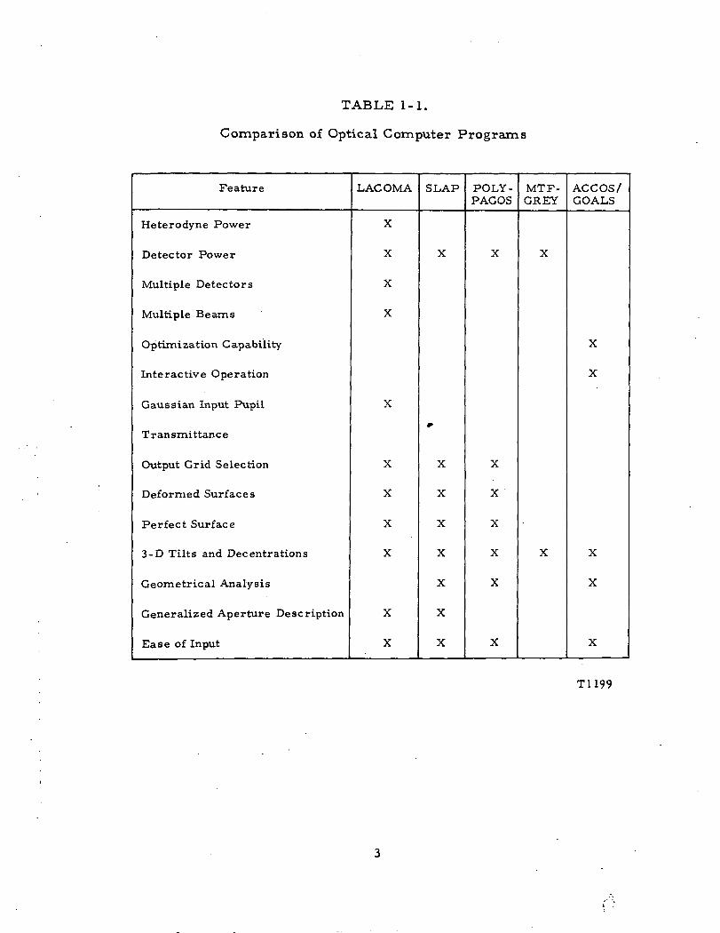
TABLE 1-1.
Comparison of Optical Computer Programs
Feature
Heterodyne Power
Detector Power
Multiple Detectors
Multiple Beams
Optimization Capability
Interactive Operation
Gaussian Input Pupil
Transmittance
Output Grid Selection
Deformed Surfaces
Perfect Surface
3-D Tilts and Decentrations
Geometrical Analysis
Generalized Aperture Description
Ease of Input
LACOMA
X
X
X
X
X
X
X
X
X
X
X
SLAP
X
r
X
X
X
X
X
X
X
POLY-PAGOS
X
X
X
X
X
X
X
MTF-GREY
X
X
ACCOS/GOALS
X
X
X
X
X
T1199

LACOMA constitutes a new tool in the optical communications
field. It is unique in its ability to perform an accurate analysis of the
laser communication system.
1.3 RECOMMENDED ADDITIONS FOR INCREASED VERSATILITY
LACOMA has been shown to be a unique and useful tool in the
analysis of heterodyne systems (see Section III). During the course of
using the program, it was often tempting to use it as a design tool.
This led to an investigation into the possibility of modifying the present
program to combine the features of design and analysis. The result
of this study led to the following list of recommended additions, some
of which would provide some design or optimization capability, and
others that would enhance the analysis function.
a. Optimization— Conventional optimization techniques will
not necessarily produce optimum optics for laser communication sys-
tems, especially for the transmitter and local oscillator. A gaussian
beam amounts to an aperture weighting function which should be included
in the optimization process. Also, ideally, the received signal optics
and local oscillator optics should be optimized on the basis of their
combined beams. It is recommended that work in the optimization
area occur in stages.
(1) Focus optimization— optimization of best focus posi-tion for a given system configuration.
(2) General optimization Phase I— Development ofalgorithms and approach to optimization for trans-mitter and receiver.
(3) General optimization— Phase II— Development ofoptimization program based on algorithms andapproach spelled out in Phase I.
b. Tolerance Analysis — Automatic determination of toler-
ance budgets necessary to maintain specified level of performance.
This can be a separately addressable subroutine of an optimization
program.
4
c. Perturbed Focal Surface— Revisions to permit tilted,
decentered, curved focal surface without dummy surfaces.
d. Return Option for Tilted-Dec entered Surfaces — To auto-
matically restore coordinate system after tilt and/or decentration
without dummy surfaces.
e. Aberrated Entrance Pupil — Accommodation of aberra-
tions of entrance pupil due to tilts-decentrations, input beam inclination.
f. Potato Chip Aspheres — Generalize deformed surface
options to include more generally deformed surfaces due to thermal-
mechanical stresses or potato chip aspheres.
g. Pseudo-diffraction Intensity Function — Geometrical
analysis to be used for evaluation of systems without involving full scale
diffraction-heterodyne analysis.
h. Transmittance — Subroutine to compute losses due to
absorption losses, Fresnel reflection losses, antireflection films,
multilayer thin films.Polarization — extension to determine orthogonal polarization
components of beam.
i. Graphics — Isometric and contour representation of wave
function, pupil function, spread functions, etc.
Interactive graphics — for analysis and optimization.
j. Fresnel Diffraction— Modification of diffraction integrals
of LACOMA to permit computation of amplitude or intensity function out
of Fraunhofer plane.
k. Thermal-mechanical Structural Analysis — Extension of
LACOMA to interface with thermal-mechanical analysis programs such
as STARDYNE, NASTRAN, etc., to perform overall system analysis.
Some of the listed modifications are contained in other programs
as seen in Table 2-1, while others, such as transmittance, are unique.
Transmittance in particular should be considered for LACOMA, since
this parameter affects the amplitude distribution across the exit pupil,
which, in turn, can make a significant difference in phase distribution
across the focal plane, and can also cause a shift in the location of the
5
focal plane. Other modifications that are considered particularly
appropriate to heterodyne systems are focus optimization, perturbed
focal surfaces, and the related Fresnel diffraction modification.
1.4 SUMMARY
Section II of this report is designed to be a self-contained user's
manual. An engineer familiar with heterodyne optical systems should
be able to utilize LACOMA with this manual and a minimal amount of
help from computer personnel..
Section III contains an analysis of the sample system, the opti-
cal mechanical subsystem developed for NASA under contract NAS-
5-21859. This analysis includes a "perfect" reference system, several
runs for the system with no distortions or errors, and finally analyses
with tilts and distortions that might be introduced by manufacturing
tolerances or by mechanical or thermal stress. This section has been
arranged to provide a specific example for using LACOMA.
At the end of Section III, two additional analyses are summarized,
one that establishes bounds on the field of view of heterodyne receivers,
and a second that analyzes a telescope designed for a terrestrial system.
This last example was selected because there is sufficient aberration to
cause significant performance degradation, thus providing a means for
illustrating the advantages of LACOMA over conventional optical
programs.
Section IV contains a detailed discussion of the program.
Specific equations and computational flow diagrams are discussed.
Error sources and their probable magnitudes are covered at the end
of this section.

S E C T I O N II
LACOMA USER'S MANUAL
2. 1 GENERAL PROGRAM DESCRIPTION
The program has been developed to allow prediction of laser
communication system performance and to permit tradeoff analysis in
the design of these systems. The program is set up to allow the
optional analysis of transmitter or receiver optics.
For the transmitter, the program starts with the data for the
specified laser beam and propagates the beam through the optical train
to determine the far-field intensity function.
For the receiver, the program carries the received signal beam
through the optical train to the detector. The local oscillator laser
beam is also traced to the detector where the two beams are combined
and the various quality criteria computed.
The computation for the receiver requires the entry of two sets
of optical data— one for the received signal optics and another for the
local oscillator optics. The program checks whether one or two sets
of data have been entered (see Fig. 2-1). If there is only one set, it
performs the transmitter analysis. Two sets of data precipitate the
receiver analysis.
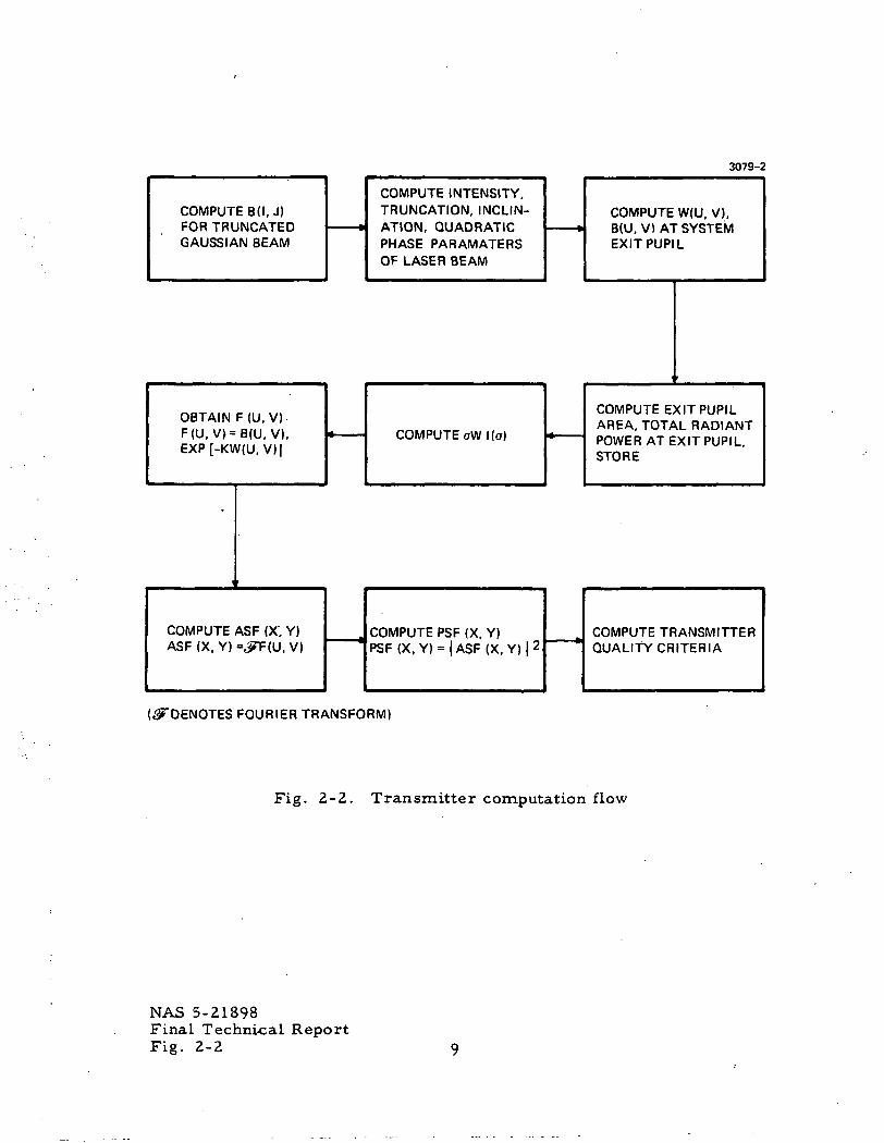
a. Transmitter— For a single set of optical data the pro-
gram computes the gaussian beam profile and any specified quadratic
phase on the input beam and traces it through the optical train, carrying
the complex amplitude function through in the form of an amplitude
array B (i, j), and the optical path difference array W (i, j) (see Fig. 2-2) .
At the exit pupil it computes the rms wavefront error crW and the
normalized Strehl intensity I (<r) for the (systematic) system wavefront.
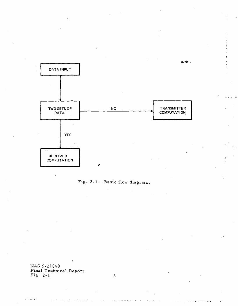
DATA INPUT
TWO SETS OFDATA
YES
RECEIVERCOMPUTATION
3079-1
NO TRANSMITTERCOMPUTATION
Fig. 2-1. Basic flow diagram.
NAS 5-21898Final Technical ReportFig. 2-1
3079-2
COMPUTE Bd, J)FOR TRUNCATEDGAUSSIAN BEAM
COMPUTE INTENSITY.TRUNCATION, INCLIN-ATION! ("11 IAPIR ATIPPHASE PAR AM ATE RSOF LASER BEAM
COMPUTE W(U, V),B(U, VI AT SYSTEMEXIT PUPIL
OBTAIN F(U, V)F(U V)~ B(U V)EXP[-KW(U, V)]
COMPUTE aWI (a)
COMPUTE EXIT PUPILAREA, TOTAL RADIANTPOWER AT EXIT PUPIL,STORE
COMPUTE ASF (X, Y)ASF (x, Y) =grt(\j. v)
COMPUTE PSF (X, Y)PSF(X,Y) = |ASF(X, Y ) | 2
COMPUTE TRANSMITTERQUALITY CRITERIA
(^DENOTES FOURIER TRANSFORM)
Fig. 2-2. Transmitter computation flow
NAS 5-21898Final Technical ReportFig. 2-2
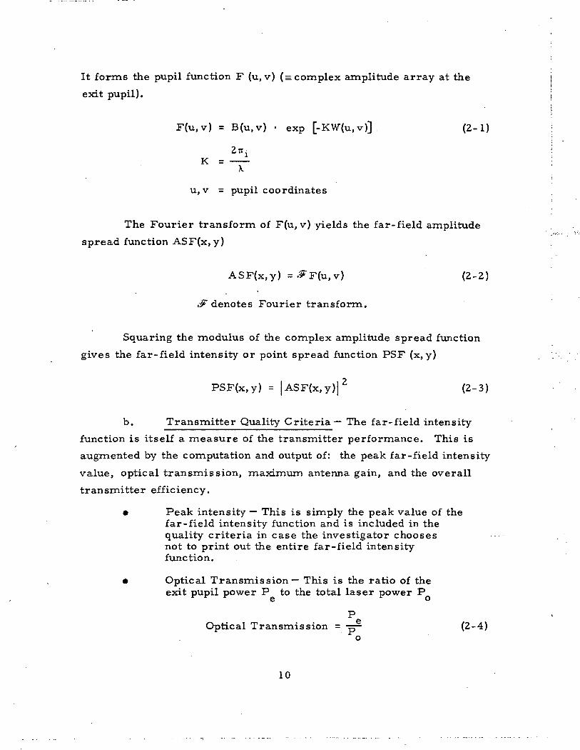
It forms the pupil function F (u,v) (= complex amplitude array at the
exit pupil).
F(u,v) = B(u,v) • exp [-KW(u.v)] (2-1)
2"i\£ — _____
X
u, v = pupil coordinates
The Fourier transform of F(u, v) yields the far-field amplitude
spread function ASF(x, y)
ASF(x,y) = ^"F(u,v) (2-2)
^denotes Fourier transform.
Squaring the modulus of the complex amplitude spread function
gives the far-field intensity or point spread function PSF (x, y)
PSF(x,y) = |ASF(x,y)|2 (2-3)
b. Transmitter Quality Criteria— The far-field intensity
function is itself a measure of the transmitter performance. This is
augmented by the computation and output of: the peak far-field intensity-
value, optical transmission, maximum antenna gain, and the overall
transmitter efficiency.
• Peak intensity — This is simply the peak value of thefar-field intensity function and is included in thequality criteria in case the investigator choosesnot to print out the entire far-field intensityfunction.
• Optical Transmission— This is the ratio of theexit pupil power P to the total laser power P
POptical Transmission = -p^ (2-4)
o
10
Transmission losses accounted for here are those dueto vignetting and obscuration.
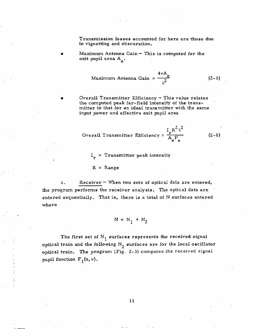
Maximum Antenna Gain — This is computed for theexit pupil area A .
4-nAMaximum Antenna Gain = r— (2-5)
Overall Transmitter Efficiency — This value relatesthe computed peak far-field intensity of the trans-mitter to that for an ideal transmitter with the sameinput power and effective exit pupil area
I rR2X2
Overall Transmitter Efficiency = . p— (2-6)e e
I = Transmitter peak intensity
R = Range
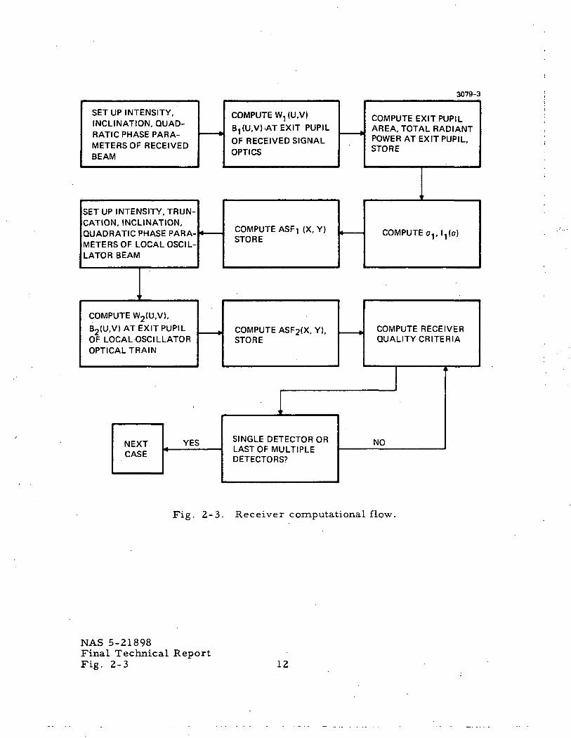
c. Receiver— When two sets of optical data are entered,
the program performs the receiver analysis. The optical data are
entered sequentially. That is, there is a total of N surfaces entered
where
N = Nj + N2
The first set of N, surfaces represents the received signal
optical train and the following N_ surfaces are for the local oscillator
optical train. The program (Fig. 2-3) computes the received signal
pupil function F,(u, v).
11
3079-3
SET UP INTENSHINCLINATION, QRATIC PHASE PAMETERS OF RECBEAM
"Y,JAD-RA-EIVED
SET UP INTENSITYCATION, INCLINATQUADRATIC PHASEMETERS OF LOCALLATOR BEAM
1
TRUN-ION,1 PARA-OSCIL-
COMPUTE W2(U,V),
B2(U,V) AT EXIT PUPILOF LOCAL OSCILLATOROPTICAL TRAIN
NEXTCASE
YES
COMPUTE W, (U,V)
B^U.VJiATEXIT PUPIL
OF RECEIVED SIGNALOPTICS
COMPUTE EXIT PUPILAREA, TOTAL RADIANTPOWER AT EX IT PUPIL,STORE
1 '
COMPUTE ASF \ (X, Y)STORE
COMPUTE av l^o)
COMPUTE ASF2(X, Y),STORE
COMPUTE RECEIVERQUALITY CRITERIA
1 '
SINGLE DETECTOR ORLAST OF MULTIPLEDETECTORS?
NO
Fig. 2-3. Receiver computational flow.
NAS 5-21898Final Technical ReportFig. 2-3 12
_ P DNonheterodyne Detection Efficiency = •=— (2-12)
L.O. illumination Efficiency_— This efficiency com-pares the heterodyne power P, for the two givensignals with no phase error wvth the optimumheterodyne power value for two signals of cor-responding power
PhL. O. Illumination Efficiency = — (2-13)
Maximum Antenna Gain— This is the theoreticalgain for the effective entrance pupil area A ofthe received signal optical train.
4irAMaximum Antenna Gain = —j- (2-14)
Receiver Efficiency to i.f. — Assuming a quantumefficiency of 1, this efficiency relates the squareof the heterodyne power P^ to the product of thetotal received power PQ and the L.O. power PL,and is a measure of overall receiver performance.
Receiver Efficiency to i.f. = p ^ (2-15)<> L
2. 2 DATA DISC USSION
The program performs analyses on laser communication system
optics as summarized in Section 2-1 with the detailed computational
procedure described in Section IV of this document. The analyses per-
formed by the program are briefly listed here.
Paraxial Analysis (Section 4. 1)
Ray Trace-Optical Path Difference (Section 4.3)
15
Amplitude and Point Spread Function (Section 4. 8)
Receiver Quality Criteria.(Section 4.9)
Transmitter Quality Criteria (Section 4. 10)
Numerous options are available for handling of the data, choice
of computations, output data, etc. Two data arrays IPRQ0G and IDETEC
control the major functions and are discussed in detail.
Some optical system parameters and/or configurations which
can be accommodated by LACOMA include:
• Catoptric systems
• Catadioptric systems
• Dioptric systems
• Spherical surfaces
• Aspheres
• Cylindrical surfaces
• Toroidal surfaces
• Surfaces with slight cylindrical error or warpage
• Periodic surface errors
• Misaligned (tilted, and/or decentered) systems
• Composite vignetting and obscuration
• Afocal systems (via perfect imaging lens)
Any of the analyses can be performed for any of the system
parameters or configurations.
a. Data Requirements — A certain minimum amount of data
must be entered to obtain any results. These minimum data require-
ments can combine with built-in data or default conditions to give a
complete system analysis. These data are listed here with their
associated program variable names and text references.
16
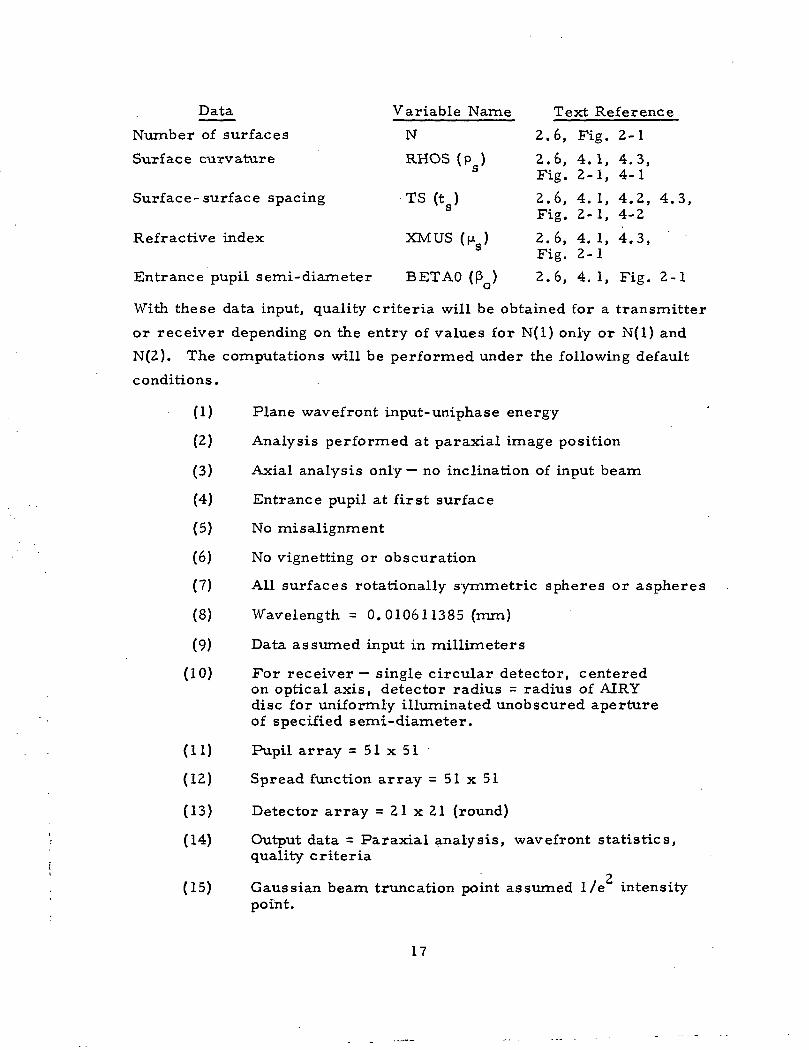
Data Variable Name Text Reference
Number of surfaces N 2.6, Fig. 2-1
Surface curvature RHOS (p ) 2.6, 4.1, 4.3,s Fig. 2-1, 4-1
Surf ace-surf ace spacing TS (t ) 2.6, 4.1, 4.2, 4.3,3 Fig. 2-1, 4-2
Refractive index XMUS (PL ) 2.6, 4.1, 4.3,8 Fig. 2-1
Entrance pupil semi-diameter BETAO (p ) 2.6, 4.1, Fig. 2-1
With these data input, quality criteria will be obtained for a transmitter
or receiver depending on the entry of values for N(l) only or N(l) and
N(2). The computations will be performed under the following default
conditions.
(1) Plane wavefront input-Uniphase energy
(2) Analysis performed at paraxial image position
(3) Axial analysis only— no inclination of input beam
(4) Entrance pupil at first surface
(5) No misalignment
(6) No vignetting or obscuration
(7) All surfaces rotational!/ symmetric spheres or aspheres
(8) Wavelength = 0. 010611385 (mm)
(9) Data assumed input in millimeters
(10) For receiver— single circular detector, centeredon optical axis, detector radius = radius of AIRYdisc for uniformly illuminated unobscured apertureof specified semi-diameter.
(11) Pupil array = 51 x 51
(12) Spread function array = 5 1 x 5 1
(13) Detector array = 21 x 21 (round)
(14) Output data = Paraxial analysis, wavefront statistics,quality criteria
(15) Gaussian beam truncation point assumed 1/e intensitypoint.
17
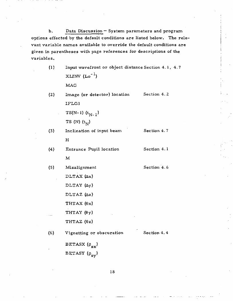
b. Data Discussion— System parameters and program
options effected by the default conditions are listed below. The rele-
vant variable names available to override the default conditions are
given in parentheses with page references for descriptions of the
variables.
(1) Input wavefront or object distance Section 4. 1, 4.7
XLJNV (Lo"1)
MAG
(2) Image (or detector) location Section 4. 2
IFLG1
TS(N-l) ( t N _ x )
TS (N) (tN)
(3) Inclination of input beam Section 4.7
H
(4) Entrance Pupil location Section 4. 1
M
(5) Misalignment Section 4. 6
DLTAX (Ax)
DLTAY (Ay)
DLTAZ (Az)
THTAX (6x)
THTAY (6y)
THTAZ (6z)
(6) Vignetting or obscuration Section 4.4
BETASX (6 )vrsx
BETASY (p )
18
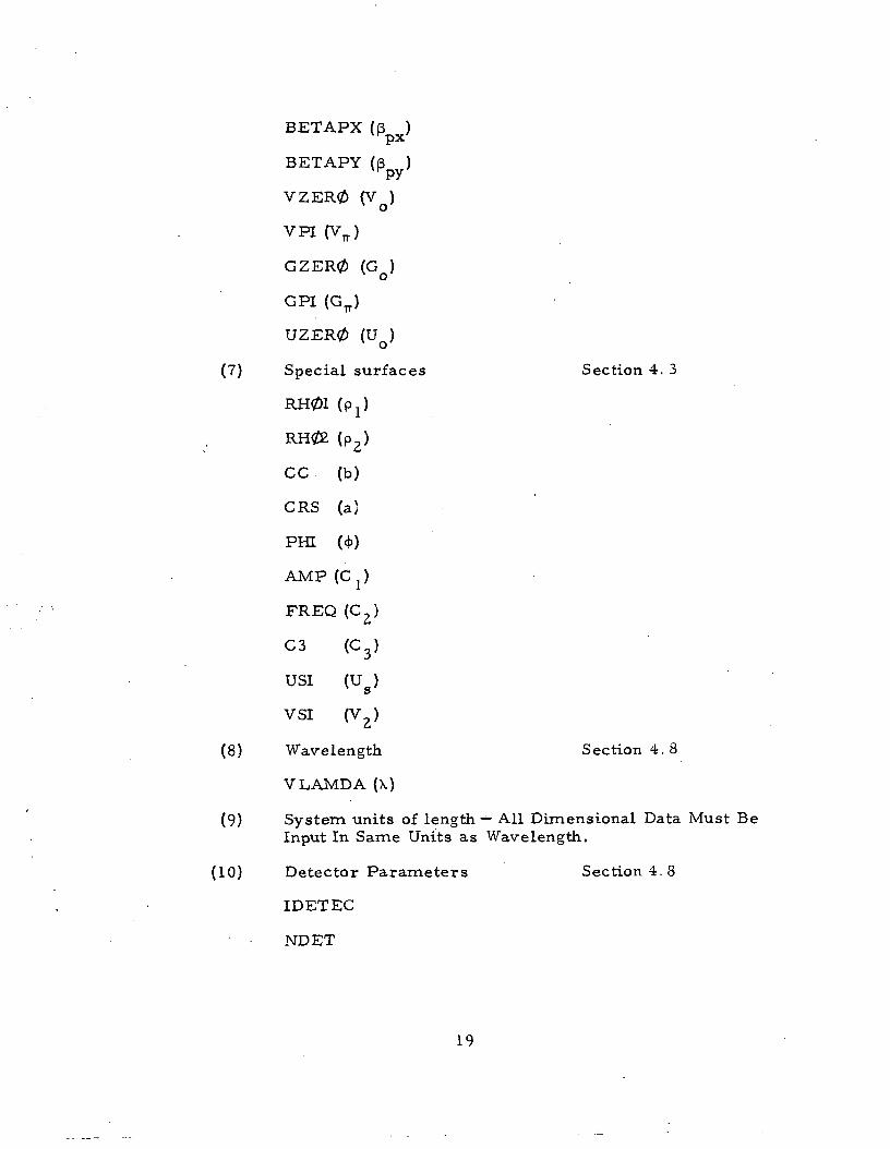
(7)
(8)
(9)
(10)
BETAPX (p )
BETAPY (p )
VZER0 (V )
VPI (VJ
GZER0 (GQ)
GPI (GJ
UZER0 (U )
Special surfaces
RH01 ( P )
(p2)
CC (b)
CRS (a)
PHI (4>)
AMP (C )
<c3)
'Us>
FREQ (C2)
C3
USI
vsi (V2)
Wavelength
VLAMDA (\)
Section 4. 3
Section 4. 8
System units of length — All Dimensional Data Must BeInput In Same Units as Wavelength.
Detector Parameters
IDETEC
NDET
Section 4. 8
19
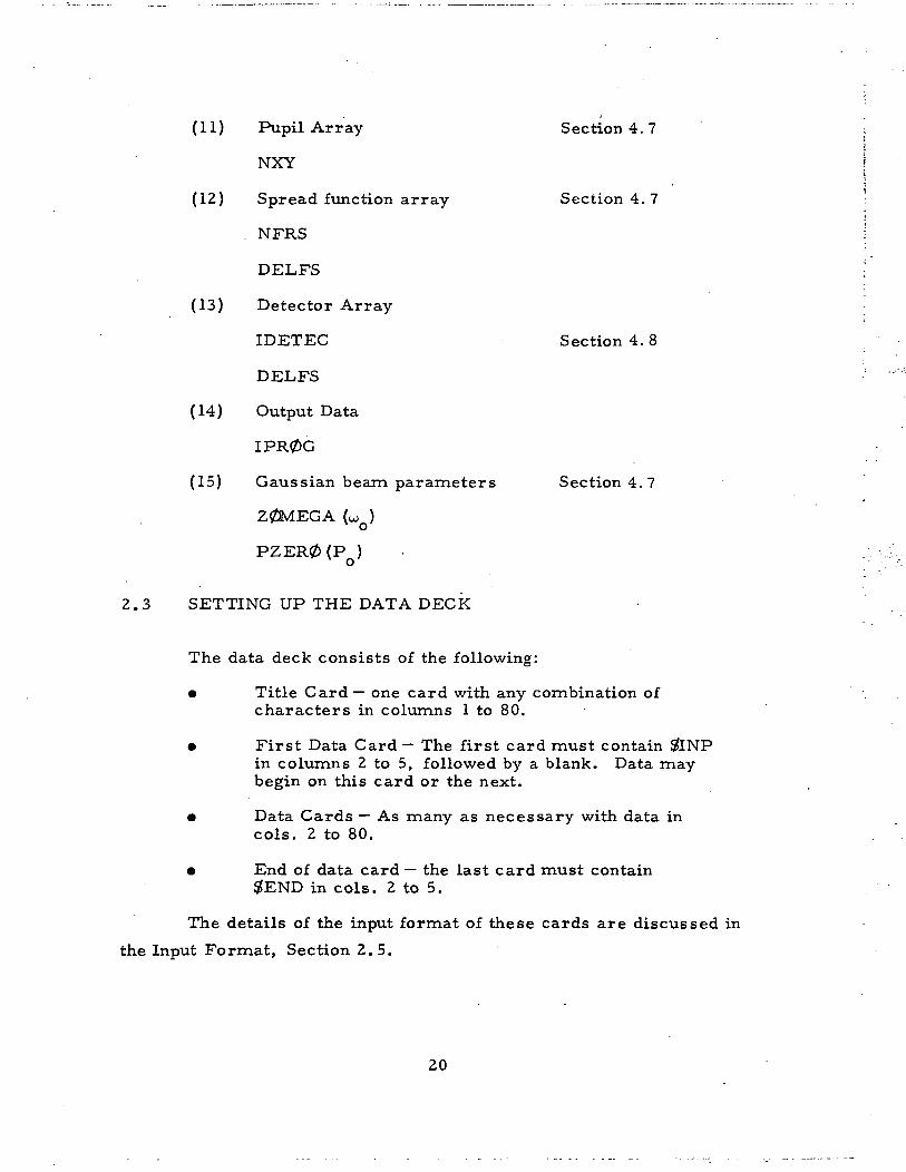
(11) Pupil Array Section 4.7
NXY
(12) Spread function array Section 4.7
. NFRS
DELFS
(13) Detector Array
IDETEC Section 4. 8
DELFS
(14) Output Data
IPR0G
(15) Gaussian beam parameters Section 4.7
Z0MEGA (w )
PZER0(P )
2.3 SETTING UP THE DATA DECK
The data deck consists of the following:
• Title Card— one card with any combination ofcharacters in columns 1 to 80.
• First Data Card— The first card must contain SftNPin columns 2 to 5, followed by a blank. Data maybegin on this card or the next.
• Data Cards — As many as necessary with data incols. 2 to 80.
• End of data card — the last card must contain#END in cols. 2 to 5.
The details of the input format of these cards are discussed in
the Input Format, Section 2.5.
20
The details of the individual data are given in Input Parameters,
Section 2.6.
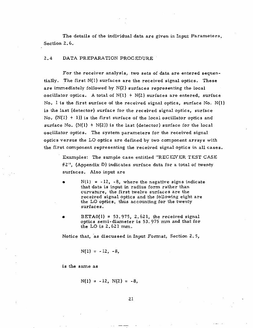
2.4 DATA PREPARATION PROCEDURE
For the receiver analysis, two sets of data are entered sequen-
tially. The first N(l ) surfaces are the received signal optics. These
are immediately followed by N(2) surfaces representing the local
oscillator optics. A total of N(l) -f N(2) surfaces are entered, surface
No. 1 is the first surface of the received signal optics, surface No. N(l)
is the last (detector) surface for the received signal optics, surface
No. (N(l) + 1)) is the first surface of the local oscillator optics and
surface No. (N(l) + N(2)) is the last (detector) surface for the local
oscillator optics. The system parameters for the received signal
optics versus the LO optics are defined by two component arrays with
the first component representing the received signal optics in all cases.
Examples: The sample case entitled "RECEIVER TEST CASE
#2", (Appendix D) indicates surface data for a total of twenty
surfaces. Also input are
• N ( l ) = -12, -8, where the negative signs indicatethat data is input in radius form rather thancurvature, the first twelve surfaces are thereceived signal optics and the following eight arethe LO optics, thus accounting for the twentysurfaces.
• BETAO(l) = 53.975, 2.621, the received signaloptics semi-diameter is 53. 975 mm and that forthe LO is 2.621 mm.
Notice that, as discussed in Input Format, Section 2. 5,
N(l) = -12, -8,
is the same as
N(l) = -12, N(2) = -8,
21
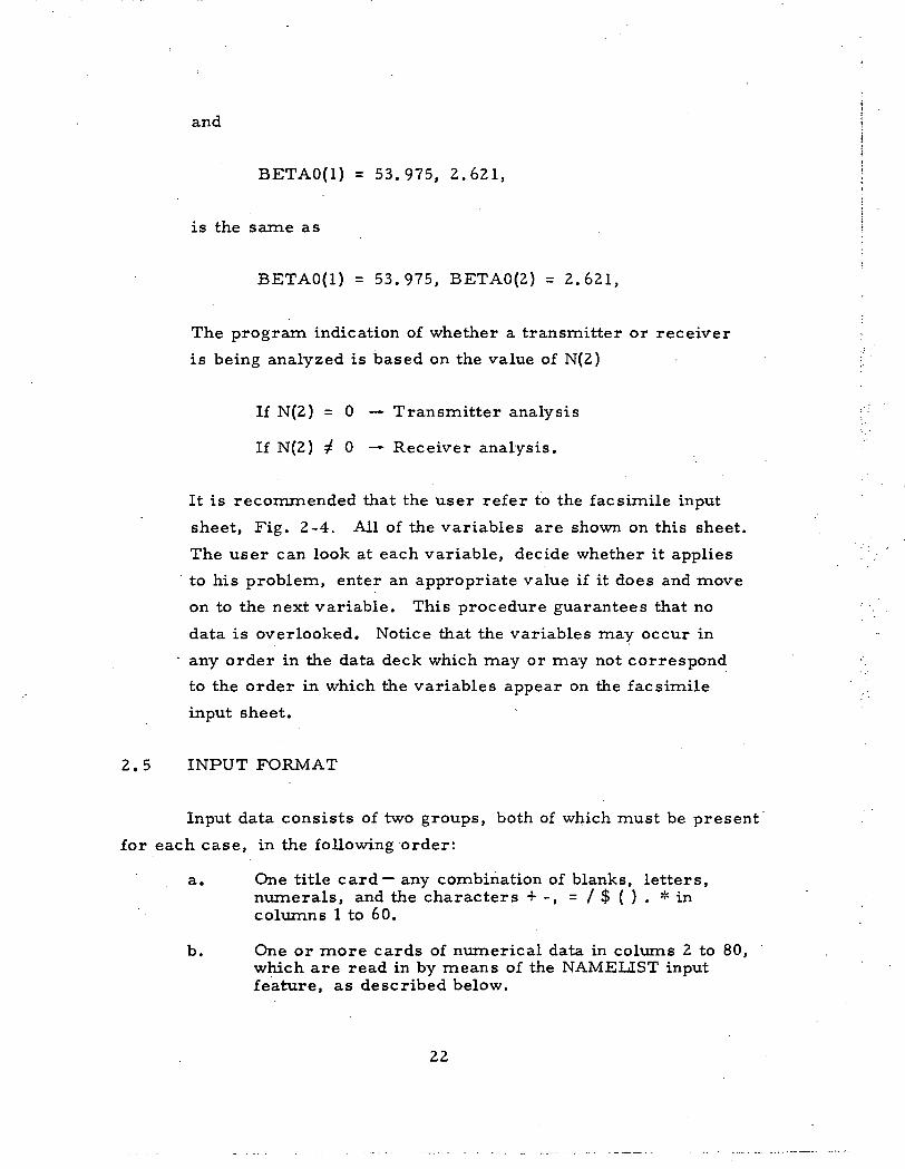
and
BETAO(l) = 53.975, 2.621,
is the same as
BETAO(l) = 53.975, BETAO(2) = 2.621,
The program indication of whether a transmitter or receiver
is being analyzed is based on the value of N(2)
If N(2) = 0 — Transmitter analysis
If N(2) 4 0 —• Receiver analysis.
It is recommended that the user refer to the facsimile input
sheet, Fig. 2-4. All of the variables are shown on this sheet.
The user can look at each variable, decide whether it applies
to his problem, enter an appropriate value if it does and move
on to the next variable. This procedure guarantees that no
data is overlooked. Notice that the variables may occur in
' any order in the data deck which may or may not correspond
to the order in which the variables appear on the facsimile
input sheet.
2.5 INPUT FORMAT
Input data consists of two groups, both of which must be present
for each case, in the following order:
a. One title card— any combination of blanks, letters,numerals, and the characters + -, = / $ ( ) . * incolumns 1 to 60.
b. One or more cards of numerical data in colums 2 to 80,which are read in by means of the NAMELIST inputfeature, as described below.
22
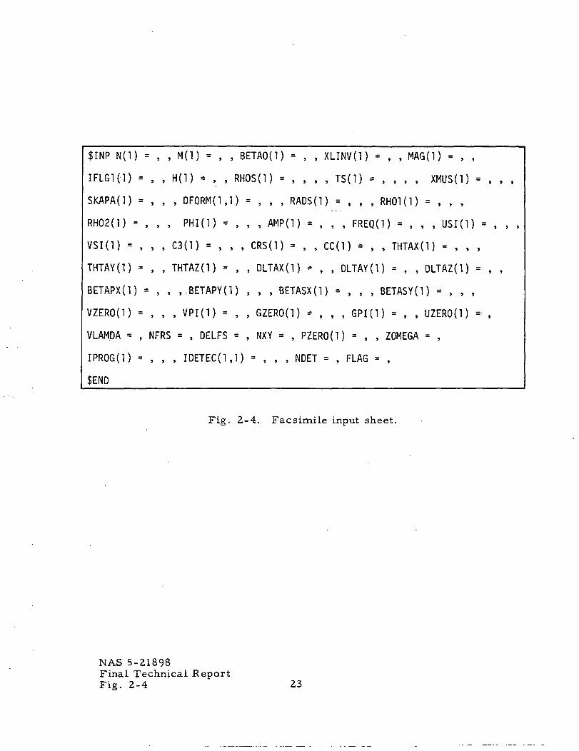
$INP N(l) = , , M(l) = , , BETAO(l) = , , XLINV(I) = , , MAG(l) = , ,
IFLGl(l) = , , H(l) = , , RHOS(l) = , , , , TS(1) = , , , , XMUS(l) = , , ,
SKAPA(l) = , , , DFORM(IJ) = , , , RADS(l) = , , , RH01(1) = , , ,
RH02(1) = , , , PHI(l) * , , , AMP(1) = , , , FREQ(l) = , , , USI(l) = , , ,
VSI(l) = , , , C3(l) = , , , CRS(l) = , , CC(1) = , , THTAX(l)
THTAY(I) = , , THTAZ(l) = , , DLTAX(l) = , , DLTAY(l) = , , OLTAZ(l) = , ,
BETAPX(I) = , , ,.BETAPY(1) , , , BETASX(l) = , , , BETASY(l) = , , ,
VZERO(l) = , , , VPI(l) = , , GZERO(l) = , , , GPI(l) = , , UZERO(l) = ,
VLAM.DA = , NFRS = , DELFS = , NXY = , PZERO(l) = , , ZOMEGA = ,
IPROG(l) = , , , IDETEC(l.l) = , , , NDET = , FLAG = ,
SEND
Fig. 2-4. Facsimile input sheet.
NAS 5-Z1898Final Technical ReportFig. 2-4 23
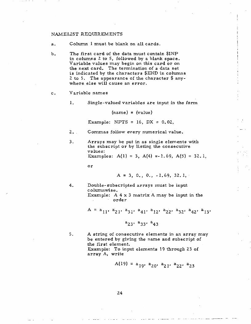
NAMELIST REQUIREMENTS j
a. Column 1 must be blank on all cards. j
b. The first card of the data must contain $INP >in columns 2 to 5, followed by a blank space. IVariable values may begin on this card or on '•the next card. The termination of a data setis indicated by the characters $END in columns \2 to 5. The appearance of the character $ any-where else will cause an error.
c. Variable names
1. Single-valued variables are input in the form
(name.) = (value)
Example: NPTS = 16, DX = 0.02,
2. . Commas follow every numerical value.
3. Arrays may be put in as single elements withthe subscript or by listing the consecutivevalues:Examples: A(l) = 3, A(4) =-1.69, A(5) = 32.1,
or .
A = 3, 0., 0., -1.69, 32. 1,
4. Double-subscripted arrays must be inputcolumnwise.Example: A 4 x 3 matrix A may be input in the
order
A = a l l » a2T a3T a41' a!2' a22' a32' a42' a!3'
a23' a33' a43
5. A string of consecutive elements in an array maybe entered by giving the name and subscript ofthe first element.Example: To input elements 19 through 23 ofarray A, write
A(19) = a , & , a , a , a
24
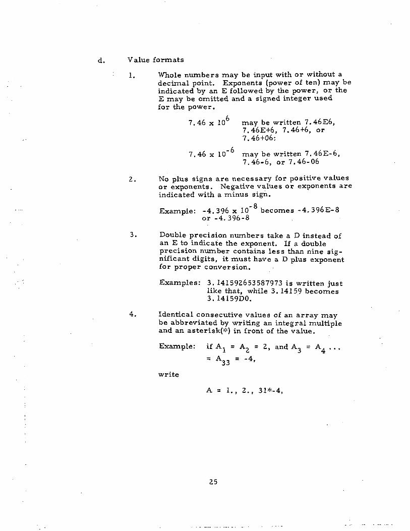
d. Value formats
1. Whole numbers may be input with or without adecimal point. Exponents (power of ten) may beindicated by an E followed by the power, or theE may be omitted and a signed integer usedfor the power.
7.46 x 10 may be written 7.46E6,7.46E+6, 7.46+6, or7.46+06:
7.46 x 10"6 may be written 7. 46E-6,7.46-6, or 7.46-06
2. No plus signs are necessary for positive valuesor exponents. Negative values or exponents areindicated with a minus sign.
Example: -4.396 x 10"8 becomes -4.396E-8or -4.396-8
3. Double precision numbers take a D instead ofan E to indicate the exponent. If a doubleprecision number contains less than nine sig-nificant digits, it must have a D plus exponentfor proper conversion.
Examples: 3. 141592653587973 is written justlike that, while 3. 14159 becomes3.14159DO.
4. Identical consecutive values of an array maybe abbreviated by writing an integral multipleand an asterisk(#) in front of the value.
Example: if A, = A- = 2, and A, = A. ...
= A33 = -4,
write
A = 1., 2., 31*-4,
25

e. Errors
1. If the $INP followed by a blank does not appearas the first punches in the first card (excludingcolumn 1), the computer will ignore that cardand continue reading, trying to find $INP in thenext cards. This process continues until $INPis found or there are no more cards. No errormessage is given if the wrong cards are beingread and rejected.
2. If a variable name is misspelled, the computerwill give an error trace, terminate execution,print the following message: "Namelist namenot found."
f. Order multiple cases
1. Variables may appear in any order.
2. Not all data need appear in any set. On suc-cessive cases where it is desired to changejust a few values, only those variables needbe input, with the rest retaining their valuesfrom previous cases.
3. Values are all zero initially, unless other-wise specified. Thus, it is necessary toinput only nonzero values. If runs arestacked, however, any data not written overwill carry over from the preceding run.
4. The same variable name may appear two ormore times in a data set. The value physicallylast in the deck will override any previousvalues. Thus, it is not necessary to repunchcards to change numbers, just place a cardwith the changed value (and variable namewith proper subscript, if any) somewherefollowing the old value.
26
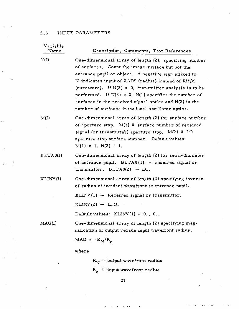
2.6 INPUT PARAMETERS
VariableName
BETAO(I)
XLINV(I)
MAG (I)
Description, Comments, Text References
One-dimensional array of length (2), specifying number
of surfaces. Count the image surface but not the
entrance pupil or object. A negative sign affixed to
N indicates input of RADS (radius) instead of RH0S
(curvature). If N(2) = 0, transmitter analysis is to be
performed. If N(2) x 0, N(l ) specifies the number of
surfaces in the received signal optics and N(2) is the
number of surfaces in the local oscillator optics.
One-dimensional array of length (2) for surface number
of aperture stop. M(l) = surface number of received
signal (or transmitter) aperture stop. M(2) = LO
aperture stop surface number. Default values:
M(l) = 1, N(2) + 1.
One-dimensional array of length (2) for semi-diameter
of entrance pupil. BETAO(l) — received signal or
transmitter. BETAO(2) — LO.
One-dimensional array of length (2) specifying inverse
of radius of incident wavefront at entrance pupil.
XLINV(l) — Received signal or transmitter.
XLINV(2) — L.O.
Default values: XLINV(l) = 0. , 0. ,
One-dimensional array of length (2) specifying mag-
nification of output versus input wavefront radius.
MAG = -RN/RQ
where
RN ^
R =
output wavefront radius
input wavefront radius
27
and the sign conventions on R , R.., are standard.
MAG(l) — Received signal or transmitter.
MAG(2) — L.O.
Default: MAG(l) = 0., 0.,
IFLG1(I) One-dimensional array of length (2) controlling location
of image (or detector).
IFIFLG1 = 0 T^ j = BF + T
IFIFLG1 = 1 T'N j = TN j + TN
where
T' , = spacing used in analysis as spacing
from surface (N-l) to image
BF = Paraxial back focus
T N _J = input value TS(N-l)
TN = input value TS(N)
IFLGl(l) — Received signal or transmitter
IFLG1(2) — L.O.
Default: IFLGl(l) = 0,0,
NOTE: For IFLG1 = 1 and TN * 0, TN_ j will not
revert to its previous value when running
consecutive cases.
H(I) One-dimensional array of length (2) specifying obliquity
in radians of input beam.
H(l) Received signal or transmitter
H(2) L.O.
Default: H(l) = 0., 0.,
28
RH0S(I) One-dimensional array of length (101) for the spherical
curvature (or base curvature of an asphere) for the I
surface when N is positive. The sign convention to be
applied to RH0S is that the curvature of a surface is
positive when the center of curvature lies to the right
of the surface.
RADS(I) One-dimensional array of length (101) for the spherical
radius (or base radius of an asphere) for the I*n optical
surface. The sign convention for RADS is the same as
that for RH0S.
N must be entered negative when data is input into this
array.
RADS(I) = 0 defines a plane surface.
TS(I) One-dimensional array (101) for the axial separation
between surface I and I + 1.
The sign convention for TS is that TS is positive for
spacings measured from left to right.
XMUS(I) One-dimensional array (101) for the index or refrac-
tion of the medium between surfaces I and I + 1.
A sign change between XMUS (I- 1) and XMUS(I) indicates
a reflection at surface I.
Default: XMUS(I) = 1.
DF0RM(J, I) Two-dimensional array (5, 101) for aspheric deformation
coefficients of the 2(J+1) power terms at surface I
. DFORM(1,I) = a
DFORM(2,I) = J
DFORM(3,I) = Y
DFORM(4,I) = 6"
DFORM(5,I) = 7
29
SKAPA(I)
The aspheric expression is
,2PQ
1 + (1 -K P2Q2)2
+ QQ4 + (3Q6 + YQ8 + . . .
where
~2 2 .. ZQ = x + y
x,y = surface intercept points
p = RH0S = base curvature
K = (1 - £ ) = conic coefficient— SKAPA
One-dimensional array (101) for conic coefficient of
surface I
where
SKAPA = K = 1 - € 2
£ = conic eccentricity
£ =
RH01(I)
RH02(I)
S2 - Sl
S, = distance from first focus to conic
S_ = distance from conic to second focus
One- dimensional array (101) for base curvature of
aspheric (acircular) cylinder. Input in addition to
RH0S(I). RH01 is used for tracing exact rays through
surface I while RH0S is used in the paraxial ray trace,
determining the first order parameters of surface I.
One- dimensional array (101). Toric rotation curvature
of surface I. RH02 used (with RH01) for exact ray
trace. RHC&S used in paraxial analysis. The optical
axis and the axes of RH01 and RH02 are mutually
orthogonal.
30
CRS(I)
CC(I)
PHI (I)
AMP (I)
FREQ (I)
One-dimensional array (101). Constant of rotational
symmetry at surface I. CRS(I) = 1., for rotationally
symmetrical surface of curvature RH01(I). CRS(I)
= -1. identifies surface I as a "perfect" surface.
Cylindrical constant. When CC(I) = 0 and CRS(I) = 0.
surface is cylinder with curvature RH01 or RH02
depending on which is nonzero. If RH01 and RH02
are nonzero, surface is toric.
One-dimensional array (101). Angular rotation of
cylindrical axes. For PHI(I)=0 the axis of the RH01
cylinder is parallel to the y axis and the axis of the
RH02 cylinder is parallel to the x axis.
One-dimensional array (101). Amplitude term for
periodic surface error function at surface I.
One-dimensional array (101). Frequency component
associated with sine function portion of periodic sur-
face error. A surface of semidiameter BETAO
will exhibit NZ sine function zeroes between the center
and the edge for
NZBETAO < FREQ < NZ + 1
BETAO
C3(I) One-dimensional array (101). Frequency component
associated with cosine function portion of periodic
surface error. A surface of semidiameter BETAO
will exhibit NC complete cycles between the center
and the edge for
2NCBETAO
2 (NC+1)BETAO
31
USI(I)
VSI(I)
DLTAX(I)
DLTAY(I)
DLTAZ(I)
THTAX(I)
THTAY(I)
THTAZ(I)
BETAPX(I)
BETAPY(I)
One-dimensional array (101). Displacement in
x direction of origin of periodic surface error at
surface I.
One-dimensional array (101). Displacement in
y direction of origin of origin of periodic surface
error at surface I.
One-dimensional array (101) for displacement Ax
of coordinate system at surface I.
One-dimensional array (101) displacement Ay of
coordinate system at surface I.
One-dimensional array (101), displacement Az of
coordinate system at surface I.
One-dimensional array (101) for angular rotation
or tilt 6x in radians around the y axis at surface I.
If THTAX(I) input greater than ITT, it is assumed
to be degrees.
One-dimensional array (101), angular rotation or
tilt 6y in radians (or degrees if 0y > ZTT) around the
x axis at surface I.
One-dimensional array (101), angular rotation in
radians (degrees if 6z > 2ir) around the z (optical)
axis at surface I.
One-dimensional array (101), semiaperture of
obscuration in x direction at surface I.
One-dimensional array (101), semiaperture of
obscuration in y direction at surface I. If both
BETAPX and BETAPY are entered, the obscuration
is rectangular. If only one is entered, the obscuration
is circular (i.e., BETAPX = 12., BETAPY = 0. , ) .
32
BETASX(I) One-dimensional array (101), semiaperture of
vignetting in y direction at surface I.
If BETASX and BETASY are both nonzero, the clear
aperture is rectangular. If only one is nonzero, the
clear aperture is circular.
NOTE: Normally, only those rays are traced which
lie inside BETASX, BETASY and outside BETAPX,
BETAPY. If anegative sign is attached to any of
the four values at surface I, the logic is reversed
so that only rays are traced which fall inside
BETAPX, BETAPY or outside BETASX, BETASY.
This produces the effect of an annular obscuration.
VZER0(I) One-dimensional array of length (2). Allows repre-
sentation of percent vignetting of upper edge of
entrance pupil. Expressed as fraction so that
VZER0 = 0.5 reduces clear aperture of upper edge
to BETAO/2. VZER0 = 0. or 1. represent no
vignetting.
VZER0(1) — Received signal (or transmitter)
VZER0(2) — L.O.
Default: VZER0(1) = 0., 0.,
VPI(I) Same as VZER0 but for lower edge of entrance
pupil.
GZER0(I) One-dimensional array (2). Entrance pupil
obscuration parameter. Distance from center of
entrance pupil to edge of upper obscuring aperture.
33
GPI(I)
UZER0(I)
VLAMDA
NFRS
GZER0(1) -» Received signal or transmitter
GZER0(2) -. L. 0.
Default: GZER0 (1) = 0., 0.,
One-dimensional array (2). Same as GZER0 but for
lower edge of obscuring aperture.
One-dimensional array (2). Radius of obscuring aperture.
Arc of radius UZER0 passes through GZER0 (concave
downward) and through GPI (concave upward). No rays
are traced below the arc through GZER0 or above the arc
through GPI. For a circular, centered obscuration
UZER0 = GZER0, UZER0 must be nonzero if GZER0
and/or GPI are entered.
UZER0(1) — Received signal or transmitter
UZER0(2) - L. O.
Default: UZER0(1) = 0., 0.,
Spectral wavelength of operation of system being
analyzed. All dimensional data (TS, BETAO, etc.) must
be in same units as wavelength.
Default: VLAMDA = 0.010611385 (mm)
Integer input specifying number of intervals or output
points for which spread function (ASF, PSF) arrays are
computed. Dimensions of spread function array
= (2-NFRS-1) x (2-NFRS-1) •
NFRS < 51.
Default: NFRS = 26
(giving spread function arrays = 51 x 51).
34
DELFS
NXY
PZER0(I)
Spread function interval size. Nominally 1/10 the Airy
disc radius. Detector parameters are specified as inte-
ger multiples of this value.
Default: DELFS + 0.61 FL10-BETAO
where FL, and BETAO are respectively the focal length
and semiaperture for the received signal or transmitter
optics.
Integer input specifying number of grid points over
entrance pupil semidiameter. The total pupil arrayis (2 • NXY + 1) x (2. NXY + 1)
NXY < 50
Default: NXY = 25
(giving pupil array = 51x51) .
Receiver— PZER0(1) = Radiant power density at entrance
pupil of received signal optics. If PZER0(1) input
negative, PZER0(1) = total radiant power incident
(uniformly) on entrance pupil. PZER0(2) = total radiant
power in truncated gaussian beam of L. O. laser.
Transmitter— PZER0(1) = total radiant power in
truncated gaussian transmitter laser beam.
Default: PZER0(1) = !.,!.,
35
Z0MEGA
IPR<Z>G(1)
IPR0G(3)
IPR0G(4)
IPRg)G(5)
IPR0G(6)
Radius of 1/e intensity point of transmitter or L.O.
gaussian laser beam.
Default-transmitter: Z0MEGA = BETAO(l)
Default-receiver: Z0MEGA = BETAO(2)
One-dimensional array of integer flags for various
program options.
Default: IPR0G(1) = 1 , 0 , 0 , 0 , 0 , 0 ,
= 0 - Paraxial analysis only
= 1 - compute receiver or transmitter quality criteria
= 0 - Pass
= 1 - Output receiver ASF arrays or transmitter PSF
array.
= 0 - Compute receiver quality criteria with detector
centered on optical axis, received signal and L.O.
beams shifted due to effect of input beam obliquity,
misalignments, IMC error, etc.
= 1 - Center received signal and L.O. chief rays on
detector
= 2 - Center respective peaks of ASF for received
signal and L.O. on detector.
= 0 - Pass
= 1 - Print un-normalized transmitter PSF
= 0 - Pass
= 1 - Print OPD (w(u, v)) arrays
= 0 - Pass
= 1 - Print pupil function
36
NDET
IDETEC(I, J)
IDETEC(I, J)
Integer input specifying number of detectors to be
analyzed.
Default: NDET = 1,
Two-dimensional array (5, 5) defining parameters of
detectors to be included in analysis.
= a, b ,c ,d , e,
I = a, b, c, d, e,
J = Detector number
IDETEC(1, J) = a = circular, rectangular flag
1 - circular detector
2 - rectangular detector
IDETEC(2, J) = b = Integer input specifying number of grid points
across x dimension of detector. Total width Sx of detec-
tor in x direction is Sx = 2-b-DELFS
IDETEC(3, J) = c = Integer input specifying number of grid points
across y dimension of detector. Total width Sy of detec-
tor in y direction is Sy = 2-c'DELFS. For circular
detector c = 0 and Sx = circular diameter.
IDETEC(4, J) = d = Integer input specifying number of grid points
by which detector center is to be displaced from the
optical axis in the x direction. Detector displacement
= Dx, and Dx = d-DELFS.
IDETEC(5, J) = e = Integer input specifying number of grid points by
which detector center is to be displaced from the optical
axis in the y direction. Detector displacement = Dy
and Dy = e-DELFS
37
Default: a = 1
b = 10
c = 0
d = 0
e = 0
NOTE: Any combination of b and d; c and e; or off-axis
chief ray shift causing the detector to fall outside the
spread function array (NFRS) will abort the run.
FLAG An integer flag used to reinitialize data. Primarily
used between consecutive runs to wipe out all data from
a previous run. This is submitted as an independent data
deck with title card, #INP card with FLAG = 1, and
$END card. Stacking this between two data decks
accomplishes the initialization for the second set of data.
2.7 INTERPRETATION OF OUTPUT DATA
The amount of output data printed is controlled by the IPR0G
flags. The system parameters as input will always be printed; the
paraxial ray traces and computed first order parameters will always be
printed. For the full transmitter or receiver analysis the full set of
quality criteria will always be printed.
a. Paraxial Data
• Entrance pupil position T(0) = , the value printed hereis the distance from the paraxial entrance pupil tothe first surface. A negative value indicates that the
- entrance pupil lies to the right of the first surface.
• TEXET — Paraxial exit pupil position, TEXIT = distancefrom surface (N-l) to paraxial exit pupil.
• XLINV — Inverse object distance as input or as computedfrom input of MAG.
• FOCAL LENGTH — computed paraxial focal length.
38
BACK FOCAL, LENGTH — computed paraxial backfocal length = distance from surface (N-l) to paraxialfocal plane.
TS (N- 1) — Spacing actually used in analysis asdistance from surface (N- 1) to image or detectorsurface. Depends on IFLG1, TS(N), etc.
FL-whenXLINV 4 0. FL = MAG/XLINV so thatan input wavefront radius at the entrance pupil ofR = L = 1 /XLINV will give an output wavefrontradius of FL.
Chief Ray Data
Field Angle — is the value input as H
Chief Ray Coordinates — x, y, z are the coordinatesof the intersection of the chief ray with the imagesurface.
Direction Cosines — 1, m, ri for chief ray in image space.
RW — Radius of reference wavefront to be used tocompute OPD values over exit pupil.
TR — Location of reference wavefront, TR = Axialdistance from surface (N-l) to reference wavefront.For axial case TR = TEXIT.
XTILT — For off-axis case, reference wavefrontmay be tilted or rotated XTILT = THTAX for refer-ence wavefront.
YTILT— = THTAY for reference wavefront.
XDISP— with tilts and decentrations, the chief raymay become a skew ray so that it does not intersectthe optical axis. XDISP is the distance from the chiefray to the optical axis at its'point of closest approach.
XDISP = DLTAX for reference wavefront.
YDISP— Same as XDISP, YDISP represents distancefrom optical axis to chief ray at point of closestapproach.
YDISP = DLTAY for reference wavefront.
39
c. Wavefront Error Information
After all the OPD (W(u, v)) values have been computed
over the reference wavefront, wavefront statistics are computed.
SI =U V
S2 =u v
STD DEV . - (f )
RMS = { Vf
• Maximum un-normalized error = WMAX
• Minimum un-normalized error = WMIN
• Maximum normalized error = WMAX/X.
• Minimum normalized error = WMIN/X.
WMAX = maximum value of W(u, v)
WMIN = minimum value of W(u, v)
• Approximate Strehl ratio = I(cr)
I(cr) = 1. - (2 -TT-STD DEV)2
d. Spread Functions - (ASF and PSF) IPROG(2) = 1. -
For the receiver analysis, selection of this option prints out the arrays
FR and FI for the received signal and the local oscillator (ASF(x, y) =
FR(x,y) + iFI (x,y)) .
labelled
"ASF (REAL), FOR RECEIVED SIGNAL" (FR1)
"ASF (IMAGINARY), FOR RECEIVED SIGNAL" (FI1)
40
"ASF (REAL), FOR LOCAL OSCILLATOR" (FR2)
"ASF (IMAGINARY), FOR LOCAL OSCILLATOR" (F12)
"PHASE" is also printed where PHASE = ARCTAN (FI/FR).
The ASF values are normalized to 100 for compactness and
the normalizing factor is printed. The ASF arrays will be (2- NFRS- 1)
x (2«NFRS-1) up to 72 x 72 beyond which only the central 72 x 72 points
will be printed.1- If the array is smaller than 36 x 36, the entire array
will be on a single page. Arrays larger than 36 x 36 will be printed
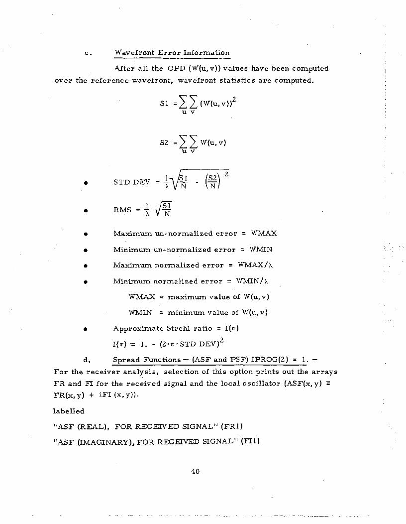
one quadrant per page. The quadrants are related as per Fig. 2-5
with the 0, 0 point in the upper left hand corner of quadrant 4.
3079-4
0,0
Fig. 2-5.Output quadrants for ASF, PSF, pupilfunction.
PSF — The PSF or intensity value for a point in an array is
PSF(x.y) = (FR(x,y))2 + (FI(x,y))2. The PSF array is printed for
the transmitter. All the comments for the ASF printout apply here.
INTERVAL — This is the spacing between adjacent ASF or PSF
points. INTERVAL = DELFS.
NUMBER INTERVALS = 2-NFRS-1
e. IPR0G(4) = 1. — This option causes the printing of the
floating point tabulation of the transmitter PSF (intensity) values.
f. IPR0G(5) = 1. — This option causes the floating point
tabulation of the OPD values to be printed.
41
g. IPROG(6) = 1. - This option prints the complex
components of the pupil function normalized to 100. As with the ASF
and PSF, the output may include only the central 72 x 72 of a larger
array.
2.8 COORDINATE - SIGN CONVENTION SUMMARY
The coordinate system for ray tracing is a local coordinate sys-
tem where the vertex of the surface being traced is the origin. The
spacing TS combines with any misalignment parameters to transfer
the coordinate system from surface to surface with the ray. Some
key points regarding sign conventions and coordinates are summarized
here.
• Surface parameters — A surface parameter with apositive sign causes the surface to be deviated tothe right of the tangent plane, hence the negativesign indicates a deviation to the left of the tangentplane. Some of those parameters are:
RH0S, RH01, RH02, RADS, DF0RM, AMP.
• Spacing — TS. A positive value for TS(I) specifiesthat surface I + 1 lies to the right of surface I.
• Finite object— nonuniphase input beam. A positivevalue for XLINV indicates that the entrance pupillies to the right of the object point. The input wave-front is thus divergent. For MAG input positive fora system with a positive focal length, the inputwavefront is divergent and the exiting wavefront isconvergent.
• H-input beam obliquity — A positive H indicates aninput beam incident on the entrance pupil from belowthe optical axis.
• Misalignments - DLTAX, DLTAY, DLTAZ, THTAX,THTAY, THTAZ- refer to Section 4. 6.
• Detector— The optical axis is the reference here.For a centered system with no input beam obliquity,the detector, the received signal and the L. O. beamwill be centered on the optical axis. If there is aninput beam obliquity or misalignment in either the
42
received signal or the local oscillator, that beamwill be shifted from the center of the detectorwhile the other beam remains centered. Thedetector will always remain centered regardlessof the shift in the beams unless the IPR0G(3)option is invoked or the detector is displacedvia IDETEC(4, J) and/or IDETEC(5, J). Noticethat IPR0G(3) centers the spread functions onthe detector while IDETEC(4 and 5, J) shift thedetector with respect to the optical axis withoutchanging the location of the beams.
2.9 SAMPLE CASES
Computed results are included for four sample cases. There
are two transmitter cases and two receiver cases. The descriptions
of these cases are as follows:
a. "TRANSMITTER TEST CASE", Appendix A - This very
simple case is an example of an analysis using a "perfect surface".
Surface No. 1 is a dummy surface, surface No. 3 is the image surface
and surface No. 2 is the perfect imaging surface. For this perfect
system, the focal length and back focal length are equal at 100 mm.
The transmitter quality criteria are determined at the (Fraunhofer)
focal plane. The overall transmitter efficiency is 92% rather than
approaching 100% because of the gaussian beam.
An examination of the data deck for this case would indicate
the presence of data for a complete receiver. The transmitter analysis
results from setting N(2) = 0.
b. "TRANSMITTER TEST CASE No. 1", Appendix B - This
system consists of a meniscus lens represented by surfaces No. 2 and
No. 3 and a paraboloidal mirror represented by surface No. 5. Sur-
face No. 1 is a dummy located at the position of the laser input; surface
No. 4 is a dummy at the mutual focus of the meniscus and paraboloid.
The combination of the meniscus and paraboloid produces a perfectly
collimated beam so that surface No. 6 is a perfect surface chosen to
focus the beam at a distance of 8 km (back focal length —
8.00178987- 10 mm). The laser beam defaults to a total power of
43
1 W. The 1/e radius is specified to be 0.925 mm (Z0MEGA = 0.925)
and the far field intensity is sampled in increments of 50 mm (DEL.FS
= 50. 0). The reference wavefront has a radius of 7. 9 km
(RW = 7. 93148013-10 mm) and is located 70 m to the right of surface
No. 6 (TR = 7. 03097397- 10 ). The quality criteria are essentially
self-explanatory with the added comment that the apparently low value
for overall transmitter efficiency is due to the disparity between the
1/e radius (0.925 mm) and the truncation radius (BETAO = 2.25).
c. "RECEIVER TEST CASE No. 1", Appendix C - The
received signal optics for this system are for a real system. The
local oscillator optics is a perfect surface of aperture and focal length
to give an Airy disc about five times the diameter of that for the
received signal. The peak value for the ASF(REAL) for the received
signal (FR1) is 1304. 5 while the peak value for the ASF (Imaginary) for
the received signal (FI1) is 600. 1 indicating that the peak intensity is
2.062. 10 and that the focus can be improved (to reduce FI1). The
ASF values for the local oscillator indicate good focus so that the peak
intensity will be 2. 0042 = 4. 0160.
The ASF arrays are output for the two beams allowing an examina-
tion of the respective distributions. The FI arrays are converted to
phase and exhibited since default conditions are relied on for the quality
criteria. They are based on a circular detector of diameter equal to
that of the Airy disc for a system of clear, uniformly illuminated
aperture, and relative aperture = 8. 0.
d. "RECEIVER TEST CASE No. 2", Appendix D- This data
is for a typical set of received signal and local oscillator optics. The
quality criteria are determined for the default case plus three other
detectors:
(1) Detector No. 1 — Default case— circular, centereddetector with diameter equal to the Airy disc.
(2) Detector No. 2 — Square, centered detector withsides equal'to the diameter of the Airy disc.
44

(3) Detector No. 3 — Circular detector with samedimensions as Detector No. 1 but shifted from thebeam center by a distance equal to the radius ofthe Airy disc.
(4) Detector No. 4— Square detector with the samedimensions as Detector No. 2, but shifted frombeam center by the Airy disc radius.
45
S E C T I O N I I I
SAMPLE SYSTEM ANALYSIS
The system chosen for exercising this computer program is the
optical mechanical subsystem (OMSS) developed for NASA under con-
tract NAS 5-21859. This package is intended as an engineering model
of a spaceborne data link and is one of the most advanced systems
designed specifically for heterodyne communications work. The system
has been designed and analyzed using existing optical computer programs
and represents a nearly perfect optical system. As will be seen, the
excellent performance predicted by a conventional program, ACCOS V
is confirmed by LACOMA. Since the performance is nearly perfect,
the differences between LACOMA and conventional programs are masked.
An example of a less perfect system is presented at the end of this
section to illustrate the advantages of LACOMA over programs that
optimize intensity.
The OMSS consists of two focusing reflective surfaces, a para-
bolic primary and an elliptic secondary. This particular configuration
provides essentially perfect performance when properly aligned, and,
even in the presence of reasonable tilts and decentrations, performance
is still excellent.
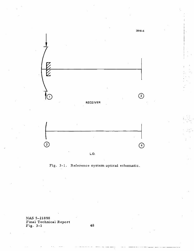
The analysis was carried out in three steps. First, a reference
case using the same size optics with the same obscurations but with a
"perfect" surface in the receive and the L. O. paths was analyzed to
provide a measure of the best possible performance under the given
restraints. The configuration of this system is shown in Fig. 3-1; the
optical input data and the results are listed in Table 3-1.
Preceding page blank
47
RECEIVER
3079-5
L.O.
©
Fig. 3-1. Reference system optical schematic.
NAS 5-21898Final Technical ReportFig. 3-1 48
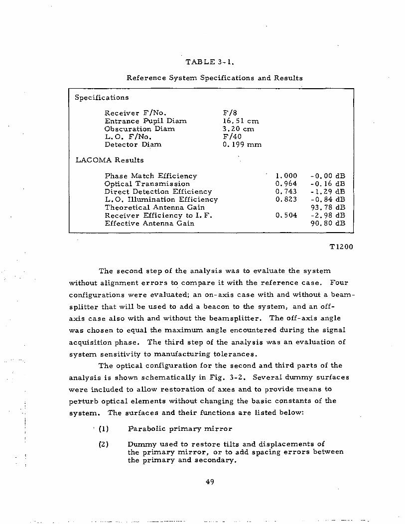
TABLE 3-1.
Reference System Specifications and Results
Specifications
Receiver F/No. F/8Entrance Pupil Diam 16.51 cmObscuration Diam 3 . Z O cmL.O. F/No. F/40Detector Diam 0. 199 mm
LACOMA Results
Phase Match EfficiencyOptical TransmissionDirect Detection EfficiencyL.O. Illumination EfficiencyTheoretical Antenna GainReceiver Efficiency to I. F.Effective Antenna Gain
- i .ooo0.9640.7430.823
0.504
-0.00 dB-0. 16 dB-1.29 dB-0.84 dB93.78 dB-2.98 dB90.80 dB
T1200
The second step of the analysis was to evaluate the system
without alignment errors to compare it with the reference case. Four
configurations were evaluated; an on-axis case with and without a beam-
splitter that will be used to add a beacon to the system, and an off-
axis case also with and without the beamsplitter. The off-axis angle
was chosen to equal the maximum angle encountered during the signal
acquisition phase. The third step of the analysis was an evaluation of
system sensitivity to manufacturing tolerances.
The optical configuration for the second and third parts of the
analysis is shown schematically in Fig. 3-2. Several dummy surfaces
were included to allow restoration of axes and to provide means to
perturb optical elements without changing the basic constants of the
system. The surfaces and their functions are listed below:
' (1) Parabolic primary mirror
(2) Dummy used to restore tilts and displacements ofthe primary mirror, or to add spacing errors betweenthe primary and secondary.
49
3079-6
Qj)(JQ) r
(9)
(?
L.O. SCHEMATIC
RECEIVER SCHEMATIC
Fig. 3-2. OMSS optical schematic.
NAS 5-21898Final Technical ReportFig. 3-3 50
(3) Elliptical secondary mirror
(4) IMC mirror
(5) Dummy to restore the optical axis to 90° afterreflection from the IMC. The sum of the tiltangles of surfaces 4 and 5 must always equal90°.
(6) Aperture stop
(7) First beamsplitter surface
(8) Second beamsplitter surface
(9) Dummy to restore tilted axis introduced by surfaceNo. 7
(10) Dummy to restore offset between optical axis andchief ray caused by the beamsplitter
(11) Detector plane for receiver pathr
(12) L. O. perfect surface and aperture stop
(13) Detector plane for L.O.
The constants to describe each surface for the nominal on-axis
case are listed in Table 3-2. These values were determined during the
OMSS design phase, and have been optimized for best Strehl ratio
(diffraction focus). Note that there are three reflective surfaces in
the system; both the refractive index and the direction of propagation
(spacing) reverse sign at these surfaces.
Local Oscillator — At the time of this analysis, there was no
final design data for the L.O. Accordingly, to avoid introducing
degradation from this source, the basic design data was used to gen-
erate a "perfect" L.O. The planned L.O. will operate as a f/40 system
with a gaussian beam distribution truncated at the 1/e points, and
with no central obscuration. A perfect L.O. that meets these criteria
is also shown in Fig. 3-2, and is specified in Table 3-2.
Figure 3-3 shows a printout of the data deck as it appeared after
being input to the computer. Additional parameters shown in Fig. 3-3
are defined in Section II.
51
TABLE 3-2.
Input Data for Nominal OM Subsystem Surfaces
Surface
Primary
Dummy
Secondary
IMC
Dummy
Stop
Beamsplitter
Beamsplitter
Dummy
Dummy
Detector
Lens /Stop
Detector
No.
1
2
3
4
5
6
7
8
9
10
11
12
13
RadiusRADS
-820.0
0
141.80175
0
0
0
0
0
0
0
0
400
0
SpacingTS
( - )O
-502. 90985-
133.44387
(-)O
-12. 7
-98.425
-2
( - ) o
-54.6358
( - )O
( - ) O
400
0
IndexXMUS
-1
-1
1
-1
-1
-1
-4. 00062
- 1
-1
-1
-1
1
1
ObscurationBETAPX
16
Surface ModificationsCRS
- 1
SKAPA
0
]
0. 71736
1
1
I
1
1
1
1
1
1
1
TiltsTHTAY
0
0
0
-0. 7854
-0. 7854
0
0.7854
0
-0 .7854
0
0
0
0
DisplacementsDLTAY
0.25396
Entrance PupilRadius BETAO
82. 55
5
T1201
All lengths in millimeters, angles in radians

0!-1 S U B S Y S T L - ' - i , NO O F F S E T S :1R TILTSJ I M Pp<?TAn<i)=8i.'.55,5., "ZERO ( 1) =-i. ,1., IFiGl<1)=1,IPROG (1) =1,0,2,
-ll»-2« X1US(!)=-!. ,-1. ,1. ,3*-l.,-<*.G30620,-l.,3*-l.,M(l>=6»12»
T S ( 1 ) = C. , - • > ? ? . 9 J96? : , 1 3 3 . ^ ^ 3 ^ 7 , j . ,-12. 7,- 98 .^+2 5, -2. ,u. , -5U.6 35T S ( 1 2 1 = i * C v , . ,L . , R a C ' S < l 2 ) =•»•- -3. « J . , 3 R S ( 1 2 ) = -1., X M U S f 12) =2*1. ,0£LFS- '» . l ' * i657£-3 , N D E T - 1 , I OciT EC (1,1) = 1, 2*, 3*0 ,T H T A Y ( t » ) = 2 » -T H T A Y ( 7 ) = .7 --J
, 2 * 0 . ,
Fig. 3-3. Input deck for OM system.
NAS 5-21898Final Technical ReportFig. 2-4 53
The results for the runs without alignment errors are shown in
Table 3-3. The results show that the aberrations caused by off-axis
operation and the astigmatism caused by the beamsplitter are both
negligible. (In this table the overall efficiency to the i.f. is shown in
dB degradation below the theoretical maximum antenna gain, and is
also normalized to the results of the reference case. )
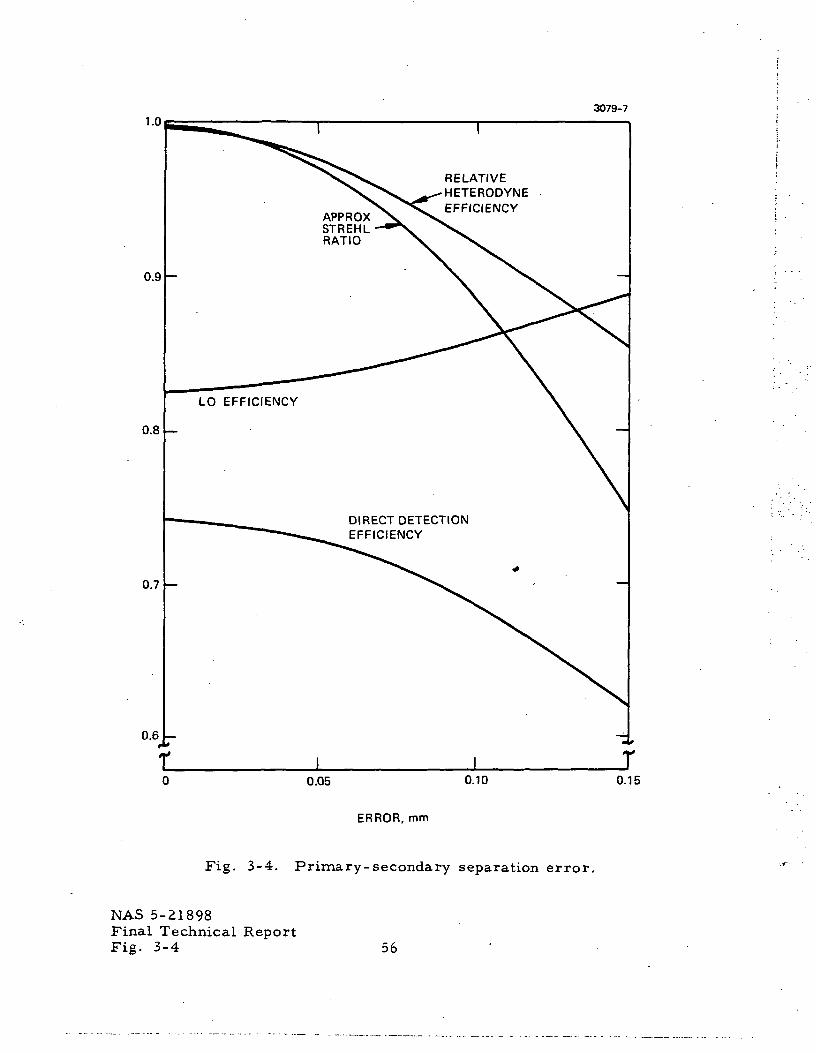
For the third step of this analysis, the distortions introduced
into the OMSS were selected to allow comparison with the analysis
conducted using ACCOS V as listed in the design report for the OMSS.
Four perturbations were analyzed:
(1) The primary-secondary spacing was varied
(2) The detector was displaced from the focal plane
(3) The primary mirror was transversely displaced
(4) The primary mirror was tilted.
The results are presented graphically in Figs. 3-4 through 3-7.
For the first two cases where the evaluation is conducted on-axis, the
results are directly comparable to those obtained using ACCOS V. The
plots show Strehl ratio, normalized heterodyne efficiency, direct
detection efficiency, and local oscillator efficiency. There are several
interesting results:
(1) Because the local oscillator has been spread out bythe f/40 optical system, the amplitude profiles ofthe L.O. and received signal tend to become moreclosely matched as the received signal is defocused,thereby increasing the local oscillator efficiencyand partially compensating the loss in signal power.
(2) Heterodyne efficiency is not as sensitive to focus asis the Strehl ratio, partially because of the aboveobservation.
(3) The region around the focal plane of the detectorwould be symmetrical in the absence of aberrations.The aberrations that are present cause a slightasymmetry in the Strehl ratio, which is barelyevident on the curves. However, the heterodyneefficiency shows amuch greater asymmetry,implying that small aberrations affect the phaseof the signal more than the amplitude.
54
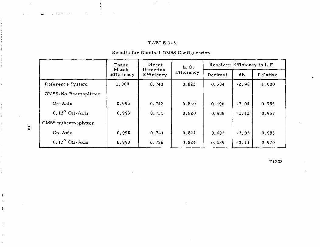
TABLE 3-3.
Results for Nominal OMSS Configuration
Reference System
OMSS- No Beamsplitter
On- Axis
0. 13° Off -Axis
OMSS w /beamsplitter
On -Axis
0.13° Off- Axis
PhaseMatch
Efficiency
1.000
0.996
0.993
0.990
0.990
DirectDetectionEfficiency
0.743
0.742
0.735
0.741
0.736
L.O.Efficiency
0.823
0.820
0.820
0.821
0.824
Receiver Efficiency to I. F.
Decimal
0.504
0.496
0.488
0.495
0.489
dB
-2.98
-3.04
-3.12
-3.05
-3. 11
Relative
1.000
0.985
0.967
0.983
0.970
U1(Jl
T1202
3079-71.0
0.9
0.8
0.7
RELATIVEHETERODYNEEFFICIENCY
APPROXSTREHLRATIO
0.6 -»*•
r
DIRECT DETECTIONEFFICIENCY
0.05 0.10 0.15
ERROR, mm
Fig. 3-4. Primary-secondary separation error.
NAS 5-21898Final Technical ReportFig. 3-4 56
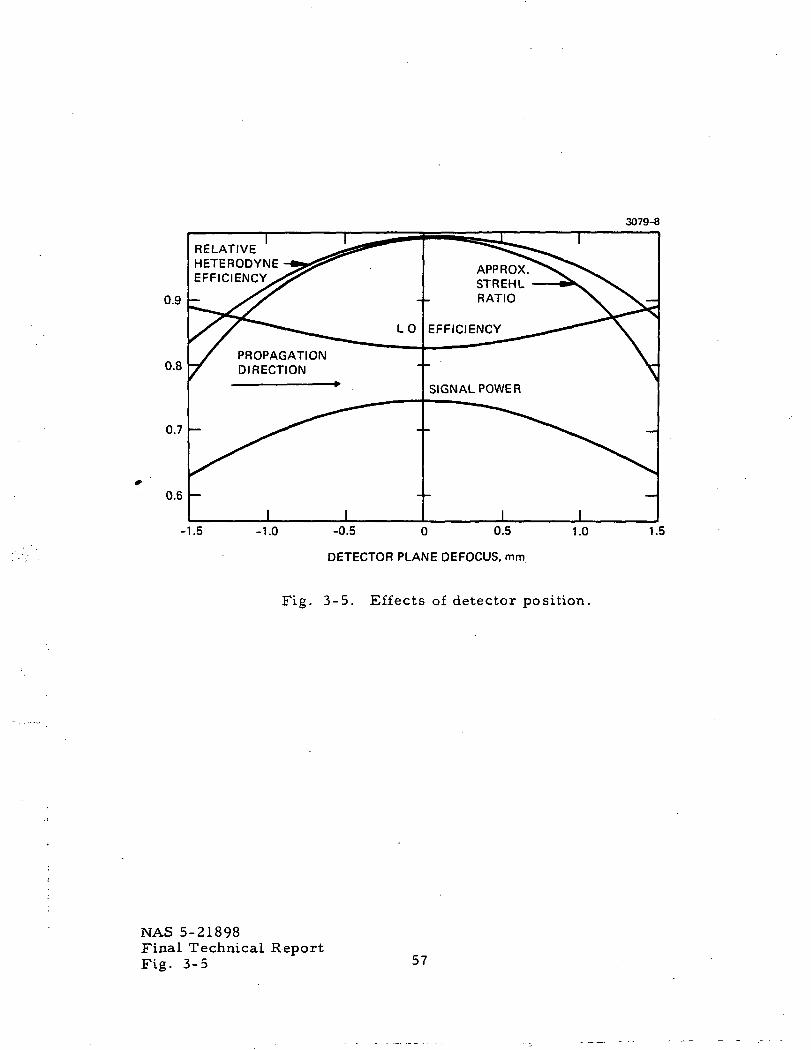
3079-8
RELATIVEHETERODYNEEFFICIENCY
APPROXSTREHLRATIO
EFFICIENCY
PROPAGATIONDIRECTION
SIGNAL POWER
0.7 -
0.6 -
-1.5 -0.5 0 0.5
DETECTOR PLANE DEFOCUS, mm
Fig. 3-5. Effects of detector position.
NAS 5-21898Final Technical ReportFig. 3-5 57
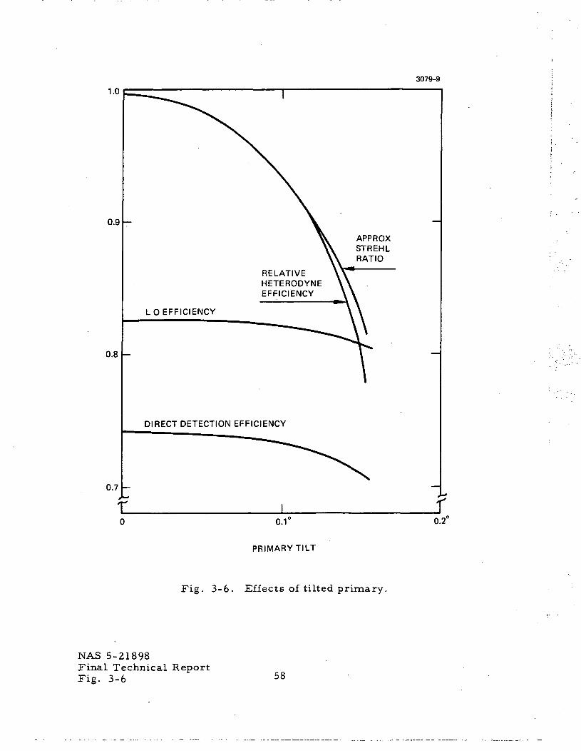
3079-9
1.0
0.9
0.8 -
0.7 -*-•r_
RELATIVEHETERODYNEEFFICIENCY
APR R OXSTREHLRATIO
DIRECT DETECTION EFFICIENCY
I r0.1°
PRIMARY TILT
0.2°
Fig. 3-6. Effects of tilted primary.
NAS 5-21898Final Technical ReportFig. 3-6 58
1.03079-10
0.9
0.8
0.7
DIRECTDETECTIONEFFICIENCY
APPROXSTREHLRATIO
RELATIVEHETERODYNEEFFICIENCY
0.5 1.0
PRIMARY DECENTRATION, mm
Fig. 3-7. Effects of primary offset.
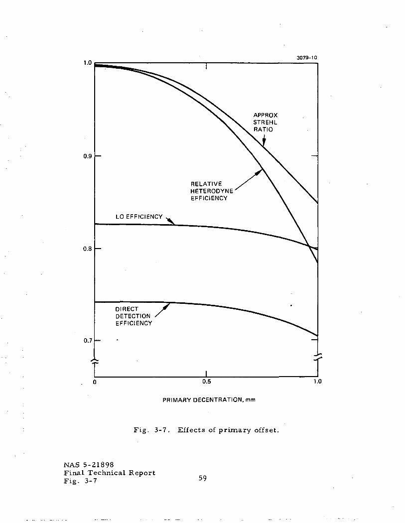
NAS 5-21898Final Technical ReportFig. 3-7 59
For cases 3 and 4 where the primary has been tilted or
displaced, the results cannot be compared directly with previous results
due to differences in methods used to evaluate the system. For the
L.ACOMA runs, the input beam was introduced along the undisturbed
optical axis and the IMC was adjusted to place the chief ray of the
received signal onto the detector center as would occur during the track
mode in the operating system. The values for IMC correction were
determined by paraxial ray trace using a desk calculator. The LACOMA
option to place the peak intensities of the two beams on the center of
the detector was selected to eliminate residual errors in IMC position
and to compensate for peak shift due to off-axis aberrations. An alter-
native approach leaves the IMC centered and compensates for the
angular displacement by evaluating a received signal from an off-axis
location. The aberrations caused by the first approach are more
severe, as is evident if the Strehl ratios in Figs. 3-6 and 3-7 are com-
pared with corresponding figures in the OMSS design report.
For these cases, as shown in Figs. 3-6 and 3-7, the heterodyne
efficiency falls off more rapidly than the Strehl ratio. This result is
not unexpected, as the heterodyne signal is more sensitive to wavefront
tilt, thus the phase match efficiency suffers. Also of interest is the
L.O. illumination efficiency which decreases for these cases, thus
adding to the degradation.
Overall, the results of this analysis tend to confirm the con-
clusions reached in the OMSS design report. The heterodyne signal
has been shown to be more sensitive to alignments that cause angular
errors than those that cause only defocusing. This result is beneficial
to the OMSS, since the primary-secondary spacing is the most difficult
parameter to control.
Other Analyses
The LACOMA program has been used to analyze several other
problems of interest; two of these are summarized here.
60
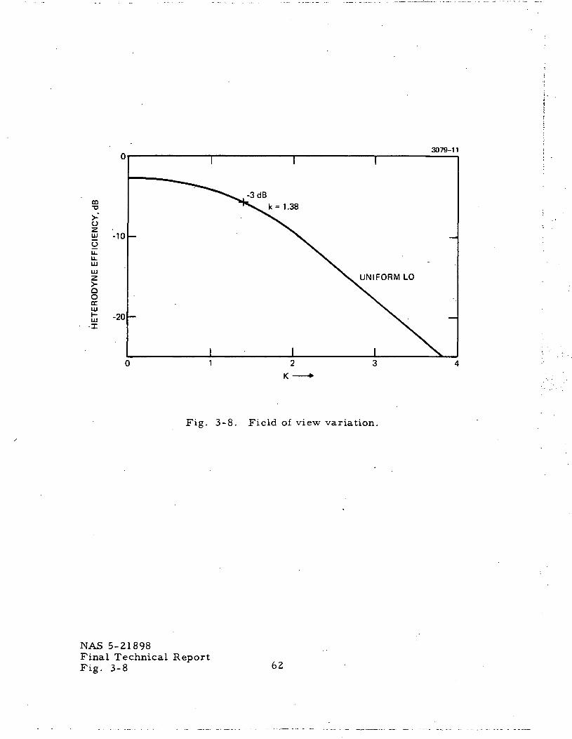
Field of View — The nominal field of view of a heterodyne
receiver has been generally considered to be k\/d, where d is the
receiver aperture diameter, and k is a constant dependent upon the
illumination factor, detector size and definition of field of view. To
evaluate k for a round detector equal in diameter to the Airy disc,
LACOMA was used with a perfect system and a series of detectors
spaced sequentially at varying distances from the optical axis..
Figure 3-8 shows the results for a uniform L.O. illumination. From
this curve, the full field of view to the 3 dB points implies that k should
be 1.38 for the uniform case.
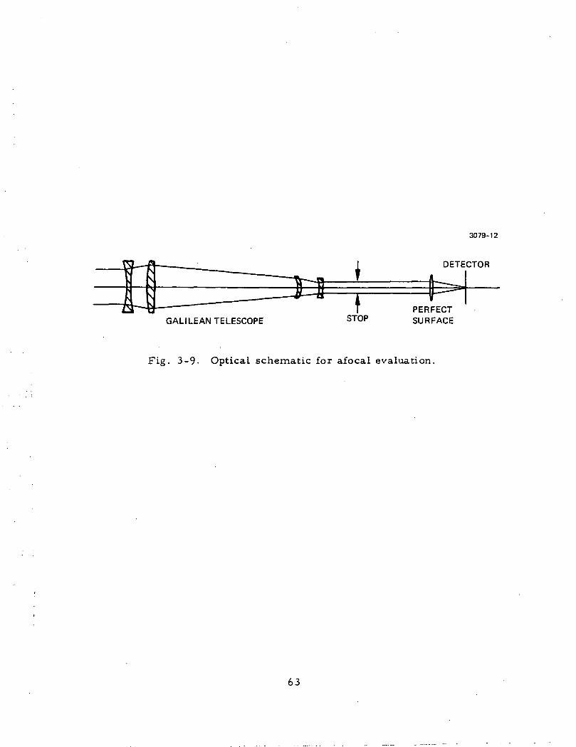
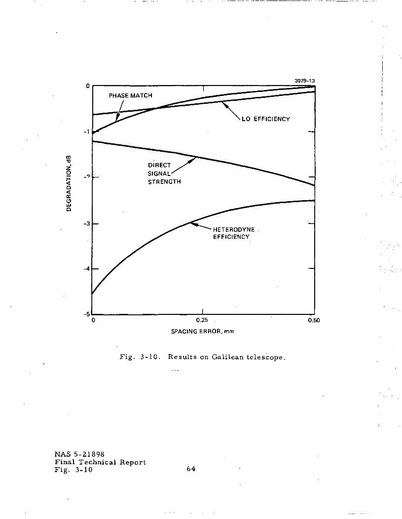
Germanium Galilean Telescope — A four-element telescope
configuration meant for use in a 10.6-^.m heterodyne system is shown in
Figure 3-9. This telescope was designed for maximum Strehl ratio,
using existing design programs. (This particular telescope has suf-
ficient spherical aberration in this configuration to reduce the Strehl
ratio to about 0. 7. ) Since this system was designed as an afocal sys-
tem, a perfect surface was introduced into the afocal beam to provide
a focal plane for evaluation, and a perfect f/40 L.O, was also selected.
The lens system was evaluated, using the predicted optimum spacings,
to determine the degradation caused by the spherical aberrations; also,
with the spacings between the first and second elements increased by
0.25 and 0.5 mm to ascertain the effects of spacing tolerances. The
results, shown in Figure 3-10, were unexpected; the overall efficiency
increased from -4. 55 dB to -2. 58 dB, which is better than the -2. 74 dB
expected from a perfect system with a uniform L.O. This result can be
explained by reference to the phase match efficiency and the L.O.
illumination efficiency. Both of these values have increased sig-
nificantly from the nominal position, even though the total signal power
has dropped. This means that at a location significantly away from the
best energy focus, the wavefront is nearly plane and the energy dis-
tribution is more uniform. Thus, in the presence of significant aber-
rations, optimum performance for a heterodyne system does not neces-
sarily correspond to that for a direct detection system. LACOMA is
the first program to put a quantitative value on this phenomena.
61
3079-11
m•o
O
w -10
UJ
ooDCUJI— onUJ ^u
• I
-3dBk=1.38
UNIFORM LO
Fig. 3-8. Field of view variation.
NAS 5-21898Final Technical ReportFig. 3-8 62
3079-12
DETECTOR
GALILEAN TELESCOPE STOPPERFECTSURFACE
Fig. 3-9- Optical schematic for afocal evaluation.
63
3079-13
-1
m•a
CCC3
-3
-5
DIRECTSIGNALSTRENGTH
HETERODYNEEFFICIENCY
I
0.25
SPACING ERROR, mm
0.50
Fig. 3-10. Results on Galilean telescope.
NAS 5-21898Final Technical ReportFig, 3-10 64
S E C T I O N IV
DETAILED PROGRAM DESCRIPTION
Upon reading the input data, the program determines whether
it is to execute a transmitter analysis or receiver analysis based on the
input of one or two sets of optical data. Specifically, it checks whether
values are entered for N(l) and N(2) which identify the number of sur-
faces in the two sets of data for received signal optics and local oscil-
lator optics, respectively. If N(2) = 0, then a transmitter analysis is
performed. In addition to the surface number parameter, many of the
other system parameters are two-element arrays; e.g., M(l) = surface
number of aperture stop for received signal (or transmitter) optical
train while M(2) = surface number of aperture stop for local oscil-
lator optical train as is the case for H(l), H(2), FL(1), FL(2), etc'.
As most of the computations to be discussed are performed identically
for transmitter, receiver, and local oscillator, the subscript notation
will be omitted except where confusion might arise and the distinction
between transmitter and receiver will be omitted except for those
computations unique to a given case.
4. 1 FIRST ORDER PARAMETERS
Two paraxial rays are traced through the optical trains to deter-
mine the first order parameters of the particular optical train. These
parameters are:
a. Paraxial entrance pupil position T is the distancefrom the paraxial entrance pupil to the first opticalsurface.
b. Paraxial exit pupil position TEXIT or TR is thedistance from the last optical surface (surface N-1)to the paraxial exit pupil.
65
c. Inverse object distance XLINV or L. is the inverseof the distance from the object plane to the paraxialentrance pupil.
d. Focal length
e. Back focal length, which is the distance from the (N- 1)surface to the paraxial focal surface.
f. TS(N-l) is based on the input data and control param-eters, and is the spacing actually used in the analysisas the back focus.
g. Paraxial Computations are where the two paraxialrays are traced with starting values at the first sur-face of the optical train.
P0 = input
b = 0.o
ao = 1/(3o
a = 0.o
With this data as input the two paraxial rays are traced using
J3 = p + b . t ,/V (4-1)* s ' s - l s - 1 s - l / h s - l
as-l
as = as-l
The parameters of these paraxial rays are illustrated in Fig. 4-1.
The data for the paraxial rays at the first surface, the aperture stop,
and at the rear surface are then used to compute the desired first
order parameters. This data is designated as follows:
66
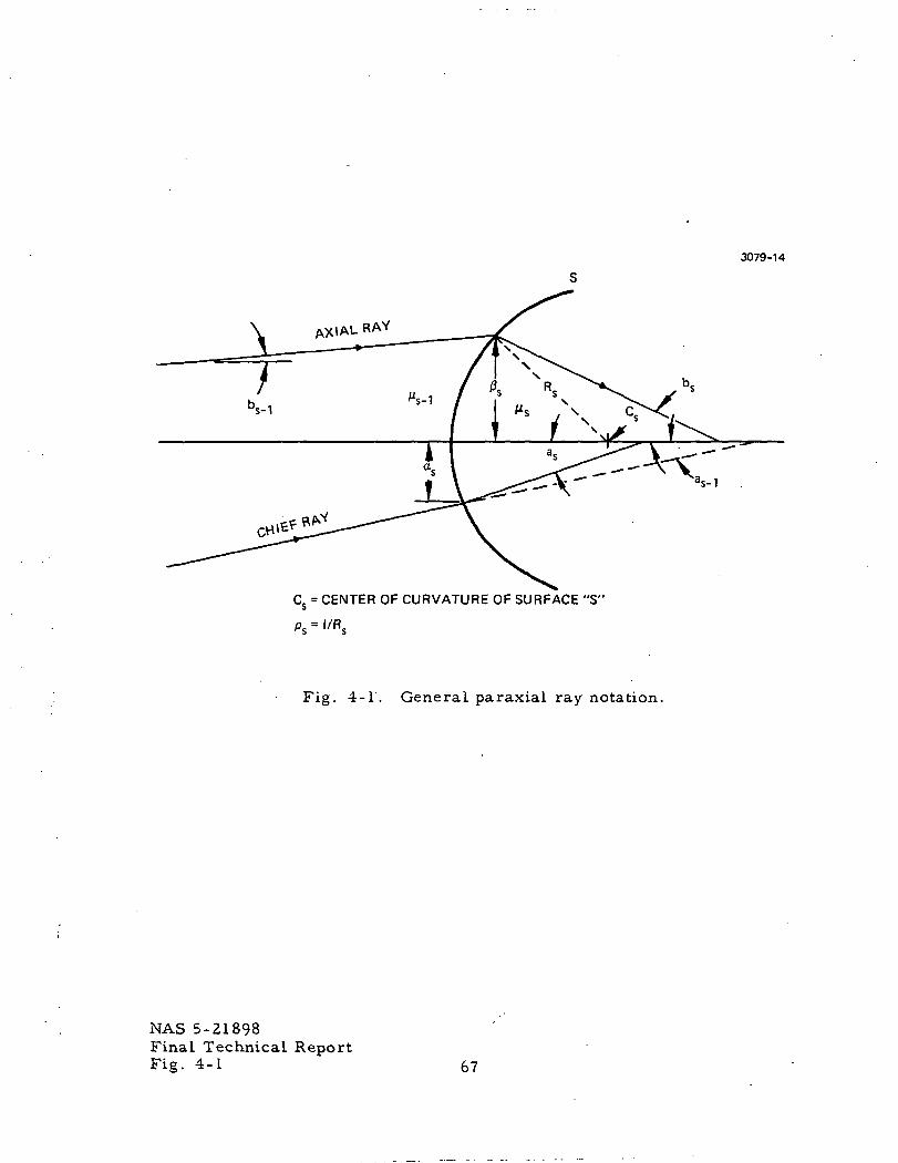
3079-14
Cs = CENTER OF CURVATURE OF SURFACE "S"
Fig. 4-1. General paraxial ray notation.
NAS 5-21898Final Technical ReportFig. 4-1 67
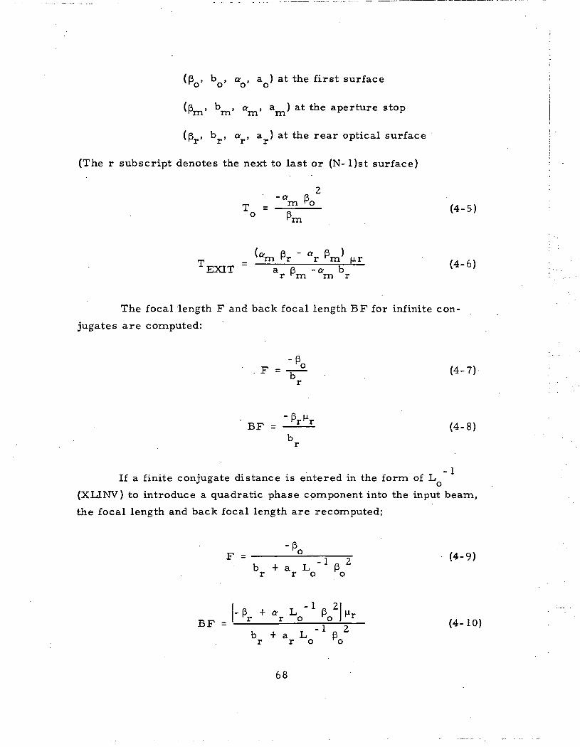
(B , b , a , a ) at the first surfaceo o o o
*Pm' bm' °m' &m^ at the aPerture st°P
(3 , b , a , a ) at the rear optical surface
(The r subscript denotes the next to last or (N- l)st surface)
(4.5)
(a R - a (3 )T
m Pr r m_EXIT a B -a br rm m r
The focal length F and back focal length BF for infinite con
jugates are computed:
(4-7)
r rBF = — Z-^- (4-8)br
If a finite conjugate distance is entered in the form of L
(XLJNV) to introduce a quadratic phase component into the input beam,
the focal length and back focal length are recomputed;
F =b + a Lr r o
-(3 + a L ~* B 2Lr
B F = l — ^ r—^ j^-4 (4-10)b + a L B
r r o o
68
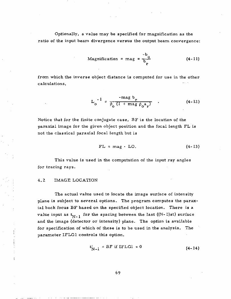
Optionally, a value may be specified for magnification as the
ratio of the input beam divergence versus the output beam convergence:
-bMagnification = mag = -r— (4-11)
r
from which the inverse object distance is computed for use in the other
calculations,
_ -magLo pQ U + mag (3oarJ
Notice that for the finite conjugate case, BF is the location of the
paraxial image for the given object position and the focal length FL is
not the classical paraxial focal length but is
FL = mag • LO. (4-13)
This value is used in the computation of the input ray angles
for tracing rays.
4.2 IMAGE LOCATION
The actual value used to locate the image surface of intensity
plane is subject to several options. The program computes the parax-
ial back focus BF based on the specified object location. There is a
value input as t-. , for the spacing between the last ((N-l)st) surface
and the image (detector or intensity) plane. The option is available
for specification of which of these is to be used in the analysis. The
parameter IFLG1 controls this option.
= 0 /,,
69
*N-1 = *N-1
where
t,^ i is the value to be used in the analysis.
Additionally, the value t~, which is usually ignored since it has
no meaning, can be used to specify an incremental shift of the image
location. Thus, the value of t., is always added to the back focus or
image distance.
tN_1 = BF + tN if IFLG1 =0 (4-14a)
t N _ j = t N _ j + tN if IFLG1 = 1 (4-15a)
For example, if it is known that the best focus for a given sys-
tem is 0.001 from the paraxial focus, the program can compute the
paraxial back focus very accurately and then shift by 0. 001 to the posi-
tion of best focus. The value of t-, , thus determined is printed out as
TS (N-l).
4.3 RAYTRACE-OPD
The LACOMA ray trace constitutes an optimal combination of
accuracy and speed of computation. The ray trace equations are the
result of many years of development, and permit the trace of both
meridional and skew rays through any surface which is continuous and
analytic.
Notation— (Figure 4-2). A given ray is described by the
parameters X , Y , Z , 1 , m and n . X , Y and Z are the* s s s s s s s s scoordinates of the point of intersection of the ray with surface "s". The
origin of the coordinate system is at the vertex of the surface. The
Z axis is the optical axis, the Y axis the meridional axis and X the
skew axis. The optical direction cosines of the ray exiting surface "s"
70
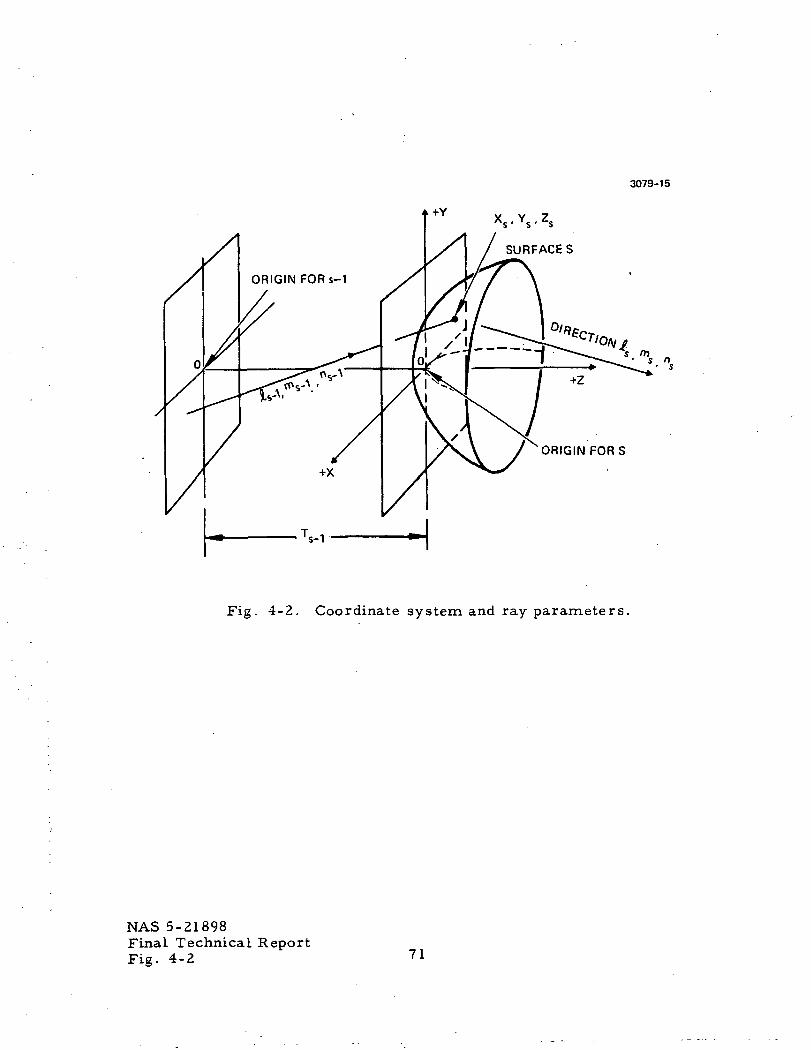
3079-15
ORIGIN FORS
Fig. 4-2. Coordinate system and ray parameters.
NAS 5-21898Final Technical ReportFig. 4-2 71
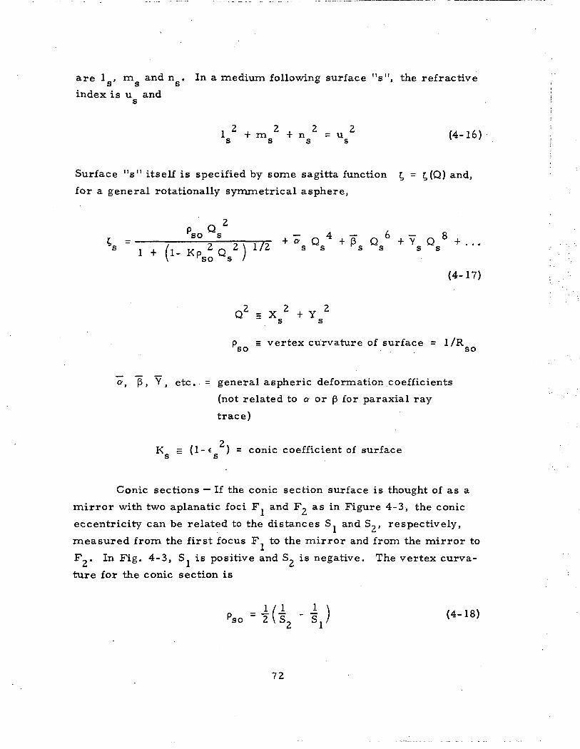
are 1 , m and n . In a medium following surface "s", the refractives s sindex is u and
s
! 2 + m 2 + n 2 = u 2 (4-16)s s s s v
Surface "s" itself is specified by some sagitta function t, = £,(Q) and,
for a general rotationally symmetrical asphere,
1 217^s2
[1- Kp L Q\ rso
(4-17)
Q2 = X 2 + Y 2
s s
p = vertex curvature of surface = 1/Rso so
en, p, Y, etc. = general aspheric deformation coefficients
(not related to a or p for paraxial ray
trace)
2K = ( l - « ) = conic coefficient of surfaces s
Conic sections — If the conic section surface is thought of as a
mirror with two aplanatic foci F. and F? as in Figure 4-3, the conic
eccentricity can be related to the distances S^ and S.,, respectively,
measured from the first focus F to the mirror and from the mirror to
F_. In Fig. 4-3, S.. is positive and S_ is negative. The vertex curva-
ture for the conic section is
p s o =l( i -1)
72
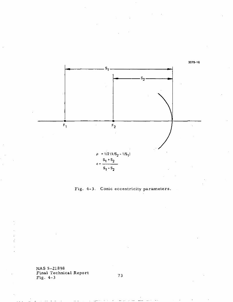
3079-16
p =1/2(1/S2- 1/S,)
e =S1+S2
S1-S2
Fig. 4-3. Conic eccentricity parameters.
NAS 5-21898Final Technical ReportFig. 4-3 73

and the eccentricity is
Sl + S2cJ s^ (4-19)Sl ' S2
Eccentricities for some typical surfaces are
Surface _«_ _K_
Sphere 0. 1.
Paraboloid 1. 0.
Ellipse 0 < € < i. 0 < K < 1
Hyperboloid € >1. K < Q.
The sagitta expression for a sphere would be
P Q 2
S° S r (4-17a)
soSO
and for a paraboloid
2P Q
s° (4-17b)
a. Ray Trace Equations — Denoting surface "s" with the
"s" subscript and the preceding surface by the "s-1" subscript.
Surface-to-surface transfer equations are
X = X , + -^il /t - Z . + Z ) (4-20)s s-1 n , \ s-1 s-1 s/ v
s- 1
m , , .Y = Y . + S (t . - Z . + Z (4-21)
s s-1 n , \ s-1 s-1 s/ x
74
Refraction at surface "s" converts optical direction cosinesl s- l> ms-l' and n s _! into la> mg, ng.
l
or
andi t
p = the inverse of the subnormal
ms = ms-l + P s s K - l ' V <4'23)
II
X ni S S
m = m - p Y n (4-23a)s so s s s v '
where
2 = £ , + P X n . (4-24)so s-1 s s s-1
m = m , + p Y n , (4-25)so s-1 s s s-1 v
P " = 7i 7n = - 7 - PS? ? \ i y ? + 4^ Q 2 + 6 p Q4 + 8Y Q6
s U d U 1 / K P ^ O V s s s s s ss so w
(4-26)
For the general asphere the appropriate values of Z and nS S
are found by iteration. Dropping the "s" subscript temporarily and
75
substituting i and i + 1 to indicate successive iterated values, the
iterations on Z and n are
r Z. p." (H . X. + m , Y.)b. _ 11 s-1 i s-1 in .
Zi + 1 = pT1!! i X. + m m (4-27)x s-1 i s- 1 in
s- 1
H 2 + n.2 - i2 - m.2 - 2 p " n. (£. X + m. Y )S 1 1 1 rS 1 1 S 1 S
2 fn. - p " (X 2. + Y m.)lLI r s s i s i - l
(4-28)
, 2 - f 2 - m 2 + n . 2 ( l + p » Q 2 )KS so so i \ Hs s / .. .
[ / »'? ? \ II 1 V*~t-7in. ( 1 + p Q - p (!> X + m Y )
1\ ^S S / ^S l SO S SO S'J
using starting values of Z. = 0 and n. = p. .
b. Spherical Surfaces — Though the above algorithms include
spherical surfaces as a special case, the tracing through spherical
surfaces is handled separately to expedite computing time. The trans-
fer equations are
X = X + H S> , (4-30)s so s s-1 v
Y = Y + H m . (4-31)s so s s-1
76
Z = H n ,s s s-1 (4-32)
X = Xso s- + JLadL(t T-z \n , \ s-1 s-1/s- 1
(4-33)
Y = Y ,so s-1
m 1 ,+ -^li ft ,-z .-n , \ s- 1 s-1/s- 1
(4-34)
The refraction equations are
2 = I . - P p Xs s-1 s ^s s
m = m . - P p Ys s-1 s "s s
n = n , - P / p Z - 1 )s s-1 s \ s s /
(4-35)
(4-36)
(4-37)
where H and P are determined as follows:s s
/ 2 2 v(A) = p X + Y )v ' Hs \ so so/ (4-38)
(B) = n , -v ' s-1I . + Y m .)
so s-1 so s-1/ (4-39)
ls = C5L2 . (4-40)
H = (A)s (B) + fjL cos i
S ** ••• S
(4-41)
77
p. cos r ='s s
Ls- l COS
(4-42)
ps = cos i (4-43)
These algorithms are listed here in the form they are used in the com-
putation which is necessary to preserve proper sign conditions.
c. Special Surface Forms — Some surface forms which can
be accommodated are noted below; most of them can be combined.
Cylinders
Toroids
Normal surfaces with cylindrical error
Periodic surface forms
These surface forms, mentioned above, are described by the
summation
(4-44)
?>1 is the expression for a cylindrical surface of curvature p, whose
axis may be rotated through an angle (p, Fig. 4-4. £,_ can combine
with £, to generate a toroidal surface where the surface (curve) gen-
erated by £- is rotated such that its vertex describes an arc of radius
l / p o - The arcs of p, and p2 lie in orthogonal planes. In Fig. 4-5(a)
it can be seen that the cylinder is generated by p.. when (p = p_ = 0.
Figure 4-5(b) is the cylinder generated by p_ when p, = (f> = 0. The
surface (curve or arc) C, may be the cross section of a sphere, any
conic or higher order surface form.
The periodic surface errors £ may be a radially symmetrical
sinusoidal (cosine in this case) variation of sagitta, a radial sine func-
tion or a combination of the two. These radial periodic errors may be
78
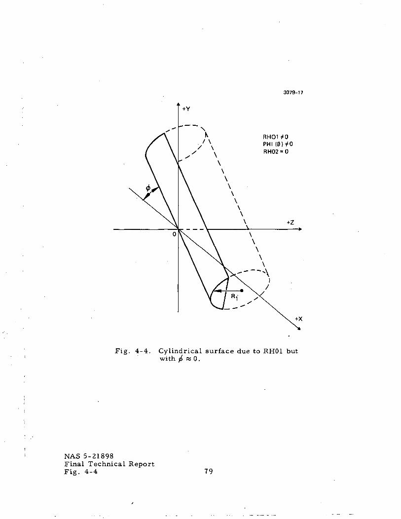
3079-17
+Y
RH01*0PHI (0 )^0RH02 = 0
Fig. 4-4. Cylindrical surface due to RH01 butwith ^ w 0.
NAS 5-21898Final Technical ReportFig. 4-4 79
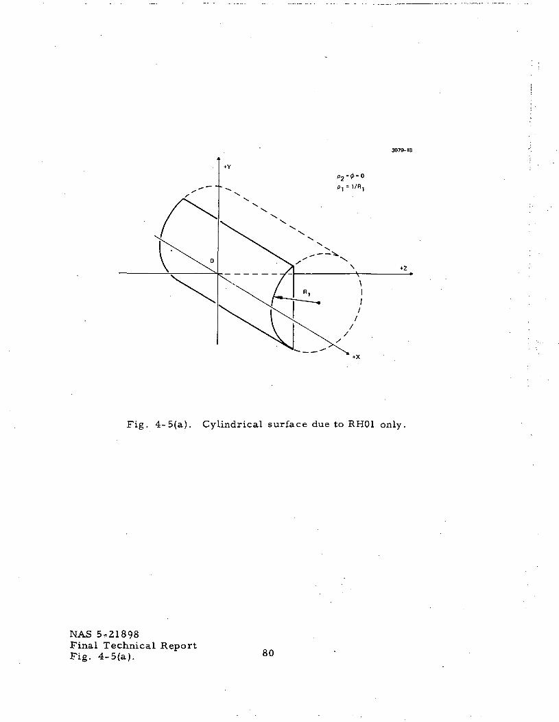
3079-18
Fig. 4-5(a). Cylindrical surface due to RH01 only.
NAS 5^21898Final Technical ReportFig. 4-5(a). 80
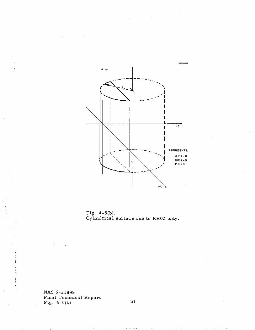
Fig. 4-5(b).CyLindrical surface due to RH02 only.
NAS 5-21898Final Technical ReportFig. 4-5(b) 81
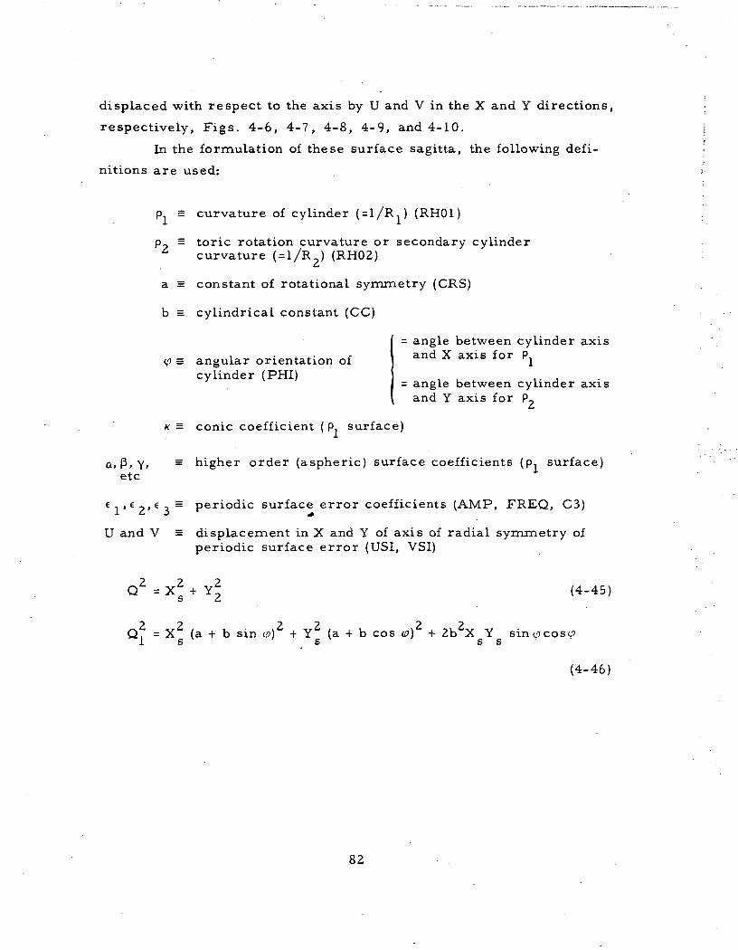
displaced with respect to the axis by U and V in the X and Y directions,
respectively, Figs. 4-6, 4-7, 4-8, 4-9, and 4-10.
In the formulation of these surface sagitta, the following defi-
nitions are used:
p = curvature of cylinder ( = 1/RJ (RH01)
p? = toric rotation curvature or secondary cylinder^ curvature ( = 1 / R ) (RH02)
a = constant of rotational symmetry (CRS)
b = cylindrical constant (CC)
= angular orientation of
= angle between cylinder axisand X axis for P
1cylinder (PHI) , u ,. ,
= angle between cylinder axisand Y axis for P_
K = conic coefficient (p. surface)
0 ,P ,v , = higher order (aspheric) surface coefficients (p, surface)etc
€ . , £ _ , € , = periodic surface error coefficients (AMP, FREQ, C3)
U and V = displacement in X and Y of axis of radial symmetry ofperiodic surface error (USI, VSI)
Q2 = xj + Y2 (4-45)
Q2 = X2 (a + b sin is)2 + Y2 (a + b cos cp)2 + 2b2X Y sinvcostfI S S S S
(4-46)
82
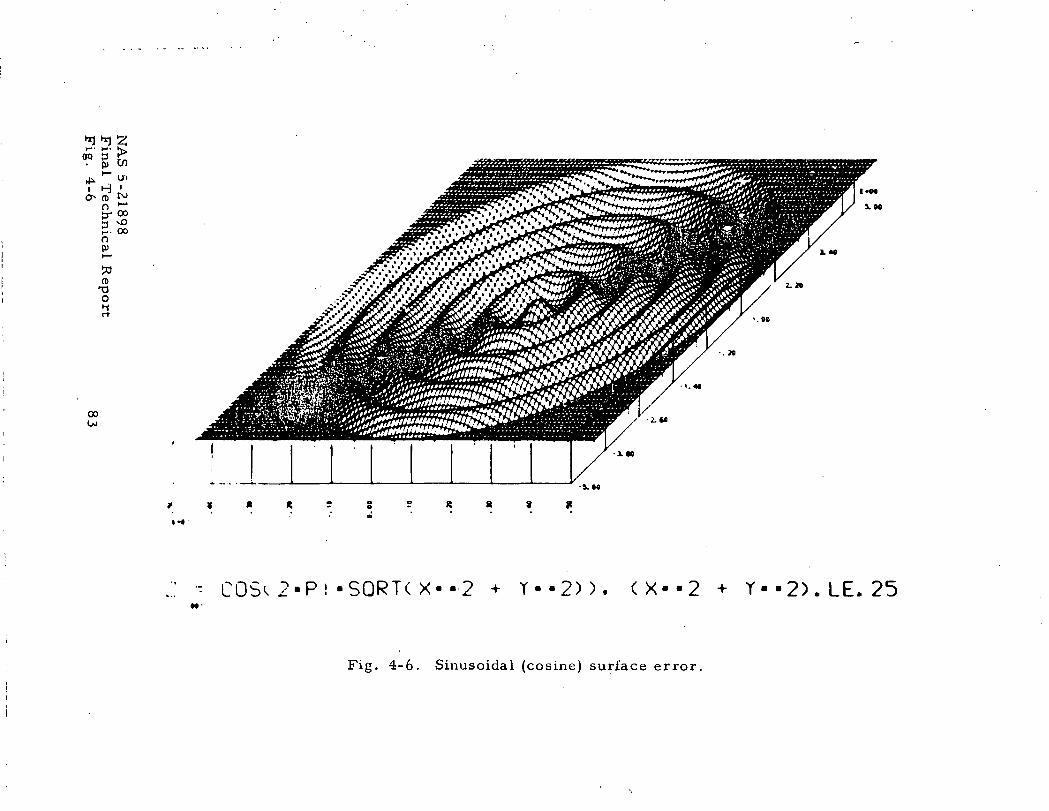
f nON 01
3 ^>Z. oon
13OH
00Oo
* *R *
COSk 2 - P ! - S Q R T C X - - 2 • » • Y - - 2 ) ) . ( X - - 2 • » • Y - - 2 ) . L E . 2 5
Fig. 4-6. Sinusoidal (cosine) surface error.
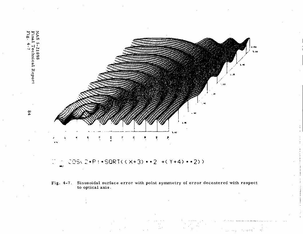
.
-Ij n> txj
&«5 ^oM- 00n
JO' (D
00
i-cevoo
OSv 2-P ! - S Q R T C C 2 +( Y + 4) • - 2 > >
Fig. 4-7. Sinusoidal surface error with point symmetry of error decentered with respectto optical axis.
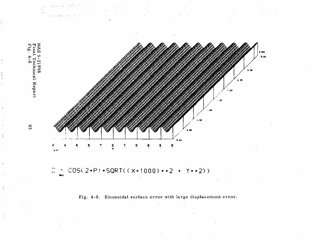
OQ 0• p) CO
,jx *" Ul
oo n> ^s-s2.»op>
(B•T3o
ooen
V 00
8 Jt
COSC 2 -P! -SQRTC ( X + 1 0 0 0 ) • -2 -«• Y - - 2 ) )
Fig. 4-8. Sinusoidal surface error with large displacement error.

OP 3
f
.. oo
(D'rao
00
C X - - 2
Fig. 4-9- Sine function surface error.
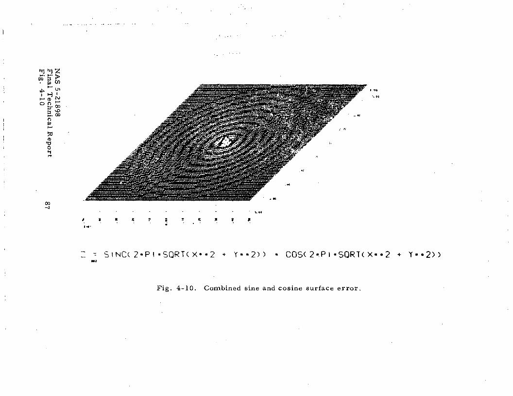
TO' 5' >. pj Cfl
sog. oo
o>T3O
00-J
* * * R *
'• S INCC 2-P l -SQRTC X- -2 + Y - - 2 ) ) - COS( 2-P I - S Q R T C X-• 2 + Y - - 2 ) )
Fig. 4-10. Combined sine and cosine surface error.
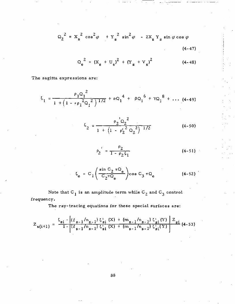
0 = X cos <f> + Y sin <p - 2X Y sin w cos2 s ^ s ^ s s ^
(4-47)
Qe2 = (Xg + Us)
2 + (Yg + Vg)2 (4-48)
The sagitta expressions are:
•1 - , , /, ... 2^TTT72 + *Q14 + PQ16 + YQ18 + •'• (4-49)20| 1 - Kp1 Uj
P / Q 2 .7T (4-50)
i P
"2 =T^T7- (4-5D
sin C? irQ \C.Q e ) c o s C 3 . Q e (4-52)
Note that C, is an amplitude term while C,, and C_ control
frequency.
The ray- tracing equations for these special surfaces are:
Zsi
88
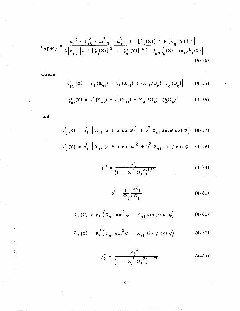
n
- n - n .s s 0 s 0 sis(i+D
2 i
(Y)]
(4-54)
where
. (4-56)
and
2 . , 2,. (X) = p, X . (a + b sin <p) + b Y . sin (p cos <p \ (4-57)l J . L S I s i J
' (Y) = p'' [Y . (a + b cos (/?)2 + b2 X . sin(/?cos(p| (4-58)1 X I S I S I J
IIpl = PIl/2 (4-59)
(4-60)
' (X) = p'' (x . cos2 (O - Y . sin </> cos <p\ (4-61)Z i \ si ^ si T V
= P2 (Ysi Sin . sin cos (4-62)
2 ^ 2\ 1/2(4-63)
89
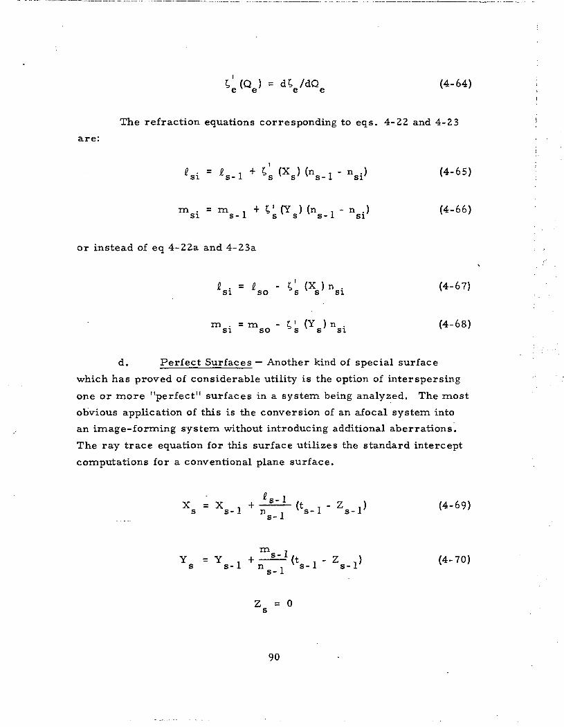
r, (Q ) = d; /dCJ (4-64)6 6 6 6
The refraction equations corresponding to eqs. 4-22 and 4-23
are:
m . = m . + V (Y ) (n . - n .) (4-66)si s-1 s v s ' * s-1 si v '
or instead of eq 4-22a and 4-23a
& . - I - ?,' (X ) n . (4-67)si so s v s si v '
m . = m - C' (Y ) n . (4-68)si so 's s si l
d. Perfect Surfaces — Another kind of special surface
which has proved of considerable utility is the option of interspersing
one or more "perfect" surfaces in a system being analyzed. The most
obvious application of this is the conversion of an afocal system into
an image-forming system without introducing additional aberrations.
The ray trace equation for this surface utilizes the standard intercept
computations for a conventional plane surface.
Xs = Xs-l +ls- 1
m ,Y = Y . +—^-(t , - Z .) (4-70)
s s-1 n i s-1 s-1 x
s- 1
Z = 0s
90
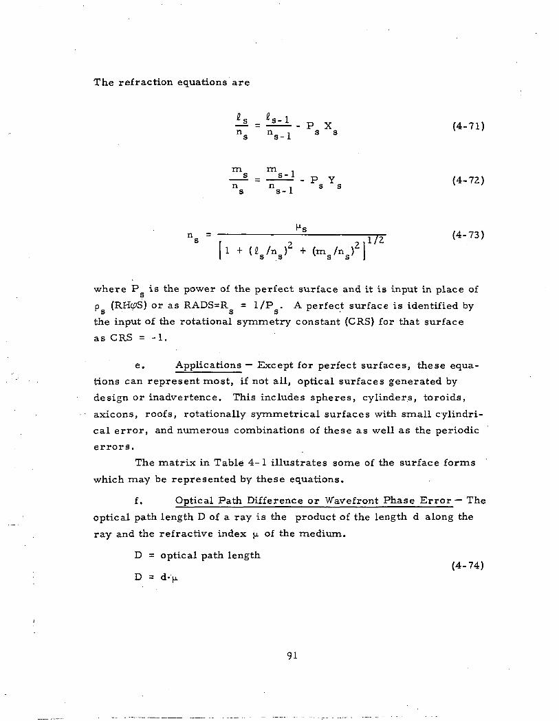
The refraction equations are
«8 Vl- Pa X. (4-71)
ns ns-l s s
m in ,= —— - P Y (4-72)
n n .. s ss s-1
[l -MVV2 + ( m s / n g ) 2 j
(4.73)
where P is the power of the perfect surface and it is input in place ofS
p (RH<pS) or as RADS=R = 1/P . A perfect surface is identified byS S S
the input of the rotational symmetry constant (CRS) for that surface
as CRS = -1.
e. Applications — Except for perfect surfaces, these equa-
tions can represent most, if not all, optical surfaces generated by
design or inadvertence. This includes spheres, cylinders, toroids,
axicons, roofs, rotationally symmetrical surfaces with small cylindri-
cal error, and numerous combinations of these as well as the periodic
errors.
The matrix in Table 4-1 illustrates some of the surface forms
which may be represented by these equations.
f. Optical Path Difference or Wavefront Phase Er ror— The
optical path length D of a ray is the product of the length d along the
ray and the refractive index ^ of the medium.
D = optical path length(4-74)
D = d-(jL
91
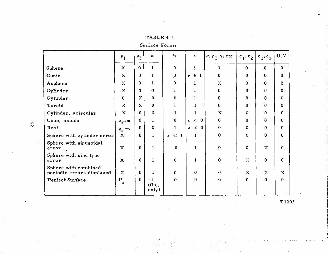
TABLE 4-1
Surface Forms
Sphere
Conic
Asphere
Cylinder
Cylinder
Toroid
Cylinder, acircular
Cone, axicon
Roof
Sphere with cylinder error
Sphere with sinusoidalerror
Sphere with sine typeerror
Sphere with combinedperiodic errors displaced
Perfect Surface
Pl
X
X
X
X
0
X
X
Pg-CO
ps— «X
X
X
X
ps
P2
0
0
0
0
X
X
0
0
0
0
0
0
0
0
a
1
1
1
0
0
0
0
1
0
1
1
1
1
-1(flagonly)
b
0
0
0
1
0
1
1
0
1
b « 1
0
0
0
0
K
1
K ± 1
1
1
1
1
1
K < 0
K < 0
1
"
1
1
0
0
a, P r Y, etc
0
0
X
0
0
0
X
0
0
0
0
0
0
0
C1'C2
0
0
0
0
0
0
0
0
0
0
0
X
X
0
C1'C3
0
0
0
0
0
0
0
0
0
0
X
0
X
0
u,v
0
0
0
0
0
0
0
0
0
0
0
0
X
0
\Dtv
T1203
Defining the optical path length for a ray passing from surface s-1 to
surface s to be D , it can be shown thats
_ ( t s - l - Zs-l + Zs} 2 (4-75)ns-l H"1
The total path length through the complete system is the sum
of all the surface-to-surface values and is defined to be D*.
n
D* = D + D (4-76)s- 1
which is in practice the summation from entrance pupil to exit pupil.
D is the distance along the ray from the object point to the entranceo -1
pupil for a finite object, i.e. L ^ 0.
0) (4-77)
For infinite conjugates, D is the distance from the incident plane wave
to the entrance pupil.
D = m y (L "-1 = 0) (4-78)o o o o
where
y E entrance pupil ray intercept.
Note that for the infinite conjugate axial case m = 0., hence
D = 0. The difference between the total optical path length D* for
an arbitrary ray and that D* for a reference ray is the optical path
difference or wavefront departure W for the given ray.
93
W = D* - D* . (4-79)
W can be expressed as the sum of a set of W's at each
surface
N N
>T
W = D + \ D - D - \ Do /, s co /, cs
= D - D + \ (D - D )O CO S CS
N
IN
0
or, defining
(Dg - Dcs) (4-80)
W = D - D . (4-81)s s cs v '
Then, for the ray corresponding to exit pupil coordinates (u, v)
the overall optical path difference for that ray is W(u, v) and
N
W(u,v) = W . (4-80a)s = 0 s
Denoting the ray parameters for the arbitrary ray with the
subscript s and those for the reference ray with the subscript cs and
substituting (4-75) into (4-81),
2H-- i [
W = Z—i n . (Z - Z ,) -n ,(Z -Z ,)s n , n , I cs-1 x s s-1 s-1 cs cs-1
+ ts-l *ncs-l " ns- l ) l (4-82)
94
Generalizing (4-82) to allow treatment of tilted and/or decentered
surfaces
2
W = W -- — - In' . (Z - Z *) -n' . (Z - Z *) ]s so ' ' I cs-1 v s s ' s-1 v cs cs '
(4-83)
ns-lncs-l
where
2
Wso
[i 1 r= - — - (n , -n . ) t , -n . Z Z + n , Z I
n , n , lv cs-1 s-1 s-1 cs-1 cs-1 s-1 s-1 cs-1s- 1 cs- 1 J
(4-84)
The primed and starred quantities of equation (4-83) are defined
in Section 4.6 on tilt and decentration. W represents the path dif-S O
ference from surface "s-1" to the nominal tangent plane of surface "s".
The remainder of eq. (4-83) represents the path difference from the
nominal, untilted tangent plane of surface "s" to the tilted and/or
decentered surface itself.
g. Perfect Surface OPD — When using the perfect surface
option, the optical path difference for the surface is computed as
follows:
W = W - Ps so
2\ / 2 2 \+ Y ^ . n (X + Y ) . ns / s \ cs cs/ csu. + n u + n
s s s cs
(4-85)
95
4.4 VIGNETTING AND OBSCURATION
a. Vignetting — Vignetting must be accommodated and
L.ACOMA handles it in two ways; at the entrance pupil or on a surf ace-
by-surf ace basis.
If the nature of the vignetting at the entrance pupil is known,
this vignetting may be described by the input of a value V_ = VZERO
or VTT = VPI representing the fractional vignetting, respectively, in
the upper or lower portion of the entrance pupil. A different set
(V_, V^) must be input for each field fraction K. The interpretation of
the magnitude of the input value of V is as follows:
V = 0 or 1. 0 no vignetting
0 < V < 1. 0 normal vignetting
The other means for handling vignetting can replace or augment
the pupil vignetting. This is accomplished by the input of clear aperture
data for each surface. As each ray is traced through the surface, a test
determines whether the ray falls outside the clear dimensions in which
case it is terminated.
b. Obscuration — As with vignetting, there are two
approaches to obscuration, either in the entrance pupil or on a surf ace-
by-surface basis. At the entrance pupil, the descriptive data are:
UZERO for the radius of the obscuration; GZERO representing the
distance from the center of the entrance pupil to the upper edge of the
obscuration; and GPI, the distance from the center of the entrance
pupil to the lower edge of the obscuration. A set (UZERO, GZERO,
GPI) is required for each field angle to be traced. A circular centered
obscuration would have•
GZERO = UZERO = - GPI
Other cases can of course be accommodated.
96
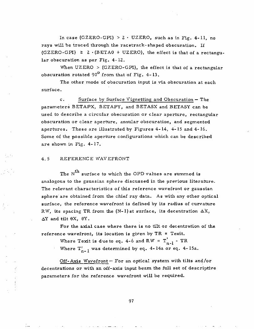
In case (GZERO-GPI) > 2 • UZERO, such as in Fig. 4-11, no
rays will be traced through the racetrack-shaped obscuration. If
(GZERO-GPI) £ 2 -(BETAO + UZERO), the effect is that of a rectangu-
lar obscuration as per Fig. 4-12.
When UZERO > (GZERO-GPI), the effect is that of a rectangular
obscuration rotated 90° from that of Fig. 4-13.
The other mode of obscuration input is via obscuration at each
surface.
c. Surface by Surface Vignetting and Obscuration — The
parameters BETAPX, BETAPY, and BETASX and BETASY can be
used to describe a circular obscuration or clear aperture, rectangular
obscuration or clear aperture, annular obscuration, and segmented
apertures. These are illustrated by Figures 4-14, 4-15 and 4-16.
Some of the possible aperture configurations which can be described
are shown in Fig. 4-17.
4.5 REFERENCE WAVEFRONT
f~TiThe N surface to which the OPD values are summed is
analogous to the gaussian sphere discussed in the previous literature.
The relevant characteristics of this reference wavefront or gaussian
sphere are obtained from the chief ray data. As with any other optical
surface, the reference wavefront is defined by its radius of curvature
RW, its spacing TR from the (N-l)st surface, its decentration AX,
AY and tilt 6X, 6Y.
For the axial case where there is no tilt or decentration of the
reference wavefront, its location is given by TR = Texit.
Where Texit is due to eq. 4-6 and RW = l' ^ - TR
Where T1 , was determined by eq. 4-14a or eq. 4-15a.
Off-Axis Wavefront— For an optical system with tilts and/or
decentrations or with an off-axis input beam the full set of descriptive
parameters for the reference wavefront will be required.
97
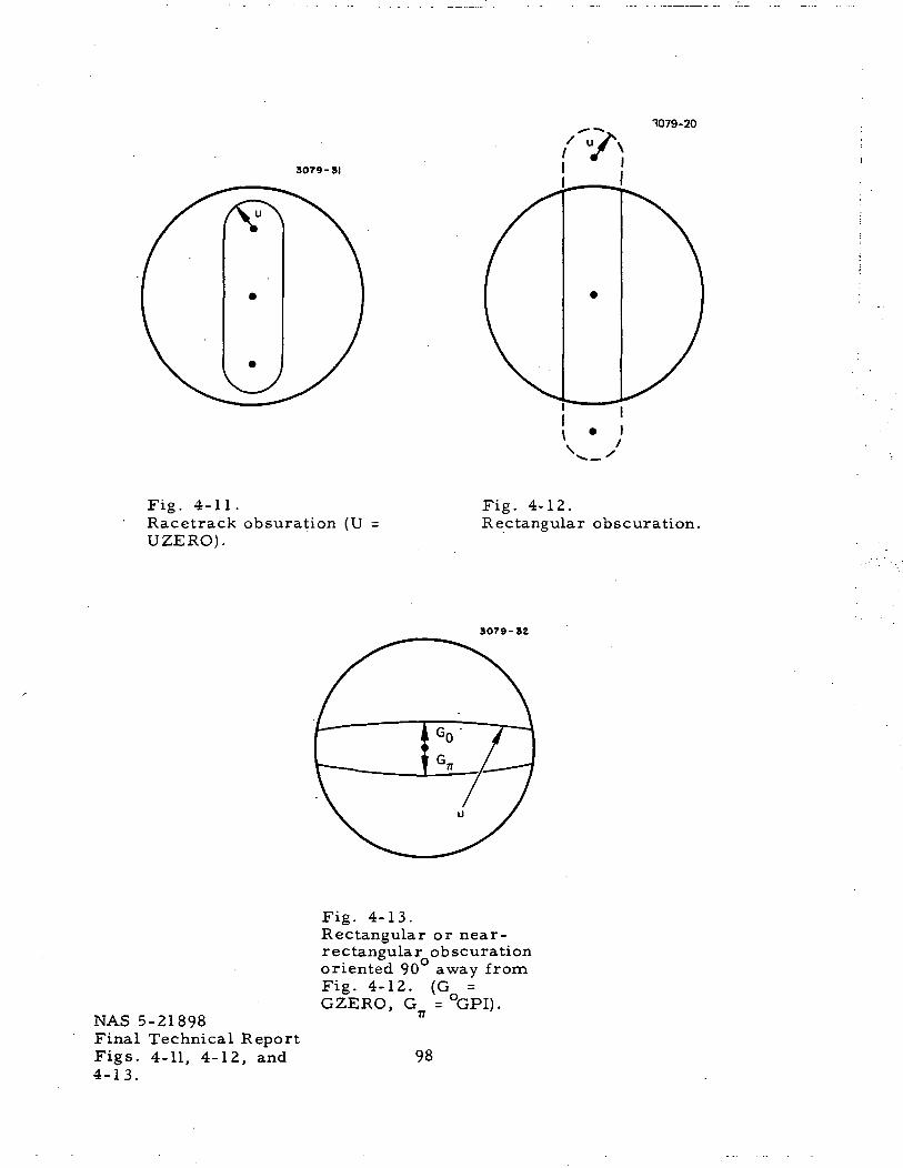
1079-20
3079-SI
Fig. 4-11.Racetrack obsuration (UUZERO).
Fig. 4-12.Rectangular obscuration.
3079-32
NAS 5-21898Final Technical ReportFigs. 4-11, 4-12, and4-13.
Fig. 4-13.Rectangular or near-rectangular obscurationoriented 90 away fromFig. 4-12. (G =GZERO, G = °GPI).
77
98
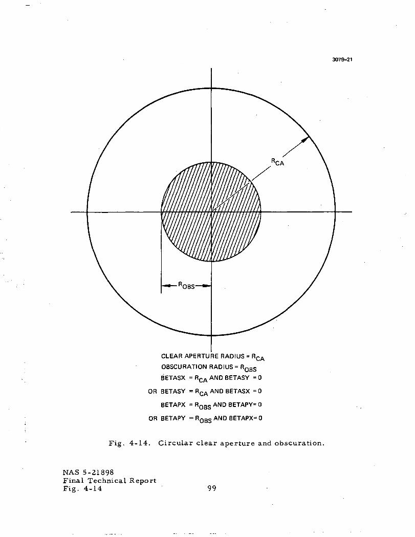
3079-21
CLEAR APERTURE RADIUS = RQA
OBSCURATION RADIUS = ROBS
BETASX = RCA AND BETASY = 0
OR BETASY = RCA AND BETASX =0
BETAPX = RQBS AND BETAPY= 0
OR BETAPY = RQBS AND BETAPX= 0
Fig. 4-14. Circular clear aperture and obscuration.
NAS 5-21898Final Technical ReportFig. 4-14 99
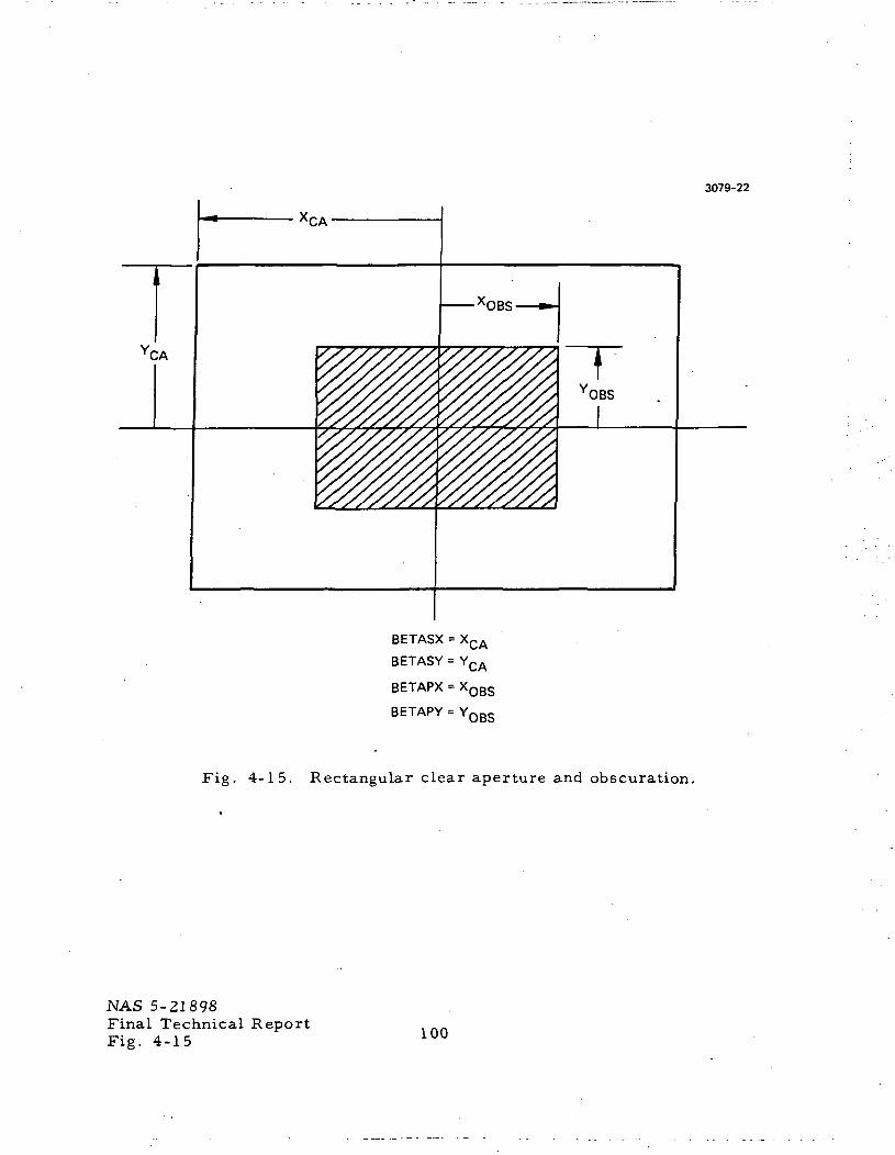
3079-22
rCA
'•DBS-
'OBS
BETASX = XCA
BETASY = YCA
BETAPX = XQBS
BETAPY = YQBS
Fig. 4-15. Rectangular clear aperture and obscuration.
NAS 5-21898Final Technical ReportFig. 4-15 100
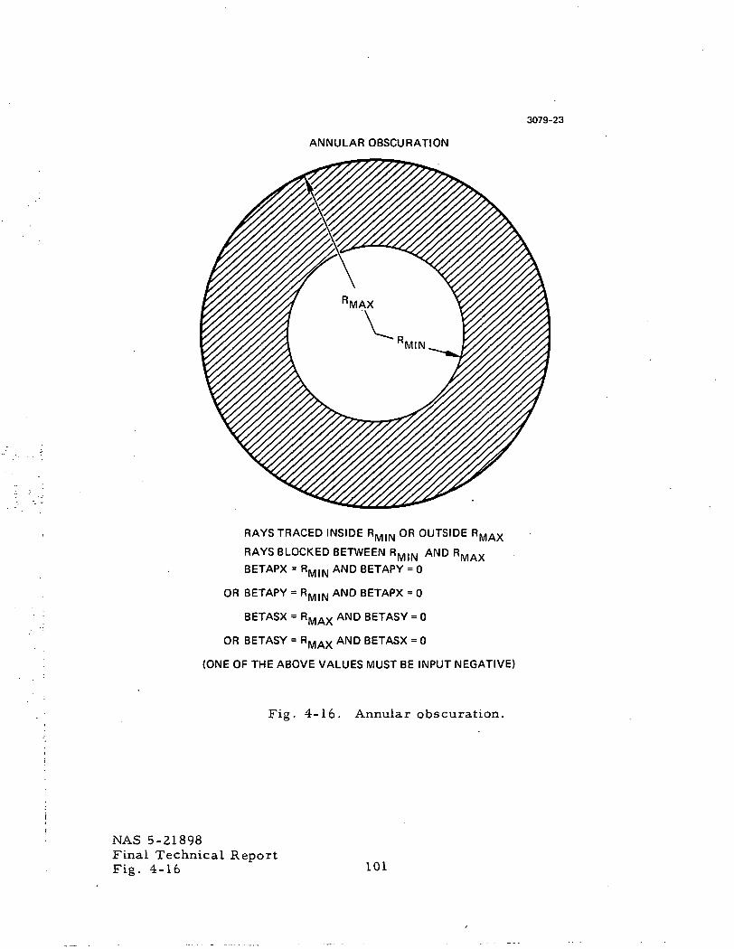
3079-23
ANNULAR OBSCURATION
RAYS TRACED INSIDE RM)N OR OUTSIDE RMAX
RAYS BLOCKED BETWEEN RM|N AND RMAX
BETAPX = RM,N AND BETAPY = 0
OR BETAPY = RM|N AND BETAPX = 0
BETASX = RMAX AND BETASY = 0
OR BETASY = RMAX AND BETASX = 0
(ONE OF THE ABOVE VALUES MUST BE INPUT NEGATIVE)
Fig. 4-16. Annular obscuration.
NAS 5-21898Final Technical ReportFig. 4-16 101
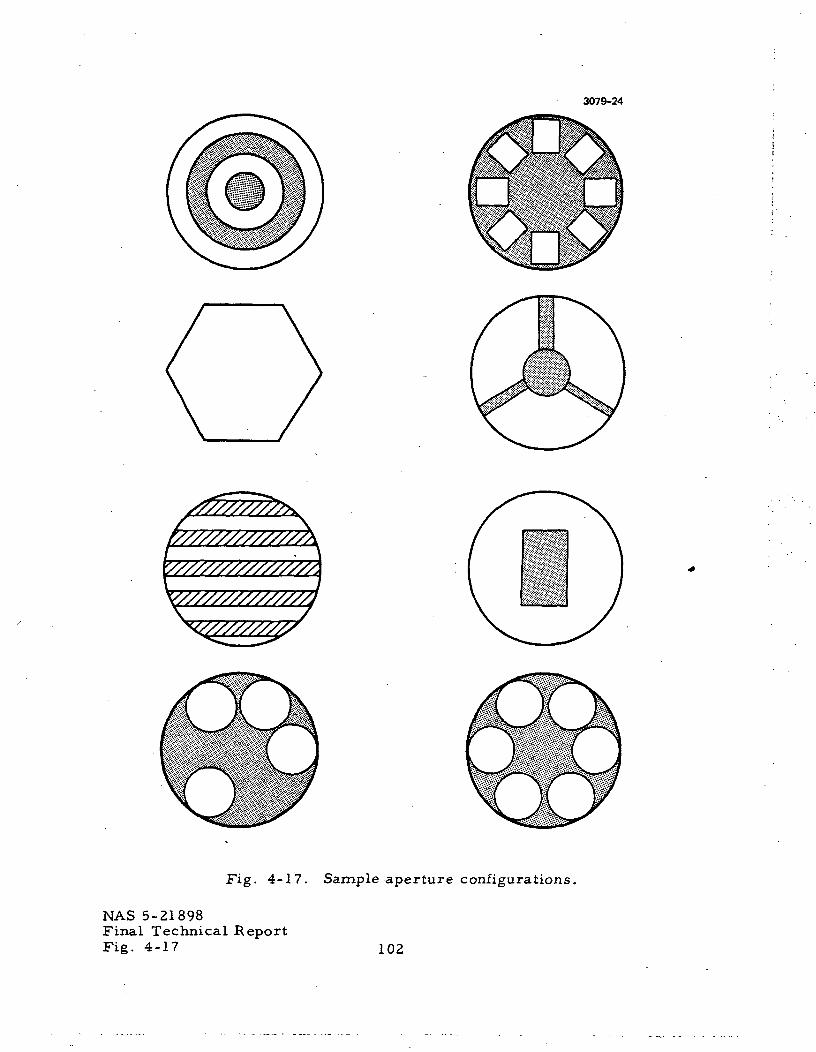
3079-24
Fig. 4-17. Sample aperture configurations.
NAS 5-21898Final Technical ReportFig. 4-17 102
RW is the distance along the chief ray from its intersection or
point of closest approach to the optical axis (exit pupil position) to its
point of intersection with the image surface. The angular components
of the chief ray give the tilt of the reference wavefront, etc. The com-
putation of RW, T , 6X, 6Y, AX and AY is as follows.
Given i , m , n , for the chief ray exiting the optical train and
the chief ray intercepts X , Y and Z at the focal surface, if m 4 0c c c c
Y v- iRW = c
mn" i (4-86)c
Y nTR = T ' , —- + Z (4-87)n- 1 m c ^
s. y= X —- (4-88)c m v 'c
AY = 0.
If m =0 and i 4 0c c
X ^ ic n"A (4-89)c
X nTR = T' —- + Z (4-90)
AX = 0.
m RWAY = Y . (4-91)
c v- irs- 1
103
The reference wavefront tilt angles are
6X = ARCTAN (I /n ) (4-92)
6Y = ARCTANm
c
nc
(4-93)
For a case with an IMC so that the reference wavefront is off-
axis but X —• Y —- 0, TR is defined as that for the axial case and
(T' - TR)Hj,,! (4-94)
I RWAX = X - _j= (4-95)
C K
m RWAY = Y - — . (4-96)
Equations 6X and 6Y are defined per eqs. 4-92 and 4-93.
4.6 TILT AND DECENTRATION
The tilt and decentration procedure utilizes conventional
coordinate transformation matrices.
The procedure is to trace a ray to the tangent plane for the cen-
tered surface and then locate the intersection point of the ray with the
tilted-dec entered tangent plane, transform the optical direction cosines
of the ray into the rotated coordinate system, and then trace the ray
from the new tangent plane to the surface.
104
The transformation matrix represents the relocation of the
origin by AX, AY and AZ followed by rotation of this displaced coordi-
nate system. The rotation begins with a 6Z around the optical axis fol-
lowed by the rotation 6Y around the X' axis where the X1 indicates the
new X axis due to the Z rotation. 6X is the rotation about the Y1 axis
which is the result of the BZ, 8Y rotations.
Representing the new optical direction cosines with primes,
£' = g . (cos 9X cos 6Z + sin ex sin 6Y sin 6Z)S — -I S ~ J-
-m , cos 6Y sin 6Z + n .s-1 s- 1
(cos 6X sin 6Y sin 6Z - sin 6X cos 6Z) (4-97)
m ' , = m , cos 6Y cos 6Z - n , (sin 6X sin 6Z -f cos 6X sin 6Y cos 6Z)s-1 s-1 s-1
+ I . (cos 6X sin 6Z - sin 6X sin 6Y cos 6Z) (4-98)s- 1
n' , = n , cos 6X cos 6Y + g . sin 6X cos 6Y + m , sin 6Y .s-1 s-1 s-1 s-i
(4-99)
The values X*, Y* and Z* represent the intercept coordinates
of the ray with the nominal tangent plane expressed in the transformed
coordinate system relative to the new tangent plane.
X* = (XSO-AX) (cos 6X cos 6Z + sin 6X sin 6Y sin 6Z)
-(YSO-AY) • cos 6Y sin 6Z - AZ
(cos 6X sin 6Y sin 6Z - sin 6X cos 6Z) (4-100)
105
Y* = (YSO-AY) cos 6Y cos 8Z + AZ (sin 6X sin 6Z + cos 6X sin 6Y cos 6Z)
+ (XSO-AX) (cos 6X sin 6Z = sin 6X sin 6Y cos 6Z) (4-101)
Z* = (XSO-AX) sin 6X cos 6Y + CYSO-AY) sin 6Y - AZ cos 6X cos 6Y .
(4-102)
Thus X' and Y' represent the intersection of the ray with the newSO SO
tangent plane and
Xso = X * - ~ - Z* (4-103)
m' .r = Y* — Z* (4-104)SO ni is- 1
Zso =
a. Sign Convention — The origin (surface vertex) of the trans-
formed coordinate system has the coordinates AX, AY, AZ relative to
the original origin (Fig. 4-18). Viewed along the positive direction of
the optical axis, +6Z represents a counterclockwise rotation about the
optical (Z) axis. Similarly, a tilted surface has its optical axis oriented
at the angles 6X and 6Y with respect to the axis of the preceding optical
surface. A surface tilted by +6Y (or + 6X) has it axis rotated such that
its new direction relative to the original axis is the same as would a
ray having positive direction cosines m and n. For example, a ray
parallel to the original axis (j0 = m = 0, n= 1), and incident upon a
surface tilted by a positive 6Y will have transformed incident direction
cosines so that m < 0 (see Fig. 4-19).
106
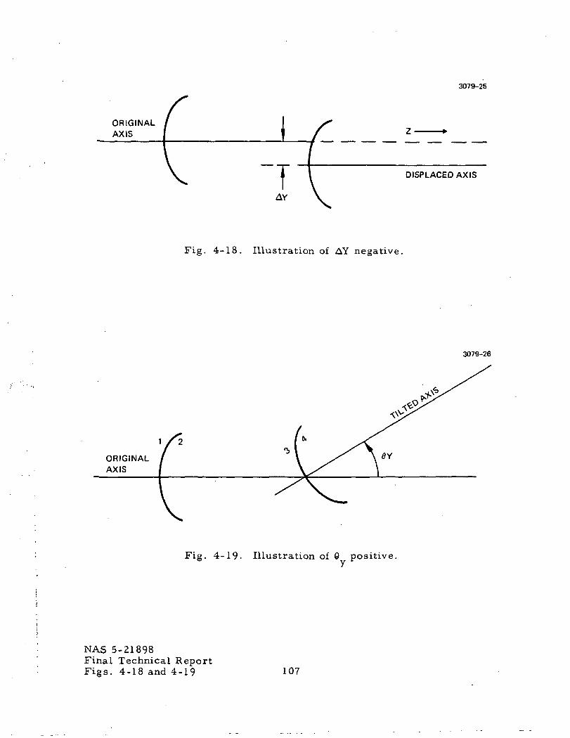
3079-25
ORIGINALAXIS
TAY
DISPLACED AXIS
Fig. 4-18. Illustration of AY negative.
Fig. 4-19- Illustration of 0 positive.
3079-26
NAS 5-21898Final Technical ReportFigs. 4-18 and 4-19 107
b. Coordinate Restoration — If a surface is tilted or
decentered, all the surfaces following will be aligned with the tilted or
decentered surface. Therefore, the tilt or decentration of a single
surface amounts to tilting or dec enter ing the system following the tilt
with respect to the portion of the system preceding the tilt. If it is
desired to misalign a given surface in the midst of a centered optical
system, it is necessary to introduce a reverse tilt or decentration
immediately following the misaligned surface to restore the coordinate
system. If there is a combination of AX, AY, AZ and/or 6X, 6Y, 6Z
at the surface, then because of the sequence of the operation of the
decentrations and tilts the combination of -AX, -AY, - 6X, -6Y, etc.
will not necessarily restore the proper coordinates. The following
are rules to follow in the restoration of the coordinate system after
traversing a misaligned surface:
1. Restoration after a single tilt 6Y or a singledecentration AX is accomplished with the inser-tion of a dummy surface following the misalignedsurface with p = 0, Tg_ ^ = 0 and the refractiveindex (J-s the same as that following the misalignedsurface. The dummy plane should have a tilt of-6Y or a decentration of -AX.
«2. For a surface having tilts 6X, 0Y, 6Z and decen-
trations AX, AY, AZ. Four dummy planes mustbe inserted:
Dummy plane No. 1 with -6XDummy plane No. 2 with -6YDummy plane No. 3 with -6ZDummy plane No. 4 with -AX, -AY, -AZ
3. For surfaces with more than one but less than thefull six misalignment components the sequence ofthe operations must remain the same removingdummy planes which do not apply. For a surfacewith 6X, 6Z and AY three dummy planes are used:
Dummy plane No. 1 with - 0XDummy plane No. 2 with - 6ZDummy plane No. 3 with -AY
108
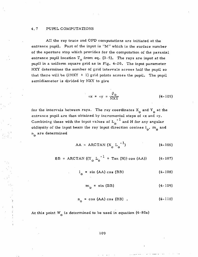
4.7 PUPIL, COMPUTATIONS
All the ray trace and OPD computations are initiated at the
entrance pupil. Part of the input is "M" which is the surface number
of the aperture stop which provides for the computation of the paraxial
entrance pupil location T from eq. (3-5). The rays are input at the
pupil in a uniform square grid as in Fig. 4-20. The input parameter
NXY determines the number of grid intervals across half the pupil so
that there will be (2NXY + 1) grid points across the pupil. The pupil
semidiameter is divided by NXY to give
- = < y = *FxV <4-105>
for the intervals between rays. The ray coordinates X and Y at the
entrance pupil are then obtained by incremental steps of ex and ey.
Combining these with the input values of L and H for any angular
obliquity of the input beam the ray input direction cosines 1 , m and
n are determinedo
AA = ARCTAN (X L ~l) (4-106)
BB = ARCTAN ((Y L " l -I- Tan (H)) cos (AA)) (4-107)
1 = sin (AA) cos (BB) (4-108)
mQ = sin (BB) (4-109)
n = cos (AA) cos (BB) . (4-110)
At this point W is determined to be used in equation (4-80a)
109
3079-27
Fig. 4-20. Uniform square ray grid.
NAS 5-21898Final Technical ReportFig. 4-20 110
For L ~ = 0o
For L "1 4 0o
(4-111)
w = J, Io n cos (H) (4-112)
Pupil Amplitude Values (B(u, v)) — The pupil coordinates are
here referred to as u, v which coincides with the notation used in dis-
cussing computation of the amplitude spread function (Section 4. 8) u
and v apply to the exit pupil coordinates while X and Y represent the
entrance pupil coordinates for the given ray.
The entrance pupil amplitude values axe determined as follows:
Transmitter — Truncated gaussian amplitude distribution with
total radiant power per input parameter P .
Receiver — (Received signal)— Uniform amplitude distribution
if P0 is input positive it is the uniform intensity value I . If P is input
negative it is the total radiant power, then
Io = |PJ/A0 (4-113)
where
then
A = entrance pupil area
Receiver- Local Oscillator— Truncated gaussian amplitude dis-
tribution with total radiant power per input parameter P .
I l l
Truncated Gaussian Intensity Function— The pupil amplitude
function B(u, v) for a gaussian amplitude distribution is defined as
follows:
P = Total input beam power (W)
I = peak intensity of gaussian beam
w = 1 /e intensity radius
(3 = maximum input beam radius or truncation radius
2 2 , 2r = u + v
2PI = - 5 - ,- ? - =• (4-115)o 2 . -2 Pr/ /w 2 v 'r
o. - r /w(1 - e r° / 10
2 , 2r /Wo (4-116)
B(u,v.) = v / I (u ,v ) . (4-117)
The amplitude expressions, eq. (4-114) and (4-117), assume unit
magnification between entrance and exit pupils. If the pupil magnifica-
tion mP is not unity it will modify B(u, v).
., .c. .. TD entrance pupil diameter ,A 1 1 0»pupil magnification = mP = exit pupil Diameter (4-118)
B'(U,V) = mP • B(u,v) . (4-119)
4. 8 AMPLITUDE SPREAD FUNCTION
The complex impulse response function or amplitude spread
function ASF(x, y) at the Fraunhofer plane is the two dimensional Fourier
transform of the pupil function F(u, v).
112
rFor the received signal
ASFl(x,y) = FRl(x.y) + i FIl(x,y) (4-123)
PSFl(x,y) = |ASFl(x,y)|2 (4-124)
and for the local oscillator
ASF2(x,y) = FR2(x,y) + i FI2(x,y) (4- 123a)
PSF2(x,y) = |ASF2(x,y)|2 . (4- 124a)
Signal power, local oscillator power and heterodyne power are
obtained by numerical integration over the specified detector dimensions.
The computed ASF and PSF values are obtained for a uniform
grid of intervals AX, AY.
Signal Power = POWER(l) = Z 2PSF1 (x,y) AX AY (4-125)x y
L.O. Power = POWER (2) = LSPSF2 (x.y)AXAY . (4-126)x y
Heterodyne Power — If the nominal phase difference between the
receiver signal beam and the local oscillator beam is zero, heterodyne
power is obtained with J12 (x,y).
Heterodyne Power = POWER(3) = 2 ZJ12(x,y) AX AY (4-127)x y
where
J12(x,y) = FRl(x.y) FR2(x,y) + FIl(x,y) F12(x,y) (4-128)
113
ASF(x,y) = ff. F(u,v) (4-120)
^"denotes Fourier transform
F(u,v) = B(u,v) • exp [-1K • W(u, v)] (4-121)
K = 2ir /X .
With B(u,v) from (4-114) or (4-117) and (4-119) with W(u, v)
from (4-80a).
ASF(x,y) = ~^ f/F(u,v) • exp [^(ux + vy) dudv. (4-120a)
The complex amplitude function ASF(x, y) is represented by the
real function FR(x, y) and the imaginary function FI(x,y).
ASF(x, y) = FR(x,y) + i FI(x, y) . (4- 12 Ob)
The intensity function or point spread function is PSF(x.y)
PSF(x.y) = |ASF(x,y) | 2 (4-122)
= [FR(x,y) + i FI(x,y)] [FR(x, y) -iFI(x,y)] . (4- 122a)
The functions ASF(x, y) and PSF(x, y) provide the basis for the
quality criteria for the receiver and transmitter.
4.9 RECEIVER QUALITY CRITERIA
The amplitude spread function ASF(x, y) and point (intensity)
spread function PSF(x, y) are determined for the received signal beam
and the local oscillator (L.O. ) beam.
114
or for brevity,
J12 = FR1 FR2 + FI1 F12 . (4-128a)
If there is a. nominal phase difference (A<J>) between the two beams, that
phase component must be removed to obtain J12:
Heterodyne power = POWER(3) = 22 J121 (x, y) AX AYx y
(4-129)
J12' = FR1' FR2 + FIT F12 (4-130)
J12' = (FRI cos A4> - FI1 sin A<)>) FR2
+ (FI1 cos A<|> + FRI sin A4>) FI2
J121 = (FRI FR2 + FI1 FEZ) cos A$
+ (FI2 FRI - FI1 FR2) sin Acj>
J121 = J12 cos A4> + K12 sin Atf> (4-130a)
where
K12 = FI2 FRI - FI1 FR2 (4-131)
Phase minimization — The value of J121 will be maximized when
d(J12'/d(A<j>) = 0.
= J12 sin A* + K12 cos A6 (4-132)
with
d(J12')d
115
J12 sin A<J> = K12 cos A<J>
sin AA K12 ,2 - tan
The value of A<f> is then obtained by the summation over the
specified detector as follows
Tan = Z2K12 (X Y)x y
SSJ12 (X Y)x y x
(4-133)
The remaining received signal quality criteria are determined
as follows:
Phase Match Efficiency = (4- 134)
POWER (3) = Heterodyne power
POWER (5) =2Z [PSF1(X,Y) PSF2(X,Y)]1/2AXAYx y
(4-135)
Optical transmission = PZERQ (4-136)
POWER(6) = Exit pupil power
PZERO = Total received power
Focusing Efficiency = (4-137)
Nonheterodyne detection efficiency = — pzERQ (4-138)
T _ ... . .. „. . POWER(5)Li.O. illumination efficiency =•— •*•"* TTT
(POWER(l) POWER(2) '
116
4"TT AMaximum Antenna Gain = _ o (4- 140)
A = entrance pupil area
X. = spectral wavelength
Receiver efficiency to I. F. = ' <4' 141>
4. 10 TRANSMITTER QUALITY CRITERIA
The point (intensity) spread function PSF(X, Y) is determined for
the transmitter at the specified range. The quality criteria for the
transmitter are:
Peak intensity = IP = maximum value of PSF (X, Y) (4-142)
Optical transmission = Pp^^j6) (4-143)
Maximum antenna gain = 4TT PQWER(7? (4. 144)
*•
POWER(7) = Effective exit pupil area
X- = Spectral wavelength
IP (RW X)Overall transmitter efficiency = pzgRQ pQWER(7)' ^4
where RW = Range.
117
4.11 ERROR ANALYSES
The errors associated with these computations come from
numerous sources. The major error sources are discussed here with
some indication of guidelines to be followed to keep them to a minimum.
a. Aberrations — The conventional Fraunhofer diffraction
integrals used in these computations are derived based on certain
approximations. The fundamental integral involves the exponential
exp [iK(W + S)] (4-146)S
where W = OPD error for a given point on the wavefront and S is
defined to be the distance from the gaussian sphere to a. given observa-
tion point in the intensity (or amplitude) plane as illustrated in
Fig. 4-21.
The assumption is that S=R in the denominator of eq. (4-146)
where R = radius of gaussian sphere. It is also assumed that in the
numerator of eq. (4-146)
(x u + y v)S-R _J
where u, v represent the coordinates of a given wavefront point and x, y
are the coordinates of the observation point in the intensity plane. As
the aberrations become large, these approximate representations begin
to break down and the computed results lose accuracy. There is no
well defined threshold of aberrations where the diffraction integrals
become inaccurate; but, in general, it can be said that results are best
when WA « 1.
b. Aperture Description— The pupil amplitude B(u, v) and
OPD W(u, v) data are obtained for a rectangular array of points uniformly
distributed over the pupil. For a circular aperture the process of fitting
118
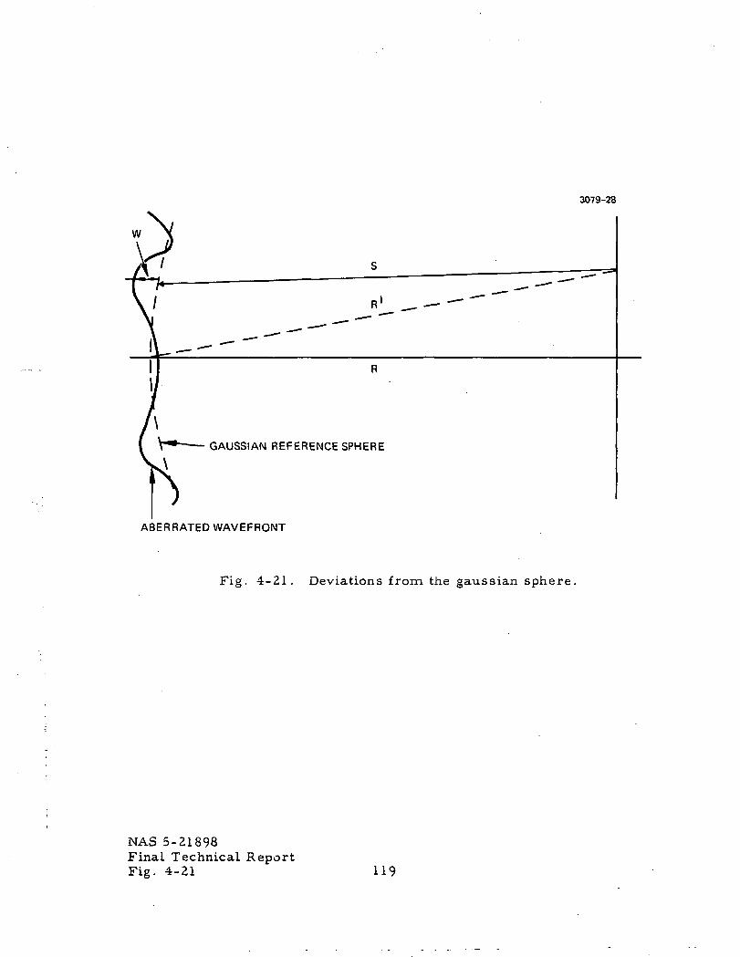
3079-28
W
GAUSSIAN REFERENCE SPHERE
ABERRATED WAVEFRONT
Fig. 4-21. Deviations from the gaussian sphere.
NAS 5-21898Final Technical ReportFig. 4-21 119
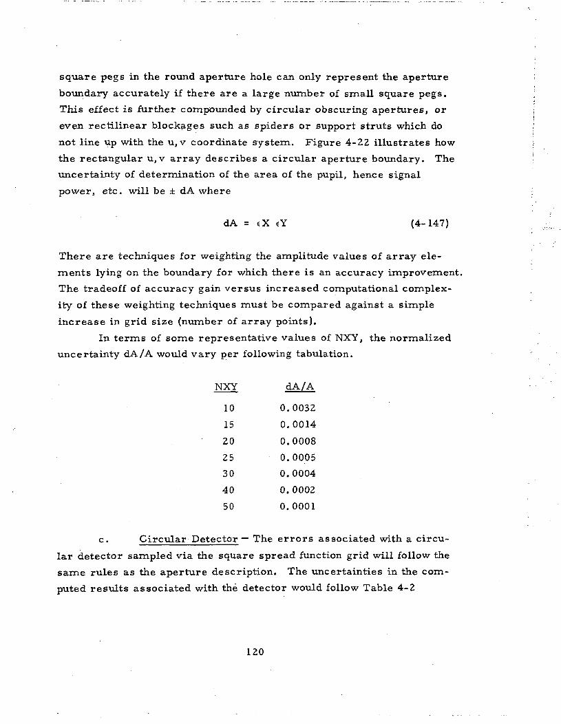
square pegs in the round aperture hole can only represent the aperture
boundary accurately if there are a large number of small square pegs.
This effect is further compounded by circular obscuring apertures, or
even rectilinear blockages such as spiders or support struts which do
not line up with the u, v coordinate system. Figure 4-22 illustrates how
the rectangular u, v array describes a circular aperture boundary. Theuncertainty of determination of the area of the pupil, hence signal
power, etc. will be ± dA where
dA = «X cY (4-147)
There are techniques for weighting the amplitude values of array ele-
ments lying on the boundary for which there is an accuracy improvement.
The tradeoff of accuracy gain versus increased computational complex-
ity of these weighting techniques must be compared against a simple
increase in grid size (number of array points).
In terms of some representative values of NXY, the normalized
uncertainty dA/A would vary per following tabulation.
NXY dA/A
10
15
20
25
30
40
50
0.0032
0.0014
0.0008
0.0005
0.0004
0.0002
0.0001
c. Circular Detector ~ The errors associated with a circu-
lar detector sampled via the square spread function grid will follow the
same rules as the aperture description. The uncertainties in the com-
puted results associated with the detector would follow Table 4-2
120
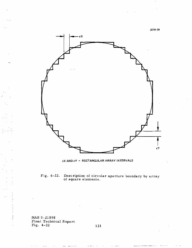
3079-29
eX
eX AND eY = RECTANGULAR ARRAY INTERVALS
Fig. 4-22. Description of circular aperture boundary by arrayof square elements.
NAS 5-21898Final Technical ReportFig. 4-22 121
with NXY replaced by IDIM. IDIM is the array size for the
detector.
TTYTTV/T Circular Detector DiameterIDIM = - 2 DELFS -
IDIM = IDETEC (2, J)
= 10 (Default)
d. Aliasing — The computed Fraunhofer diffraction function
is based on a discrete complex amplitude array (pupil function). This
discreteness results in a series of replicated, overlapping far-field
patterns as illustrated in Fig. 4-23 which constitute an infinite periodic
function. The spacing between these replicated patterns is directly
proportional to the array size or number of points across the pupil.
These patterns overlap so that each computed ASF or PSF value repre-
sents the superposition of all the replicated spread functions at a given.
point in the image plane. Thus, a point midway between two replica-
ted spread function peaks will have a value twice that of either spread
function plus a contribution from all the other surrounding spread
functions. The larger the number of sample points across the beam,
the greater the separation between these replicated spread functions,
hence, the lower the errors in the spread function due to aliasing or
overlapping.
Aliasing errors increase with aberration since the effect of
aberrations is to increase the spread function values away from the
center while reducing the central spread function values.
e. Effect of Defocusing on Aliasing — As indicated in
Fig. 4-23, the distance between peaks of the replicated overlapping
spread functions is Axrep and
Axrep = Z\ NXY f#
122

3079-30
\
X>^N/ Uw
• &X rep-
\
\
\
Fig. 4-23. Replicated (aliased) spread functions due to discrete sampl-ing of pupil.
NAS 5-21898Final Technical ReportFig. 4-23 123
where
X = spectral wavelength
NXY 5 number of grid points over entrance pupil semidiameter
f# = relative aperture
Aberrations and/or defocusing which cause geometrical spread
approaching Axrep will destroy the accuracy of these computations.
A defocusing AF resulting in a geometrical spread of Axrep would be
AF = 2 f# Axrep
= 4X NXY (f#)2
which is obviously excessive as would be a defocusing of half or one-
fourth that amount. It can be said, therefore, that to minimize aliasing
error due to defocusing
AF« X NXY(f#)2
and preferably
AF — 0.
f. LACOMA Test Case — Numerical Results — A test case
was devised to check accuracy. It consists of diffraction limited
received signal and L. O. optics. The relative aperture of the received
signal optics is 10, and for the L,. O. is 100. The matrix of optical
path differences indicates zero (10 ) over the pupil. The (complex
amplitude) pupil function indicates a uniform 100%. A peak value of
1. 0013013 rather than 1. 0 indicates a slight demagnification of the
exit pupil as used for the analysis. The ASF for the received signal is
real with a peak value of 73. 74928 compared to a predicted value of
74.0147
124
A = entrance pupil area
P = total input power
F = focal length
representing an error of 0.3%. Signal power is computed to be
65.6453 which compares with a predicted diffraction limited value of
65.82 for an error of 0. 3%. Both these errors are to be expected from
the value of IDIM = 10 and the predicted uncertainty of 0.0032 for
NXY = 10 per Table 4-2.
The local oscillator results were examined in terms of the peak
ASF value a . The computed value is 0. 8018 while the predicted value
is a =0. 8352. The 4% error here is due to the gaussian pupil function
changing rapidly at the edge of the aperture where the aperture sampling2
errors are thereby enhanced. The further the 1/e point is from the
aperture edge or truncation point (in either direction) the lower this
error will be.
Review of numerical results for the various sample cases indi-
cates that the above accuracy values represent a realistic range to be
encountered in the analysis of typical systems.
125

APPENDIX A
••• TRANSMITTER T?ST CASE •••IINP3 £ T A O ( i ) *?., .5, KID * ],., HID -a., a., XLINVIII =o.,:.NAu(l) -i..,j., IFLGK1) = w,u,RHOSI1I =j.,.Jl,0., D.,.J1,;.,TS(l) *G., ItQ.,U.,J.,1kJ.,u.,XMUS<1) = 0*1.,
MFRS = 10, OELFS = .LI,NXT = 25,JEMO
127 Preceding page blank i
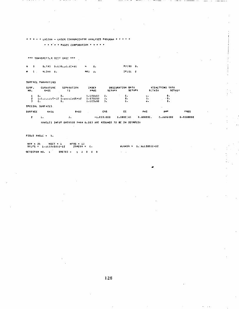
LACOMA - LASER CanMUNICATOR ANALYSIS PROGRAM
...'.. P4GOS CORPORATION .....
••» TRANSMITTER TEJT CASE •••
N 3 8:.TAO 5.UO..ji;,JE»l)0 H 0.
H C . XLINV 0. MA; 0. IFLG1 0
SURFACE PARAMETERS
SURF. CURVATURE SEPARATION INDEX OBSCURATION D A T A VIGNETTING O A T ANO. RHOS T5 XMUS 9 E T A P X BETAPT B £ T A S X BETAS?
I E . 0 .
3 C. 0.
SPECIAL SURFACES
SURFACE RHD1
2 L.
i . t o o u O J a.. • i tip + i ? i r i ft ii n i iJ b U U t + b c I c L J U U u J J •
1 . C C O I O O 3 .
RH02 CRS
} . - l . C C O J O O O
C.C.C.
CC
D . C O O C 1 C C
b •
C.
PHI
0 . O O O O O C .
0.• 0.0.
AHP
c. j o o o g o o
FREQ
0 . 0 0 0 0 0 0 0
(ANGLES INFUT GREATER THA.V 6.283 ARE ASSUHEO TO BE IN DEGREES!
FIELD ANGLc. = 9.
NX» = Z<, NDET = 1 NFRS = 13DELFS = l .u lOOUOi)LE-C2 ZOUEGA s C. VLAHOA - 1.:611385ut-Q2
DETECTOR NO. 1 IOETEC = 1 0 0 0 0
128
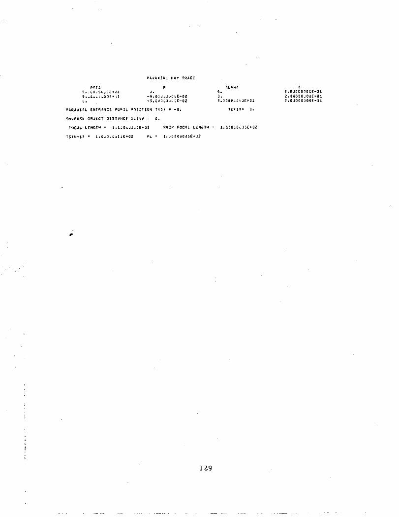
PiSAXIAL mi TRACE
PETA R ALPHA A5.. CO.CLjilE»Jt J. 1. 3.CJ00030CE-J15. .lull uO JE»-Jl -5.0 JJ^J JCOE-OZ 0. 2. 00000 J OUE-O I
E»01 3.0 J000300E-Q1
PAI?«XIAL ENTRANCE PUPIL POSITION T ( O I = -0. TE«IT=
INVERSE OBJECT DISTANCE XL INV = 0.
FOCAL LTNGTH t 1. L J Oi, J Ju uE» J2 BACK FOCAL LENGTH = I. DOG 1 Oil )CE
TS(N-l) = 1 . Cu J jl, jC j£»0i FL = 1. j C i O O u O J O E » J2
129
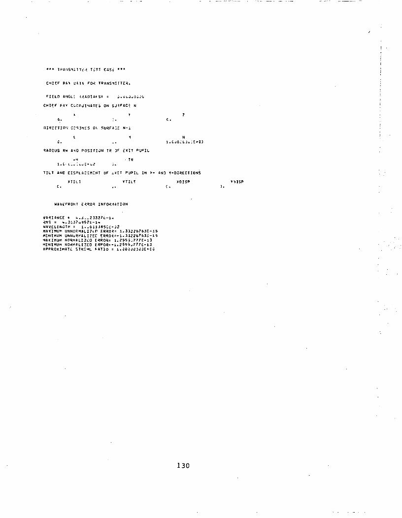
••» TPSMSIiTTc^ T£?T CAS£ •••
CHIFF pt\ U C T A FO< TRANSII fTEK.
FIELCI AN&L: (J.ioisfsi = i .o iOoCiJi ;
CHIEF F.1Y COCFJIN4TE5 ON SJ*Fac; N
> r 7o . : . c .
DIRECTION c:<5jN-s 01. SUSFA;; N-I
L 1 No. .. I.CJO;I.JU:E»O]
9»oius RH «MO POSITION TR IF inn PU^IL
iH • T*i.t. L.. :^.u •l,^ ;.
TILT AND CISBLaCEMTNT OF iKIT P'JPIL IN X- AN3 Y-OIRECT IONS
XTUT TTILT XOISP »TISPC. ,. C. 1.
KAVtFRONT t^ROR INFOK1ATION
VARIANCE =RMS = <..3C3HAVtLENuTH = l.a61J385S£- J2MAXIMUM UHNDRMALIZtn ER«0*= 1 . 33226763E-1 5MINIMUM UNNO^rALIZEC ERRO<=- 1 . 3 J2Z6763E- 1 5MAXIMUM NORMALIZtD E«ROR= 1 . Z55 5 J 7 77 E- 1 3MINIMUM NORMALIZED ERPOR=-1. 3555a777£- 13APPROXIMATc. STREHL fATIO = 1 . 30 j Ji)3 J3£»C3
130

••• TRANSMITT£S TiSI CAS; •••
TR&NSHITUR RAT&,
PEAK INTENSITr = t.U1223l9£»wlOPTICAL TRftNSMSSION = 9. J-tS68a6£-01 ( -.COZ 09 1MtXIHUH UNTiNNA GAII = 8.73ll9b9E» J6 ( 69.mi OR )OVERALL TRSNSHTTEP. £FFICI£NCY = 9.32df 7 33E-t t ( -.31-9 OB )
131

APPENDIX B
TRANSMITTER TEST CASE •!I1NP BETAim = 2.25, Hdl = J., IFLG1C1) = 0, N(l) = -7,RAOSUITS ill 3
ZOMEGA =XftUS (1)S K A P A ( S )C«S(6) =
- i .
0.9s 1 .
-1.
VJ.ftSSZ, t>/ r.b55^'., 0.,-l^Za.,8.
5,
t
MfRS = 51, !5ELFS = 50,t£NO
133 Preceding page blank
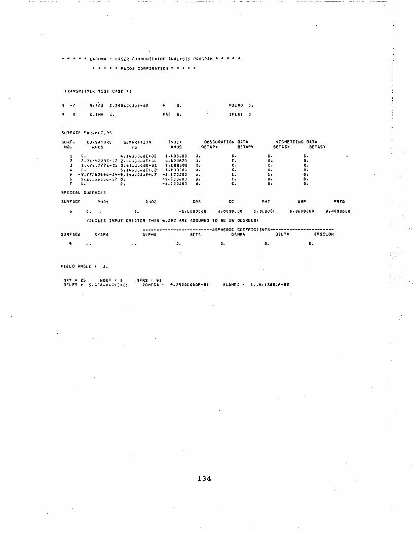
LCCOMA - LASER CJrlMUKlCarOR ANALYSIS PROGRAM
• • • • • PAi05 CORPORATION • • • • •
T Z A N S M I T T E * TIS1 CASE »1
N -7 Ri lA jJ 2 . ? 5 0 0 J Q J J £ » J O
" 0 XLINV u.
M 0.
MAG 0.
PZCRO 0.
IFLG1 0
SURF. C U R V A T U R E S E P A ^ A T I O * INDEX OBSCINO. «HCS ri XMUS R E T A P
1 G » 4 * . l > * j j 3 ; *3E t02 l . C O O w O O J.
3 l«;,/6,j77^£-Ci S.bllJi jbJE^Ol l . C Q O b O O 3*<« C» S . l ^ * j J jo3E + o2 l i C O O C O M U.
7 (,, 0. -1 .100JOO 0.
JRATION DATA VIGNETTING 0X 6ETAPV B E T A S X
C. C. 0.C . 0 . 0 .C. C. 0.E. C. 0.E. C. 0.C. 0. 0.C. 0. 0.
SPECIAL SURFACES
BETAS*
SURFACE
6
SURFACE
5
PM01 RH03 CRS
- l . t O O J O u O
cc
u.0000:011
PHI
o.o iooo; .
(ANGLES INPUT GREATER THAN 6.263 ARE ASSUMED TO BE IN OEGREESI
SKAPA ALPHA BETA
I. ;. 3.
AMP
C.3COOOOO
ASPHERIC COEFFICIENTSGAMMA OELTA
FREQ
0.0000000
EPSILON
FIELD ANGLE =
NXY = 25 NDET t 1OELFS = 5. O t O y U i i u ( E » 0 1
NFRS = 5120MEGA = 9.2500tO( iOE-01 V L A M O A 1. j61138SiJE-02
134
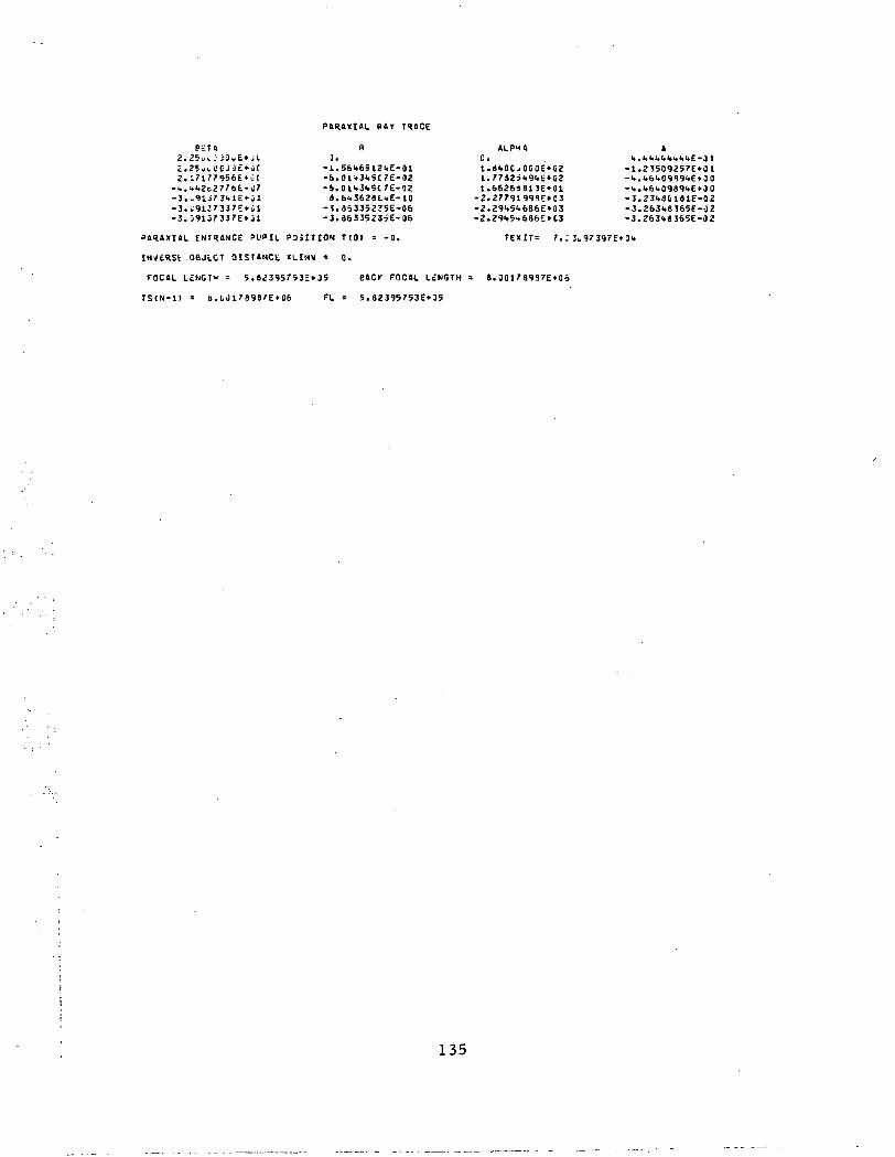
PARAKIAL PAY TUSCE
P=TA B ALPHA A2£ui ; : jOo£»Jl J. C. "t.<."»<.<.lt<«<«<»£-;]l
l t . i < t ( JO jOOOE»03 -1.23509257E»01Z 1.77i2i".9<ii; »OZ -i.<>6l.09<i9<.E»0 0Z 1.6626481 J£»01 -t>.i>6<»09a9i>E»l 0
-3..91J73'.lE»jl 8.6".3628L*E-tO -2. 27791 99NE»C3 -3.231.86 181f -0 2-3.i.9137337E»ul -1.8S3352JSE-06 -2.29".5'»686E»(13 -3.263".8365f-0 2-3.09157337E»J1 -3.8633S237E-06 -2.29".5-,i>86£»CJ -3.253".8365E-0 2
P4HAXIAL ENTRANCE Pt'PIL POSITION T ( 0 > = -0. TEXIT= 7.; Ji. 97397E* 3<>
IMVtRSt OBJLCT QISTAMCt X1.IMV - 0.
FOCAL L£MGTH = 5 .8239S753£»JS BACK FOCAL L£MGTH - 8.a01789S7£»06
TS(N-l ) = B.LJ178987£»06 FL = 5.82395753E*:S
135
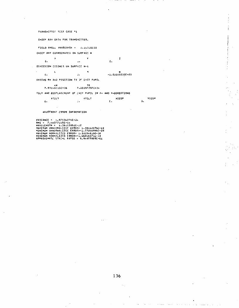
TRANSMITTED TEST CtSE •!
CHIEF RAY D6T6 FOR TRANSMITTER.
FIELD ANDLL (RAOIAKSI = u. jijjj0.no
CHIEF RAY COORDINATES ON SJRFAC; N
X Y Z
0. -. C.
DIRECTION COSINES ON SURFA:E N- 1
L I NG. J. - l .C ' JC00030E»CO
RADIUS RW ASO POSITION T^ 3F EXIT PJPIL
^H TR7.93li.6C13£»36 7 . 0
TILT «NO OISDLAC£M£NT OF £<IT P'JPIL IN X- AND Y-OIRECTIONS
>TILT YTILT XOISP
HAVEFRONT £<?"?OR INFORMATION
VARIANCE =RMS = 7.fcS377uii5E-lii.WAVELENGTH = I.]bll385i)£-j2MAXIMUM UNND^MALIZET ER»0^= 1.3811Za?6£-10HININUM UNNORMALIZ£C ERRO*"1 . 77fl<.6895£-05MAXIMUM NORMALIZED E*ROR= 1. 3J151.8 J»E-36MINIMUM NORMALIZED f *ROR = -1. 668i.6171t- 33APPROXIMATE STKEHL SATIO = 9.9^?77899E-C1
136

TRANSMITTER TEST CASE »1
TRANSMITTER OATA.
PEAK INTENSITY = 1. 1.16?JJUE-07OPTICAL TRANSMISSION * 9.999998'.E-a 1 ( -.COO 09 )MAXIMUM ANTENNA GAIK = 3.3319166E»08 ( 95.337 OS IOVERALL TRANSMITTER cFFICIiNCY > 3. 366C7 71.E-01 ( -1..739 09 )
137
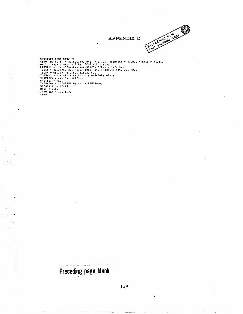
APPENDIX C
RECEIVER TEST 3ASE 'It INP B c T A i d l = 82 .5t l .34 , H ( l > = U . . C . , X L I N V ( t ) * l i . t O . , « A G ( l )N i l ) - -9, -7, M ( l ) = 5,6, I F L & K U : 1,0.R A O S ( l ) = ... -320. ,0., 1.1.80175, 6*0., 111.2, 0.,TSUI e 3bb .72S, 0., -5;a.9J985, 1*6.11.387,96.1.25, 2., -2.,T S I S ) = 5b.775, 0.. 0., 111.2. C.,X M U S I 1 I * 1.. -1..-1., 1., I.. u . J O O b Z i 6*1..S K A P 4 I 2 ) * u., 1,, .71736,CRS<11) = -1.,T H T A » ( 6 ) = -.78539616, <. . , -.78539816,B E T A P X ( l ) = 12.1.5,
I P R O G ( l ) = 1,1, 1,J,SEND
Preceding page blank
139
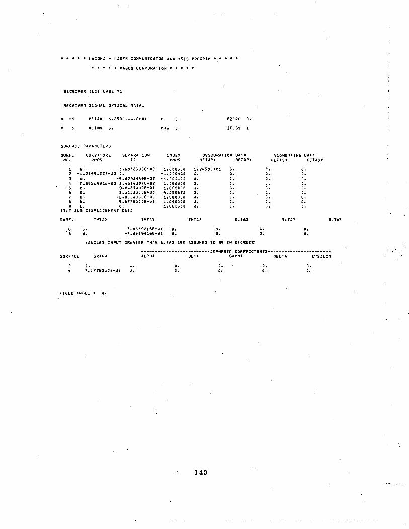
ISCOMA . LASER COMMUNICATOR ANALYSIS PROGRAM
..... pfljos CORPORATION .....
RECEIVER TEST CASE •!
RECEIVED SIGNAL OPTICAL TATA.
N -9 BETAO 8.250CU.«uE»01
M 5 XLINV C.
P2ERO 3.
IFLG1 1
SURFACE PARAMETERS
SURF.NO.
12 -3
56789
C.1.0.7.C.0.0.0.C.
TILT AND
SURF.
6' 8
SURFACE
24
Iu
CUkVATURE SEPARATIONRHOS T;
3.b8725J6E»022195122E-J3 0.
11
-5.029J4B5E*32 -105Z..991E-03 l.»&l»J87E»G2
9. 8*25 JOOE*0 12. jtjJJw JE*CO
-2.0C3uOOOE*0-G5.6775000E*ul0.
DISPLACEMENT DATA
THTAX THTAY
7.6S39816E-J1-7.d539816E-01
(ANGLES INPUT GREATER THAN fe
SKAPA ALPHA
C. u.7.l7363udc-Jl J.
11k111
•
INDEXXMUS
.COOjOO
.030JOO
.(.00.33
.COOOOO
.COOOOO
.C30&23• t 0 OJbil.COOOOO.(.03-jOO
0.0.
263 ARE
0.0.
OBSCURATION DATA VIGNETTING DATARETAOX
1.2«.50E»C1U •
3.3.J.3.3.J.3.
THTAZ
C.0.
BETAPY BETASX BETASY
0. C. 0.0. C. 0.C. C. 0.C. G. 0.C. 0. 0.C. C. 0.C. 0. 0.C. C. 0.C. i.. 0.
OLTAX 9LTAV 0!
C. 0.3. 3.
ASSUMED TO BE IN DEGREES)
BETA GAMMA DELTA E"SILON
0. .0. 0.0. 0. 0.
OLTA?
FIELD ANGLi = J.
140
LOCAL OSCILLATOR CPTICAc 1ATA.
N -3 9tTA^ 1.39000;jJ£»3C
M 10 XLIHV o.
H 0.
MAG 0.
P7zRO 0.
IFLGl 0
SURFACE °6«tMETESS
CUKI/ATtmSURFNO. T3
INDEXXHUS
l . C O O O O - Jl . C O O O O OL.lQOOilO
03SCU9A!S E T A P X
].J.}.
riOM D A T A9ETAPY
C.C.a.
VIGNETTING 0B E T A S *
^. 0.c. a.0. 0.
BeTASr
10 C. 0.11 6.S9i:3-j5d£-J3 l.llZJuJiiE*.i.2 C. C.
SPECIAL SURFACES
SURFACE RH01 11H02 CHS CC PHI
11 i. j. -i.coojoao j.ooocaoo o.joouo^.
(ANGLES IMFUT GR£AT£R THAN 6.283 ARE ASSUMED TO BE IN DEGREES)
AHf» FREQ
0.0)00000
FIELD ANGLE = (,.
NXY = 25 N3ETOcLFS = •:.
NFRS = 26ZOMEG9 : C. VLAMOA = l.;611385iE-02
DETECTOR OtTA.
DETECTOR NO. 1 IDETEC 1 J 0 0 0
141
P1RAXIAL PAY TRACE - RECEIVED SIGNAL OPTICS.
B E t a
B . Z S C - u l . J £ * t l
-3.<.1892e53E»Cl- 3 . 3 e 7 7 - . 2 2 j E » O t-3 .b l2b? f9 . i t»U
B
-2. J1219512E-01-Z.J1219512E-01
6.Z-.6231.92E-026.2»6Z3i»92£-02
&.2-.6231.92E-02o.2<->23i.92E-02
A L P H A0.
».1>693939<>E»CO5 . 0 8 3 0 7 0 J 5 £ * C O
-5.Z16C?6iOE»Ki-l .Z15228C2E»01- i . z t a r s t c^Eto i-l.63t763S5£*01
A1.2121Z121E-321.Z2025129E-031.22025129E-33
-7.0»723806E-i)Z-7 .0 I . 7Z3RO&E-OZ-7.0".7Z3?06E-a2-7.0".7Z3506E-J2-7.0-.723806E-02-7 .0*7Z3aOE>E-3Z
P A ^ A X I A L ENTRANCE PUPIL P03ITIOS T ( 0 > = -3. 7lt 927h2E»S3 TEXIT= -9.S 92<t9ZZ6E»0 1
INVERSE OPJE.CT 3ISTONCE X.INV = ii.
FOCAL LEMG1M = -1.12P795b:i£*03 BACK FOCAL Lttl&TH = 5.62359C'6E*01
TSCN-l l - s . f c T ^ S O ^ L j £ » e i FL = -1.3Z079SbtE*)3
142
P A R A X I A L PAT TRACE - LOCAL OSCILLATOR OPTICS.
E t T A 9 ALPHAl."90,.C UJ£»ul ). 3.t.39b<.,KuUE»u t - 1 . 2 5 J C ' l a C O E - O Z J. 7.11UZ1.U60E-01I.»il..85it7£-lfc - l . Z5JDa jCOE-02 9.0000 i 0. 0£»01 7 .19fcZ»<.60E-i) 1
P A R A X I A L £HTf<ANC£ PUPIL POilflON T ( 0 ) = -0. TE»IT= 0.
INVERSE oejerT DISTANCE XLINV = o.
FOCAL LcNOT" = 1. 1121.„»« i£» J3 BACK FOCAL LENGTH = 1. 11ZOG. KE^O!
TS(N-l) = 1.1120CH^E*32 FL = 1. llZOOOOt EKiZ
143
RECEIVER TtST CASE •!
CHIEF RAY DATA FOR REC£IV£3 SIGNAL.
FIELD ANGL£ (RADIANS) = g . 000-0.1 JO
CHIEF RAY CDOROINATFS ON SJRFACZ N
» 1 70. 1.16u2539iE*00 C.
DIRECTION COSINES ON SURFAI£ N-l
L M N0. -7.1i,»i.Z73oE-li< l.OOCOOOOCE'OO
RADIUS RM AND POSITION TR DF EXIT PUPIL
RH TRi.536999i3E»02 -'*. 692«. 9225£»B1
TILT AND DISPLACEMENT OF KIT PUPIL IN X- AND Y-OIRECTIONS
XTILT TTILT XOISP YO ISP0. -7.1.51.27ISE-1'. C.
UAVEFRONT ERROR INFOR1ATION
VARIANCE = 3.B«398(l<9E-J2RMS = 7.*7fc68726E-t2WAVELENGTH = l.u611365JE-jaMAXIMUM UNNDPMALIZEO ERROR= 0.MINIMUM UNNORHALI7EP ERROR=-1.6*265"»96E-03MAX.IMUM NORMALIZED ERROR= J.MINIMUh NORMALIZbD ERROR=-1. 5".8Jl. OilE-01APPROXIMATE STR-HL PATIO s 7.S5191571E-C1
144
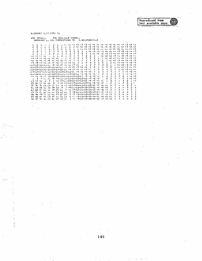
Reproduced frombest available copy.
T L T T cas;
( P E 4 L ) ,ICC,
SIGMA:..3 TO 1. 3C " E»'j3
I2S21
-11-
13
37
75
93
i i2 i-j j2 i'1 1
I t i - l J --". -5
3 ?13 112". z:3t 3-1.9 U662 5.17". 7.a"» 7992 a'
C.
<
010
bi7 c
i
33i.
12-3- j
5U
* •*12
l2T
321
-13--10--5
18
17
!5
1
13c
1 12 HJ 33 i
-11233
•)
1--13-13-11
12-13-1«-1<*- •J - i l - i i -m
1 JId25
(. ,,
*• *
9 J10 7£.1 112' 15
1
-5-1
?1d
1 2 2 3 3 3
-U -9 -6 -<• -2 C
-13-12-1J -t -6 -3-1I.-13-12-10 -7 -5
i ^ m i zlj l* :, :' °-l.-13-l'5-15-U-ll-7-12-l^-l5-li.-12-5-11-1-.-1S-15-13--3 -9-15-15-15-1".-
• » i<i if,
1
2.!5
-t
-2
!
-s-9i :•11
**"*
i23
J21
-5-6-7-7
"*
•J
1
2
?221
-2-3-1
G1
33332
10
- j-1
1
'
"*
j
33
I
21
» T
J
333
i
-3
012333
uU
U
U
U
_
• I*
-1
1122333t*i*c*L
-5 -5
-2 -U-2 -J-1 -2
C -11 - .2 t2 02 13 13 13 21 2
145
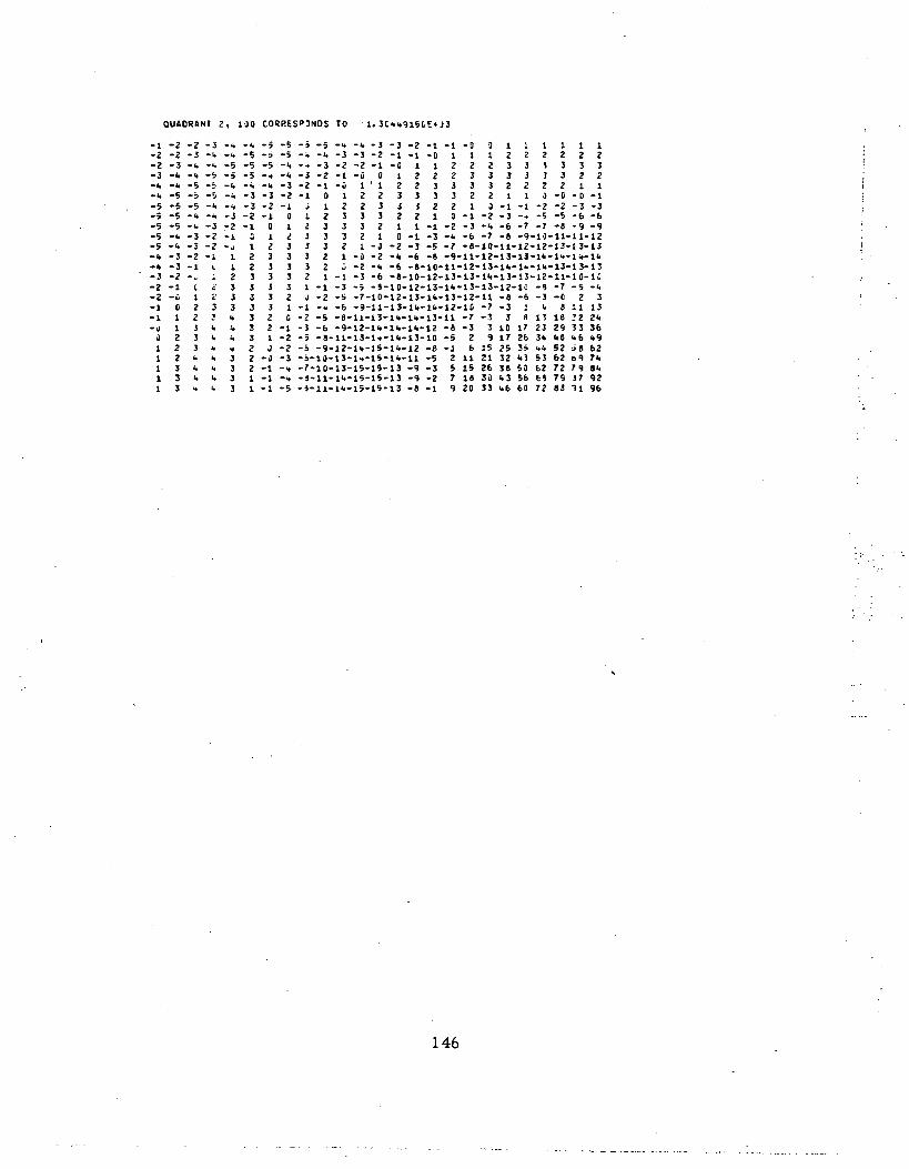
QUADRANT 2, 1JO CORRESP3NOS TO 1. 3C<.<.9151 Et J3
-1
-*»•*»
'
-5-"»-it-3-2-2-1-1
0111
1
-2
-i.-5
-"•-3-3-2-1-0
01
2223
3
-2
**
-3-2-1
C12Z
33ui.
t*
-3^
-t.
-2
L
t
3T
t.
w
-J*
-*»
112333**
t**»33
3
-*»
-3
12233333
3222
1
-5 -5 -
-i. -3 --3 -2 -
3 33 33 31 33 23 1 -2 C -
1 -2 -
-J -3 --1 -» -)
-1 -5 -:
> -5 -» -«. -3 -3 -2 -1 -1 -5 0 1 1 1 1 1 1
! - l - u l ' 1 2 2 3 3 3 3 2 2 2 2 1 1L 0 1 2 2 3 3 3 3 2 2 1 1 J - 0 - 0 - 1
J 3 2 1 -J -2 -3 -5 -7 -8-10-11-12-12-13-13-13! 2 1 -0 -2 -«. -6 -8 -9-ll-12-13-U-li.-lt-li.-li.! 2 0 -2 -i. -6 -8-10-11-12-13-1I.-1I.-1I.-13-13-13! 1 - 1 - 3 -6 -8-10-12-13-13-11.-13-13-12-11-10-1C
-1 -3 -5 -9-10-12-13-11.-13-13-12-10 -» -7 -5 -«.-2 -S -7-10-12-13-1I.-13-12-11 -8 -6 -3 -C 2 3-H -6 -9-11-13-H.-11.-12-1C -7-3 1 k 811 13-5 -8-11-13-1I.-11.-13-11 - 7 - 3 3 a H 16 22 2".
-8-ll-13-l»-lii-13-10 -5 2 9 17 26 3fc i»0 ".6 49-9-12-li.-l5-li.-12 -8 -1 6 IS 25 3i fcV 52 i8 62
-ll)-13-lH-15-ll.-ll -5 2 11 21 32 1.3 53 62 o9 71.-10-13-15-15-13 -9 -3 5 15 26 38 50 62 72 79 »t.
-11-1I.-15-15-13 -8 -1 9 20 33 U6 60 72 83 11 96
146
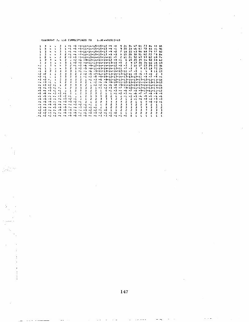
QUADRANT j, 1JO CORRESPONDS TO t.JCHU915CE»D3
11
111]
-J-1-1-2-2-3-4-*•-5
-<*
'
-1
33
3222110
-c-1-2-3-3-<.
-5
**
-2
i*
^H
3}Ji;
21•„
-1
-^-3
_
-5
**
*
*.*i*•*t.j3•e.1i
-1- £.
14
'
T
3 13 1
3 Z3 3<• 3<* 3*» 3* 33 33 33 32 31 ZI 3
1
-» -3
-** -u
-I-1
-1-J
J
122333s132
-3
"*
-5-5
-J-11-1<.-15-15-12 -8 -0 9 21 3U H7 61 73 8". ?3 99-S-11-1W-15-1S-13 -» -1 9 20 33 >»6 6! 72 83 U 96
-i, -/-1J-13-15-15-13 -9 -3 S 15 26 38 5i 62 72 '9 8U-3-2-2-1
01233333
*
-Z
-5
-b-U- 13-1<«-1S-1<»-11 -5 2 11 21 52 <>3 53 62 o9 7U-o -9-l2-tl»-lJ-l'.-12 -8 -I 6 15 25 35 ".". 52 58 62-i -d-ll-l3-li.-l<.-13-10 -5 2 9 17 26 3". i>0 ->& ".9-3 -6-Z -5-I -i.
J -2I -12 13 23 23 3
-1 J
-5 -5
-9-l2-l»-l»-li.-12 -8 -3 3 10 17 23 29 33 36-a-ll-13-l".-l<»-l3-ll - 7 - 3 3 S 13 18 ?2 2".-6 -9-lt-13-l<.-ll.-12-10 - 7 - 3 1 "t 8 11 13-5 -7-1U-12-13-1U-13-12-11 -8 -6 - 3 - 0 2 3-3 -5 -S-10-12-13-11.-13-13-12-1Q -8 -7 -5 -".-1 -3 -6 -8-10-l2-13-13-li.-13-13-l2-ll-ia-10
L -2 -"• -6 -9-lO-ll-12-13-ll.-l".-l*-13-l3-131 -0 -2 -". -6 -8 -9-ll-12-13-13-l<.-H,-li.-ll,2 1 - 1 - 2 -3 -5 -7 -5-10-11-12-12-13-13-13
1 2 2 3 3 3 3 2 2 1 1 3 - 0 - 0 - 1
147
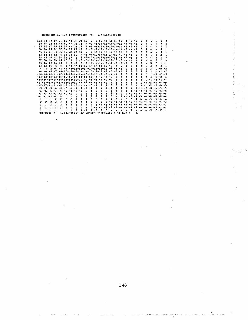
QUADRANT >,, 130 CORRESPONDS TO 1. 31 fcl.91SOE«03
100 98 9? 8i> 7o98 97 92 83 73
86 8". 79 72 £275 71. 7C 63 i*63 62 58 Si ".".S3 1.9 <i6 1.1 31.37 36 3<> 29 2325 2<t 22 Ib 1313 13 11 8 5l. 3 Z - i - 3
-» -l. -5 -7 -8-io-ii>-ii;-ij-i2-13-13-13-13-11.-lit-lit-llt-lt-Jit-H-13-13-13-13-12-13-11-11-13
1 1 1 2 2
I N T E R V A L = 1
62 ".8 3". 21 10 -„ -7-12-15-16-1I.-126C <•/ 33 21 9 -u -6-13-15-16-111-12
51 39 27 15 5 -3 -9-1 J-lS-15-lfc-ll<tit 33 22 11 2 -&-11-1H-15-15-13-1335 25 16 ' -1 -7-i2-l»-15-l*-1226 18 9 2 -5-10-13-15-15-13-1117 U 3 -I -8-12-l»-l5-l<.-12-108 3 - 2 -7-ll-13-i»-l<-13-ll - 81 -3 -7-13-l2-l«i-li.-13-12 -9 -7
-5 -S-ll-12-l»-l«.-13-12-10 -7 -5-1C-12-13-1<-H.-13-12-13 -8 -6 -3-J3-13-IV-1V-13-12-13 -» -6 -* -1-1I.-14-13-13-11-10 -8 -6 -<i -2 0-13-13-12-11 -9 -8 -D -fc -2 -0 1-12-11-10 -8 -7 -5 -3 - 2 - 0 1 2-9 -8 -7 -b -". -3 -1 0 1 2 3
. 03o295l,5t-32 NU19ER I N T E R V A L S *
-9-8-7-5-*-2-1
02233
51
-8-8
-7-7-6-5-t.-2-1
0123333
**
SUM
l l
n ui
vn
-i.-3-3-2-1
012233332
-2-2
-1-0
011233333321
0.
11
22233333333210
31
333i«ItItU33221
-0-1
'
i,it
ititit(,fc333210
-1-1-2
itit
iti*3332211
-8-1-2-3-3
33
3322210
-0-1-2-2-3-it-i.
22
111I'0. ;-1-2-2-3-ii-u-5-5
148
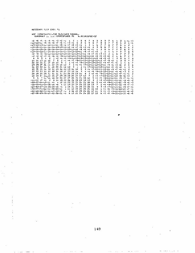
RECEIVER HST CAS; *i
f t S F t l M l f l N S P Y ) ,FOF R c C d l i f E D SIGNHL.OU40P4M 1, In) CORRESPONDS TO b. 0 1083078E»OZ
-lli-10-lu -9-11-13-13-U--15-15-1S.-1".-
-912m
-8 -7 -6-11-11 -9- 1"»-
- l".-l<t -15- 15-15 -1S--12-12-12-1;-
-2 -2 -2 -36 e e ,O p <•
1» 1". 13 1222 22 21 2t29 29 2S 2t3» 33 33 3i35 35 35 3U33 33 33 3328 28 28 2918 18 2C 21N5 b 7 nx
-U-1C -7 -i-28-27-2".-!*-
1-6? S7 Jq-78-77-71-61--99-<J8-82-73-
n
-52
1017£1,
*£3333Tj
£3m
211
-1".-
-6
71522283132312613
8-i.
13- 12-
-l i <:-« -3 -1-1 -7 -511-10 -d
{j-3-7
1»-1'«-13-12-11-10!•.-!<.- 1«-1"»-13-
a2
-1-5-3
D ^ o a o o r b" . 5 6 7 8 8 7 71 3 " t b 7 7 8 7
- 3 - 0 2 3 5 6 7 7-6 -". -1 1 3 5 6 7-9 -7 -l» -2 v 2 l. =>
-i -9-11-12-13-13-13-12-11-1C -3 -5 -3 -0 2
5 212 919 1525 2129 2631 2931 3027 2922 25!"• 19
» 12_e. i.
» q _ . i n _ « c . _ i _
51hi
-97-95-89-79-67
— & W 4 W —
-38-23-11-",7--52-
32-1736-21
-I -"» -73 1 -2
12 7 3Id 13 923 19 1".i.1 23 192J 26 2329 28 2527 27 2623 2b 2613 23 25. ) | Q 5 TI . 1 7 C i
3 15 2 11 11 Id
-« d 16-5 6 15
-9--5-I
«10l<»1 9222"»252o' 7>(^
232221
11--8--"»
J59
l<t172J232<.2 q25
25252".
12-13-12-11-10 -7 -5 -210-12-12-12-11 -9 -7 -".-7-10-11-12-12-11 -9 -6-"• -7-10-11-12-11-10 -S
0 -". -7-13-11-12-11 -9u -j -5 -8-10-12-11-108 3 - 2 - 6 -9-11-12-11
12 7 2-3 -7-10-11-11
5 b7 57 67 77 76 7". 63 51 3
-1 1-3 -0-5 -2-7 -U-8 -6
-10 -7-10 -8
16 13 5 -D -5 -8-11-11-11 -918 13 8 2 -3 -7-10-U21 16 10 5 -1 -5 -9-11cc 19 13 7 1 ~*» — 8*10
2"t 21 16 10 ". -1 -6 -92"» 21 17 11 5 -1 -5 — )
-11-10-11-11-11-11
12i.5677765t.21
-1- 3- <*-6-7-8-9- 9
-11-11-10-11-11-1 0
2U 22 17 12 6 -0 -5 -9-11-11-10
-112t.5b777765320
-1-3-4-5-6™7
-7-8-8
-3-1
12t.5b787765.,j2y
-1-2-3- 3
-u-5-5
149
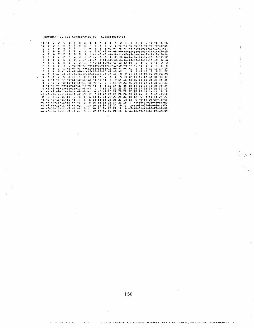
OUftDRANT i', 100 CORRESPONDS TO 6 . O C 0 8 3 0 7 6 £ » a 2
-3
2t.S6777765it
C
-3
-1
2
5677776532a
-2
-6
J 2
5 66 77 77 77 66 i5 3l. 22 -11 -2
-1 -»-3 -6
-5 -e-
i.
7776531
-1-3-5-7-8-
1J-
-9-11-11-
-i. -7-10-11--i. -7- IJ-ii-
1111
5
776t.2J
-2
7 6 6 8 8 7 6 5 It 2 1 -1 -2 -3 -i -5 -5 -6 -6
7 6 5 i. 2 -0 -2 -i. -6 -8-10-11-12-13-1. -li.-li.-l 5-156 5 3 1 - 1 - 3 - 6 -8-ia-ll-12-13-li.-l'.-15-lS-15-15-H.•» 3 j -2 -<• -7 -9-10-12-13-H.-K-H.-H.-1I.-13-13-12-122 C -2 -5 -7 -9-11-12-13-11.-11.-13-13-12-11-10 -9 -8 -81 -2 -5 -7 -9-11-12-13-13-13-12-11 -9 -8 -6 -5 -3 -2 -2
-2 -5 -7 -9-11-12-13-13-12-10-» -7 -9-11-12-12-12-11
-<. -7 -9-11-12-12-12-10-6-8
-8-10-12-12-11-10-10-11-12-11-10 -7
-8" "4
-9-11-12-11-10 -8 -* -i)10
11
10
-9-9
-11-11-13 -8 -5 -1
-11-lu - 7 - 3 1 7
-A -i. 1 6 12 15
-6 -1 5 11 16 21-5 -J i 11 17 22
12
1 A1 07 ilC U
22j ȣ i
2±*.
2<t
-8-5-0
l.9
17? fl£ U5 9£ £
25
?jj
252%
-9-5-1
t.9
lit« a1 021yi.£1Z ~72525| *
2222
-7-239
11.19
2526
2523
1 QI. 7
1716
-9-i.17
131823
2727
2319
86
-7 -l. -2 3 2 fc 5 6- 1 2 5 7 10 12 13 I f c
5 8 12 15 17 19 21 2211 15 19 22 2I> 26 28 2917 21 25 27 30 31 13 3323 26 29 31 33 3". 35 3526 29 31 32 33 33 33 33? A X fl T 1 Til Tfl ?Q PA * Ato -JU J 1 JU OU c? £3 CO
29 29 27 26 21. 21 JO 1827 25 22 1ft 1** 11 ft 623 19 H* 1 2 *3 ~7~10IB 12 5- *3 ™ 1 1* lfl~2 **• 2713 1. -5-15-25-3*--. 0-«.5
\ Tn-Jt '^T-siIfcjI / i Tfc-J>16-31-«.6-b 3-72-92-88-6-20-35-51-66-79-1)9-95
150
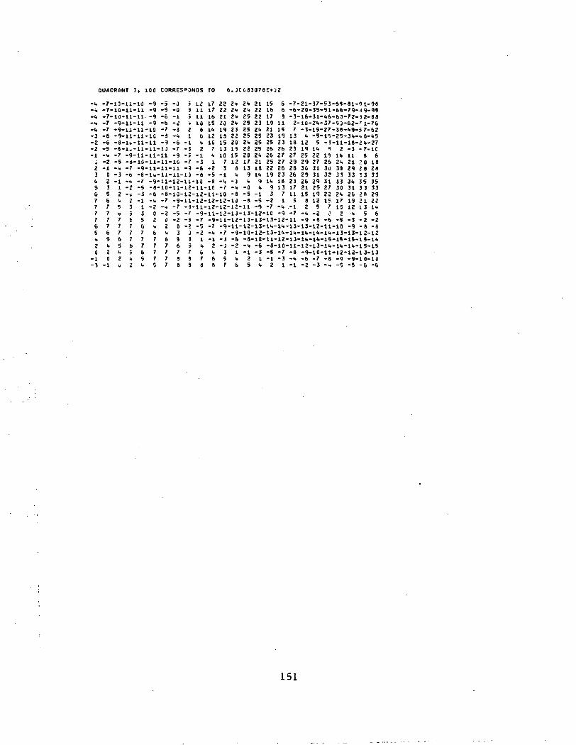
QUADRANT 3, 100 CORRESPONDS TO 6.JCuS3078E*J2
"*»
-It-3
-2-1
**3l.56777765<*20
-1
-7-10-11-10-7-10-11-11-7-10-11-11.
-7-6
-5-it
02356777765it20
-9-11-11--9-11-11-
-8--7
-112i.5b77765u2
11--9-11-
-i»-2•v
235677765
-5-3-1135677765
-9 -5 -0 i 12 17 22 2» 2* 21 15 6 -7-21-37-S3-5»-Sl-a 1-98-9 -5 -0 5 11 17 22 2* 2". 22 16 6 -6-20-35-51-65-79-;) 9-95-9 -6 -1 > 11 16 21 2i» 25 22 17 8 - 3-16-31-1.6-63-72- ) 2-88
10 - 7 - 3 2 8 11. 19 23 25 2* 21 15 7 -3-15-27-38-1.9-57-6210 -3-1. I 6 12 It 22 25 25 23 19 13 <. -S-1S-25-3".-'. 0-itS
11-1J - 7 - 3 2 7 13 19 22 25 26 26 23 19 1". 1 2 -3 -7-1C11-11 -9 -5 -1 i. 13 15 23 21. 26 27 27 25 22 1? 1* 11 86
-9-11-12-11-13 -8 -l. -3 it 9 1". 18 23 26 29 31 33 3d 35 35-8-10-11-12-11-10 -/ -i. -0 ". 9 13 17 21 25 27 30 31 33 33-6 -8-10-12-12-11-10 -8 -5-1 3 7 11 15 19 22 2". 26 £» 29-i. -7 -9-11-12-12-12-1J -8 -S -2 1 5 8 12 15 17 19 21 22-2 -"• -7 -9-11-12-12-12-11 -9 -7 -* .-1 2 5 7 1C 12 13 !<•
0 -2 -5 -r -9-11-12-13-13-12-10 -9 -7 -<» -20 2 •<. 5 62 0 - 2 - 5 -7 -9-11-12-13-13-13-12-11 -9 -8 -6 -5 -3 -2 -2<» 2 0 - 2 - 5 - 7 -9-ll-12-13-l'.-l'.-13-13-12-ll-10 -9 -8 -86 <• 3 i -2 -<• -7 -9-13-12-13-l"t-li.-li»-l<.-l<.-13-13-12-127 6 5 1 1 - 1 - 3 - 5 -8-10-11-12-13-11.-11.-15-15-15-IS-1'.7 7 6 5 ". 2 -d -2 -<• -6 -8-10-11-12-13-1".-!".-!'.-! 5-157 7 7 7 6 ". 3 1 - 1 - 3 - 5 - 7 - 8 -9-10-11-12-12-13-13
151
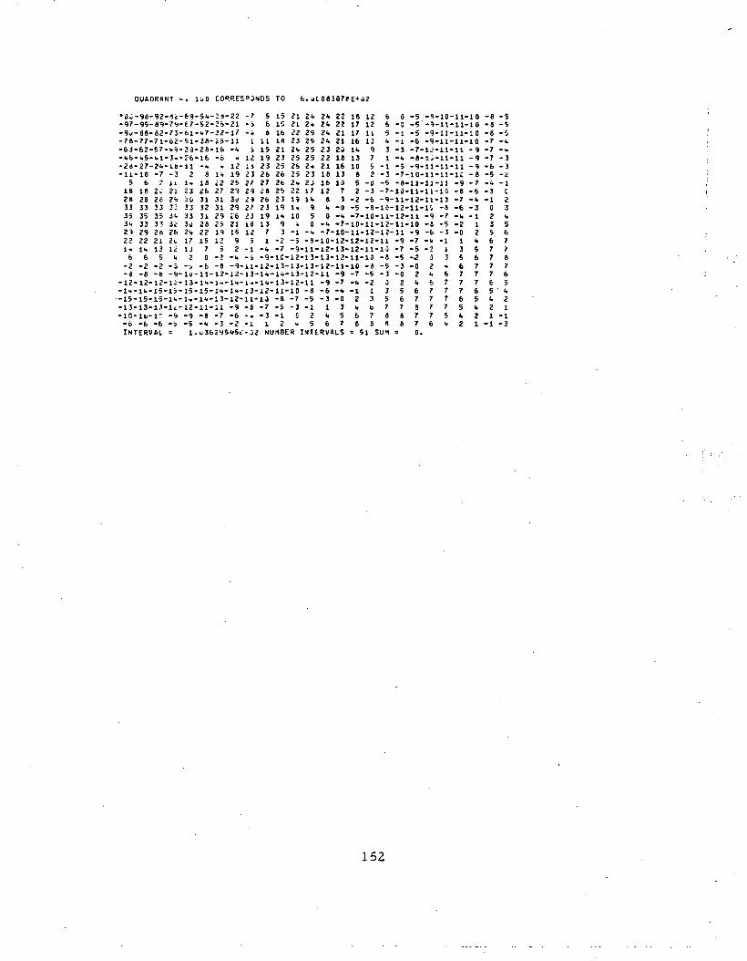
QUADRANT •., i^o CORRES°3NOS TO 6. Hi 08307S E*ii2
•i)l;-98-92-'i<!-fc9-5'.-3:>-22 -7 5 15 21 2<» 2<t 22 18 12 6 0 -5 -9-10-11-10 -8 -5-97-95-89-7'a-e7-52-3->-21 -b 6 10 21 24 2<» 22 17 12 6 -0 -5-9-11-11-10 -8 -S-9J-88-62-73-61-1.7-J2-17 -« 8 Ib 22 25 2". 21 17 11 5 -1 -5 -9-11-11-10 -8 -5-78-77-71-62-5l-38-i5-ll 1 11 IS 23 25 2". 21 16 13 <. -1 -6 -9-11-11-10 -7 -<.-63-62-57-1.9-39-28-16 -". j 15 21 2«. 25 23 20 Ifc 9 3 -3 -7-1J-11-11 -9 -7 ->.-*b-»5-fcl-3--?6-16 -6 » 12 19 23 25 25 22 18 13 7 1 -i, -8-lu-ll-ll -9 -7 -3-2a-27-2i.-16-ll -•. i 12 11 23 25 2b 2-t 21 16 10 5 -1 -5 -9-11-11-11 -9 -6 -3-11-10 -7-3 2 8 1* 19 23 26 26 25 23 18 1] 8 2 -3 -7-10-11-11-U -8 -5 -k5 6 7 11 1* 18 iZ 25 27 27 26 2". 2J 16 10 5 -I) -5 -8-11-11-11 -9 -7 -i. -118 IB 2C 21 23 26 27 23 29 i8 25 22 17 12 7 2 -3 -7-10-11-11-10 -8 -6 -3 C28 28 26 2% JO 31 31 3u 29 26 23 19 !<. 8 5 -2 -6 -9-11-12-11-13 -7 -I. -1 233 33 33 3; 13 52 31 29 27 23 19 1» 9 t -0 -5 -8-10-12-11-li -8 -6-3 0 335 35 35 J". 33 31 29 i.6 23 19 l<i 10 5 0 -<t -7-10-11-12-11 -9 -7 -I, -1 2 ".
. 3". 33 37 3t 3J 28 25 21 18 13 9 < 0 -k -7-10-11-12-11-10 -8-5-2 1 3 52? 29 26 26 2fc 22 19 15 12 7 3 -1 -1. -7-10-11-12-12-11 -9 -6-5-0 2 5 622 22 21 2l 17 15 12 9 5 1 -2 -5 -3-10-12-12-12-11 -9 -7 -fc -1 1 it 6 71* Ifc 13 12 1J 7 5 2 -1 -«. -7 -9-11-12-13-12-11-10 -7-5-2 1 3 5 7 76 6 5 u 2 0 -2 -". -i -9-1C-12-13-13-12-11-10 - 8 - 5 - ^ 0 3 5 6 7 8-2 -2 -2 -3 -v -6 -8 -9-11-12-13-13-13-12-11-10 - 3 - 5 - 3 - 0 2 <• 6 7 7 7-d -8 -fl -9-lU-ll-12-i2-13-l<.-li-13-12-ll - 9 - 7 - 5 - 3 - 0 2 «. 6 7 7 7 6
-12-l2-l2-li-13-l".-lH-li.-l.-l<.-13-12-ll -9 -7 »<• -2 0 2 ". 6 7 7 7 6 5-1H-1(.-15-1J-15-:15-1»-1'.-13-12-11-10 -8 -6 -<» -1 1 3 5 6 7 7 7 6 5 ' l>-15-15-15-l'.-l-.-l'«-13-l2-ll-ia -8 -7 -5 -3 -0 2 3 5 6 7 7 7 6 5 «. 2-13-13-13-1<:-12-11-11 - 9 - 8 - 7 - 5 - 3 - 1 1 3 <. 6 7 7 9 7 7 5 <. 2 1-10-lu-i: -9 -9 -8 -7 -6 -.. -3 -1 C 2 <• 5 6 7 8 8 7 7 5 <. 2 1-1-6 -6 -6 -b -5 -". -3 -2 -I 1 2 i. 5 6 7 8 8 8 8 7 6 <. 2 1 -i -3INTERVAL = l.u36295»5E-J2 NUMBER INTERVALS = 51 SUM = 0.
152
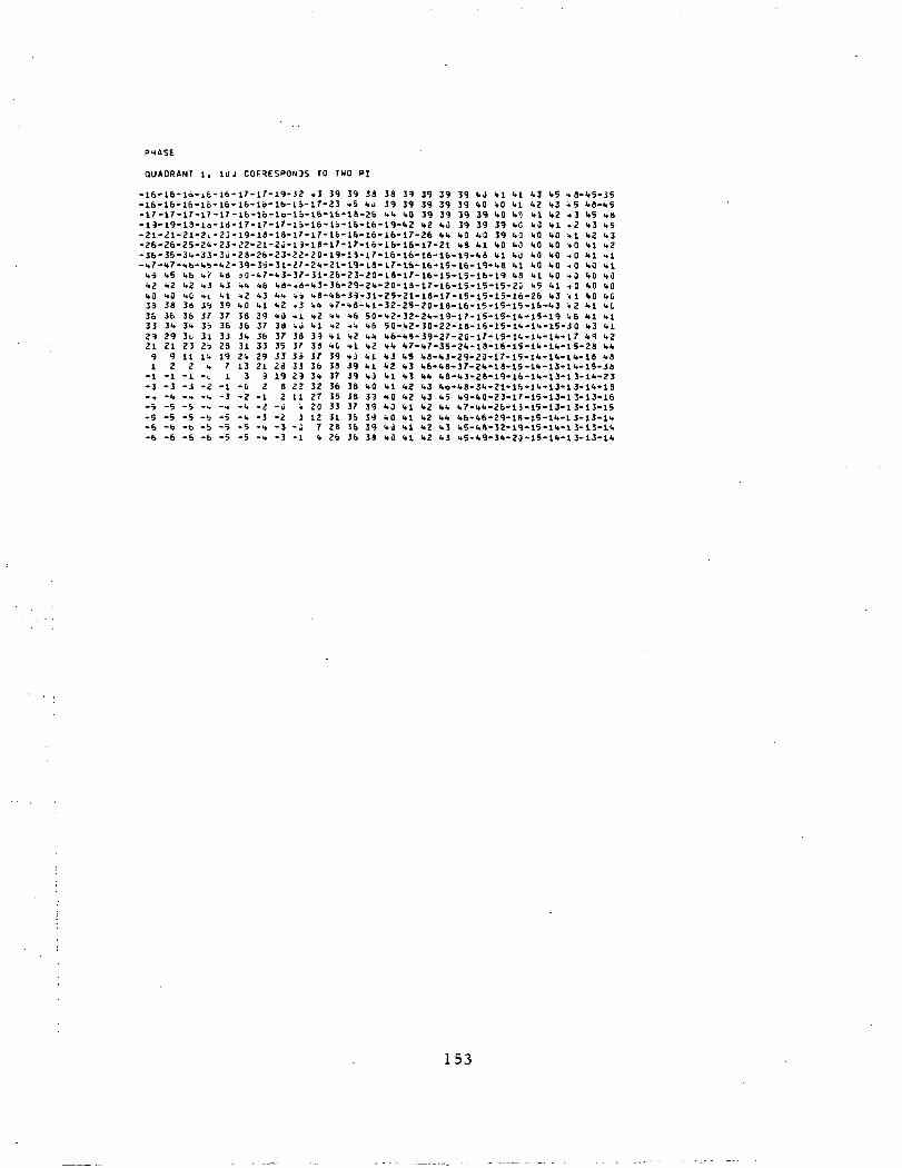
PH4SE
QUAORSNT 1, 10J COP^ESPONJS TO THO PI
-16-16--16-16--17-17--19-19--31-31--36-36--36-35--•7-1.7-
Ui 1.51.3 "21.0 1.033 3836 3633 31.39 3931 319 91 Z
-1 -1-3 -3
16-ifc-16-16-17-17-13-10-21-3i-35-3V3I.-33-Hfa-".!)-
1.6 <•/•1.3 43I.C »L
3d 3936 373U 3i3b 3133 2i11 li.
3 i.-1 -..
-16-17-17-
-i -5 -5 -.-5 -5 -5 -5-<-, -fa -b -b-6 -6 -5 -6 -5
17-•16-•16-•17--19-•33-•38-•39-
JO-41.
1.0S83631.3131.13
3-0-3-i.
-5-5
•19-33•16-15-
17-li-18-17-
33-33-31-37-1.3-37-1.3- d-
1.3••03837 3335 3733 353d 3319 JJ
8 333 11
-u <-3 3-3 -.j-3 -1
39 33-.5 i.j18-3615-16-15-16-17-14-1S-17-19-18-33-30-39-34-39-31-
-%8-i»l-<*& 50--'-. 1.6>.; i,u*l 1.3»a 1.139 1.139 1.038 1.038 3337 393o 3935 3936 38
33 3939 39ni. i*019-1.316-17-16-16-16-16-17-16-18-17-30-13-35-31-33-35-1.3-33-50-1.3-i. 6-1.3-i»l» 1.7-1.3 1.51.3 1.31.1 l.)1.1 1.3HO i>3UO 1.11.0 1.1WJ 1.11.0 1.1
39 3939 3939 391.3 ua36 1.U17-3116-16-16-15-16-15-17-16-18-17-30-18-31.-19-30-33-39-37-1.7-35-1.8-1.3-1.6-I.8-1.1. I.8-i»3 <»o-1.3 b51.3 1.1.1.3 1.1.1.3 1.31.3 U3
39 UJ39 1.039 3939 391.0 1.3-.3 1.119-1.816-19-15-16-15-15-15-15-16-15-17-15-18-16-30-17-ZI.-18-39-3-3-37-31.-U3-38-fca-Jt-I.9-1.0-1.7-I.1.-1.6-I.6-I.5-U5-n5-<»9-
1.1 <>11.0 1.11.0 1.039 1.039 UO1.0 1.01.1 1.01.8 1.119 1.8•15-3515-1615-1515-1U15-11.15-11.16-1517-1518-1519-1631-lb33-1736-1339-1S32-193I.-30
1.3 1.51.3 1.3>.! 1.31.0 1.11.0 1.01.0 1.01.0 UO1.0 1.01.1 1.01.5 1.1
•26 fc3•16-1.3•15-19•H.-IS-
•14-13-•H.-13-•1I.-13-•15-13-15-13-
'1S-1U-
• 8-<»5-351.5 US-US<3 I»S 1.8-.3 1.3 1.5»1 1.3 1.3-a 1.1 1.2•.o 1.1 -i-o i»a 1.1-J 1.0 1.0-o 1.0 1.0•t 1 «.0 I.C•*z 1.1 «.cU6 1.1 >.!30 1.3 1.117 1.9 1.315-28 1.1.11.-18 1.8
13-1U-2313-1U-1813-13-1613-13-1513-13-1413-13-Vl.
-15-1I.-13-13-H.
153
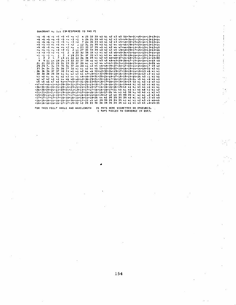
OUAQR4NT fc, luli C3H*FSPON3S 10 TWO PI
-6 -6 -6 -fc -5 -5 -5 -«. -> 4 25 35 J8 fcO fcl fc2 l>3 fc5 50-3fc-20-l5-lfc-l 3-13-lfc-6 -6 -6 -b -5 -5 -•. -3 -1 fc 26 3i 38 fcO fcl 1.2 1.3 fc5-fc9-3fc-20-15-lfc-l3-13-lfc-6 -6 -b -3 -5 -5 --. -3 -0 7 2i 36 39 fcO 1.1 fc2 1.3 fc5-fc8-32-19-15-lk-l3-13-lfc-5 -i. -5 -•. -5 -fc -3 -2 j 12 31 35 39 ".0 fcl 1.2 fcfc fc6-fc6-29-l S-15-lfc-l 3-13-11.-5 -5 -5 -i, -fc -fc -2 -u « 20 !3 37 39 »0 fcl fc2 fcfc fc7-fcfc-26-H-ll>-13-l 3-13-15... -fc -fc -, -3 -2 -1 2 11 27 35 38 39 *0 fc2 fc3 fc5 fc9-fcO-23-17-15-13-l 3-13-16-3 -3 -3 -2 - 1 -0 2 8 22 32 36 39 <.0 fcl fc2 fc3 fc6-fc8-3fc-21-16-lfc-13-l 3-lfc-18-1 -1 -1 -,. 1 3 •) 19 2i 3fc 37 39 fcj fcl fc3 fcfc fc8-fc3-28-19-16-lfc-13-l 3-lfc-231 2 2 fc 7 13 il 28 33 36 J6 39 fcl fc2 fc3 fc6-fc8-37-2fc-18-15-lfc-13-lfc-15-389 9 11 Ifc 19 2fc i9 33 35 37 39 «0 fcl fc3 fc5 fc8-fc3-29-?0-17-15-lfc-lfc-lfc-18 fc8
21 21 23 2S 28 31 33 35 37 38 fcC -.1 fc2 fcfc fc7-fc7-35-2fc-18-16-15-lfc-lfc-l 5-28 fcfc29 29 3* 3i 33 3fc 3o 37 J3 39 fcl fc2 fcfc fc6-fc8-39-27-20-17-15-lfc-lfc-lfc-l 7 1.9 fc233 3fc 3fc 3= 36 36 27 34 «a fcl »2 fcfc fc6 50-fc2-30-22-18-16-15-lfc-lfc-15-30 fc3 fcl
. 36 36 36 37 37 38 39 fcO fcl fc2 fcfc to 5U-fc2-32-2fc-19-17-15-15-lfc-15-19 fc6 fcl fcl38 38 38 39 39 fcli H fc2 fc 3 fcfc fc7-*S-fcl- 32-25-20-18-16-15-15-15-16-1.3 »2 fcl fcOfcO fcO fcu fcl fcl fc2 fc3 fcn »b fc8-fc6-39-3l-25-21-18-17-15-15-15-16-26 l»3 »1 fcO fclifc2 fc? fc2 fc3 fc3 fcfc fc6 fc8-.8-fc3-36-29-2fc-20-18-17-16-15-15-15-2u fcS fcl fcO fcO fcOfcS fc5 fc6 fc? fcii 50-fc7-fc3-3/-31-26-23-20-18-17-16-15-15-16-19 fcd fcl fcO fcO fcO fcO
-fc7-fc7-fc6-fcb-fc2-39-35-31-27-2fc-21-19-18-17-16-l6-15-16-19-fc8 fcl fcO fcO fcC fcO fcl-36-35-3fc-3i-JO-28-i6-23-22-20-19-18-17-16-16-16-16-19-fc8 fcl fcj fcO fcC fcO fcl fcl-26-26-25-2fc-23-22-21-2J-19-18-17-l7-16-16-16-17-21 fcS. fc l fcO fc] kO fcO fc0 fc l fc2-21-21-21-2k-20-19-ld-18-l7-17-l6-lb-16-16-17-26 fcfc fcO fcO 39 fcu fcO fcO -.1 fc2 fc3-19-19-lo-i3-lS-17-17-17-li-l6-16-16-16-19-fc2 fc2 fcO 39 39 39 fcC fcj fcl -.2 fc3 fc5-17-l7-17-17-17-16-16-16-li-16-16-18-26 fcfc fcO 39 39 39 39 fcO fct fcl fc2 -3 fcS fc8-lb-16-16-lt-16-16-16-16-lD-17-23 »5 fcO 39 39 39 39 39 fcO fcO fcl fc2 fc3 fcS fc8-fc5-16-16-16-16-16-17-17-19-32 fc3 39 39 38 38 39 39 39 39 fcO fcl fcl fc3 fcS t8-fcS-35
FOR THIS FltLT 4N5LE 4ND W A V E L E N G T H 26 R«YS HERE VIGNETTED OR 01SCUR£D,C RttTS FAILED TO CONVERGE IN SSRT.
154
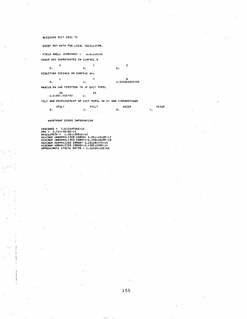
RECEIVER TEST CASE »1
CHIEF RAY DATA FOR LOCAL OSCILLATOR.
FIELD ANCLE (RADIANS) = J . Q g J J O J J O
CHIEF RAY COORDINATES ON SJ3FACE N
X Y Zo. a. o.
DIRECTION COSINES ON SURFAJE N-l
L I No. o. i.ooooojacE»oo
RADIUS RW AND POSITION TR 3F EXIT PUPIL
RW TR1.1120C;00£»03 0.
TILT »NO OISPLACEMENT OF EXIT PUPIL IN X- &NO f-OIRECTIONS
XT1LT TTILT XOISP YD ISP0. J. 0. 1.
MAVEFRONT ERROR INFORMATION
VARIANCE = 3.&3318706E-15RNS = <>.71iii*9476E-lSWAVELENGTH = 1.0611385l)£-iJ2HAXIMUM UNNORHALIZEO ERROR' 5.55111512E-17MINIMUM UNN3RMALIZEO ERROR=-3. JJQ-.'.SOSE-16MAXIMUM NORMALIZED ERROR: 5.2J128ZJ7E-15MININOH NORMALIZED ERROR=-Z.C93S1Z95E-1*APPROXIMATE STREHL RATIO = 1.00000JJO£*00
155
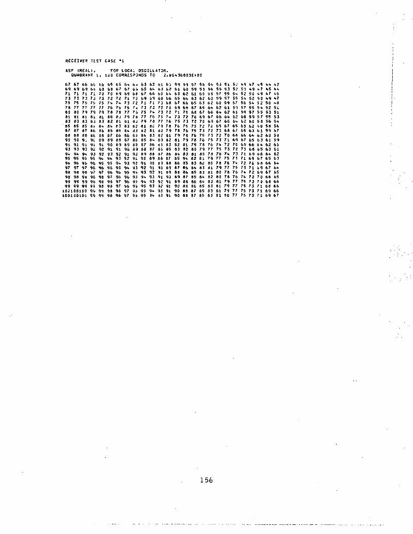
RECEIVER T£ST CAS£ *1
ASF (REAL), FOP LOCAL OSCILLATOR.QUADRANT 1, 100 CORRESPONDS TO 2. U0436003E*00
67 67 6669 69 6971 71 7173 73 7375 75 7578 77 7789 80 7961 81 6163 83 6365 65 8587 87 6788 86 8890 90 9.91 91 9193 93 9394 94 91.95 95 9596 96 9697 97 9798 98 9898 98 9899 99 9999 99 9910J100100100100100
6ibe,717 37b7779818i6s86Ob91919£93959696ft9696999995
66687073757779818381.86es8991929J9i.9596979898989999
656870727%7676608281.85878990919391.9596969798989896
656769727i.7b78ej81838566888991929391.95969697979898
61.6769?173757779818361.668769909192939*.959696<*69797
b.6i6875737,7578SJ83838586as899d9193939*9595959595
636567697173757779816361.656788899091929391.94959595
6261.66997173747678So818381.368788899091929393939414
6163656873727375777960828365858788a940919193929393
6'j6264666870727*7678798182838586878889899391919191
59616365676971737576787981828384856687688989909090
59606361.666870727375767879816283948566866786668888
57596163656768707373757678798081826384858586868787
56596062636567697072737576787989818283836484656585
5456S860626466676970727375767778798081818283838383
53555759606264666769707373747576777679806061818181
51535557596162646667687071727374757677767879797990
5J53
5-555759616264
65676869707273717475767677777777
4950S354565759606263656667687571717273747475757575
47495052545557596062636465666669697C71727273737373
45474950525 4555758<JO616263646566676869697070717171
44 4245 441.7 4649 47SO 4852 5C53 5155 5356 5456 5659 5760 5861 5962 6063 6164 6265 6366 6467 6467 6566 6568 6668 6669 6669 67
156
Q U A D R A N T 2, l i JO C O R R E S P O N D S TO 2. t i t U36003£»l)0
<.2i»i.»51.71.85051S3S<.5b575t)596 j6162635<.6".656566666667
i.51.7".9505253555b5859606162636<i656667676868686969
1.71.95052Si.Si5758606162636u6i>66fc76869697C70717171
<«ySi52
5-555/S'a61626361.6i63bb5Sb97l7172717:737373
eo52Si.9057596.62116$fo67Id707171727371.714757575'/•>
525".55S759bl626»65o768697072737371.75767677777777
53555759flt2ei.60f7687J7172737".7576117373797-379e:.
55S?596062ait66676970727371.75767770798J8081818181
5 3
itbub25«6io7697J7273757i777879JOHI11S23J8]3]dj
586052636567b97072737576787980SI82838381.di.058585
59SIS36567-,87*72737576787980818213
3-853596168757
6u626".09
68707273757578799132333U158->861788383838
59Si6365676971737576787981328381.85868733898990909J
606261.6668707271.7678798182838586878899899091919191
61636568707273757779808233358687338993919192929395
626fc6669717371.76788C81833U363738899091929393939«.91.
636567697173757779818281.85878889909192939*.91.959595
61.6663707271.7678808283858688899091929391.9595969696
6U67697173757779818381.8687899u91929391.959696969797
656769727U76781081331536883991929391.95969697979898
6561707271.7678808281.8587899091959U9596969793939393
6663707375777981838=.8683899192939U9596979891989999
6668717375777981838586889091929395969697989899
S6 6769 6971 71f3 7375 7577 7779 8031 3113 8335 8587 8788 88TO 9091 91•)3 93)u 91.95 9516 9697 9798 9898 9899 9999 99
9910 0100991: oioc
157
QUADRANT 3, 130 CORRESPONDS TO 2. J0<.3fegi)3E»00
67 69 7167 69 716b 69 7166 66 7166 68 7C65 68 7C65 67 696. 67 696* 66 6863 65 6762 61. 6661 63 65bj 62 6U59 61 6358 60 6257 59 6156 56 605". 55 5853 55 5751 53 555J 52 5".1.3 50 521.7 »9 5:<t5 n7 1.9
n737;7j7372727;7u69ol6b6t666U636<-6 159575b5-.52Si
757575757571,7 it737271717u696766656362605957565452
7a7777777776767571.737372706969676561.626159575551.
t» •
»c*
o
797979787877767574737271?Ci5t7666t12615vi5.7SS
8161816181808ii797877767571,737270o967666U62605957
6183838}8382HI91rtj7978777i7i73727 j69b703
04
62oJ56
d58585658<t81.83838281811797876757372706967656)6263
3787876686958591.83929180797876757372706967556361
888848868887839=>351".931)29179/37i75737270696b&<.62
9J9090939969888786858<>83528179787675737169676563
91919191919089898897868583828179787671.7270666661.
939393929291919089688786858382837977757372736865
9k91.91.9J93939291906988B766»!.838180787671,73716966
9595959591.91.9392919069886785ei.826179777573716967
96969696959591.93929190898886658382aa76767»727068
979797969696959»9392919089676661,6361797775737169
969698979796969591.93929199686685838180767671,7269
99989998999796969591.93919069876581.82607d7671.727g
999H999998989796959»93929189886661.8381797775737D
991J0100991 j 0100991J010C999898979696959392919086666583817977757371
99 9999 9998 9698 9697 9796 9695 9591. 91.93 9391 9190 9086 8887 8795 8583 6391 8179 SO77 7775 7573 7371 71
-.i. 1.5 1.7 -9 5J 52 53 55 ?6 58 59 60 61 62 63 bk 65 66 67 67 66 68 68 69 691.2 1.1. 1.5 -1 45 50 51 53 5-. 56 57 59 59 60 61 62 63 66 6". 65 65 66 66 66 67
158
QUADRANT i>, 100 CORRESPONDS TO 2.Olo3bOJ3E»OG
lOOlOOlOli1001001001001001009999989897969590939190aa8785338180737573716967
9999969897969590939190888735838180777573716967
999998989796959093919C838785838179777573716966
94
9999989b9796969593929191aa368543817977757371-6866
INTERVAL *
99999994989897969590939291896836so8381797775737u68661
98989898989796969590939190498785808280737670•72706865
9893989797969695909392916988666583ei8378767o72696765
9797979696969590939291908987868083817977757371696760
.036295056
959693
9595909392919J8988453543928078757«727J6)556*-02
9595959590909392919049883785808281797775737169676563
909090939393929190696887168013118u787670737169666062
4393939292919190198637353533323d79777573727066656361
NU1BER
9191919191906969888786858382817978767-.72706666606261)
909090903939686786858V836281797876757371696765636159
683«86686687866665SO63626179767675737270686660626-153
INTERVALS
8787878686653580836261807978767573727068676563615957=
65858585608063638281807973767573727C6967656362605656
51
3]83138333328141307973777675737270696766606260585650SUM
6161616181806979787776757073727069676660626u59575553=
80807979797878777675707372717068676660626159575553510.
73777777777676757".73737270696967656062615957555052s:
75757575757070717271717066676665636260595756So525008
73737373737272717069696866656063626C5957555052500907
71 69 6771 69 677 1 69 6671 63 6670 63 667 0 68 65&9 67 6569 67 6063 66 6057 65 6366 60 6265 63 6160 62 6033 61 5932 60 58•il 59 5750 58 5658 56 505 7 55 5355 S3 5150 52 5052 SO 08SO 09 07,9 07 05+ 1 05 00-.5 Oo 02
159
RECEIVER TiST CASE •!
AST ( IMAGINARY) ,FOf. LOCAL OSCILLATOR.QUADRANT 1, 103 CORRESPDNOS TO 2.-.2048796E-09
-7l-71-7C-7i-69-b8-t 7-65-bJ-bl-57-53-5i)-45-42-38-35-30-22-l«-14 -9 -5 -3 -1 0-7l-71-71-7i,-/.i-o9-fc7-&6-6..-bl-57-53-49-45-'>l-38-34-29-21-17-13 -» -4 -2 -0 1-7l-71-71-7,.-7D-b9-67-65-:>3-bl-57-53-49-44-41-37-33-2B-2:>-16-ll -6 - 2 - 0 2 3-70-70-7 J-7,,-69-68-&7-&S-63-60-5&-52-48-43-39-36-32-27-19-14 -9 -I. -0 2 4 5-67-b7-bb-6o-t9-b4-63-61-39-56-52-48-4..-39-3b-32-28-23-15-10 -5 0 <• 6 8 9-61-61-61-6.-e.J-59-E7-55-i3-S>l-<.7-43-39-34-30-27-23-17 -9 - 5 - 0 5 9 11 13 14-57-S7-56-5b-55-54-E3-51-4j-46-42-38-34-29-26-22-18-l3 -5 0 5 10 1* 16 17 18-52-52-S2-5;:-E.l-50-49-47-45-42-38-34-30-25-21-18-14 - 8 - 0 S 9 15 19 20 21 22-43-43-43-'.2-42-41-40-38-3-I-33-29-25-21-16-13 -9 -5 -0 8 13 17 23 27 28 29 3t-37-37-37-3;-3c.-3fa-34-32-3u-2B-24-2u-16-ll -7 -I. 0 5 1* 18 23 28 32 33 3". 35-34-34-34-33-J3-32-31-29-27-24-20-16-12 -7 - 3 - 0 4 9 18 22 27 32 36 37 38 38-3J-30-3.-31-Z9-29-27-25-23-21-17-12 -8 - 4 - 0 3 7 13 21 26 30 36 39 «1 1.1 42-27-27-27-2t-26-25-24-22-2j-17-l3 - 9 - 5 0 4 7 11 16 25 29 3d 39 »3 41. 1.5 1.5-22-22-22-21-21-20-19-17-15-12 -8 -4 -u 58 13 16 21 30 31. 39 44 1.6 *9 ".9 50-1S-18-18-1/-17-16-15-13-11 -8 -". 3 4 9 12 16 2i 25 3fc 38 1.3 1.8 52 33 53 53-1*-1'.-13-13-13-12-11 - 9 - 7 - 4 C I. 9 13 17 20 ?* 29 38 1.2 *7 52 56 57 57 57-9 -9 -9 -% -B -8 -6 -U - 3 - 0 -. 8 12 17 21 2fc 28 33 1.2 ".6 51 56 60 61 61 61-7 -7 -6 -f. -6 -5 -•. -2 -J 3 7 11 15 20 23 27 30 36 1.5 *9 53 59 63 63 6b 63-5 -5 -5 -". -u - 3 - 2 - 0 2 i. 9 13 17 22 25 29 32 38 fc7 51 55 61 65 oS 66 65-3 -3 -3 -Z -2 -1 -J 2 4 6 11 15 19 2". 27 31 34 40 49 53 57 63 67 67 67 67-2 -2 -1 -1 -1 -u 1 3 5 8 12 16 20 25 29 32 36 41 50 54 59 64 68 69 69 68-1 -1 -1 -w -i. 1 2 4 i 8 13 17 21 26 29 33 36 42 51 55 60 65 69 '0 70 69-J -C -: -„ j 1 2 4 i 9 13 17 21 26 35 33 37 »2 52 56 60 66 70 70 7-j ? i-J -6 -; L I 1 3 5 > 9 13 15 22 27 30 31. 37 43 52 56 61 66 '70 7i 71 7C- 0 - 0 u t 1 2 3 i) 7 9 14 18 22 27 30 34 37 43 52 57 61 67 70 71 71 71
160
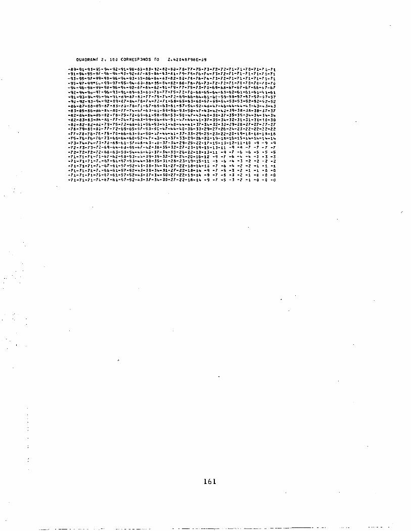
QUADRANT 2, 10J CORRESPONDS TO 2. >,20l.879eE-a9
-89-91-93-95.-9«.-92-91-90-8J-83-S2-82-80-78-77-75-73-72-72-71-71-70-71-71-71-91-9I.-95-97-96-9i.-93-92-8/-8S-8i.-S3-ai-79-79-7b-7»-73-72-7 1-71-71-71-7 1-71.93- 95-97-99-98-95-91,-93- S9-86-8I.-* 3-8 2-8 0- 7«-76-7l»-7 3-72-71-71-71-71-7 1-71-9S-97-99*Gi,-99-97-95-9<.-i9-86-35-8<.-82-80-78-76-73-72-7 2-71-70-7 0-7 0-70-70-9I.-96-911-99-9U-96-91.-92-87-8".-82-51-79-77-75-73-70-69-6S-67-67-67-66-J 7-67-92-9i»-9b-97-9&-93-91-69-a3-bO-76-77-75-72-70-&8-6S-6i.-63-62-bl-&l-61-'bl-bl-91-93-9".-9i-9it-91-S9-87-8J-77-75-7i.-72-69-66-6<.-61-6C-59-58-S7-5 7-57-j 7-57-9J-92-93-9W-92-89-67-8".-7 8-7 i.-72-71-68-65-53-60-67-55-5".-53-53-52-52-1j 2-52-86-97-88-89-87-8 3-f 0-78-71-67-65-63-6 l-57-Sl.-S2-<.S-l»7-l.6-»l.-l.»-l. 3-1.3-.. 3-1.3-83-85-86-«b-8'.-80-F7-7'.-i7-63-ol-S9-56-53-50-'»7-<.3-'»2-i.J-39-38-J8-38-J7-37-«2-8i»-8'.-8S-82-78-7S-72-55-61-58-55-53-50-'»7-»3-<>0-38-37-35-35-3".-3't-!<.-3'«-82-83-83-81.-91-77-7i.-70-b3-59-56-ii.-5l-i. 7-1.i.-(.l-37-35-3ii-32-31-31-31-1 0-30-8i)-82-e2-»i- 79-75-72-68-61-56-5 3-51-i.S-". <.-<.!- 37-31.-32-3 J-29-28-27-27-J 7-27-78-79-80-80-77-72-69-65-57-5 3-5C-1.7-1.I.-1.0-36-J3-29-27-26-2I.-23-22-22-2 2-22-77-78-78-76- 75- 70-66-63-5-.-50-+7-<» <.-»!- 37- 33-29-25-23- 22-20-19-18-18-18-18-75-76-76-76-73-68-6l»-6(l-5>-i.7-»3-»l-37-33-29-26-22-V9-18-l6-15-ll.-ll.-li.-ll,-73-7l»-7i.-73-70-65-fcl-S7-i.9-".3--.0-37-3l»-29-25-22-17-15-13-12-ll-10 -9 -9 -9-72-73-73-72-69-6l.-tJ-55-'.7-i,2-38-35-32-27-23-19-15-13-H -9 -9 -7 -7 -7 -7-72-72-72-72-6S-63-5-S-5'«-'.i-<.u-37-3i.-30-26-22-lB-13-ll -9 -7 -6 -6 -5 -5 -5-71-7l-7l-71-b7-62-58-53--<-39-35-32-29-2i.-20-16-12 -9 -7 -6 -«. -l» -3 -3 -3-71-71-71-7,-67-61-57-53-I.1.-38-35-31-28-23-19-15-11 -8 -6 -•» -3 -2 -2 -2 -2-71-71-71-7i.-67-61-57-52-1«J-38-3l.-31-27-22-18-l<.-ia -7 -6 -«. -2 -2 -1 -1 -1-71-71-7l-7L-66-6l-57-52-»3-38-3i.-31-27-22-18-H. -9 -7 -5 -3 -2 -1 -1 -0 -0-71-71-71-70-67-61-57-52-1.J-J7-31.-JO-27-22-19-1I. -9 -7 -5 -3 -2 -1 -0 -0 -0-71-71-7l-7l,-e7-61-57-52-'.3-37-3<,-30-27-22-18-ll. -9 -7 -5 -3 -2 -1 -0 -0 -0
161
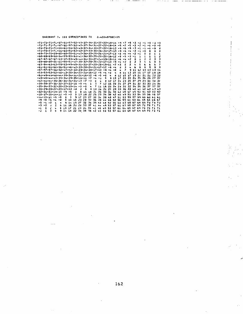
Q U A D R A N T 3, 100 (TORRES" DUDS TO 2. kZOk8798E>09
-71-7l-71-7l-67-61-57-53-kl-;i7-Jk-30-27-23-18-lk -9 -7 -5 -3 -3 -1 -0 -0 -0-71-71-7l-7i,-67-&l-57-53-'.3-37-3k-3u-27-22-18-lk -9 -7 -5 -3 -Z -1 -C -0 -0-70-71-71-7C-fc6-61-56-52-k3-37-l<.-.JO-27-22-l8-13 -9 -6 -5 -3 -1 -I -0 -0 0•7a-70-7D-7i-tb-60-5o-S3-k2-37-33-30-3b-31-17-13•69-70-7C-69-65-60-55-51-»3-36-33-39-36-21-17-13•68-69-&9-&8-6H-59-55-5u-kl-36- 33-29-25-20- 16-12.67-67-67-67-fc3-»7-53-k9--.u-3k-Jl-27-3<-19-15-ll•65-b6-65-6S.-tl -55-51 -k7-33- 32-29-25-22- 17-13 -9•63-6k-63-63-f9-53-k9-k5-3o-3G-37-23-30-15-ll -7• fc1— fel»fi1*fef-»^f»*Sl»I*f»»U?»'i3»?fl»?**— 7 l » 1 7 » i > «• A *L' D l O 4 ~ D l ™ D L 5 O ? l * « O ~ H t ™ J J w C O C » * ~ c t l r " l c "0 "*»
•57-S7-57-ib-52-k7-fc2-38-29-2k-20-17-13 -8 -k -0•5i-53-53-52-k»-»3-J8-3k-2;-2iJ-16-12 -9 -k -0 k•50-k9-k^-k8-kk-39-3k-36-21-16-13 -8 - 5 - 0 k 8•k5-kS-k-.-k3-39-3k-Z9-25-li-ll -7 -k -J 5 9 13•k2-«.l-fcl-39-36-30-26-21-13 - 7 - 3 0 k 8 13 17•38-38-37-36-32-27-22-18 -9 -k 0 3 7 12 16 20•35-3k-33-33-3S-33-18-lk -i -0 k 7 11 16 20 2k•30-29-28-27-23-17-13 -8 3 5 9 13 16 21 25 2922-21-20-19-15 -9 -5 0 8 Ik 18 21 25 30 3k 38
-9-8-8-6-k-3
0k8
1217212k2833k2
-6-6-5-k-2
0
711152023273036k5
-k-k-3-2
02
913172335293238k7
-3-3-1
02k
1115192k27313k
k9
-1-1
u135
12162025293236kl50
-00I2k6
13173126293336k251
0012k6
13172126303337<>252
011356
13182227303k37k352
012357
Ik182227Jf3k37k352
-18-17-16-lh-lO -5 -0 5 13 18 22 2b 29 3k 38 <*2 <«6 ".9 51 53 Sk 55 56 S6 57-lk-13-11 - 9 - 5 0 5 9 17 23 27 30 3<. 39 »3 *7 51 53 55 57 59 60 60 61 61-9 -8 -6 -i. -0 5 10 15 33 28 32 36 19 <•* <>8 52 56 59 61 63 6U 65 66 66 67-5 -<• -2 I <• 9 lu 19 27 32 36 39 it] <>8 52 56 60 63 65 67 68 69 70 70 73- 3 - 2 u 2 6 11 16 20 29 33 37 <•! <«, <*9 53 57 61 63 65 67 69 70 70 7 1 71-1 0 i fc 8 13 17 21 39 3k 38 m k5 k9 53 57 61 6k 65 67 69 70 70 71 71-J 1 3 5 9 Ik 18 22 30 35 18 k2 k5 50 53 57 61 63 65 67 61 69 70 70 71
162
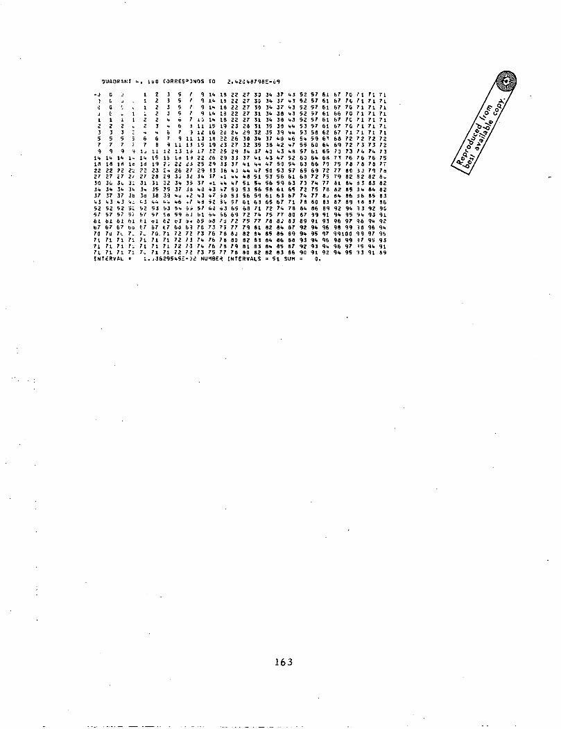
i., luO CORPES'DNOS 10 2.1.2S 1.879BE-J9
-J 0J C.C 0j CI 1a 23 35 57 79 9
1". li.IS 1822 2237 2730 3li34 3".37 371.3 ".352 5257 5761 bl67 6770 7U71 7171 7171 71
jut.
w1
23579
!<•1*?2c73u31.371,3525761677i717171
4
11t
;;
;••j
i-162;.-2/3;3".3bi,;Si5ihibb7.717i71
INTERVAL =
111122
^67ij11.li7227311*3d1.35257fclt77_
71717_
1.
222223<•69
1115192328313538<,!>
5357ol6770.717171
3333>»*»
679
1213
?;2 *29321539"-«53;a62t771717171
5555b6791113la2226303<*37<*u<>65»59b36672727272
;36295i.5£
/rt77i9
11111319iJ27113533-.2,75 joJ34
6)72737372-32
9999
1 j111213IS172225293<>37<>0<<31,8576165707371.71.73
11.11.I*1"4
I*
151610192226291317«li*3".7526061.087376767675
1813181818192022i32529!336-.1-."..750
5'-.o3=>6'a7578787877
NUMBER
2222222222232".2627293337I.Jti.1.7SO5357656972778J837978
2727272727282930323i>371.11.1.1.851S356616872757982828180
3339303131313231.35371.1"."»1.7515*5659637171,7781a i.838382
INTERVALS
31,31.3k3U31.35353738i>31,31,7505356586165727578828581.81.823
373737383839391,01.21.31.75053565961636771.778J81.86868583
1.3<t31,3t>31,3l,1,1,1,61.71,852BI.5761636567717880838789888786
51 SUM
5252525252S3535".55576]6365687J7271.7881.87899291.939290=
5757575757575859606151.66697271.75778086999191.9591.93910.
61616161616162616<.656870727577788j838991939697<959i.92
67676766676767686970?•»757779818281.879291.9698
707t70707C70717272737678808281.85868991.959799
99100989691.
999795
71717171717171727371,75783J32S3Ji.1618139".96389997>S13
71 7171 7171 7171 7171 7171 7171 7172 7273 7271. 7376 7578 7779 7b82 8U83 8281, 8285 8387 8692 9093 9191, 9296 9i>97 9595 939fc 9191 89
163
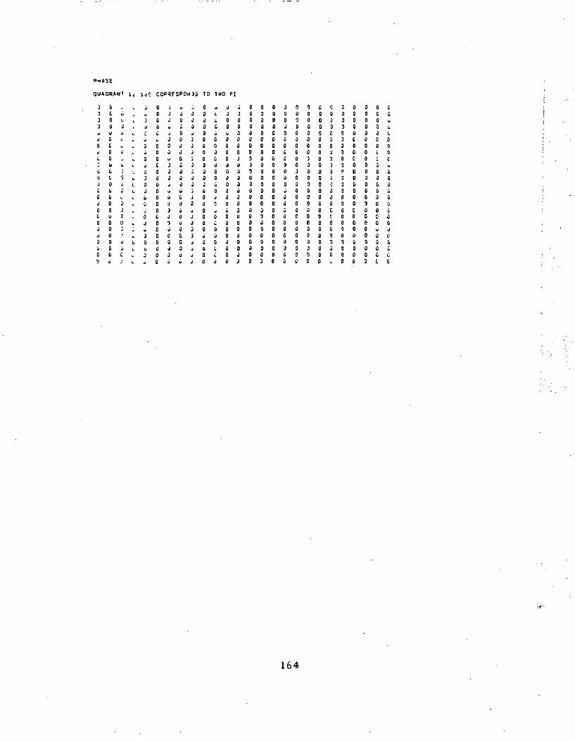
PHASE
3 Ii .3 C b3 II u•3 II 0u U JJ G K0 C -n B 0i. (J: u bo c ;o c Qj o -jC ti i3 0 LJ 0 30 0 3C U 3g o u3 o :J 0 .'3 D uii C 3C 0 C
0 D
IJC
jw
3U;u
3J3j$3
Dj
u0y
3jy
J
0u3
CO
00C00b
C00c33b0333C3C0330
iP*F5HU
J »
J hi
J 0* V
j 3J 33 JJ Ju 0J 0J 03 3» 0u uu ii3 93 uj 00 uj 33 C3 0J 3J 0
NJi 13 IN
- 0 b
3 0 1 .J J L
3 0 C.j 3 J3 0 CJ 0 3j 3 jj 0 C3 0 03 3 DJ 3 3J 3 J3 U 3j 0 d3 3 0J O *J 0 0J O . ;3 0 33 J 0j a cJ U Ij 3 i
10 H
JJ
03uJ0I]0J0<J3330it
3330033
I
j3333300JJ33jii3330a0a00>)
003033003J00300033000030
3 03 03 00 0g o0 00 00 00 09 00 33 00 03 00 00 0i 33 03 0g o3 0o o3 03 0
:
03J003uD90uay3303330033
ao-333333303333003C30003n
033333030330333g30003a3g
3300g3000000000000000030
0033303J333u.j333Cr
0C333C
3331g33•]3gP33033000g0a0g
0 3C 00 30 00 3I 30 00 0C 00 00 00 3C 00 03 30 30 30 00 00 00 0ii 03 33 0
3C333C0ccJ1)3C330000u3C3C
CQ
g
M
I
330Cu
03Db
3au300C(ibC
164
QUADRANT <., 10 J CORRESPONDS TO TMQ PI
li0300004;li
u000jc000
300a00
000000000
00c000000
000000
uc0Gf0V,
uI-
su030t
u
u0fu
Ja3000
,.I0I,t
LcIcL
IcI,LI„t_
LwiL
ty
t0
u00Q3Q00j
000al)0ugJ30a3a
ii00300g00U
0cI)3003Q0
000000
J03033330
00033j3aJj03JQ0
0u3Cj0000
Jd00g0000
300003
3 0 03 a :3 0 0j o a3 0 03 0 33 0 3j 0 il3 0 3O ft r
U w
3 3 Cu 0 0
3 0 C3 0 03 0 03 0 03 0 01 0 03 0 C
3 0 ii3 0 0
3 3 03 0 0a o o} 3 0
00003i)000
a00000g30
00o000
03030003a0agu0300000000g00
00000000a000000000000000a3
9o30g30a00aI03030000300000
0 00 30 30 00 J0 <l0 30 00 U
0 i)0 30 u0 30 00 00 3o a0 0O iiU
0 00 u0 0o a0 00 3
900000901]
a00003000
000a00
0aa00o090
09003U000
ag000g
0 00 u0 U0 0c -.0 J0 03 J0 J
0 *0 ;a }0 J0 io a0 0a ia La -U
0 30 j0 30 J0 00 J
093393999
0909903a9
099993
00000000Q
0000c0000
000000
00ag90090
a0gg03390
00g000
(l0i.0c030i)
000a0cc00
c00030
G3003tUu0b
u
3u0c0£dU
3110u
U,.
165
RECEIVER UST CAS- •!
DETECTOR COMPUTATIONS.
DETECTOR NO. = 1RECEIVED SIGNAL BEAN IS SHIFTED X = 0. AND Y s a,WITH PESFECT TO CENTER OF DETECTOR.
LOCAL OSCILLtTOR flEAH IS SHIFTED X = C. AND T = 0.WITH RESPECT TO CEf.TER OF OETECTOR.
CIRCULAR OLTECTOR CIAMET;? = 2.:72J9091E-01
SIGNAL "OHjo = I.59fc7bb3i».'»LOCAL OSCILLATOR POWER - 1.Z85JU27E-01CROSS PRODUCT POWER = 3.iJZ58Z6E+JiPHASE MATrn iFFICIEfCf = 3.595U11E-01 I -.016 D3 )AVERAGE PHASz SHIFT (RAOIA1S) = Z.6263Z01E-01OPTICAL TRANSHISSIOh' = 9. ?581079E-01 < -.106 0? )FOCUSING EFFICIENCY - 7.b»31/a6E-Jl < -1.167 OB )NON-HETERCOYHt DETECTION EFFICIENCY = 7.<t$8Z9u3E-31 C -1.371. 08 >L.O. ILLUMINATION EFFICHN;Y = 8.a9iii)5i»E-oi ( -.8i» 08 )M A V I H U M 4ia t NM« G A I N = i, 38t>a915E»3S ( 93.777 04 )R E C E I V E R I F F I C I H N C Y TO I.F. = ». 72J1.376E-L1 ( -3.260 OB I
166

APPENDIX D
SIMP BIT l td l = sJ .975,i .62t , Md> = C . , . . , HAidl - 0.,!.. IFUGKl l = 0,0,= -!...-•>. M C I ) = i.13, <L!N\M1I = ;.. -9.I.-356957-'.,
= '.., -102^. , }., 52 .0)152, 3-..0868, 3')., -105.120".'., -161.5S6-.,= !•„., lLb3. IB iS i ) , bod.2130-., 3., -105.120<>H, -161.569<,, 0., 0. ,
T 3 d > = C., -51".., -32.1, -2., -910., C., 0.. -193., -2..0.,TSd l ) - -100.3 , C., u. , -2., -312., -193., -2..J., -100.3, J.<X l U S d l = :•, -1., -I., -«.;iiji2, i»*-l., -l,.1.0062, •»•-!.,Xl l lSd^ls -^ . i J J62, -1., -I., -«.l!)062, 3*-l.,$ < A P A ( 2 ) = ..,P Z E R O d l = -1.-6, 1.-3,Z O M E G A = 1.-J25,
167
LACONA - LASER C3NHUNICATOR ANALYSIS PROGRAM
• • • • » PAGOS CORPORATION .....
RECEIVER TEST CASE *2
RECEIVED SIGNAL OPTICAL 3ATA.
N -12 BETAO 5.397SOQJOE»01 H 0.
M 1 XLINV 0. HAS 0.
P?£RO -l.Oi.OtiOOOCE-06
IFLG1 0
SURFACE PARAMETERS
SURF. CURVATURENO. RHOS
1 0. 0.2 -9.72762b5E--J'.-5.14JjiiuOE*023 0. -3.21J3JOit 1.69388i.9E-02-2.iiuOJOu5 2.933bS69E-.2-9.Ui:.)ObOE»G26 0. 0.7 0. 0.8 0. -1.9J9 -9.5128978E-C3-2.0u-JuOOE*00
10 -b.l862567t-il 0.11 0. - J . J O12 0. 0.
SURFACE SKAPA
2 C.
SEPARATION INDEX OBSCURATION DATA VIGNETTING DATAT5 XNUS BETAPX BETAPT BETAS* BETAS*
0.0.0.0.C.0.0.0.0.0.0.C.
ASPHERIC COEFFICIENTSBETA GAHMA DELTA EPSILON
0. 0. 0.
OE»02OE»01O E » 0 3O E 4 - 0 2
O E » 0 2O E » 0 0
OE»02
i . t ooooo- i . tooooo-1 .100GOO-<>.cao62a- l . C O O O O O- l . C O O C O O- l . C O O O O O-1.000003-*..(, 00620- i . cooaoa- l . C O O O O O- i .coajoo
a.0.3.0.u.j.0.d.0.0.0.0.
0.0.0.C.0.0.C.0.u.0.0.0.
0.0.0.0.0.0.0.0.0.0.0.0.
ALPHA
FIELD ANGLE - J.
168
LOCAL OSCILLATOR CPTICA>. O A T A .
N -8 3i.TAj 2.12103... JtHJL H Q.
H 13 XLINV -9."-j569i/jE-Ji. MA3 0.
PZJRO 1 . 0 . O C O O O J E - O J
IFLSl 0
SURFACE P A R A M E T E R S
SURF.NO.
13I".151617181929
0.9.1.0.-9.-6.0.C.
CURVATURE SEPARATION?HOS T3
0.<.05&957£-'J<.-2.JCjJgOOE»l!0*-935287E-C3~3.92^jyjJE*j2
~1.93JjuCOE*0251tb978E~03~2.0GjjJOOE*jG1892908E-J3 0.
~1.0t3jwuOE + lj20.
INDEX OBSCURATION
-1-k-1-1-<t-1-1-1
XMUS 9ETAPX
.000000 •}.
.000620 0.
.cuoooo a.
.000000 0.
.C00620 0.
.toOuOa o.
.tooooa o.
.CJJOOO 0.
00c0c000
OATA VIGNETTING OATABiTAPT 3ETASX BETAST
•j. 0.0. 0.C. 0.C. 0.C. 0.a. o.o. o.a. o.
FIELD ANGLE = a.
NXT = JS NDET = 1 NFRS = Z6OELFS = 0. ZOMEGA = 1.62SOCOOOE»00 VLAMOA - 1.i611385CE-03
DETECTOR OATA.
OETECTOR NO. 1 IOETEC = 1 J 0 0 0
169
FiTA
P4RAXIAL RAY TRACE - RECEIVED SIGN4L OPTICS.
ALPHAb , 7 9 7 & . L O L E * u it . 397b i .L - - J E » D 12 . 2 7 3 ? ? f a 7 5 £ - l Z
- 3 . 3 7 t f c l Z 2 6 c » u t- 3 . 5 l 9 v 7 2 d 4 £ » . - C
B . 5 C W ; 5 i63E»u lA c t - J ' ^ ^ S ' ^ u L
6.5<.*3 J 3 b 3 E » JL1. 1L5'.3528E*.11..9i ,32115E>Cl1..9C3?115t*Jlt i . c ) f c C ; ' ^ 7 0 3 E - J l
).-1 .05J09728E-01-1.0iOC97J8E-01-2.96567218E-01
1. 321253<.6E-021. 3212531. f>E-021.3'1253C6£*021. 32l253k6E-02
-3.0232941.9E-01-1 .98720J22E-02-9 .9172J322E-02- 9 . 9 6 7 2 J u 2 2 E - 0 2
C.0.9.5229272SE»00l .QH7ofc7tE*011.9>>li>3iie9E»tl
-2.6375BS72E»02• ? A 1 7 Q A C 7 ? F * f l 9™c« O Jf SO 7f ct. + vc
-2.83758572E»C2-3.".61i.9093E»02-3.1.1371125E»02-3.*1371125E»02-1.85»2i.06a£»01
1.85270959E-021.85Z70959E-021.85270959E-J25.93^9566CE-01
-3.232669I.6E-01-3.232669i»bE-31•3»232669U6E*01-3.232669k6E-01
9.557<.17l.5E»aO3.21863129E»003.21863129E»JG3.21863129E»00
P A ^ A X I A L ENT-!ANC£ PL'PIL PaSITION TO) = -0. TEXIT= -1. t
INVERSE OPJ fcCT OISTtNCE XLINV = 1.
FOCAL LtNGl* = S.U'.«173<E»i)Z RACK FOCAL. LENGTH = -1.09171853E»S2
TS(N- l ) = -i. 09171S53E»J2 Ft = 5. <.C»l.l75i.E» J2
170
P1RAXIAL RA» TRACE - LOCAL OSCILLATOR OPTICS.
P E T 3 R A L P H A A2 .62Ku. . j i ,E» Jl }. 0. 1.81533766E-012.621. ; ; . , JE»JC 7.39722i95E-03 0. • 3.81533766E-012 . 6 2 U b 9 8 J i . E » J C -<..3a9ai631E-03 1.90737319E-01 .80677257E-a 19.0<»2u3e'.8t-Jl -<..339J1631E-03 l.i»9416222E»02 .8 J677257E-015 . ^ 1 2 o 5 C J 7 E - 0 £ -5.C1958J29E-03 2.22986933E»02 - .931S3915E*J0
2 -i.i)lit59053E-aJ 2.19896627E»02 - .89768283E»0 01 -5.011.59J53E-03 2.9S590 392E»Ot - .89768283E*0 0
P A R A X I A L E N T R A N C E PUPIL P O S I T I O N T ( O I = - 0 . T E X I T = -1.15876385E»02
INVERSE OBJECT D I S T A N C E X L I M V = -9 . i ,OSo9S70e-C»
FOCAL L E N G J H = 5. 2267".7.1 J i » 0 2 1ACK FOCAL L E N G T H = -1. 07913«<>aE»01
T S ( N - l ) = -l .o85*9893E»ii2 FL = -3.6166<.382E»02
171
RECEIVE* TiST CASE '2
CHIEF RAY DATA FOR RECEIVED SIINAL.
FIELD AMGLL IKAOIANSI « b.uujiujoc
CHIEF RAY COORDINATES ON SJRFACE N
X T Z0. J. C.
OI-tECTIOM CDSINES ON SURFi:j N-l
L M No. _•. - i .oooooa; i iE»oo
<ooius RH AND POSITION T? ar EXIT PUPIL
*w TR-3.11ld9259E»Lj -1.^606096JE«02
TILT AND DI5°LACE1£NT OF £<IT PUPIL IN »- AND T-OIRECTIONS
XTUT YTILT XOISP YDISP
.HAVEFRONT ERROR INFORMATION
VARIANCE = Z.J1695fc38£-3Z
WAVELENGTH = l.ublli65JE- J£MAXIMUM UNNORMALIZET ERRO-?= it.MINIMUM UNN3PMALI2tD ERRO^ = - a . 1 195 93".l£-0lMAXIMUM NORMALIZED FRROR= J.MINIMUM NORMALIZED f RROR=- . b517753mi- 3cAPPROXIMATt STREHL fATIO = 9. 5U081 996E-C1
172
RECEIVER TEST CASE «2
CHIEF PAY DATA FOR LOCAL DSCILLATOR.
FIELD ANGLi. (KAOIAFSI = u . jO J.J 0000
CHIEF RAT COOROINATIS ON SJRFACE N
X tI). J.
DIRECTION COSINES ON SURFACE N-l
I M0. 0.
RAOIUS RH ANO POSITION TR DF EXIT
3H TR
-1 .OJOJOOOOE»00
TILT AND OlbPLACEMEMT Oc EXIT PUPIL IN X- AND T-OIRECTIONS
XTILT TTILT XOISP YOISP0.
HAWEFP.UNT ERROR INFORMATION
VARIANCE = i.'»2966i?'.E->;;)RMS = 3.fc»l5l.3'.lE-C5WAVELENGTH = 1.0611jaSOi-jZMAXIMUM UNNO'rALIZEO ERROR= 3.721<<2it<iiic-10MINIMUM UNNOBMALIZET ERROR=-».659659C2E-07MAXIMUM NCRKALIZEO ERROR= 3.50731115E-J«MINIMUM NORMALIZED E RROR= - 3. I6g 72-.56E-05APPROXIMATE STREHL RATIO = 9. 99999}"«8E-01
173

RECEIVE* TiiST CASE *2
OiTECTOR COMPUTATIONS.
DETECTOR HO. = 1RECEIVED SK-NAL PEf) IS SHIFTED X * 0. AND V = 3 .KITH RESPECT TO CENTER Of DETECTOR.
LOCAL OSCILL«TOR 9tAM IS SHIFTED X = C. AND T = 0.KITH RESPECT TO CcKTER OF OETESTO*.
CIRCULAR DETECTOR DIAMETE* = 1. ?96Z".81".E-ai
SIGNAL POHi.= * 9.Z1899i.5£-u7LOCAL CSCILLATOR POWER = 1.Z&iJ695E-J5CROSS PRODUCT POHER = 2.8»25lb»E-J=PHASE MATCH rFFICIEf'CT = J.9631555E-01 ( -.DuZ OS IAVERAGE PHASE SHIFT (RADIANS) = 9.3388f-5".E-0?OPTICAL TRANSrISSIOr = 9.987391CE-01 ( -.COfc OB IFOCUSING EFFICIiNCT = 8. 229<>li9IE-01 < -.8h6 OB )NON-HETERODYIIF DETECTION iFFICIENCr = 8.2189905E-J1 ( -.852 OB )L.O. ILLUMINATION EFFICIENIY = 8.75b<.877E-(ll ( -.562 01 1•lAKlMUh ANTENNA iAIK = 1. J2K.119E»09 I 93.C92 09 )RECEIVER EFFICIENCY TO I.F. = 6.2973H8E-;! ( -2.00B OB )
174

NULTIPL- O c T E C T O R SSINPKOET = b,I l ) E T E C U , l > = 1 ,0 ,1 .0 ,0 ,IOETECI1 .2 ) - a , 0 , C , 0 , 0 ,I O £ T E C ( 1 , 3 ) = l . Q . t i l b i J ,nETECIl.UI : 2,0,0,10,u,SEND
175
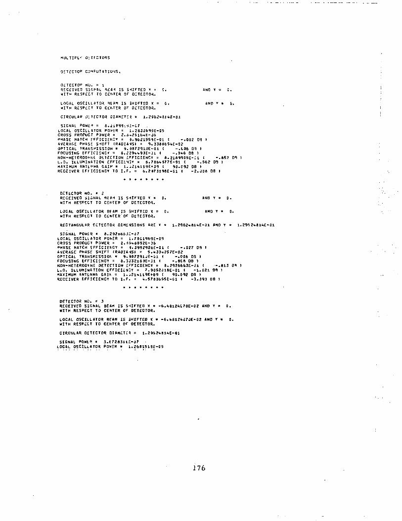
MULTIPLE O i T E C T O R S
OiTECTO0. NCI. = 1DECEIVED SIGNAL REA1 IS S-IIFTEO x = 0. AND Y = 0.WITH RESPECT TO CENTER DF 0£TESTO*.
LOCAL OSCILLATOR =)EAM IS SHIFTED X = C . AND V = 0KITH RtSPtCT TO CtKTER OF DETECTOR.
CIRCULAR Jiucioa OIAMET;« = i.z9o2*8i<.E-ojSIGNAL PQH£3 = 8.iieS9-.iI-u7
LOCAL OSCILLATOR POk>SiR = 1. 283J695E-05CROSS FROHJCT P3WER = 2. 6.,2S16»E- JD"HASE MATCH fFFICIENCY = 9. 9621559E-0 1 I - .002 09 IAVERAr .E PHASE SHIFT ( R A D I A N S ) = 9. 3388fc5l.E-a2OPTICAL TRANSMISSION = 9. 9872910E-01 t -.006 OB IFOCUSING EFFICI£NCY = 8. £291.1.9 JE- Jl ( - .Sfc6 OB )NON-HETEROO»H£ DETECTION EFFICIENCY = 8. 2189905E-C 1 ( -.852L.D. ILLUMINATION EFFICILNIY s 8. 786". 977E-01 ( -.562 09 )MAXIMUM ANUMNA GAIf' = 1. J2litll9E»09 ( 90.C92 DB IRECEIVER EFFICIENCY TO I.F. = 6. 2973198E-C1 < -2 .058 OB )
DETECTOR NO. = 2RECEI-VEO SIGNAL BEA.1 IS SHIFTED » = 0. AND Y s 0 .WITH RESPECT TO CSMTEP OF DETECTOR.
LOCAL OSCILLATOR SI AM IS SHIFTED X = C. AND Y = 0.WITH RESPECT TO CENTER OF OETESTO*.
RECTANGULAR CETECTO* DIMENSIONS ARE X c 1.296?»61UE-O1 AND Y = 1.2963u81U£-01
SIGNAL POWER = 8.292BbfcJI-fl7LOCAL OSCILLATOR POfcER = 1.78H969E-05CROSS PRODUCT POWER = 2. rt5<»S892E-36PHASE MATCH EFFICIENCY > 9.3992926e-oi ( -.02? DB iAVERAGE PHASE SHIFT (RADIA4SI = 5.<t33»257E-l)2OPTICAL TRANSMISSION = 9.98729UE-J1 ( -.006 OB )FOCUSING EFFICIENCY = 8.3J32189E-Jl I -.8C8 DB )NON-HETERODYNE DETECTION EFFICIENCY = 8.2926663E-01 ( -.813 01 IL.O. ILLUMINATION EFFICIENCY = 7.90S2018E-01 « -1.021 OB IMAXIMUM ANTLNNA GAIK = 1. i2l<«ll9E»09 ( 90.092 OB )RECEIVER EFFICIENCY TO I.F. = 4.57B3655E-01 < -3.393 OB )
DETECTOR NO. = 3RECEIVED SIGNAL BEAM IS SHIFTEO X r -6.',812'.t70E-02 AND Y sKITH RESPECT TO CENTER OF DETECTOR.
LOCAL OSCILLATOR BEAM IS SHIFTED X = -6. i.812<tiJ7 JE-03 AND Y =WITH RESPECT TO CENTER OF DETECTOR.
CIRCULAR DETECTOR OIAH£T£* - 1.2952l.81l.E-01
SIGNAL POMt" = 3.e728301£-07LOCAL OSCILLATOR POWER = 1.2681518E-05
176
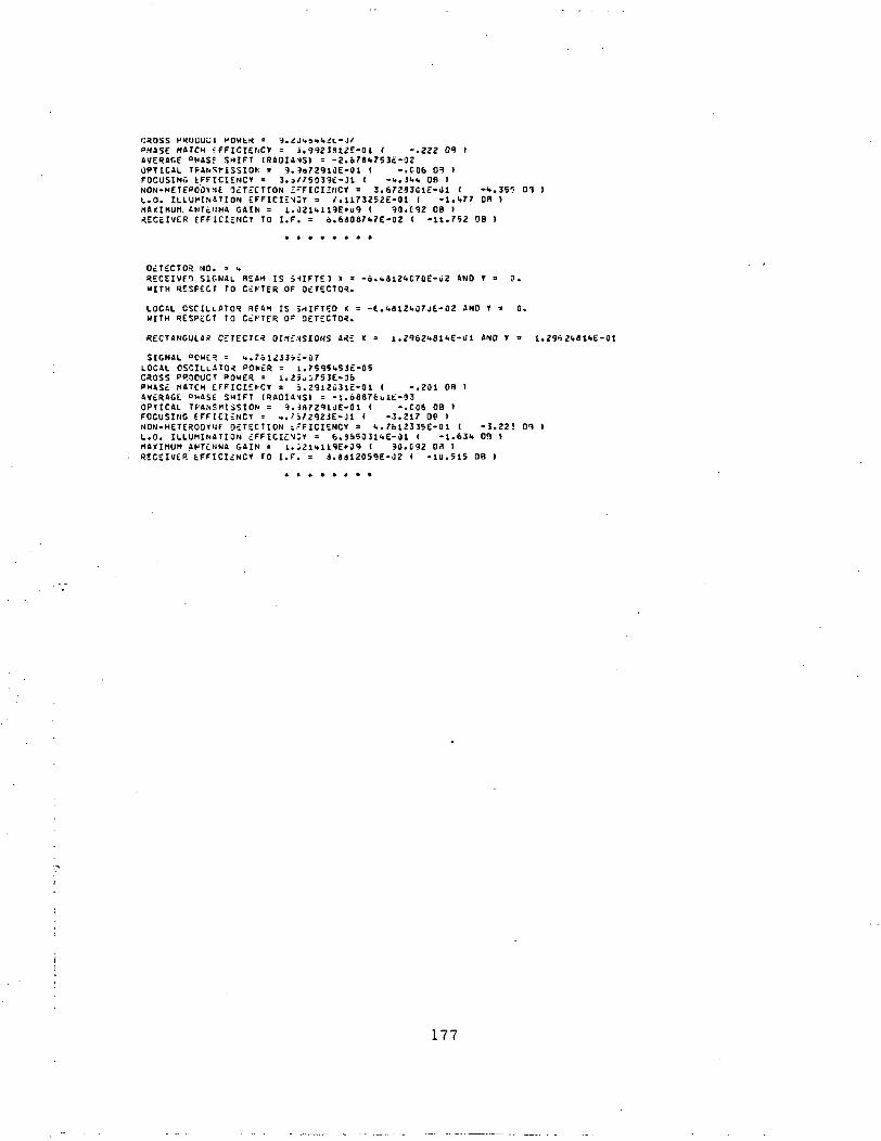
CROSS HKUUU^I HOWtK = ?. i. Ji.»»'.it-.J/'»HiSE M A T C H f F F I C I E N C V = i. 992 JSl<?£-0 I ( -.222 0"? )AVERAGE "HAS! SHIFT (RSIJIOMSI = -2.o78<«753:--02OPTICAL TPANSM3SIOK = 9.9a72910E-01 ( - .006 09 )FOCUSING EFFICIENCY = 3. b /75039E-JI ( -1..3".!. OB )NON-HETEPOO^E DETECTION £-FICIiNCr = 3.6728301E-01 < -•..SS'J 01 )L.O. ILLUMINSTION EFFICIE-<;T = /. ll7Ji5ZE-Ol ( -t.«.77 08 )nAXIHUM.ANTc.KNA GAIN = 1. Oai<.H9E»u9 ( 90.(92 08 )RECEIVER EFFICI£NCT TO I.F. = 6.6«OS7i»7E-02 ( -It.752 08 I
DETECTOR NO. = -.RECEIVFO SIGNAL BEAM IS SHIFTE1 X - -o.'.812'.C70E-u2 AND T = 0.WITH RESPECT TO C2KTER OF OtTECTO^.
LOCAL OSCILLATOR BFAM IS 3MIFTEO t = -t. 1.812U07JE-02 AND T s o.KITH RESPECT TO CctTER 0^ OETECTO*.
RECTANGULAR OETECTC* OI.tE.fSIONS A<E « = I .Z962»af.E-Ul AND V = 1.296 2I,«1<.£- 01
SIGNAL POHCR = i..roli33i£-07LOCAL OSCILLATOR POhcR = 1.7S95fc53£-05CROSS PRODUCT POMER = i.2;ui/53E-o»PHASE MATCH EFFICIErCY = i.2912031E-01 < -.201 08 IAVERAGE "MASE SHIFT (RAOIA1SI = -1.68876ult-03OPTICAL TRANSMISSION = 9.387291JE-01 ( -.C06 08 IFOCUSING EFFICIENCY = •.. 7 i?292 JE-n < -3.217 06 INON-HETERODYNf DETECTION i?FICIENCY = «.. 7612335E-01 ( -J.22! 01 )L.O. ILLUMINATION EFFICIEIIY = 6.5o50 31".E-01 ( -1.63U 03 »MAXIMUM ANTCNNA GAIN = 1. J21i»119E»59 I 30.E92 DA IRECEIVER EFFICIENCY TO I.F. = 3.8412059E-02 ( -1U.515 OB I
177