operational risk quantification mathematical solutions … · operational risk quantification...

Operational Risk QuantificationMathematical Solutions for Analyzing Loss Data

Gene Álvarez, Ph.D.May 2001

Operational Risk Quantification

Response to the 2001 Basel Committee on Banking Supervision Consultative Document on Operational Risk i

Table of Contents

Introduction ................................................................................................................................. 11 Severity Distribution for Historical Loss Data......................................................................... 1

1.1 Definition of a Tail-Adjusted Lognormal Distribution ..................................................... 11.2 Tail-Adjusted Lognormal Distribution Determination from Truncated Data................... 21.3 Which to Use: Lognormal or Tail-Adjusted Lognormal?................................................. 5

2 Capital Risk Exposure Calculation .......................................................................................... 62.1 TALN and VaR ................................................................................................................. 72.2 Which to Use: Lognormal or Tail-Adjusted Lognormal? Part II...................................... 82.3 Observed Mean versus Theoretical Mean......................................................................... 8

3 TALN versus Weibull .............................................................................................................. 94 Frequency Distribution: How to Quantify the Occurrences of Loss Events.......................... 115 Event Classification................................................................................................................ 12

5.1 When Data is Poorly Organized...................................................................................... 125.2 Loss Data Classification Scheme .................................................................................... 15

Conclusion................................................................................................................................. 16References ................................................................................................................................. 18


Response to the 2001 Basel Committee on Banking Supervision Consultative Document on Operational Risk ii

“When you can measure what you are speaking about, and express it in numbers, you know something about it; butwhen you cannot measure it, when you cannot express it in numbers, your knowledge is of a meagre andunsatisfactory kind.” William Thompson, Lord Kelvin


Response to the 2001 Basel Committee on Banking Supervision Consultative Document on Operational Risk 1

IntroductionThe daily operations of running and supporting a business are not without risk. Every organization is exposed tohuman errors, external failures, and technology breakdowns, to name just a few potential problems. Theclassification of these issues is called operational risk. The Basel Committee on Banking Supervision has definedoperational risk to be the risk of direct or indirect loss resulting from inadequate or failed internal processes,people, and systems, or from external events. Every institution is exposed to risks that fit this definition and as suchit is logical that every institution must focus on operational risk management. The ideal firm is proactive inoperational risk management: it monitors its performance by periodically assessing its personnel and departments;keeps a record of loss events that have occurred; and analyzes these losses to determine what lessons may be learnedand to develop strategies for minimizing or preventing future problems. As with all management responsibilities,there are several challenges that must be overcome before any institution will conform to this ideal. This article willaddress the issue of analyzing and quantifying loss data.

The primary objectives of quantifying operational risk are�first�to calculate the exposure of a business line,department, or firm and�second�to facilitate the process of deciding how to minimize, control, or mitigate risk.Before any calculation can be performed, though, one has to address a major obstacle: understanding thefundamental nature of the collected loss data. In other words, how can one mathematically describe the shape of agiven set of loss data? Knowing the functional form of a data set allows for great accuracy in all calculations thatderive from the data. In the coming sections, we will present a probability density function that accurately describethe monetary loss data distribution�or, a �severity distribution�, and then apply the function to calculate potentialrisk exposures. We will also discuss the choice of the frequency probability function to describe the occurrence oflosses, and the impact of this choice on operational risk quantification. And finally, a proposed operational risk lossevent classification scheme is presented in order to promote a logical structure to categorize loss events that removesmost of the uncertainty in the analysis of loss data.

1 Severity Distribution for Historical Loss Data

1.1 Definition of a Tail-Adjusted Lognormal Distribution

Generally, analysts assume that the severity distribution of operational risk monetary losses is best expressed by theLognormal function, a Normal distribution whose variable x is logarithmically transformed (x´ = Log(x)). Eventhough the body of the monetary loss distribution may be accurately described by a Lognormal curve, the tails of theempirical data are not precisely expressed by this function. Therefore, other statistical functions, such as Pareto orExtreme Value Distributions, are used to describe the tail, and the intrinsic limitation that they will not accuratelyrepresent the body is accepted. Analysts do this because catastrophic loss calculations are sensitive to the tail of thedistribution. Figure 1 illustrates the distinction between the body and tail regions of monetary loss data. Rather thanaccept the aforementioned limitation, we will describe the entire empirical data set by employing a mixture of twowell known functions: the Lognormal and Gamma functions. In mathematical literature, such mixtures are calledcompound normal distributions [1].

Body & Tail Regions of Monetary Loss Data

Tail RegionTail Region

Body Region

Figure 1: Distinction between the body and tail regions of monetary loss data when represented by a �normal� distribution.



-7.5 -5 -2.5 2.5 5 7.5

0.05

0.1

0.15

0.2

TALN & LN Distributions

LN:H0, 2, 3LTALN :H0, 2, 3.5LHm, s , kurtosisL

8.5 9 9.5 10

0.00005

0.0001

0.00015

0.0002

0.00025

0.0003

TALN & LN Distributions - Tail Comparison

LN:H0, 2, 3LTALN :H0, 2, 3.5LHm, s , kurtosisL

Figure 2: Contrast between Tail-Adjusted Lognormal and Lognormal distributions. The mean and standard deviation for each are0 and 2, while their respective kurtosis is 3.5 and 3 (definition of a normal distribution).

The motivation to use the Lognormal-Gamma mixture is simple. Because the two Lognormal parameters (mean µand standard deviation σ) reasonably depict the body of the loss distribution, a third parameter�kurtosis, or �thefourth moment��must be introduced to satisfactorily depict the tail. Parameterizing kurtosis via a Gammadistribution will result in the desired functional form. By definition, the kurtosis of a normal distribution is three;using the Lognormal-Gamma mixture, however, will allow the kurtosis parameter to be greater than or less thanthree. From this point forward, we will refer to the mixed distribution as a Tail-Adjusted Lognormal (TALN) densityfunction. A Lognormal-Gamma mixture allows an operational risk loss severity distribution to be parametricallyrepresented by a function with three parameters: mean, standard deviation, and kurtosis.

1.2 Tail-Adjusted Lognormal Distribution Determination from Truncated Data

The determination of the three parameters that depict the TALN distribution for a given set of monetary loss data iscritical. One must also keep in mind that operational risk loss data is almost always collected above a truncationthreshold because it is impractical to gather data from zero: to collect losses as small as a few cents, for example, isan impossible task. Therefore, for any given data set, the measurable quantities�µ, σ, and kurtosis�represent atruncated (conditional) distribution and not a full (unconditional) distribution. Despite this apparent limitation, all isnot hopeless. One can calculate the parameters of the full distribution from the truncated parameters. The procedureis as follows:

a) Derive the first, second, and fourth moments of the truncated TALN probability distribution function*

b) Calculate the empirical data truncated mean, standard deviation, and kurtosisc) Equate each truncated moment expression to its respective truncated measured quantity, i.e. the truncated

mean is equated to the truncated first moment equationd) Solve the three simultaneous equations.

The solution set to the three truncated simultaneous equations will yield the three unconditional parameters.

To illustrate this point, consider two TALN distributions with parameters (µ, σ, kurtosis) = (-3.50, 1.50, 3.15) and(-4.0, 1.8, 3.8). For each distribution, one hundred thousand points were randomly generated above a truncationthreshold of twenty-five thousand dollars (see Figure 3). The truncated µ, σ, and kurtosis parameters were calculatedand the simultaneous truncated moment equations were solved after each expression was set equal to its respectivemeasured truncated value. As one can readily see from Table 1 and Figure 4, the values obtained from solving theTALN simultaneous equations are in good agreement with the starting parameters. The difference is attributable tonumerical rounding in solving the equations.

Figure 4 also plots a third distribution: the Lognormal distribution if one solved the truncated Lognormal first andsecond moment equations that were equated to their respective measured quantity. Figures 4b and 4d illustrate that,even if the kurtosis turns out to be relatively small (e.g., 3.15), ignoring kurtosis will grossly misrepresent theparameterization of the tail and will, therefore, underestimate any calculation that is tail-dependent, such as VaR.

* One needs to go through the derivation only once. Retain the expressions for all future analyses.



-8 -6 -4 -2 2

0.05

0.1

0.15

0.2

0.25

3a: Generated Tail- Adjusted Lognormal Distribution

FTLN :H- 3.50, 1.50, 3.15LHm, s , kurtosisL

-8 -6 -4 -2 2

0.05

0.1

0.15

0.2

0.25

0.3

3b: Generated Tail- Adjusted Lognormal Distribution

FTLN :H- 4.0, 1.8, 3.8LHm, s , kurtosisL

Figure 3: a) Histogram of the randomly generated losses for the (µ, σ, kurtosis) = (-3.50, 1.50, 3.15) TALN density function. Losses werebinned in monetary buckets in units of $10,000. b) Histogram of the randomly generated losses for the (µ, σ, kurtosis) = (-4.0, 1.8, 3.8) TALN density function. Losses were binned inmonetary buckets in units of $10,000.

TALN Distribution Parameter Values

Given Truncated Solvedµ -3.50 -4.00 -2.43 -2.39 -3.49 -4.03σ 1.50 1.80 0.95 1.10 1.49 1.81

kurtosis 3.15 3.80 4.06 5.86 3.16 3.69

Table 1: Comparison of known conditional parameters with parameters obtained from solvingsimultaneous truncated moment equations.

Another way to determine the unconditional parameters from the truncated data set is to employ the principle ofleast squares [2]. In general, one must minimize a set of m×n simultaneous equations, where m is the number ofvariables involved in the minimization procedure and n is the number of data points used for the minimizationprocedure. Please note, the minimization of m×n equations can be numerically challenging. To demonstrate theimplementation of the principle of least squares to arrive the full parameters for a given TALN distribution, we usedthe same randomly generated data set for the (-4.0, 1.8, 3.8) TALN density as in our previous example.

We chose to minimize the TALN cumulative distribution function (cdf) and used eleven data points correspondingto 10 percentiles, ranging from 5 to 95% in units of 10%, and the constraint that the function must include the origin.Naturally, the objective function that was minimized accounted for the truncation threshold of the randomlygenerated data set. In fairness, we ran the optimization program three times: once without weight and twice with

different weights. The weights used, to remove subjectivity, were 1)1( −− iy and 1

1

−

=��

��

��

k

iii nn , where (xi, yi) is the

ith cdf point for a given momentary amount and its corresponding percentile, and ni is the number of losses for the ith

point. The results from the three fits are listed in Table 2 and the parameters of the two weighted results areillustrated in Figure 5. Even with a casual glance at either Table 2 or Figure 5, one can surmise that the three 3-parameter sets obtained via the principle of least squares are not in good agreement with the original parameters.One may argue that 11 points are not a sufficient number of points to use in an optimization method; however, onemust keep in mind that the number of equations to be optimized is 3n�. Hence, the computational complexityincreases geometrically. In contrast, our first discussed method required solving three simultaneous equations todetermine the three parameters of the full TALN function to represent the empirical data�far more simple,efficient, and elegant.

� For every data point, one must optimize three equations for each unknown parameter: µ, σ, and kurtosis.



4.5 5 5.5 6

0.00005

0.0001

0.00015

4d: Overlay of 2 TALN & 1 LN Distributions - Tail Comparison

LN:H- 6.07, 2.45, 3.00LTALN :H- 4.03, 1.81, 3.69LTALN :H- 4.00, 1.80, 3.80LHm, s , kurtosisL-15 -12.5 -10 -7.5 -5 -2.5 2.5

0.05

0.1

0.15

0.2

0.25

4c: Overlay of 2 TALN & 1 LN Distributions

LN:H- 6.07, 2.45, 3.00LTALN :H- 4.03, 1.81, 3.69LTALN :H- 4.00, 1.80, 3.80LHm, s , kurtosisL4.5 5 5.5 6

1´ 10-6

2´ 10-6

3´ 10-6

4´ 10-6

5´ 10-6

6´ 10-6

4b: Overlay of 2 TALN & 1 LN Distributions - Tail Comparison

LN:H- 3.64, 1.55, 3.00LTALN :H- 3.49, 1.49, 3.16LTALN :H- 3.50, 1.50, 3.15LHm, s , kurtosisL-10 -8 -6 -4 -2 2 4

0.05

0.1

0.15

0.2

0.25

4a: Overlay of 2 TALN & 1 LN Distributions

LN:H- 3.64, 1.55, 3.00LTALN :H- 3.49, 1.49, 3.16LTALN :H- 3.50, 1.50, 3.15LHm, s , kurtosisL

Figure 4: Comparison between TALN and LN distributions whose parameters were obtained from solving simultaneoustruncated moment equations, and the original TALN distribution (solid curve).



TALN Distribution Parameter Values

-10 -8 -6 -4 -2 2 4

0.2

0.4

0.6

0.8

5a: Overlay of 3 TALN Distributions

H- 2.09,1.45,3.33LH- 2.43,0.42,3.00LH- 4.00, 1.80, 3.80LHm, s , kurtosisL

4.5 5 5.5 6

0.00005

0.0001

0.00015

5b: Overlay of 3 TALN Distributions - Tail Comparison

H- 2.09,1.45,3.33LH- 2.43,0.42,3.00LH- 4.00, 1.80, 3.80LHm, s , kurtosisL

Figure 5: Comparison between the two TALN distributions whose parameters were obtained via the Principle of Least Squares and theoriginal TALN distribution (solid curve).

One may also use the Adaptive Grid Refinement (AGR) algorithm [3] to determine the unconditional parameters.AGR is an n-dimensional adaptation of Newton�s method related to adaptive mesh generation. Even though AGRwill find all possible solutions over the defined region of possible solutions, the limitations of the algorithm are: i) itdoes not allow constraints; and ii) it does not define the optimal solution region. The second limitation requires auser to define a sufficiently large grid region to capture all possible solutions, if such a region can be defined. Forexample, the solution space for the µ must be large enough to anticipate any potential solution. Otherwise, theresults found in the smaller solution space for the mean may not be the true optimal answers. One will have similarconcerns for the other two parameters: σ and kurtosis. Hence, one must define a three dimensional grid, withgranular lattice spacing, sufficiently large enough to accommodate any possible solution combination for the threeparameters. Clearly, it is more desirable to solve the TALN truncated moment equations to obtain the exact solutionsfor the full distribution parameters than to deal with the limitations and complications of the AGR algorithm.

1.3 Which to Use: Lognormal or Tail-Adjusted Lognormal?

Given a truncated data set, one is able to calculate the truncated mean, standard deviation, and kurtosis parameters.Then what? How does one choose between the Lognormal and TALN density functions to obtain the fulldistribution that represents the data? If the truncated kurtosis is extremely large�e.g. greater than six�then oneshould choose the TALN density. But in other cases, the measured truncated kurtosis will not be such an obviousindicator. The solution to this dilemma is straightforward: solve the truncated moment equations for both the LN andTALN distributions, then perform an Anderson-Darling goodness-of-fit test to resolve the indecisiveness.

Let us consider an example to demonstrate this point. We begin with a known LN distribution with µ = -3.5 and σ =1.5 and generate two-hundred-fifty thousand random losses above the truncation point of $25,000 (see Figure 6a).The truncated parameters calculated for the generated data set are (µ, σ, kurtosis) = (-2.42, 0.94, 3.71). For the LNand TALN densities, we solve their respective simultaneous set of truncated moment equations. The solution for the

Given Fitted Parameter Values

No Weight Weight: 1)1( −− iy Weight: 1

1

−

��

��=

k

i inin

µ -4.00 -2.45 -2.43 -2.09σ 1.80 0.72 0.42 1.45

kurtosis 3.80 3.03 3.00 3.33

Table 2: Comparison of known conditional parameters with parameters obtained via the Principle of LeastSquares.



full TALN distribution is (µ, σ, kurtosis) = (-3.37, 1.46, 3.04), while for the full LN distribution we obtain (µ, σ) =(-3.51, 1.51). Figures 6b and 6c depict the resultant curves.

-8 -6 -4 -2 2

0.05

0.1

0.15

0.2

0.25

6a: Generated Lognormal Distribution

LN:H- 3.50 , 1.50, 3.0LHm, s , kurtosisL

-8 -6 -4 -2 2

0.05

0.1

0.15

0.2

0.25

6b: FTLN & LN Distributions

LN:H- 3.51, 1.51, 3LFTLN :H- 3.37, 1.46, 3.04LHm, s , kurtosisL

2.5 3.5 4 4.5

0.00002

0.00004

0.00006

0.00008

0.0001

6c: FTLN & LN Distributions - Tail Comparison

LN:H- 3.51, 1.51, 3LFTLN :H- 3.37, 1.46, 3.04LHm, s , kurtosisL

Figure 6: a) Histogram of the randomly generated losses for the (µ, σ) = (-3.50, 1.50) LN density function. Losses were grouped in monetarybuckets in units of $10,000.b,c) Comparison between TALN and LN distributions that describe the generated data as shown in Fig. 6a.

To choose between the two densities, one may apply either the Chi-Square or Kolmogorov-Smirnov goodness-of-fittest. However, the Anderson-Darling test should be employed instead, because it gives more weight to the tail of thedistribution. This is an important criterion since the slope of the tail reflects the sensitivity of the distribution. Whenwe calculated the AD-test value for each of the resultant distributions, the TALN value was approximately twopercent smaller than the LN value. In this example, given that we started out with a known LN distribution, theTALN turned out to be the better fit. The minute discrepancy in the quality of fit is due to numerical round-off errorsin solving the respective sets of truncated equations. Thus, in general, the TALN density function will adequatelydescribe the severity distribution of the monetary loss data, even when a LN distribution may be used. When wediscuss VaR calculations in section 2.2, we will return to this example.

2 Capital Risk Exposure CalculationIn the analysis of data, a closed, analytical function is advantageous because it produces a continuous depiction ofthe underlying data set. The analytical function can be evaluated to obtain values of the function or of its inverse (ifone exists), for various numerical calculations. In this section, we will demonstrate the application of the TALNprobability density function in capital risk exposure calculations, and discuss its advantages.

Before we proceed, we must note that, although empirical data can be grouped in discrete monetary buckets tocalculate values such as probabilities, this practice must be used with caution. If we limit our discussion toprobability calculations�unless the data is smooth throughout the entire data capture range, and is of statisticalsignificance to estimate probabilities with small errors�we will underestimate or overestimate the probabilities andproduce inaccurate values. And, if one needs a probability value beyond the captured monetary range, interpolation



of the data definitely will result in erroneous numbers. One of the virtues of a parameterized functional form is thatthese shortcomings can be avoided.

2.1 TALN and VaR

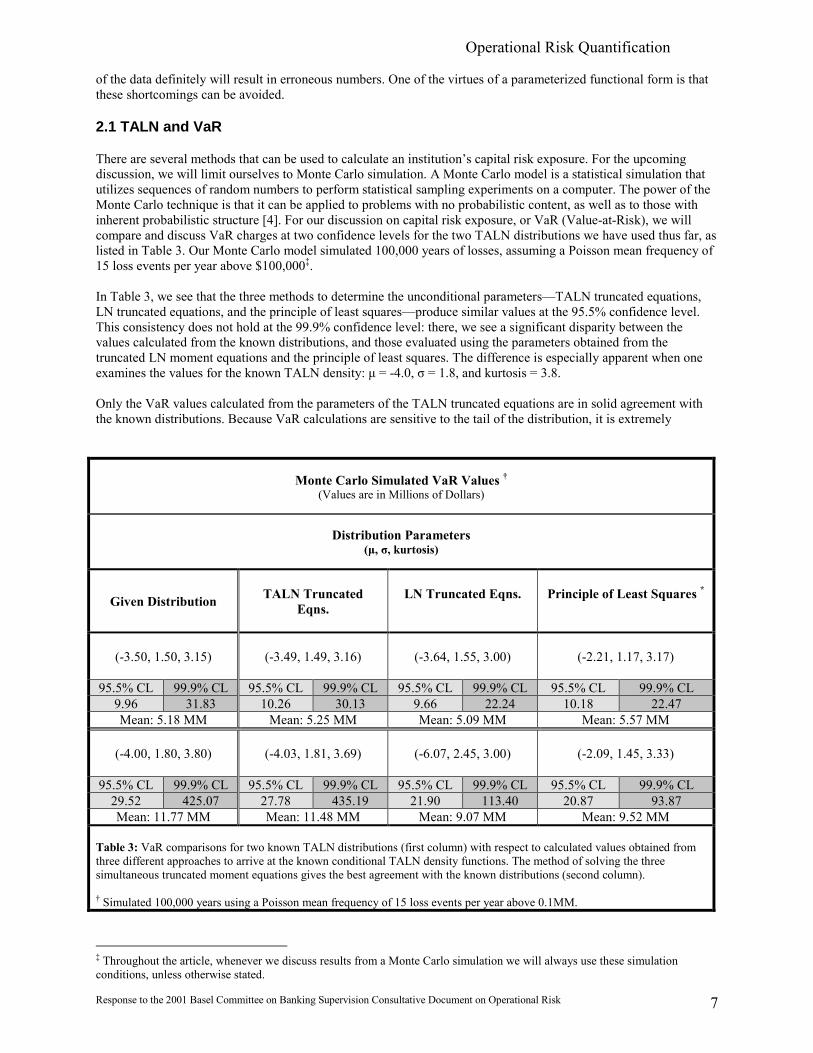
There are several methods that can be used to calculate an institution�s capital risk exposure. For the upcomingdiscussion, we will limit ourselves to Monte Carlo simulation. A Monte Carlo model is a statistical simulation thatutilizes sequences of random numbers to perform statistical sampling experiments on a computer. The power of theMonte Carlo technique is that it can be applied to problems with no probabilistic content, as well as to those withinherent probabilistic structure [4]. For our discussion on capital risk exposure, or VaR (Value-at-Risk), we willcompare and discuss VaR charges at two confidence levels for the two TALN distributions we have used thus far, aslisted in Table 3. Our Monte Carlo model simulated 100,000 years of losses, assuming a Poisson mean frequency of15 loss events per year above $100,000�.

In Table 3, we see that the three methods to determine the unconditional parameters�TALN truncated equations,LN truncated equations, and the principle of least squares�produce similar values at the 95.5% confidence level.This consistency does not hold at the 99.9% confidence level: there, we see a significant disparity between thevalues calculated from the known distributions, and those evaluated using the parameters obtained from thetruncated LN moment equations and the principle of least squares. The difference is especially apparent when oneexamines the values for the known TALN density: µ = -4.0, σ = 1.8, and kurtosis = 3.8.

Only the VaR values calculated from the parameters of the TALN truncated equations are in solid agreement withthe known distributions. Because VaR calculations are sensitive to the tail of the distribution, it is extremely

Monte Carlo Simulated VaR Values �(Values are in Millions of Dollars)

Distribution Parameters(µ, σ, kurtosis)

Given Distribution TALN TruncatedEqns.

LN Truncated Eqns. Principle of Least Squares *

(-3.50, 1.50, 3.15) (-3.49, 1.49, 3.16) (-3.64, 1.55, 3.00) (-2.21, 1.17, 3.17)

95.5% CL 99.9% CL 95.5% CL 99.9% CL 95.5% CL 99.9% CL 95.5% CL 99.9% CL9.96 31.83 10.26 30.13 9.66 22.24 10.18 22.47Mean: 5.18 MM Mean: 5.25 MM Mean: 5.09 MM Mean: 5.57 MM

(-4.00, 1.80, 3.80) (-4.03, 1.81, 3.69) (-6.07, 2.45, 3.00) (-2.09, 1.45, 3.33)

95.5% CL 99.9% CL 95.5% CL 99.9% CL 95.5% CL 99.9% CL 95.5% CL 99.9% CL29.52 425.07 27.78 435.19 21.90 113.40 20.87 93.87Mean: 11.77 MM Mean: 11.48 MM Mean: 9.07 MM Mean: 9.52 MM

Table 3: VaR comparisons for two known TALN distributions (first column) with respect to calculated values obtained fromthree different approaches to arrive at the known conditional TALN density functions. The method of solving the threesimultaneous truncated moment equations gives the best agreement with the known distributions (second column).

� Simulated 100,000 years using a Poisson mean frequency of 15 loss events per year above 0.1MM.

� Throughout the article, whenever we discuss results from a Monte Carlo simulation we will always use these simulationconditions, unless otherwise stated.



* Corresponding to the parameters obtained using 1

1

−

��

��=

k

i inin as weights.

important to correctly parameterize the tail to avoid under- or over-estimated VaR values. In practice, with anaccurate functional representation of the data set in question, capital risk exposure calculations can be carried out tothree standard deviations (~ 99.73% confidence level§) with mathematical certainty.

2.2 Which to Use: Lognormal or Tail-Adjusted Lognormal? Part II

In section 1.3 we discussed, given a truncated data set, which of the two density distributions�TALN or LN�should be used. We demonstrated, at least via the Anderson-Darling test, that the two functional forms wereadequate mathematical representations for the example we used. For thoroughness, we will compare the VaR valuesfor the known distribution, to the values for the solved TALN and LN parameters. The results of this comparison aregiven in Table 4. As in our previous VaR calculation exercise, we simulated 100,000 years of losses, assuming aPoisson mean frequency of 15 loss events per year above $100,000. As one can see from Table 4, the choice ofprobability density function does not significantly affect the VaR results in comparison with the VaR values of theknown LN density function, so the choice of a TALN density did not skew any VaR calculation.

VaR Comparisons(Values are in Millions of Dollars)

Distribution Parameters Mean 95.5% CL 99.9% CLµ = -3.50, σ = 1.50 4.971 9.293 21.508µ = -3.51, σ = 1.51 4.982 9.212 20.694µ = -3.37, σ = 1.46, kurtosis = 3.04 4.974 9.372 20.346

Table 4: Comparison of VaR values of a known LN distribution (first row) againstthose calculated from solving the LN and TALN truncated moment equations. Twohundred fifty thousand losses above $25,000 were randomly generated for the knowndistribution. The truncated parameters were (µ = -2.42, σ = 0.94, kurtosis = 3.71).The VaR values are a result of a simulation of 100,000 years, with a Poissonmean frequency of 15 loss events per year above 0.1MM.

2.3 Observed Mean versus Theoretical Mean

Let us now focus our attention on the importance of distinguishing between the theoretical mean and the observedmean. The theoretical mean is simply the mean value of a density distribution (the first moment), while the observedmean is the mean of a truncated data set. As we have noted, operational risk loss data is invariably truncated. Hence,the observed mean does not equal the theoretical mean: it may be below or above the theoretical mean depending onthe truncation threshold. As a result, any calculation that relies on the observed mean, as proxy for the theoreticalmean, will give misleading results.

One VaR proposal under consideration would apply a multiplicative factor to the three-year average of the meanaggregate loss. Assuming an institution has a good procedure to capture data on loss events and their monetaryimpact, the truncated mean aggregate loss for a given year may be calculated fairly accurately. One the other hand,results will not be accurate for the mean of the underlying full severity distribution, which describes the collectedloss data. To quantify this assertion, we simulated 1000 years for two known TALN distributions to calculate thetwo and three year average of the mean aggregate loss (observed mean) for two different Poisson mean frequenciesabove the $25,000 threshold. The frequency of 13 events per year could represent a very good control environment,while 40 events per year could represent an average control environment. Table 5 summarizes the results. All thecalculations produced outcomes in which 90% of the observed means were above the theoretical mean and, in somecases, this percentage was as high as 100%. Hence, anyone using the observed mean as a substitute for the

§ For simplicity, the author prefers the 99.9% confidence level.



theoretical mean in any monetary calculation must keep in mind that this replacement may grossly overestimate theactual amount.

Observed Mean vs. Theoretical Mean

Observed Mean Percentage Below / Above Theoretical Mean

TALN Distribution Parameters

µ = -3.50, σ = 1.50, kurtosis = 3.15 µ = -4.00, σ = 1.80, kurtosis = 3.80

Poisson Frequency 2 Year Average 3 Year Average 2 Year Average 3 Year Average

13

40

8.2% / 91.8%

0.2% / 99.8%

2.1% / 97.9%

0% / 100%

6.0% / 94.0%

0% / 100%

2.4% / 97.6%

0% / 100%

Table 5: Monte Carlo simulation results that calculate the percentage of time the observed mean is below orabove the theoretical mean for two distinct TALN distributions. For each Monte Carlo run, 1000 years weresimulated using Poisson mean frequencies of 13 and 40 to generate the n random loss events per year above$25K.

Furthermore, using only the mean does not take into account all that is needed to accurately describe the severitydistribution�particularly the risk profile of an institution. One cannot neglect the volatility, as measured by thestandard deviation, and the �heaviness� of the tail, as measured by kurtosis, because�as we have seen in variousnumerical examples�using the three parameters together enables a risk analyst to perform calculations withconfidence and mathematical certainty.

3 TALN versus WeibullBecause of its simple functional form and ease of use, the Weibull distribution is occasionally used to describemonetary loss data. But how reliable is the Weibull distribution in depicting loss data? It is important that thefunction we choose to describe the monetary distribution of loss events gives an accurate representation of theunderlying data set. Otherwise, all results will be questionable. In this section, we will discuss the Weibull density�saccuracy in representing monetary loss data and the calculated VaR values. In all of our work we will employ aWeibull distribution with three parameters: location (ξ), scale (c), and shape (α).

As we have done thus far, let us consider an example. We will begin with a TALN distribution with parameters (µ,σ, kurtosis) = (-4.0, 1.8, 3.8), and a Weibull distribution with parameters (ξ, c, α) = (-12.0, 4.5, 8.8). For the twogiven densities, we will randomly generate 100,000 losses without any truncation threshold (see Figures 7a and 7b).As illustrated in Figure 7c, we will combine these two data sets to create one with 200,000 losses. Now, we willobtain the TALN and Weibull parameters that best represent the merged data set. To arrive at the respective set of

parameters, we will use the principle of least squares using 1

1

−

=��

��

��

k

iii nn as weights**. Figures 7d and 7e illustrate

the results of the fits. As one can see, the Weibull distribution does not represent the data set as well as the TALNdistribution. To quantify what the eye �knows�, the Anderson-Darling goodness-of-fit test value for the TALN isapproximately 60% lower than the Weibull value. Therefore, one can confidently conclude that the TALNdistribution better describes the mixed losses.

** We used 100 points in the fit, corresponding to the hundred buckets used to group the data as shown in Figure 7.



-12.5 -10 -7.5 -5 -2.5 0 2.5 5

0.05

0.1

0.15

0.2

0.25

7a: Generated TALN Distribution

-10 -8 -6 -4 -2 0 2

0.05

0.1

0.15

0.2

7b: Generated Weibull Distribution

-12.5 -10 -7.5 -5 -2.5 0 2.5 5

0.05

0.1

0.15

0.2

7c: TALN + Weibull Generated Distributions

-12.5 -10 -7.5 -5 -2.5 0 2.5 5

0.05

0.1

0.15

0.2

7d: Weibull Fit

-12.5 -10 -7.5 -5 -2.5 0 2.5 5

0.05

0.1

0.15

0.2

7e: TALN Fit

Figure 7: a) Histogram of the randomly generated losses for the (µ, σ, kurtosis) = (-4.0, 1.8, 3.8) TALN density function, asshown by the solid curve.b) Histogram of the randomly generated losses for the (ξ, c, α) = (-12.0, 4.5, 8.8) Weibull density function, as shown by the solidcurve.c) Addition of histogram 7a plus 7b.d) Histogram created when fitted Weibull distribution is overlaid on Fig. 7c. The Weibull distribution shown in Fig. 7d was

obtained via the principle of least squares using1

1

−

��

��=

k

i inin as weights.

e) Histogram created when fitted TALN distribution is overlaid on Fig. 7c. The TALN distribution shown in Fig. 7e was obtained

via the principle of least squares using1

1

−

��

��=

k

i inin as weights.

Continuing with our example, we will calculate the VaR values�� for the original distributions and the two fitteddistributions. At the 99.9% confidence level, one might expect the VaR quantity for the combined data set to be thesame order of magnitude as the average of the individual 99.9% confidence level values for the original data sets.One may propose this �guesstimate� since the losses in the tail of the original TALN distribution will influence thecalculation, even though the width of the combined data set is wider than the two original distributions. As shown inTable 6, the fitted Weibull distribution grossly underestimates the VaR result, while the fitted TALN distributionagrees with our educated guess.

Qualitatively, a risk manager can conclude from this example that if a business has experienced large monetarylosses, the Weibull distribution will not accurately depict the severity distribution, and that VaR calculations based

�� Monte Carlo simulations of 100,000 years of losses assuming a Poisson mean frequency of 15 loss events per year above$100,000.



on the Weibull density will result in imprecise values. As demonstrated, the TALN distribution will describe the tailof the monetary loss distribution with better accuracy and higher precision.

VaR Comparisons(Values are in Millions of Dollars)

VaR Values for each RandomlyGenerated 10,000 Losses

VaR Values for the Combined 20,000Losses for each Fitted Distribution

TALN(µ, σ, kurtosis) =(-4.0, 1.8, 3.8)

Weibull(ξ, c, α) =

(-12.0, 4.5, 8.8)

TALN(µ, σ, kurtosis) =

(-3.97, 2.06, 3.17)

Weibull(ξ, c, α) =

(-11.12, 4.74, 8.15)VaRs: Mean 11.77 6.40 11.93 5.33

95.5% CL 29.52 12.39 29.94 9.6399.9% CL 425.07 27.13 237.43 17.32

Table 6: VaR comparison between the original data sets as generated for the given distribution (first twocolumns) and the combined data set as fitted by the TALN and Weibull distributions (last two columns).The VaR values are a result of a simulation of 100,000 years, with a Poisson mean frequency of 15 lossevents per year above 0.1MM.

4 Frequency Distribution: How to Quantify the Occurrences of Loss EventsIdentifying the severity (monetary) distribution of loss event data with the best descriptive mathematical functionalform is vital. But the analysis is not complete until one also has determined how to quantify the occurrence of lossevents. The latter is equally important because the frequency distribution directly reflects the number of loss eventsone might expect to experience over a certain time horizon. For our investigation, we will consider three relateddiscrete distributions to portray the frequency of loss events.

The three discrete distributions we will use are the binomial, negative binomial, and the Poisson distributions. Allthree satisfy the same recursive relationship and are described by one parameter or two [5]. The distinction amongthe three distributions is the relationship between the mean and the variance. For the binomial distribution, thevariance is less than the mean; for the negative binomial distribution, the variance is greater then the mean; and, forthe Poisson distribution, the variance and the mean are equal.

To illustrate the effect of the choice of frequency distribution, we calculate the VaR values implementing Panjer�srecursive algorithm [6] for the two TALN distributions: (µ, σ, kurtosis) = (-3.50, 1.50, 3.15) and (-4.0, 1.8, 3.8).Panjer�s algorithm was used to avoid any dependency on the random sampling of the monetary interval as it is donein Monte Carlo simulations. For the (-3.50, 1.50, 3.15) density, we assumed the mean frequency for all threefrequency distributions was 72 loss events, while the variances were 10, 25, 50, and 75% of the mean value for thebinomial and negative binomial distributions. For the other severity distribution in our example, we assumed themean frequency for all three frequency distributions was 95 loss events and changed the variance as previouslystated. The mean frequency represents the total number of loss events an institution may experience: the monetarythreshold is zero dollars��. A summary of the results is listed in Table 7.

As Table 7 illustrates, the choice of frequency distribution does not greatly influence the calculated VaR values,even though, as expected, the values do increase�but only slightly, as the variance increases. Therefore, any of thethree discrete distributions mentioned could be used to describe the occurrence of loss events without great concernon the impact on VaR calculations.

One important observation is that, for the known TALN distribution, the VaR values calculated using Panjer�srecursive algorithm and the Monte Carlo simulation given in Table 3 are consistent with each other. As long asfrequencies are related via conditional probabilities, the results of VaR calculations will be similar, whether one iscalculating from zero dollars or from another monetary truncation point.

�� The mean frequencies of 72 and 95 loss events per year from the threshold of zero dollars are consisted for each known TALNdistribution if one assumes 15 loss events above 0.1MM for both densities, as we did in our Monte Carlo simulations.



VaR Comparisons for Three Frequency DistributionsVaR Values are in Millions of Dollars

(µ, σ, kurtosis) =(-3.50, 1.50, 3.15) Binomial

Mean = 72Poisson

Mean = 72Negative Binomial

Mean = 72Variance 7.2 18.0 36.0 54.0 72.0 79.2 90.0 108.0 126.0

VaRs: Mean 6.51 6.51 6.52 6.52 6.52 6.52 6.52 6.52 6.5295.5% CL 11.96 12.00 12.06 12.12 12.18 12.20 12.24 12.30 12.3699.9% CL 34.15 34.17 34.21 34.25 34.28 34.30 34.32 34.36 34.40

(µ, σ, kurtosis) =(-4.00, 1.80, 3.80) Binomial

Mean = 95Poisson

Mean = 95Negative Binomial

Mean = 95Variance 9.5 23.75 47.50 71.25 95.00 104.50 118.75 142.50 166.25

VaRs: Mean 14.17 14.18 14.19 14.19 14.19 14.19 14.19 14.19 14.1995.5% CL 34.27 34.38 34.56 34.73 34.90 34.96 35.07 35.24 35.4299.9% CL 453.72 454.00 454.52 455.05 455.45 455.72 455.98 456.51 457.04

Table 7: Two scenarios demonstrate the influence of frequency distributions on the VaR calculations. The VaRvalues increase, but only slightly, as the variance increases. The monetary step size of 0.005MM was used forall Panjer�s recursive algorithm calculations.

5 Event Classification

5.1 When Data is Poorly Organized

We have now seen the significance of properly characterizing the severity distribution of monetary loss data. With aprecise mathematical depiction of the data one is analyzing, calculations become meaningful and precise. However,regardless of the tools at one�s fingertips and the mathematical rigor of the tools, if the data under analysis issuspect, then the results are meaningless. That is why good classification of data is vital. It must be doneconsistently, and it must follow a logical pattern. If the data is categorized haphazardly, any values derived from thedata will reflect its irregularity. When we talk about categorizing data, we mean that we are grouping loss eventsbased on their causes. Some classifications schemes advocate grouping events by their effects, but this system doesnot give us useful information about where losses come from. Such categorization methods lead to logicalinconsistencies and yield erroneous calculated values.

Before we proceed, let us understand the distinction between cause and effect categories. The cause of an event isthe action or set of circumstances that led to the event. Effect is the monetary or non-monetary loss that is incurreddue to the event. In our discussion, we will not consider non-monetary losses because they are inherently difficult toquantify.

Let us now consider the following example on the importance of not misclassifying loss events. We will simplyassume that we have two cause categories, fraud and sales misrepresentation, and two effect categories, regulatoryfines and lawsuit settlements. If one followed an effect classification scheme, then one could have both fraud andsales misrepresentation loss events in the same class even though the two categories, from a managementperspective, are quite distinct.

To quantify the above point, let us take into account four examples. Once again, we will employ our two favoriteTALN distributions: (µ, σ, kurtosis) = (-3.50, 1.50, 3.15) and (-4.0, 1.8, 3.8). Assume the first distribution representsfraud related losses, while the second represents losses caused by sales misrepresentation. Given the one hundredthousand randomly generated losses for each distribution, we examine four scenarios. The first two scenariosexamine misclassification of losses above a $50,000 threshold. The second pair examines losses with amountsgreater than $100,000. For each pair of scenarios, the first example will show the results when salesmisrepresentation losses are mixed into the set of fraud events. In the second example, fraud losses will be mixed



into the sales misrepresentation losses. Because the four cases are analogous, we will outline the applied procedurefor one and state the results for all, as shown in Table 8.

Results from Mixing Losses Between Two Known TALN Distribution

TALN Distribution Parameters(µ, σ, kurtosis)

Given Truncated: Before Mixture Truncated: After Mixture Solved

Scenario 1: A random selection of losses greater than 0.05MM from (-4.00, 1.80, 3.80) are mixed into (-3.50, 1.50, 3.15) VaR Values are in Millions of Dollars

A (-4.00, 1.80, 3.80) (-2.39, 1.10, 5.86) (-2.53, 1.08, 6.38) (-5.01, 2.03, 3.91)B (-3.50, 1.50, 3.15) (-2.43, 0.95, 4.06) (-2.32, 0.98, 4.78) (-2.93, 1.33, 3.96)

A B A BVaRs: Mean 12.27 5.25 23.39 7.11

95.5% CL 30.44 10.26 45.67 15.0999.9% CL 461.38 30.74 1266.71 100.82


C (-3.50, 1.50, 3.15) (-2.43, 0.95, 4.06) (-2.56, 0.94, 4.35) (-5.05, 1.94, 2.41)D (-4.00, 1.80, 3.80) (-2.39, 1.10, 5.86) (-2.31, 1.07, 5.56) (-3.11, 1.50, 4.27)

C D C DVaRs: Mean 5.25 12.27 9.74 11.58

95.5% CL 10.26 30.44 23.50 26.1099.9% CL 30.74 461.38 334.93 378.12


E (-4.00, 1.80, 3.80) (-2.39, 1.10, 5.86) (-2.55, 1.02, 7.19) (-4.65, 1.85, 4.31)F (-3.50, 1.50, 3.15) (-2.43, 0.95, 4.06) (-2.30, 1.02, 4.39) (-3.08, 1.45, 3.56)

E F E FVaRs: Mean 12.27 5.25 24.04 7.55

95.5% CL 30.44 10.26 44.02 15.9499.9% CL 461.38 30.74 1121.34 84.48


G (-3.50, 1.50, 3.15) (-2.43, 0.95, 4.06) (-2.57, 0.89, 4.88) (-4.03, 1.54, 3.10)H (-4.00, 1.80, 3.80) (-2.39, 1.10, 5.86) (-2.28, 1.11, 5.12) (-3.38, 1.66, 3.76)

G H G HVaRs: Mean 5.25 12.27 4.04 12.27

95.5% CL 10.26 30.44 7.80 27.6199.9% CL 30.74 461.38 27.95 273.43

Table 8: Four scenarios demonstrate the effect on VaR values when one randomly mixes the losses between two known TALN severitydistributions. The VaR values are a result of a simulation of 100,000 years, with Poisson mean frequencies of 13 and 17 monetary loss eventsper year above 0.1MM.



Let us begin with the first scenario, which is sales misrepresentation events categorized with fraud. In our example,loss events above $50,000 that belong in the (µ, σ, kurtosis) = (-4.0, 1.80, 3.80) TALN distribution are one-third ofthe time collected with events from the (µ, σ, kurtosis) = (-3.50, 1.50, 3.15) TALN distribution and the total numberof losses remains the same (for us, that is 200,000). As a result, the two distributions are now altered�theirparameters differ from what they should actually be. In scenario one, the (-4.0, 1.80, 3.80) distribution, because itlost events above 0.05MM, has been transformed into a severity density with parameters (-5.01, 2.03, 3.91). The(-3.50, 1.50, 3.15) density, because it has gained events above 0.05MM, has been transformed into a TALN densitywith (-2.93, 1.33, 3.96).

The impact of the transformations�the misclassification of loss events�is profound. As Table 8 illustrates, thecalculated VaRs at the 99.9% confidence level for the two �new� TALN density functions are starkly different fromthe known TALN distributions. The VaR results increased approximately three times from the original calculatedresults. If one believes this problem can be resolved by taking an appropriate combination of the altered VaRnumbers via a correlation analysis to arrive back at the original VaR values, such reasoning is flawed. Thisconclusion assumes a priori knowledge of the original VaR results, which we all know is not possible: if monetarylosses and their occurrence could be predicted with certainty, there would be no need for a risk managementdepartment.

To exemplify the power and usefulness of the TALN density, we should note that, in scenario two, the altereddistribution for the (-3.50, 1.50, 3.15) TALN density is (-5.05, 1.94, 2.41)�a density function with kurtosis lessthan three. As previously noted, the Lognormal-Gamma mixture allows one to have kurtosis values less than three.

A similar metamorphosis of the severity distribution will occur if one does not properly identify a loss event and itscorresponding monetary impact. Let us consider, for example, a case in which a few loss events above $100,000 arenot identified as one event, but as several different events, even though they are all classified in the same category.Using the (µ, σ, kurtosis) = (-4.0, 1.80, 3.80) TALN distribution, we randomly chose events with monetary amountsgreater than $100,000 and divided these amounts into two or three components. The new truncated parameters are(-2.01, 1.28, 2.42). For the new truncated parameters there was no solution to the truncated TALN momentequations. Consequently, one had to solve the truncated lognormal moment equations. When one solved thesimultaneous equations, the parameters for the new data set are (µ, σ) = (-3.83, 2.17). This time, the TALNdistribution is transformed into a LN distribution, and the VaR at the 99.9% confidence level was greatlyunderestimated, as shown in Table 9. The Monte Carlo simulation did take into account the new frequency of lossevents above $100,000 that resulted from splitting the losses.

Results from Splitting Losses from a Known TALN Distribution

TALN Distribution Parameters(µ, σ, kurtosis)

Given Truncated:Before Split of Losses

Truncated:After Split of Losses

Solved

(-4.00, 1.80, 3.80) (-2.39, 1.10, 5.86) (-2.01, 1.28, 2.42) (-3.83, 2.17, 3.00)VaRs: Mean 12.27 10.55

95.5% CL 30.44 28.3099.9% CL 461.38 166.02

Number of Events 100,000 118,562

Table 9: A scenario that demonstrates the effect on VaR values when one randomly splits losses from a known TALN severitydistribution. The VaR values are a result of a simulation of 100,000 years, with a Poisson mean frequency of 15 loss events peryear above 0.1MM for the TALN density and a Poisson mean frequency of 12 loss events per year above 0.1MM for the LNdensity.



The two arguments just presented illustrate that, when operational risk managers collect data, they must use a logicaland consistent classification scheme, with mutually exclusive categories, and coherent definitions for losses andtheir corresponding monetary impacts. Quantitative analysis is only as good as the data upon which it is based, andif operational risk calculations are done using an unsound classification scheme, any results will be suspect.

-10 -8 -6 -4 -2 2 4

0.05

0.1

0.15

0.2

0.25

LN:H- 3.83, 2.17, 3.00LFTLN :H- 4.00, 1.80, 3.80LHm, s , kurtosisL

4.5 5 5.5 6

0.00005

0.0001

0.00015

0.0002

0.00025

Tail Comparison

LN:H- 3.83, 2.17, 3.00LFTLN :H- 4.00, 1.80, 3.80LHm, s , kurtosisL

Figure 9: Histograms depict the change to a TALN distribution (solid curve) when losses are spilt (dash curve).

5.2 Loss Data Classification Scheme

It is essential to clearly define an �operational risk loss event� and its corresponding �monetary impact,� and tocategorize loss events in statistically non-overlapping classification groups. As with any analysis, one should alwaysbe mindful of the acronym GIGO�garbage in, garbage out. To keep from producing �garbage,� we propose thatoperational risk loss events be grouped into the following five major categories.

1) Employee: loss events resulting from the actions, or inactions, of a person who works for another in returnfor stipulated services.

2) Business Process: loss events arising from a firm�s execution of business operations.

3) Relationships: loss events caused by the connection or contact that a firm has with clients, third parties, orregulators. This category focuses on the interaction between a firm and other entities; relationship risksinvolve both parties.

4) Technology: loss events due to a piracy, theft, failure, breakdown, or other disruption in technology, data orinformation; also includes technology that fails to meet the intended business needs.

5) External: loss events caused by people or entities outside a firm.

The five proposed risk categories apply to a wide spectrum of business activities, and naturally lend themselves tosubcategories that are mutually exclusive to each other. For example, a few subgroup members for the Employeeclass are Human Resources, Errors, and Wrongdoing. Within each subcategory, further pertinent subdivisions can bedefined: the Wrongdoing subgroup, for example, could include such branches as Fraud, Disclosure Issues, andTrading Misdeeds.

There are several competing classifications schemes available in the operational risk services market and the schemethat satisfies the logical structure defined above, and possesses a mutually exclusive subcategories for each riskcategory, is promoted and practiced by Zurich IC Squared (IC2) [7]. Appendix A outlines IC2 classification schemefor operational risk loss events. One should keep in mind that the proposed subgroups are not exhaustive. As wegain more experience in gathering and identifying operational risk loss events, the subgroups for the five majorcategories may be expanded to reflect our ever-growing knowledge, which is the commitment of IC2.

When one adheres to the aforementioned categorization format the monetary impact attributable to the operationalrisk loss event will naturally follow. Splitting the monetary loss into multiple groups will not occur.



ConclusionAs economic globalization becomes a reality and our reliance on technically skilled people, computer technologies,and telecommunications grows, the execution of business becomes more intricate and competitive. With thesechanges comes an increased exposure to operational risk. Firms have always been vulnerable to problems in therealm of operational risk, but only recently have they begun to classify them as such. Managers face pressure frommany sources, both inside and outside their organization, and are expected to raise profits, minimize financial losses,and promote institutional efficiency. To achieve these goals, risk managers must have at their disposal tools ormethodologies that help them to comprehend their operational risk exposure. One such tool is mathematicalanalysis.

In this paper, we discussed the concept that operational risk loss data is inherently truncated, and proposed acontinuous, analytical function (the Tail-Adjusted Lognormal) to describe the monetary severity distribution. Wethen demonstrated the feasibility of obtaining full severity parameters from the truncated mean, standard deviation,and kurtosis measurements. Various examples were presented to test the accuracy of the proposed function bycomparing the results to those generated using known severity distributions. We then performed several VaRcalculations to examine the precision of the TALN functions with respect to the VaR values of the knowndistributions. We also compared and discussed the shortcomings of using a Weibull distribution when one has largemonetary loss events.

Finally, we presented a classification scheme that categorizes operational risk events by their cause�the action orset of circumstances that led to the event�helping us avoid some of the pitfalls of overlapping data sets, andpreventing the inconsistency that arises when events are grouped by the type of loss incurred. If we revisit the BaselCommittee�s definition of operational risk, the proposed modification will reflect the types of operational risk thatthe author believes are endemic to all businesses. Operational risk should be defined as the risk of direct or indirectloss resulting from inadequate or failed internal processes, people, relationships, and technology, or from externalevents.



Appendix A: Loss Event Classification Scheme

The outline below is the operational risk classification scheme proposed by Zurich IC Squared [7]. There are fivemajor groups with their associated subgroups listed. In parenthesis, following the subgroups, a few subsets arementioned as examples. The subgroups and subsets of the subgroups listed here are not a complete hierarchy, butserve as examples. As institutions mature in their operational risk management practice new subgroups and subsetswill emerge.

� People Risk: The risk of a loss intentionally or unintentionally caused by an employee�i.e. employeeerror, employee misdeeds�or involving employees, such as in the area of employment disputes. This riskclass covers internal organizational problems and losses.

♦ Employee Errors (e.g. general transaction errors, incorrect routing of transaction, … etc.)♦ Human Resource Issues (e.g. employee unavailability, hiring/firing, … etc.)♦ Personal Injury � Physical Injury (e.g. bodily injury, health and safety, … etc.)♦ Personal Injury � Non-Physical Injury (e.g. libel/defamation/slander, discrimination/harassment, …

etc.)♦ Wrongful Acts (e.g. fraud, trading misdeeds, … etc.)

� Process Risk: Risks related to the execution and maintenance of transactions, and the various aspects ofrunning a business, including products and services.

♦ Business Process (e.g. lack of proper due diligence, inadequate/problematic account reconciliation,… etc.)

♦ Business Risks (e.g. merger risk, new product risk, … etc.)♦ Errors and Omissions (e.g. inadequate/problematic security, inadequate/problematic quality control,

… etc.)♦ Specific Liabilities (e.g. employee benefits, employer, directors and officers, … etc.)

� Relationships: Losses caused to a firm and generated through the relationship or contact that a firm haswith its clients, shareholders, third parties, or regulator�i.e., reimbursements to clients, penalties paid,sales practices.

♦ Legal/Contractual (e.g. securities law violations, legal liabilities, … etc.)♦ Negligence (e.g. gross negligence, general negligence, … etc.)♦ Sales Related Discrimination (e.g. lending discrimination, client discrimination, … etc.)♦ Sales Related Issues (e.g. churning, sales misrepresentation, high pressure sales tactics, … etc.)♦ Specific Omissions (e.g. failure to pay proper fees, failure to file proper report, … etc.)

� Technology: The risk of loss caused by a piracy, theft, failure, breakdown or other disruption intechnology, data or information; also includes technology that fails to meet business needs.

♦ General Technology Problems (e.g. operational error � technology related, unauthorized use/misuseof technology, … etc.)

♦ Hardware (e.g. equipment failure, inadequate/unavailable hardware, … etc.)♦ Security (e.g. hacking, firewall failure, external disruption, … etc.)♦ Software (e.g. computer virus, programming bug, … etc.)♦ Systems (e.g. system failures, system maintenance, … etc.)♦ Telecommunications (e.g. telephone, fax, … etc.)

� External: The risk of loss due to damage to physical property or assets from natural or non-natural causes.This category also includes the risk presented by actions of external parties, such as in the perpetration offraud, or in the case of regulators, the promulgation of change that would alter the firm�s ability to continueoperating in certain markets.

♦ Disasters (e.g. natural disasters, non-natural disasters, … etc.)♦ External Misdeeds (e.g. external fraud, external money laundering, … etc.)♦ Litigation/Regulation (e.g. capital control, regulatory change, legal change, … etc.)



References

1. Johnson, Kotz, and Balakrishnan · Continuous Univariate Distributions Volume 1, 2nd edition2. F. B. Hildebrand · Introduction to Numerical Analysis3. Dixon and Szego · Towards Global Optimization 2: The Global Optimization Problem4. Fishman · Monte Carlo: Concepts, Algorithms, and Applications5. Johnson, Kotz, and Kemp · Univariate Discrete Distributions 2nd edition6. Panjer H.H. (1980). The aggregate claims distribution and stop-loss reinsurance.

Transactions of the Society of Actuaries 32, 523-545.7. Zurich IC Squared, www.ic2.zurich.com8. Barron�s Dictionary of Banking Terms

http://www.ic2.zurich.com/

operational risk quantification mathematical solutions … · operational risk quantification...

Documents