online harmonic elimination of svpwm for three phase ... · pdf fileonline harmonic...

Online Harmonic Elimination of SVPWM for Three Phase Inverter and a Systematic Method for Practical Implementation

Nisha G. K., Member, IAENG, Ushakumari S. and Lakaparampil Z.V.

Abstract--Pulse Width Modulation (PWM) inverters play a

major role in the field of power electronics. Space Vector Modulated PWM (SVPWM) is the popular PWM method and possibly the best among all the PWM techniques as it generates higher voltages with low total harmonic distortion and works very well with field oriented (vector control) schemes for motor control. High quality output spectra can be obtained by eliminating several low order harmonics by adopting a suitable harmonic elimination technique. In this paper, a mathematical model of space vector modulated three phase inverter is formulated and an offline method for generation of Harmonic Eliminated PWM (HEPWM) by eliminating the low order harmonics of the output waveform is prepared. A systematic online method based on Curve Fitting Technique (CFT) and modification of SVPWM output waveform to a harmonic eliminated waveform is developed for practical implementation. The harmonic spectrum analysis of the proposed model is carried out to ensure the effectiveness. The correctness of the proposed online method is verified by comparing the simulation results with the offline method.

Index Terms-- Space Vector Modulated Pulse Width

Modulation, Harmonic Eliminated Pulse Width Modulation, Curve Fitting Technique, Modulation Index, Weighted Total Harmonic Distortion.

I. INTRODUCTION

Inverters are commonly employed for Variable Speed AC Drives (VSD), Uninterruptible Power Supplies (UPS), Static Frequency Changers (SFC) etc. Among these, VSD continues to be the fastest growing applications of inverters. An inverter used for this purpose should have the capability of varying both voltage and frequency in accordance with speed and other control requirements.

Voltage Source Inverters are generally classified into two types viz, square-wave and pulse width modulated. These inverters are introduced in early 1960s when force-commutation technique is developed. The major disadvantage of this inverter is that, for low or medium power applications, the output voltage contains lower order harmonics. This type of drives has been largely superseded by Pulse Width Modulation (PWM) drives and there have been a number of clear trends in the development of PWM

Manuscript received May 11, 2012. Nisha G. K., Research Scholar is with the Department of Electrical and

Electronics Engineering, Government College of Engineering, Trivandrum, Kerala, India. (e-mail: [email protected]).

Ushakumari S., Associate Professor is with the Department of Electrical and Electronics Engineering, Government College of Engineering, Trivandrum, Kerala, India. (e-mail: [email protected]).

Lakaparampil Z.V., Associate Director is with the Centre for Development of Advanced Computing (C-DAC), Trivandrum, Kerala, India. (e-mail: [email protected])

concepts and strategies since 1970s [1]. In the mid of 1980s, a form of PWM called Space Vector Modulation (SVM) was proposed which claimed to offer significant advantages over natural and regular sampled PWM in terms of performance, ease of implementation and maximum transfer ratio [2].

The classic SVPWM strategy, first proposed by Holtz [3, 4] and Van der Broeck [5], is now very popular due to its simplicity and good operating characteristics, leads to generation of specific sequence of states of the inverter. In this method, the converter is treated as a single unit, which can assume a finite number of states depending on the combination of states of its controlled switches. In a two-level converter, combinations result in six active (non-zero) states and two zero states. In digital implementation of the SVM, aim is to find an appropriate combination of active and zero vectors so that the reference space vector (which represents the reference voltage) is best approximated [6]. This technique is also applied to three-level inverters and expanded to the multiple levels [7, 8]. The application of SVPWM to a variable speed electric drive is applied in [9], and a switching sequence is proposed for a multilevel multiphase converter such that it minimizes the number of switching.

One of the major issues faced in PWM schemes is the reduction of harmonic content in the inverter voltage waveforms [10]. As a result of intensive investigations in this area during the past three decades, several methods, such as Newton-Raphson iteration method [11], methods based on symmetric polynomial and resultant theory [12,16] and methods based on genetic algorithm[13] have been proposed to achieve the optimal switching strategy. The commonly used technique is the Selective Harmonic Elimination (SHE) method at fundamental frequency, for which transcendental equations characterizing harmonics are solved by Newton-Raphson method to compute optimal switching angles. However, optimal switching strategies based on the above method is very difficult to solve on-line in real-time control, since the mathematical model consists of a set of non linear transcendental equations at various modulation depths and therefore have multiple solutions in the convergence. The solutions for the above methods can only be done by a computer offline as the calculations are time consuming and difficult to achieve solution by a microprocessor or a Digital Signal Processor (DSP) in real time. Solution results obtained offline are stored in lookup table using a microprocessor or a DSP. The online implementation is then achieved by using the lookup tables and interpolation technique [14, 15].

IAENG International Journal of Computer Science, 39:2, IJCS_39_2_10

(Advance online publication: 26 May 2012)

______________________________________________________________________________________

The difficulties in achieving optimal switching strategies in real-time is widely recognized and considerable research efforts have been investigated to overcome the previous drawback. One of the early attempts and also the most prominent of such work was published by Taufiq et al. [16]. They derived a set of non-transcendental equations for near optimal solution using sine wave approximation approach which enables on-line computation using digital methods. Other schemes for regular sampled PWM and Space Vector Modulation were suggested by Bowes [17, 18]. The method based on resultant theory for the solution of switching angles was proposed by Chiasson, et al. [19]. Another possible way is to replace approximately each angular diagram by several corresponding straight lines and solution of non-linear equations can be avoided [20]. The piece-wise linear representation of HEPWM switching angles can also be utilized to formulate the online linear equations [21]. In [22], a real-time algorithm for calculating switching angles is proposed which minimizes total harmonic distortion for step modulation. Recently, Curve Fitting Technique (CFT) is adopted for the on-line solution of optimal switching strategy for single phase PWM inverters [23, 24, 25].

This paper offers a mathematical model for SVM three phase inverter and a novel method for the online elimination of the low order harmonics using CFT method. The paper is organized as follows. Section II provides a brief review of mathematical model of SVPWM. Section III presents a brief description of the offline formulation for optimal PWM strategy. Section IV describes the curve fitting technique and development of online equations. Section V provides MATLAB/ Simulink model of space vector modulated three phase inverter. Section VI explicates harmonic performance analysis technique. In Section VII, the developed model is evaluated and the online algorithm is verified by analyzing the harmonic performance.

II. MATHEMATICAL MODEL OF THREE PHASE INVERTER

BASED ON SVM

Any three time varying quantities, which always sum to zero and are spatially separated by 120 can be expressed as space vector. As time increases, the angle of the space vector increases, causing the vector to rotate with frequency equal to the frequency of the sinusoids. A three phase system defined by Va(t), Vb(t), Vc(t)) can be represented uniquely by a rotating vector,

2 /3 2 /3( ) ( ) ( )j ja b cV V t V t e V t e (1)

where, Va (t) = Vm sinωt Vb (t) = Vm sin(ωt-2/3) Vc (t) = Vm sin(ωt+2/3) In space vector pulse width modulation, three phase

stationary reference frame voltages for each inverter switching state are mapped to the complex two phase orthogonal α-β plane. The mathematical transform for converting the stationary three phase parameters to the orthogonal plane is known as the Clark’s transformation. The reference voltage is represented as a vector in this plane. In a three-phase system, the vectorial representation is achieved by the transformation given in Fig. 1.

1 11 2 2

3 30 2 2

an

bn

cn

VV

VV

V

(2)

Fig. 1. Relationship between stationary reference frame and

- reference frame

where, (V , V) are forming an orthogonal two phase

system as V = V + jV . Fig. 2 shows a typical two-level three phase Voltage Source Inverter (VSI) configuration. In the three phase system, each pole voltage node can apply a voltage between +VDC/2 and –VDC/2.

The principle of SVM is based on the fact that there are only eight possible switching combinations for a three phase inverter and the basic inverter switching states are shown in Fig. 3.

The vector identification uses a ‘0’ to represent the negative phase voltage level and ‘1’ to represent the positive phase voltage level. Six non-zero vectors (V1 and V6) shape the axis of hexagonal and the angle between any adjacent two non-zero vectors is 60 [26]. Two of these states (V0 and V7) correspond to a short circuit on the output, while the other six can be considered to form stationary vectors in the - complex plane as shown in Fig. 4. The eight vectors are called the basic space vectors.

Fig. 2. Three phase voltage source inverter configuration

Fig. 3. Inverter switching topology



______________________________________________________________________________________

Fig. 4. Space vector hexagon

Each stationary vector corresponds to a particular fundamental angular position as shown in Fig. 5.

An arbitrary target output voltage vector, Vref is formed by the summation of a number of these space vectors within

Fig.5 Inverter phasor angular positions in fundamental cycle

one switching period, which is shown in Fig. 6 for a target phasor in the first 60 segment of the plane.

Any space vector lies in the hexagon can be constructed by time averaging of the adjacent two active space vectors and zero vectors. For each switching period Ts,

Fig. 6. Reference vector as a geometric summation of two

nearest space vectors

the geometric summation can be expressed mathematically as,

01 21 2 0ref ref

s s s

TT TV V V V V

T T T

(3)

where, T1 is the time for which space vector V1 is selected and T2 is the time for which space vector V2 is selected. The block diagram for generating SVM pulses is shown in Fig.7.

SVM can be implemented through the following steps:

1. Computation of reference voltage and angle (θ)

The space vector, Vref is normally represented in complex plane and the magnitude as,

2 2

1tan

cos

sin

ref

ref

ref

V V V

V

V

V V

V V

(4)

2. Identification of sector number

The six active vectors are of equal magnitude and are mutually phase displaced by π/3. The general expression can be represented by,

( 1) /3. , 1, 2,....,6j nn DCV V e n (5)

3. Computation of space vector duty cycle

The duty cycle computation is done for each triangular sector formed by two state vectors. The individual duty cycles for each sector boundary state vector and the zero state vector are given by,

Fig. 7. Block diagram for SVM pulse generation

1 2

1 2

1 2 0

0 0

s ST TT T

ref

T T

V dt V dt V dt V dt (6)

0

sin( / 3 ) sin( / 3 ).

sin( / 3) sin( / 3)

sin sin.sin( / 3) sin( / 3)

1

ref

DC

ref

DC

Vd m

V

Vd m

V

d d d

(7)

where,

01 20, ,

s s s

TT Td d d

T T T

m – modulation index This gives switching times T0, T1 and T2 for each inverter

state for a total switching period, Ts. Applying both active and zero vectors for the time periods given in (7) ensures that average voltage has the same magnitude as desired.



______________________________________________________________________________________

4. Computation of modulating function

The four modulating functions, m0, m1, m2 and m3, in terms of the duty cycle for the space vector modulation scheme can be expressed as,

00

1 0

2 1

3 0

2

dm

m m d

m m d

m m d

(8)

5. Generation of SVPWM pulses

The required pulses can be generated by comparing the modulating functions with the triangular waveform. A symmetric seven segment technique is used to alternate the null vector in each cycle and to reverse the sequence after each null vector. The switching pulse pattern for the three phases in the six sectors can be generated. A typical seven segment switching sequence for generating reference vector in sector one is shown in Fig. 8.

Fig. 8. Switching logic signals

Eqns. 7 and 8 show that characteristics of the SVPWM output waveform is defined by two factors, the switching frequency and the modulation index. Switching frequency desires the number of switching angles per quarter cycle, N and modulation index controls the values of these switching angles, α1, α2, α3,……. The mathematical model of the SVPWM is developed and simulated using MATLAB/ Simulink to investigate the performance of a three phase inverter by the same authors in [27]. The solution trajectories for SVPWM switching angles by using the above model for N = 5 and N = 7 is shown in section IV.

III. OFFLINE PREPARATION FOR OPTIMAL PWM STRATEGY

The undesirable lower order harmonics can be eliminated

by the popular selective harmonic elimination method, which is based on the harmonic elimination theory developed by Patel [14]. Fig. 9 shows the gating signals and output voltage of an inverter, in which S1 is turned on at various switching angles α1, α3,….., αN-1 and S4 is turned off at α2, α4,….., αN per quarter cycle. At each instant, three required firing pulses are generated for upper switches. These three switches can be simply inverted to obtain the other three pulses for bottom switches. The firing commands are programmed in such a way that they provide three-phase

symmetry, half-wave symmetry and quarter-wave symmetry. As shown in Fig. 10, the quarter-wave symmetry is preserved which will eliminate the even harmonics. The fundamental component can be controlled and a selected low order harmonics can be eliminated by the proper choice of switching angles.

By applying Fourier series analysis, the output voltage can be expressed as,

1 1 2 21,3,5

4( ) [ cos( ) cos( ) ... cos( )]sin( )N N

n

V t V n V n V n n tn

(9) where, N is the number of switching angles per quarter

cycle, and V1, V2 … VN are the level of DC voltages. In this expression, the positive sign implies the rising edge, and the negative sign implies the falling edge. The solution must satisfy the condition.

1 20 . . . . . .

2N

However, if the switching angles do not satisfy the condition, this method no longer exists. From (9), it can be seen that the output voltage has no even harmonics because the output voltage waveform is odd quarter-wave symmetry. It can also be seen that the peak values of these odd harmonics are expressed in terms of the switching angles α1, α2,..,αN. Based on the harmonic elimination theory, for eliminating the nth harmonics,

1 2cos( ) cos( ) ....... cos( ) 0Nn n n (10) Therefore, an equation with N switching angles will be

used to control the N different harmonic values. Generally, an equation with N switching angles is used to determine the fundamental frequency value, and to eliminate N-1 low order harmonics [26]. The set of equations given by (9) is

Fig. 9. Gating signals

Fig. 10. Output line voltage

nonlinear since they are trigonometric functions of the variables α1, α2,………,αN . Newton’s iteration method is the convenient way to calculate the angles [11]. In this, N equations can be written in vector form as,



______________________________________________________________________________________

1 1 2

2 1 21 2

1 2

( , .. . . . )

( , . . . . . )( , . . . . )

.. . . . . . . . . . . . . . . . . . . . . . . .

( , . . . . )

N

Ni N

M N

f

ff

f

(11)

it can be linearized by,

1 2

1,0 2,0 ,0 1 2

( , ..... )

( , ..... ) ( , ..... )i N

N N

f

f gradf

(12)

The algorithm for the Newton’s method is as follows:

1) Assign a set of initial values for switching angles.

0 1,0 2,0 ,0, ..... N

2) Calculate, f(0) 3) Determine grad function 4) Compute by using Gauss elimination method

1,0 2,0 ,0 1 2( , ..... ) ( , ..... ) 0N Nf gradf

5) Update the value of

0 0

6) Repeat (1) to (5) until converges to a very small value.

These can be achieved in offline and the values of

switching angles for particular modulation index are stored as look up tables. These tables are stored in a programmable memory and for example, microcomputer or microcontroller board which has been programmed to accept the value of modulation index and generate the corresponding switching angles. A model for optimal PWM scheme for three phase inverter is developed and simulated using MATLAB by the same authors in [28]. The output of the optimal PWM strategy for N = 5 and N = 7 is presented as a set of switching angles solution trajectories, which define the optimal switching angles of the inverter switches for any given modulation index between 0 and 1.0 in Figs. 11 and 13. Similarly, it is also possible to compute with N = 2, 3, 4, 6, .., .

IV. ONLINE STRATEGY USING CFT

The switching angle solution trajectories for SVPWM (') and optimal PWM strategy () by offline method are functions of modulation index for a particular value of N as shown in Figs. 11 and 13. Modification value () can be expressed as the difference of the above two.

= - ' (13) Figs. 12 and 14 show the modification values, 1, 2, 3,…… as a function of modulation index for N = 5 and N = 7 respectively, which are slightly nonlinear. CFT is adopted to obtain polynomial functions for the above modification values of switching angles, in terms of modulation index. Curve fitting, also known as regression analysis, is used to find the "best fit" line or curve for a series of data points. Most of the time, the curve fit will produce an equation that can be used to find points anywhere along the curve. Least Squares is a method of curve fitting that has been popular

for a long time. Least Squares minimize the square of the error between the original data and the values predicted by the equation. In this work, polynomial curve fit is adopted to represent the switching angle trajectories. In MATLAB, p=polyfit(x,y,n) finds the coefficients of a polynomial p(x) of degree ‘n’ that fits the data, p(x(i)) to y(i), in a least squares sense. The result ‘p’ is a row vector of length n+1 containing the polynomial coefficients in descending powers:

p(x) = p1xn + p2x

n-1 + ……+ pnx + pn+1 (14)

where, p1, p2, p3, ….. are polynomial coefficients.

For more complex curvature, higher the polynomial order is required to fit. There are no data restrictions associated with polynomial curve fit. Quadratic polynomial functions are implemented in the present work. The polynomial functions for N = 5 and N = 7 from Figs. 12 and 14 using MATLAB are given in Eqns. 15 and 16.

Fig. 11. Solution Trajectories for N = 5

Fig. 12. Modification values for switching angles Vs modulation index

for N = 5

0

10

20

30

40

50

60

70

80

90

0.0 0.2 0.4 0.6 0.8 1.0

HEPWM by offline

SVPWM

Modulation index (m)

1

2

3

4

5

'1'2

'3

'4

'5

Sw

itch

ing

angl

es

2

3

-15

-10

-5

0

5

10

15

0.1 0.2 0.3 0.4 0.5 0.6 0.7 0.8 0.9


5

3

4

2 1

Mod

ific

atio

nva

lues

for

sw

itch

ing

angl

es



______________________________________________________________________________________

Quadratic equations for (N = 5) 1 = 12.870m2 +3.302m – 7.559 2 = 6.497m2 + 17.670m – 7.724 3 = -0.628m2 – 7.900m – 3.566 4 = -2.334m2 + 3.238m – 4.441 5 = -1.744m2 +2.904m +0 .214

(15)

Fig. 13 Solution Trajectories for N = 7

Fig. 14. Modification values for switching angles Vs modulation index

for N = 7

Quadratic equations for (N = 7) 1 = 12.56m2 - 4.056m + 3.725 2 = 11.95m2 + 6.854m + 3.177 = -6.092m2 – 3.402m + 5.844 = -7.452m2 + 5.091m + 4.349 = 3.107m2 + 5.905m -4.246 = 7.342m2 -5.478m – 6.565 = 3.106m2 - 1.066m + 0.229

(16)

V. HARMONIC ANALYSIS TECHNIQUE

To measure the harmonic performance, Weighted Total Harmonic Distortion (WTHD) method is used. The WTHD defined in Eq. (17) gives the rms value of the harmonic voltages normalized to the maximum fundamental voltage and divided by the harmonic number. It is calculated in the same way as THD, but each harmonic component is divided by its order, so that higher order harmonics receive lower weight and contribute less in this figure of merit [28]. An upper limit of 50 is often recommended for the calculation of the WTHD as suggested in the IEEE standard 519 [29]. The definition of WTHD in an inverter circuit is given as,

2

2

1

n

n

V

nW T H D

V

(17)

where, Vn is the harmonic component for the nth

harmonic and V1 is the fundamental component.

VI. SIMULATION MODEL

A three-phase inverter with a balanced star connected RL

load is considered. A complete mathematical model of the SVPWM is developed and simulated using MATLAB/ Simulink to investigate the performance of a three phase inverter in [27]. The same model is modified by implementing the proposed online method to eliminate the low order harmonics. The proposed online method is modeled as a subsystem in MATLAB as shown in Fig. 15. The overall model of the SVPWM three phase inverter with online elimination of harmonics is shown in Fig. 16. For motor drive applications, it needs to eliminate low order harmonics only up to 19. Hence, the 5th, 7th, 11th, 13th, 17th and 19th harmonics need to be theoretically eliminated from line voltage. So, the model is developed for N = 2 to 7 and the Eq. (10) can be rewritten as,

1 2 1

1 2 1

1 2 1

1 2 1

1 2 1

cos( ) cos( ) ...... cos( )

0 cos(5 ) cos(5 ) ...... cos(5 )

0 cos(7 ) cos(7 ) ...... cos(7 )

:

:

0 cos(17 ) cos(17 ) ...... cos(17 )

0 cos(19 ) cos(19 ) ...... cos(19 )

N

N

N

N

N

m

(18)

where,

m is the modulation index defined as

1

4 D C

Vm

V

(0 < m 1) (18)

0

10

20

30

40

50

60

70

80

90

100

0.0 0.2 0.4 0.6 0.8 1.0

HEPWM by offline

SVPWM


1

2

3

4

5

6

7

'1 '2

'3

'4

'5

'6

'7

Sw

itch

ing

angl

es

2

4

6

-10

-5

0

5

10

15

20

0.1 0.2 0.3 0.4 0.5 0.6 0.7 0.8 0.9


Mod

ific

atio

n v

alue

s

for

Sw

itch

ing

angl

es

6

5

7

3

4

2

1



______________________________________________________________________________________

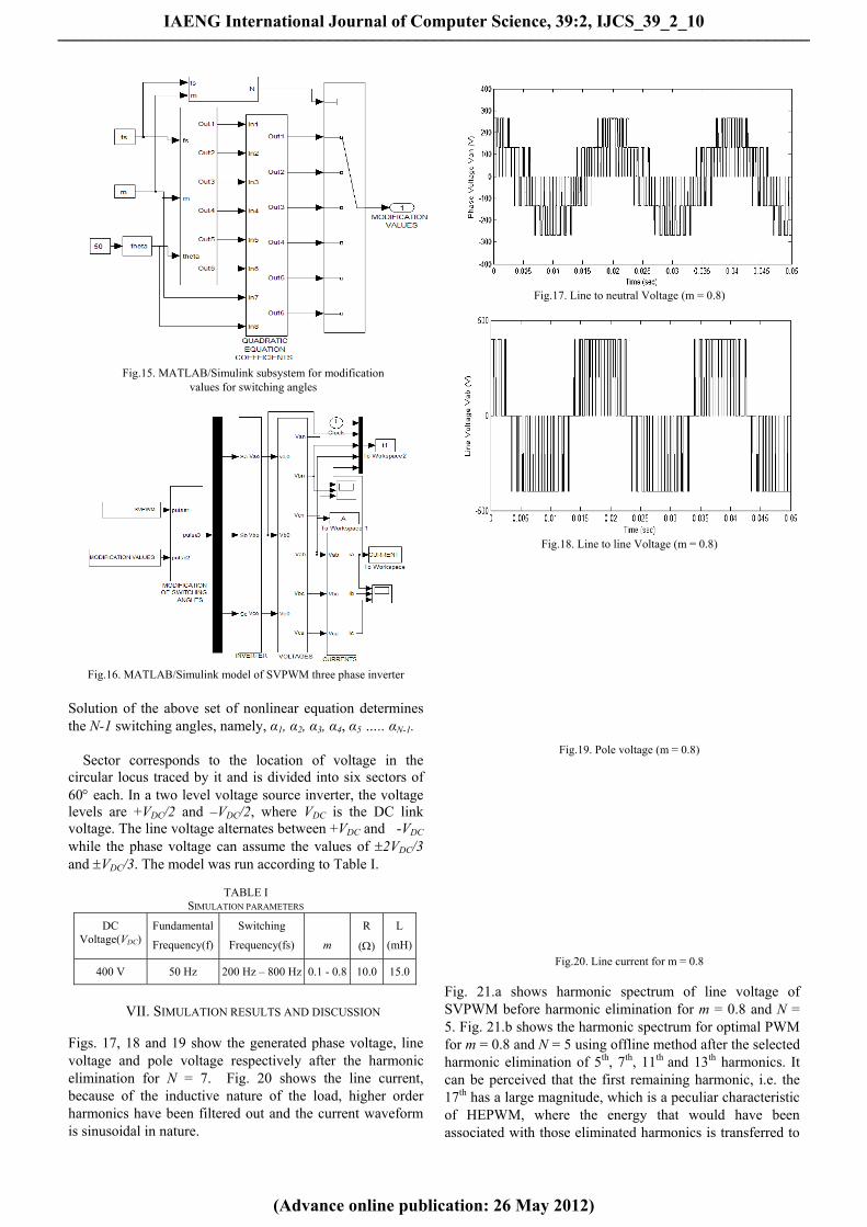
Fig.15. MATLAB/Simulink subsystem for modification

values for switching angles

Fig.16. MATLAB/Simulink model of SVPWM three phase inverter

Solution of the above set of nonlinear equation determines the N-1 switching angles, namely, α1, α2, α3, α4, α5 ….. αN-1. Sector corresponds to the location of voltage in the circular locus traced by it and is divided into six sectors of 60 each. In a two level voltage source inverter, the voltage levels are +VDC/2 and –VDC/2, where VDC is the DC link voltage. The line voltage alternates between +VDC and -VDC while the phase voltage can assume the values of 2VDC/3 and VDC/3. The model was run according to Table I.

TABLE I

SIMULATION PARAMETERS

DC Voltage(VDC)

Fundamental

Frequency(f)

Switching

Frequency(fs)

m

R

()

L

(mH)

400 V 50 Hz 200 Hz – 800 Hz 0.1 - 0.8 10.0 15.0

VII. SIMULATION RESULTS AND DISCUSSION

Figs. 17, 18 and 19 show the generated phase voltage, line voltage and pole voltage respectively after the harmonic elimination for N = 7. Fig. 20 shows the line current, because of the inductive nature of the load, higher order harmonics have been filtered out and the current waveform is sinusoidal in nature.

Fig.17. Line to neutral Voltage (m = 0.8)

Fig.18. Line to line Voltage (m = 0.8)

Fig.19. Pole voltage (m = 0.8)

Fig.20. Line current for m = 0.8

Fig. 21.a shows harmonic spectrum of line voltage of SVPWM before harmonic elimination for m = 0.8 and N = 5. Fig. 21.b shows the harmonic spectrum for optimal PWM for m = 0.8 and N = 5 using offline method after the selected harmonic elimination of 5th, 7th, 11th and 13th harmonics. It can be perceived that the first remaining harmonic, i.e. the 17th has a large magnitude, which is a peculiar characteristic of HEPWM, where the energy that would have been associated with those eliminated harmonics is transferred to



______________________________________________________________________________________

the first remaining harmonic [31]. Fig. 21.c shows harmonic spectrum of line voltage using online method by the proposed model for the same parametric values. It can be observed that all the selected harmonics are effectively eliminated. This ensures the accuracy of the model in eliminating low order harmonics when comparing with the offline method. Table II gives the normalized magnitudes of line voltage for m = 0.2, m = 0.4 and m = 0.8 with N = 5, which shows that harmonic performance is more or less uniform in the modulation index ranging from 0.1 to 0.9. Fig. 22.a shows harmonic spectrum of line voltage of SVPWM before harmonic elimination for m = 0.8 and N = 7. Fig. 22.b shows the harmonic spectrum for SHEPWM for m = 0.8 and N = 7 using offline method after the selected harmonic elimination of 5th, 7th, 11th, 13th, 17th and 19th harmonics, while Fig. 21.c shows harmonic spectrum of line voltage using online method by the proposed model for the same parametric values. Table III shows the normalized magnitudes of line voltage for m = 0.2, m = 0.4 and m = 0.8 with N = 7, which ensures the uniformity of harmonic performance in the modulation index ranging from 0.1 to 0.9.

a. SVPWM

b. HEPWM by offline method

c. HEPWM by online method

Fig. 21 Harmonic spectrum for Line Voltage (N = 5)

TABLE II.

NORMALISED MAGNITUDE OF LINE VOLTAGE FOR N = 5

Harmonicorder

Modulation index m = 0.2 m = 0.4 m = 0.8

SV PWM

HEPWM SV PWM

HEPWM SV PWM

HEPWM offline online offline online offline online

1 1.00 1.00 1.00 1.00 1.00 1.00 1.00 1.00 1.005 0.00 0.00 0.01 0.03 0.00 0.00 0.16 0.00 0.007 0.04 0.00 0.02 0.08 0.00 0.01 0.16 0.00 0.0111 0.87 0.00 0.03 0.68 0.00 0.01 0.18 0.00 0.0113 0.16 0.00 0.00 0.27 0.00 0.00 0.10 0.00 0.0217 0.13 0.82 0.82 0.18 0.38 0.39 0.05 0.30 0.3219 0.93 0.85 0.86 0.52 0.51 0.51 0.14 0.06 0.0523 0.23 0.10 0.12 0.25 0.28 0.27 0.21 0.14 0.1025 0.12 0.07 0.07 0.29 0.17 0.17 0.10 0.06 0.0629 0.75 0.06 0.08 0.04 0.11 0.12 0.14 0.07 0.0531 0.41 0.09 0.08 0.12 0.15 0.15 0.02 0.05 0.0735 0.20 0.42 0.43 0.25 0.22 0.22 0.04 0.10 0.1237 0.18 0.47 0.49 0.10 0.11 0.11 0.08 0.08 0.0741 0.17 0.22 0.23 0.15 0.10 0.11 0.11 0.02 0.0843 0.24 0.15 0.13 0.08 0.11 0.12 0.06 0.05 0.0647 0.14 0.13 0.11 0.22 0.06 0.07 0.07 0.14 0.1149 0.25 0.17 0.17 0.17 0.2 0.01 0.02 0.06 0.05

a. SVPWM

b. HEPWM by offline method

c. HEPWM by online method

Fig. 22. Harmonic spectrum for Line Voltage (N = 7)

0.0

0.2

0.4

0.6

0.8

1.0

0 1 5 7 11 13 17 19 23 25 29 31 35 37 41 43 47 49

Nor

mal

ised

mag

nitu

de

Harmonic order

N = 5m=0.8

WTHD=4.53%

0.0

0.2

0.4

0.6

0.8

1.0

0 1 5 7 11 13 17 19 23 25 29 31 35 37 41 43 47 49

Nor

mal

ised

mag

nitu

de

Harmonic order

N = 5m=0.8

WTHD=1.99%

0.0

0.2

0.4

0.6

0.8

1.0

0 1 5 7 11 13 17 19 23 25 29 31 35 37 41 43 47 49

Nor

mal

ised

mag

nitu

de

Harmonic order

N = 5m=0.8

WTHD=2.03%

0.0

0.2

0.4

0.6

0.8

1.0

0 1 5 7 11 13 17 19 23 25 29 31 35 37 41 43 47 49

Nor

mal

ised

mag

nitu

de

Harmonic order

N = 7m = 0.8

WTHD=4.86%

0.0

0.2

0.4

0.6

0.8

1.0

0 1 5 7 11 13 17 19 23 25 29 31 35 37 41 43 47 49

Nor

mal

ised

mag

nitu

de

Harmonic order

N = 7m = 0.8

WTHD=1.33%

0.0

0.2

0.4

0.6

0.8

1.0

0 1 5 7 11 13 17 19 23 25 29 31 35 37 41 43 47 49

Nor

mal

ised

mag

nitu

de

Harmonic order

N = 7m = 0.8

WTHD=1.36%



______________________________________________________________________________________

TABLE III. NORMALISED MAGNITUDE OF LINE VOLTAGE FOR N = 7

Harmonic order

Modulation index m = 0.2 m = 0.4 m = 0.8

SV PWM

HEPWM SV PWM

HEPWM SV PWM

HEPWM offline online offline online offline online

1 1.00 1.00 1.00 1.00 1.00 1.00 1.00 1.00 1.005 0.20 0.00 0.04 0.16 0.00 0.01 0.20 0.00 0.027 0.18 0.00 0.03 0.04 0.00 0.01 0.02 0.00 0.0311 0.32 0.00 0.05 0.23 0.00 0.00 0.15 0.00 0.0213 0.81 0.00 0.05 0.68 0.00 0.00 0.23 0.00 0.0417 0.19 0.00 0.06 0.31 0.00 0.01 0.16 0.00 0.0119 0.19 0.00 0.06 0.21 0.00 0.01 0.19 0.00 0.0123 0.06 0.84 0.83 0.13 0.40 0.41 0.11 0.27 0.2225 0.45 0.90 0.89 0.22 0.61 0.59 0.03 0.01 0.0529 0.89 0.03 0.04 0.40 0.17 0.15 0.12 0.03 0.0331 0.40 0.11 0.11 0.32 0.25 0.27 0.17 0.14 0.1635 .03 0.05 0.03 0.10 0.06 0.06 0.01 0.07 0.1037 0.7 0.06 0.04 0.16 0.13 0.14 0.05 0.04 0.0341 0.27 0.08 0.06 0.07 0.15 0.18 0.05 0.04 0.0843 0.63 0.01 0.06 0.01 0.00 0.03 0.14 0.07 0.0747 0.27 0.50 0.35 0.17 0.14 0.08 0.01 0.14 0.1349 0.06 0.59 0.54 0.11 0.05 0.05 0.02 0.06 0.02

The variation of WTHD in line voltage as a function of modulation index for SVPWM and HEPWM by offline method are shown in Figs. 23 and 24 for N = 5 and N = 7 respectively. These curves show that a marginal improvement of WTHD is possible for the modulation index ranging from 0.1 to 0.9. Figs. 23 and 24 also reveal that the graphs for HEPWM by offline and online methods are coinciding in almost all the ranges of modulation indices. Table IV shows WTHD for m = 0.2, m = 0.4 and m = 0.8 with N = 5 and N = 7. These results ensure the effectiveness of the proposed model in generating a high quality PWM waveform. Similar results are generated for N = 2, 3, …., which are not included in this paper. It is examined that the model can perform precisely for a wide range of switching frequency from 200 Hz onwards.

TABLE IV COMPARISON OF WTHD

N

m = 0.2 m = 0.4 m = 0.8

SV PWM

HEPWM SV PWM

HEPWM SV PWM

HEPWM

offline online offline online offline online

5 10.0% 6.89% 6.95% 7.51% 3.89% 3.94% 4.53% 1.99% 2.03%

7 9.50% 5.34% 5.36% 7.10% 3.19% 3.20% 4.90% 1.33% 1.36%

Fig. 23. Line voltage WTHD Vs Modulation index for N = 5

Fig. 24. Line voltage WTHD Vs Modulation index for N = 7

V. CONCLUSIONS

This paper proposed a new procedure for an efficient and fast online method for the harmonic elimination of SVPWM for three phase inverter. The SVPWM output waveform is modified for an optimal PWM waveform by applying modification values to the switching angle pattern of SVPWM, which are calculated online using polynomial equations. These polynomial equations are functions of modulation index and the coefficients are determined using curve fitting technique. Output waveforms of MATLAB/Simulink model for SVPWM three phase inverter is generated. Harmonic performance of the modified output waveform is carried out by comparing the WTHD of the same with that of offline method.

The simulation results show that the proposed online

method is precise as offline method in eliminating the low order harmonics and reducing the total harmonic distortion (using WTHD). Comparing with other conventional online methods, in the proposed method there is no need to save all the optimal switching angles in the form of look-up tables. Instead, only the coefficients of quadratic functions are saved in the memory, which requires less memory space. The online computation of the quadratic polynomial functions are simple which need only the addition and multiplication processes, allowing its practical implementation using low cost microprocessors and DSPs. The developed model allows the user to control the voltage in a wide range or the number of switching angles by varying the switching frequency according to their design requirements. Considering the accuracy and effectiveness, the proposed inverter model has considerable practical use for variable-speed AC motor drive applications, where harmonics in the output of the inverter pose serious problems in the motor performance. The model can be adapted for applications like UPS with fixed frequency or in application where the inverter has to track the grid.

0.00

2.00

4.00

6.00

8.00

10.00

12.00

0.1 0.2 0.3 0.4 0.5 0.6 0.7 0.8 0.9

HEPWM(offline)HEPWM (online)SVPWM

WT

HD

(%

)

Modulation index

0.00

2.00

4.00

6.00

8.00

10.00

12.00

14.00

0.1 0.2 0.3 0.4 0.5 0.6 0.7 0.8 0.9

HEPWM(offline)

HEPWM(online)

SVPWM

WT

HD

(%

)

Modulation index



______________________________________________________________________________________

ACKNOWLEDGEMENT

The first author acknowledges support from SPEED-IT Research Fellowship from IT Department of the Government of Kerala, India.

REFERENCES

[1] B. K. Bose, “Adjustable speed AC drives - A technology status review,” Proceedings of the IEEE- IECON, Vol. 70, pp. 116-135, February 1982.

[2] D. G. Holmes and T. A. Lipo, “Pulse Width Modulation for Power Converters: Principles and Practice,” New Jersey: Wiley IEEE Press, 2003.

[3] J. Holtz, P. Lammert and W. Lotzkat, “High speed drive system with ultrasonic MOSFET PWM inverter and single-chip microprocessor control,” IEEE Transactions on Industry Applications, Vol. 23, No.6 pp. 1010-1015, November 1987.

[4] J. Holtz, “Pulse width modulation - a survey,” IEEE Transactions on Industrial Electronics, Vol. 39, No. 5, pp. 410-420, October 1992.

[5] H. W. Van der Broeck, H. C. Skudelny and G.V. Stanke," Analysis and realisation of a pulse width modulator based on voltage space vectors", IEEE Transactions on Industry Applications, Vol. 24, pp. 142-150, January/February 1988.

[6] A. Mehrizi-Sani and S. Filizadeh, “Digital Implementation and Transient Simulation of Space Vector Modulated Converters,” IEEE Power Engineering Society General Meeting, Montreal, QC, Canada, June 2006.

[7] Fang Zheng Peng, Jih-Sheng Lai, et. al, “A Multilevel Voltage- Source Inverter with Separate DC Sources for Static Var Generation,” IEEE Transactions on Industry Applications, Vol. 32, No. 5, pp. 1130-1138, September/October 1996.

[8] Jose Rodriguez, J. S. Lai, and F. Z. Peng, “Multilevel Inverters: A Survey of Topologies, Controls, and Applications,” IEEE Transactions on Industrial Electronics, Vol. 49, No. 4, pp. 724-738, August 2002.

[9] O. Lopez, J. Alvarez, J. Doval-Gandoy, and F. D. Freijedo, “Multilevel multiphase space vector PWM algorithm,” IEEE Transactions on Industrial Electronics, Vol. 55, No. 5, pp. 244-251, May 2008.

[10] J. F. Moynihan, M. G. Egan and J. M. D. Murphy,” Theoretical spectra of space vector modulated waveforms,” IEE Proc. Electrical Power Applications, Vol. 145, No. 1, January 1998.

[11] J. W. Chen and T. J. Liang, “A Novel Algorithm in Solving Nonlinear Equations for Programmed PWM Inverter to Eliminate Harmonics,” 23rd International Conference on Industrial Electronics, control and Instrumentation IEEE IECON ‘97, Vol. 2, pp. 698-703, November 1997.

[12] J. N. Chiasson, L. M. Tolbert, K. J. McKenzie and Z. Du, “Elimination of harmonics in a multilevel converter using the theory of symmetric polynomials resultants,” IEEE Transactions on Control System Technology, Vol. 13, No. 2, pp. 216-223, March 2005.

[13] B. Ozpineci, L. M. Tolbert and J. N. Chiasson, “Harmonic optimization of multilevel converters using genetic algorithms, IEEE Power Electronics Letters, Vol. 3, No. 3, pp. 92-95, September 2005.

[14] H. S. Patel and R. G. Hoft, ’’Genealized techniques of harmonic elimination and voltage control in thyristor inverters: Part I- Harmonic elimination,” IEEE Transactions on Industry Applications, Vol. 9, No. 3, pp. 310-317, May/June 1973.

[15] Q. Jiang, D. Grahame Holmes, David B. Giesner, “A Method for Linearising Optimal PWM Switching Strategies to Enable their Computation On-line in Real-time,” Conference Proceedings of the IEEE Industry Applications Society Annual Meeting ’91, Vol. 1, pp. 819-825, September/October 1991.

[16] Taufiq, J. A., Mellitt, B and Goodman, C. J., “Novel Algorithm for Generating Near Optimal PWM waveforms for AC Traction Drives”, IEE Proceedings B on Electric Power Applications, Vol. 133, No. 2, pp. 85-94,March 1986.

[17] S. R. Bowes, ”Advanced Regular Sampled PWM control techniques for drives and static power converters,” IEEE Transactions on Industrial Electronics, Vol. 42, No. 4, pp. 367-373, August 1995.

[18] S. R. Bowes, ”Novel space vector based harmonic elimination inverter control,” IEEE Transactions on Industry applications, Vol. 36, No. 2, pp. 549-557, March/April 2000.

[19] J. N. Chiasson, L. M. Tolbert, K. J. McKenzie and Z. Du, “A complete solution to the Harmonic Elimination Problem,” IEEE Transactions on Power Electronics, Vol. 19, No. 2, pp. 3-9, March 2004.

[20] Nguyen Van Nho and Myung Joong Youn, ” A Simple Online SHEPWM with Extension to Six Step Mode in Two Level Inverters,” IEEE International Conference on Power Electronics and drive Systems-PEDS’05, Vol. 2, pp. 1419-1424, November 2005.

[21] A. I., Maswood, “PWM SHE Switching Algorithm for Voltage Source Inverter,”IEEE International Conference on Power Electronics, Drives and Energy Systems-PEDES’06, pp. 1-4, December 2006.

[22] Yu Liu, Hoon Hong and Alex Q. Huang, “Real-time Calculation of Switching Angles Minimizing THD for Multilevel Inverters with Step Modulation,” IEEE Transactions on Industrial Electronics, Vol. 56, No. 2, pp. 285-293, February 2009.

[23] Zhi Zeying Liu Hui and Han Rucheng. “CFT based on-line calculation for Optimal PWM switching angles”, IEEE Conference on Power and Energy Engineering – APPEEC’09, pp. 1-5, March 2009.

[24] N. Ahmed Azli and A. H. M. Yatim, “A Curve Fitting Technique (CFT) for Optimal PWM Online Control of a Modular Structured Multilevel Inverter (MSMI)”, 4th IEEE International conference on Power Electronics and Drive Systems, Vol. 2, pp. 598-604, October 2001.

[25] N. Azli, A. H. M. Yatim, “Curve fitting technique for optimal pulsewidth modulation(PWM)online control of a voltage source inverter (VSI)”, Proceedings of TENCON 2000,Vol. 1, pp. 419-422.September 2000.

[26] V. G. Agelidis, A. I. Balouktsis, and M. S. A. Dahidah, “A five level symmetrically defined selective harmonic elimination PWM strategy: Analysis and experimental validation,” IEEE Transactions on Power Electronics, vol. 23, no. 1, pp. 19-26, January 2008.

[27] G. K. Nisha, S. Ushakumari and Z. V. Lakaparampil, “Harmonic Elimination of Space Vector Modulated Three Phase Inverter”, Lecture Notes in Engineering and Computer Science: Proceedings of the International Multi-conference of Engineers and Computer Scientists 2012, IMECS 2012, 14-16 March, 2012, Hong Kong, pp. 1109-1115.

[28] G. K. Nisha, S. Ushakumari and Z. V. Lakaparampil, “Method to Eliminate Harmonics in PWM: A Study for Single Phase and Three Phase”, International conference on Emerging Technology, Trends on Advanced Engineering Research, Vol. 2, pp. 598-604, February 2012.

[29] A. Mehrizi-Sani and S. Filizadeh, “An optimized Space Vector Modulation Sequence for Improved Harmonic Performance,” IEEE Transactions on Industrial Electronics, Vol. 56, No. 8, pp. 2894-2903, August 2009.

[30] IEEE Recommended Practices and Requirements for Harmonic Control in Electrical Power Systems, IEEE Standard 519, 1992.

[31] S. R. Bowes and D. Holliday, ”Optimal Regular Sampled PWM inverter control techniques,” IEEE Transactions on Industrial Electronics, Vol. 54, pp. 1547-1559, June 2007.

Nisha G.K. (M’12) was born in Trivandrum, India on 20th May 1976. She received the B.Tech. degree in Electrical and Electronics Engineering from TKM College of Engineering (University of Kerala) and M.Tech. degree in Electrical Machines from Government College of Engineering, Trivandrum (University of Kerala), Kerala, India, in 1997 and 2000 respectively. She is currently a Research Scholar in Government College of Engineering (University

of Kerala), Trivandrum, India. From 2001 to 2010, she was with the University College of Engineering, Trivandrum as Lecturer and with the Mar Baselios College of Engineering and Technology, Trivandrum as Assistant Professor in the Department of Electrical Engineering. Her research interest includes ac drives, pulse width modulation and field oriented control. Ms. Nisha received Certificate of Merit (student) Award for the 2012 IAENG International Conference on Electrical Engineering.



______________________________________________________________________________________

Dr. S. Ushakumari was born in Kollam, India on 15th May 1963. She received her B.Tech. Degree in Electrical Engineering from TKM college of Engineering (University of Kerala), Kollam, Kerala, India in 1985, M.Tech. in 1995 and Ph.D. in 2002 in the area of Control systems from Government College of Engineering (University of Kerala), Trivandrum, Kerala, India. She joined in the Department of Electrical Engineering, Government College of Engineering,

Trivandrum, Kerala, India in 1990, where she is currently an Associate Professor from 2002 onwards. She has 9 publications in international journals and 32 national and international conferences at her credit. Area of interest includes robust and adaptive control systems, drives, fuzzy logic, neural network etc. Presently guiding 5 research candidates in the area of control and drives systems. She is a reviewer of IEEE Transactions on Industrial Electronics, Elsevier International journal on Computers and Electrical Engineering and AMSE international journal on modeling and simulation. Presently coordinates 3 research projects and editor of the international journal on Electrical Sciences being published. Dr. Ushakumari is a life member of ISTE and secretary of ISTE Trivandrum chapter.

Dr. Z.V. Lakaparampil was born in Changanacherry, Kerala, India on 17th October 1956. He received BSc(Engg.) in Electrical Engineering from NIT Calicut, Kerala, India, in 1979, and DIISc in Electronics Design Technology and PhD in Electrical Engineering from Indian Institute of Science, Bangalore, India in 1980 and 1995 respectively. He is currently an Associate Director in Centre for Development of Advanced Computing (C-

DAC), Trivandrum, Kerala, India. From 1979 to 1988, he was with Keltron, Kerala, India. Since then he is with CDAC-T, His area of specialization are embedded controllers for power electronics, vector/ field oriented control, real-time simulator etc. He has 3 publications, 30 international/national papers, 2 patents and one copyright to his credit. PhD guide for 4 research scholars from different Universities. Dr. Lakaparampil is a Member of IEEE, life member of Institution of Engineers (India), Member of Engineering and Technology Programmes KSCSTE, Government of Kerala, India and Member for EV/HEV panel for Collaborative Automotive Research.



______________________________________________________________________________________

online harmonic elimination of svpwm for three phase ... · pdf fileonline harmonic...

Documents