On the satellite altimeter crossover problemH. van Gysen1, R. Coleman2,3

1Department of Surveying and Mapping, University of Natal, King George V Avenue, Durban. 4001. South Africa2Department of Surveying and Spatial Information Science, University of Tasmania, GPO Box 252-76, Hobart. 7001. TAS. Australia3CSIRO Division of Oceanography, GPO Box 1538, Hobart. 7001. TAS. Australia

Received 11 September 1995; Accepted 2 September 1996

Abstract. Mean sea surface heights and residual radialorbit errors are estimated simultaneously in a singleglobal crossover adjustment of multiple cycles ofsatellite altimetry data. The rank defect inherent in theestimation problem is explicitly identified and treated invarious ways to give solutions that minimise (in norm)either orbit errors or mean sea surface heights. The rankdefect gives rise to geographically correlated orbit error,consisting of those components of the orbit error orthose components of the map of sea surface heightswhich fall within the nullspace of the estimation problemand which cannot be distinguished as orbit error orocean signal. We show that, in the case of TOPEXOPEX/POSEIDONOSEIDON data, the geographically correlated errorconsists largely of long-wavelength and long-period seasurface fluctuations, which in the past has often beenassigned as orbit error.

1. Introduction

The Topex/Poseidon (T/P) satellite altimeter missionsaw a quantum improvement in the accuracy ofaltimeter sea surface heights (SSHs) due, in largemeasure, to improved orbits. T/P has an orbit errorbudgeted to be 13 cm (TOPEXOPEX/POSEIDONOSEIDON Project, 1992),and reported in reality to be better than 5 cm (Le Traonet al., 1994; Tapley et al., 1994), in contrast to Geosatorbits, which were initially good to 3 metres andimproved to about 20–50 cm for the precise orbitsbased on the GEM-T2 geopotential model (Shum et al.,1990; Haines et al., 1994).

With such good orbits and consequently such goodmeasured SSHs, it is argued in some quarters it doesmore harm than good to use any of the empirical,nondynamical orbit error reduction techniques that havebecome a traditional part of satellite altimetry data

processing (Stammer and Wunsch, 1994). Of particularconcern are the indications that orbit error removal alsoremoves long-wavelength, basin-scale and larger, oceansignals (Tai, 1991; Miller et al., 1993; Tai and Wagner,1994; Wagner and Tai, 1995). We show here that thisconcern is well founded, and that supposed orbit errors,certainly in the case of T/P orbits, in reality containlong-wavelength, small-amplitude ocean signals.

On the other hand, the reduction of noise levels inSSHs allows other signals to be unmasked, such asplanetary waves, shortcomings in present tide models,and annual and longer period changes in mean sea level(MSL). It is our view that if these long-wavelength,small-amplitude effects are to be uncovered, care is stillneeded in the reduction and processing of altimetry data.The main requirement is to estimate mean sea level in aconsistent and uniform way since everything else flowsfrom this mean – mesoscale variability, seasonal varia-tions in sea surface height (SSH), trend in mean sea level(Wagner and Cheney, 1992) – while taking into accountthe radial orbit error, including the geographicallycorrelated component of the error. Further, in theprocessing of ERS-1/2 data and in the reprocessing ofGeosat data, improved gravity field models notwith-standing, there is still a need to take residual radial orbiterrors into account.

In this paper we present a model for doing a globalcrossover adjustment in which the mean sea surfaceheights are estimated directly, and not removed at theoutset through crossover differences, as is usually done.Also part of the model is an estimation of the radialcomponent of the orbit error, for which any of themodels which have gained acceptance in the last fewyears can be used. We will concentrate on an orbit errormodel (in equation (1) below) that derives from theanalytical studies by Colombo (1984), Wagner (1985),Rosborough (1986), Engelis (1988), Moore andRothwell (1990), and others, which takes into accounterrors in the geopotential, errors in the modelling ofdrag and solar radiation forces on the satellite, anderrors in the initial state vector.Correspondence to: H. van Gysen

Journal of Geodesy (1997) 71: 83–96

Whatever model is chosen to represent the orbiterror, it will have associated with it a null surface which,on the basis of the given altimeter measurements alone,cannot be included in the mean sea surface or assignedto the orbit error. This is the geographically correlatederror (GCE) falling within the nullspace of the estima-tion problem; the dimension of the surface equals thedimension of the nullspace (Schrama, 1989; 1992). Thetreatment of this rank defect requires special attention.It can be determined (in whole, or perhaps only in part)by outside measurements or by outside constraints, forexample, in the comparison of the T/P orbits (based onthe JGM-2 gravity field) with orbits obtained using theT/P GPS Demonstration receiver (Bertiger et al., 1994),and in the T/P verification measurements at PlatformHarvest, Lampione and Bass Strait (Christensen et al.,1994; Menard et al., 1994; White et al., 1994). In theabsence of any external reference, the singularity of theestimation problem needs to be overcome in some otherway. This has often been done in an ad hoc fashion, byusing master arcs, or by putting extra weight on thediagonal (ridging) of the normal equation matrix of thecrossover difference problem (Rapp, 1979; Douglas etal., 1984; Tai, 1988; Houry et al., 1994). Alternateapproaches have been suggested by, for example,Wunsch and Zlotnicki (1984) and Blanc et al. (1995)using inverse formalism. However, this latter technique,while making a much better attempt to separate oceansignal from radial orbit error and altimeter measurementnoise, remains sub-optimal as global analyses cannot beattempted due to the computational burden of theproblem.

In our approach we have addressed the followingissues: (i) to make global solutions computationallytractable, (ii) using a well-established analytical form forthe description of the radial orbit error model, the exactnature of the rank defect of the problem can beformulated, (iii) a conscious choice can then be madeas to where to ‘place’ the nullspace of the solution.

The choice of nullspace definition can be guided bybackground knowledge of the ocean signal and the likelymagnitudes of mean orbit errors, but in this definitionthere can be no absolute certainty about where the GCEbelongs. If one believes the GCE indeed to be orbiterror, a solution can be found for the mean SSHs whichcontains nothing that looks like orbit error. At the otherextreme, if one believes that the orbits are free of GCE, asolution can be found in which the overall change to theorbits is zero and the GCE signature is placed in theSSHs. It is also possible to obtain solutions whichdistribute the nullspace between orbits and SSHs insome predetermined proportion, or which assign certaincomponents of the nullspace to SSHs and the remainderas a correction to the orbits overall.

If the choice as to what to do with the GCE isultimately arbitrary, it should also be mentioned that allthe possibilities suggested above will be ‘minimumconstraint’ solutions for which the measurement resi-duals will be invariant. Thus, for studies in which theresiduals are used – for SSH variability, seasonalvariability, long-term trends – it does not matter which

solution is chosen. It does matter, however, if the SSHsthemselves are used, to determine general ocean circula-tion, for example.

The advantages we see for our approach are thefollowing:

– By working directly with SSHs, and not with cross-over differences, there is no need to assume aninvariant sea level change over the interval makingup the crossover pair, i.e., no time criterion for aminimum crossover time between pairs of tracks needbe applied.

– The mean sea surface is an explicit average over thenumber of repeat data in the adjustment, with allcycles contributing simultaneously; moreover, theestimation of mean SSH is simultaneous with estima-tion of the orbit error parameters.

– The nullspace of the estimation problem is explicitlycharacterised, and is accounted for (taken up in theorbits or in the mean SSHs) in a deliberate way.

– And finally, the solution presented here is computa-tionally tractable, making possible crossover solu-tions for full or multiple altimetric missions.

2. Theory

2.1 Orbit Model

Suppose a satellite to be in a repeating, near-circularorbit, with orbital period T0 and Te the length of a nodalday (the rotation period of the earth with respect to thesatellite’s orbital plane); then NRT0 � NDTe for integersNR and ND relatively prime to each other. (The satellitethus completes NR orbits in ND whole nodal days; for T/P, NR � 127, ND � 10).

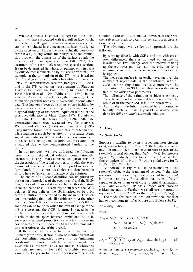
As indicated in Figure 1, i is the inclination of thesatellite’s orbit, x the argument of perigee, X the rightascension of the ascending node, h sidereal time, and Mis the mean anomaly. For satellites that are in a ‘frozen’repeat orbit, or in an orbit close to critical inclination,_x � 0 and x � p=2. T/P has a frozen orbit close to

critical inclination. Further, we shall use the notationx0 � x � M ; xe � X ÿ h (so that _xe= _x0 � ÿND=NR).

The model for the radial orbit error we shall considerhas two components (after Moore and Ehlers (1993)):

Dr � Drng � Drg ; �1�

where

Drng � D1�t ÿ t0� � D2�t ÿ t0� sin M

� D3�t ÿ t0� cos M � D4�t ÿ t0� sin 2M

� D5�t ÿ t0� cos 2M �2�

Drg �Xlmax

l�0

Xl

m�0

Xl

p�0

�Almp cos wlmp � Blmp sin wlmp � ; �3�

where t is time, t0 is a reference epoch, wlmp = �l ÿ 2p �x0�mxe �

_wlmp t � _x0�l ÿ 2p ÿ mND=NR�t, and Almp ;

84

Blmp ; Dk are coefficients. The Drng term takes intoaccount error contributions that are mostly nongravita-tional, such as initial state vector and surface forcemodelling (Moore and Rothwell, 1990; Moore andEhlers, 1993), and Drg contains errors due to the gravityfield. Notice that the bias term is the first term in thesummation for Drg.

The ‘gravitational’ frequencies _wlmp in equation (3)account for errors in the gravitational field; the primaryterm is at one cycle/rev, the other terms are harmonics ofthis fundamental frequency, _x0, and combinations of _x0with the nodal frequency _xe. These are the dominantfrequencies predicted by analytical perturbation theoryand are shown up by spectral analysis of orbit errors(see, for example Fu and Vazquez (1988); Chelton andSchlax (1993), Houry et al. (1994), among many suchstudies).

The terms in equation (3) are related to surfacespherical harmonics by Kaula’s transformation (Kaula,1966):

rclm

rslm

� �

�

ClmPlm�sin /� cos mk

SlmPlm�sin /� sin mk

� �

�

ClmPl

p�0 Flmp �i�cos wlmp

sin wlmp

" #lÿm even

lÿm odd

SlmPl

p�0 Flmp �i�sin wlmp

ÿ cos wlmp

" #lÿm even

lÿm odd

2

666664

3

777775

�4�

where / is geocentric latitude, k is longitude, Plm areassociated Legendre functions and the Flmp �i� are theinclination functions given by Kaula (1966).

When we sum

Drg �Xlmax

l�0

Xl

m�0

�rclm � rs

lm� �5�

with

Almp

Blmp

� �

� Flmp �i�

Clm

ÿSlm

� �lÿm even

lÿm odd

Slm

Clm

� �lÿm even

lÿm odd

2

6664

3

7775

; �6�

we see that the expression for the ‘gravitational’component of the radial error is transformed from thetime domain to the spatial or geographical domain.Each spherical harmonic rc

lm; rslm with l � lmax can be

expressed as a linear combination l orbital frequencies(plus a possible ‘zero’ frequency). For lmax � 2, theselinear combinations are (see also Schrama (1989)):

rc00 � C00F000

rc10 � C10�F100 ÿ F101� sin x0

rc11 � C11�F110 cos�x0 � xe� � F111 cos�x0 ÿ xe��

rs11 � S11�F110 sin�x0 � xe� ÿ F111 sin�x0 ÿ xe��

rc20 � C20�F201 � �F200 � F202� cos 2x0�

rc21 � C21�F210 sin�2x0 � xe� � F211 sin xe

ÿ F212 sin�2x0 ÿ xe��

rs21 � S21�ÿF210 cos�2x0 � xe� ÿ F211 cos xe

ÿ F212 cos�2x0 ÿ xe��

rc22 � C22�F220 cos�2x0 � 2xe� � F221 cos 2xe

� F222 cos�2x0 ÿ 2xe��

rs22 � S22�F220 sin�2x0 � 2xe� � F221 sin 2xe

ÿ F222 sin�2x0 ÿ 2xe�� :

�7�

These linear combinations, the ‘geographic correlations’,are what give rise to the GCE and the singularity in thecrossover adjustment problem. The nature of thesesingularities is discussed further in section 2.3 below.

Fig. 1. Relation between orbital elements: iis inclination of the orbit, x argument ofperigee, X right ascension of the ascendingnode, h sidereal time, M mean anomaly

85

2.2 Altimetric Equation

Let crossover points (crossovers of ascending anddescending passes within a single ND-day repeat cycle)be numbered or ordered in some way; we will use theabsence or presence of primes to distinguish betweenascending and descending passes. At the ith crossoverpoint the altimetric equation relating altimeter measure-ment and sea surface height is (for the ascending pass):

li � hi � Aix � �i ; �8�

where li � rellipsoid ÿ raltimeter is the difference between theheight (range) of the satellite above the referenceellipsoid and the measured range to the instantaneoussea surface, with the altimeter range corrected in theusual way for such effects as earth and ocean tides,atmospheric pressure, significant wave height andpropagation delays; hi is the instantaneous SSH abovethe ellipsoid at the crossover point; Aix the orbitalcorrection term, and �i is measurement noise. Theinstantaneous SSH can be split as

hi � hi � finstant; i � Ni � fpermanent; i � finstant; i ; �9�

where hi is the mean SSH (� Ni, the geoid height plusfpermanent; i, the permanent or stationary component ofthe sea surface topography (SST)), and finstant; i is theinstantaneous or variable component of SST.

The hi term is used since it is not possible to separateNi and fpermanent; i unless we have additional informationor use some form of external constraints. Somepossibilities are: (1) use inverse formalisms such as thoseoriginally proposed by Wunsch and Gaposchkin (1980);(2) use simultaneous, in-situ hydrographic measure-ments in the set of crossover observation equations (vanGysen et al. (1995)) or forms of oceanographicconstraint equations in closed areas, such as conserva-tion of horizontal divergence – for example, Mesais andStrub (1995)); (3) adopt a model for fpermanent; i and thussolve for Ni – this gives us no new oceanographicinformation, only a geoid that is as good as thedefinition of fpermanent; i; (4) wait for the launch of adedicated geopotential research satellite mission. Toobtain new oceanographic results, the last two optionsare not viable possibilities and so we adopt a pragmaticview towards a solution and use our proposed crossovertechnique.

We will combine finstant; i and �i into a single ‘error’term, vi, so that our observation model becomes

li � hi � Aix � vi : �10�

The vi term thus contains both measurement error andthe time-varying, instantaneous component of SST. Themeasurement equation for the descending pass at thesame point reads

l0i � hi � A0

ix � v0i : �11�

At this point it is customary to form crossoverdifferences, li ÿ l0i, in which the mean SSH, hi, no longerappears. However, our approach is to continue with the

measurement model above, in which both mean SSHand orbit correction terms appear.

Suppose there are a total of n crossovers; putting nascending measurements li and n descending measure-ments l0i together, we have

l � h � Ax � v

l0 � h � A0x � v0�12�

where l; l0; v; v0 and h are n-vectors, x is a u-vector of(unknown) orbit model coefficients, and A; A0 are �n; u�-matrices of observation equation coefficients. Weassume all 2n measurements are of equal precision anduncorrelated. This is a considerable presumption, sincethe errors v and v0 also contain SSH variations, whichare markedly inhomogeneous and can be significantlycorrelated, both spatially and temporally.

From these 2n measurements we seek to estimate then heights in h and u orbit parameters in x; for this weshall use least squares. However, a problem to be facedis that the estimation problem in equation (12) issingular, because of the GCE. It is to the identificationand regularisation of this singularity that we now turn.

2.3 Singularity

Another way of writing equation (12) is as

ll0

� �

� X hx

� �

�

vv0

� �

; �13�

where

X�2n;n�u� �

In AIn A0

� �

;

and In is the �n; n� identity matrix.Let ti be the time of the ascending pass measurement

at the ith crossover point, t0i the time of the descendingpass measurement at the same point, and �/i; ki� its(geocentric) latitude and longitude. (Note that thelatitudes on the Geodetic Data Records are geodeticlatitudes for the T/P reference ellipsoid (Benada, 1993).)Let wlmp ;i �

_wlmp ti be orbital angles corresponding to thetimes of ascending pass measurements, andw0

lmp ;i �_wlmp t0i be orbital angles corresponding to

descending crossover times.In equation (4) it was seen that the spherical

harmonics rclm; rs

lm evaluated at �/i; ki� can be expressedas linear combinations of l � 1 elements in turn from theset fcos wlmp ;i; sin wlmp ;i : p � 0; 1; . . . ; lg at ascendingcrossover times. The identical linear combinationsalso relate rc

lm; rslm to the set fcos w0

lmp ;i; sin w0

lmp ;i : p �

0; 1; . . . ; lg at descending crossover times, and further,the same linear combinations hold for all i � 1; . . . ; n.Each pair �rc

lm; rslm� (one only if m � 0) thus gives rise to

two linear dependencies in the columns of X, between its

first n columns and the u columns ofAA0

� �

.

There are r � �lmax � 1�2 spherical harmonics ofdegree less than or equal to lmax, and therefore r such

86

linear dependencies among the columns of X. Moreover,since the r spherical harmonics are independent basisfunctions (none is a linear combination of the remainingr ÿ 1 harmonics), the r combinations expressing thelinear dependencies are themselves linearly independent.That is to say, there is a matrix G

�n�u;r� such thatXG � 0

�2n;r� and rank�G� � r. The matrix G is notunique. If, in our example with lmax � 2, the 26 orbitparameters were to be ordered as �D1 ; D2; D3; D4;

D5; A000; A100; A110; A111; A200; A210; A211; A212; A220;

A221; A222; B100; B110; . . . ; B222�; one way in which Gcould be written would be as �u � 26; r � 9�

G �

G1�n;9�

G2�26;9�

� �

;

where G1 has as its ith row the 9-vector �1; sin /i;

cos /i cos ki; cos /i sin ki;32 sin2/iÿ

12 ; 3 sin /i cos /i cos ki;

3 sin /i cos /i sin ki, 3 cos2 /i sin 2ki�, of spherical harmo-nic basis functions evaluated at �/i; ki�. The matrix G2has the form

G2 �0�5;9�

ÿG21�21;9�

� �

;

where G21 has coefficients Flmp �i� as on the right handside of equations (7). In fact, another way of writingequations (7) would be as

G1 � AG2 � 0

G1 � A0G2 � 0

equivalent to XG � 0. The block of zeroes appears in G2because the terms in �t ÿ t0�; �t ÿ t0� sin M ; �t ÿ t0�

cos M ; �t ÿ t0� sin 2M and �t ÿ t0� cos 2M in equation(2) do not contribute to the rank defect.

The nullspace of X thus has rank at leastr � �lmax � 1�2. At the same time it has rank at mostr: should the r basis functions not span the nullspace, thenullspace will contain spherical harmonics of degreegreater than lmax, which will imply (in an extension ofequation (7)) that the orbit error model containsfrequencies not chosen to be part of the model. Sincethose frequencies are not part of the model, thecorresponding spherical harmonics cannot be part ofthe GCE either. (An essential point to note is that thesingularity in the crossover adjustment problem dependson the functional form chosen for the radial orbit errormodel, and not on what that error ‘really’ is.)

2.4 Datum Constraints

2.4.1 Minimum norm

The normal equations corresponding to the least squaresestimation problem in equations (12) or (13) are

2In A � A0

�A � A0

�

T AT A � A0T A0

� �

hx

� �

�

l � l0

AT l � A0T l0

� �

�14�

where the normal equation matrix is singular, with arank defect which we have seen is equal to

r � �lmax � 1�2, so that there are a manifold of solutionssatisfying the least squares condition (minimisingvT v � v0T v0). One particular solution is the minimumnorm solution (minimising hT h � xT x), given by thepseudoinverse of X, or by the solution of the (non-singular) equation system

2In A � A0 G1

�A � A0

�

T AT A � A0T A0 G2

GT1 GT

2 0�r;r�

2

64

3

75

h

x

k

2

64

3

75

�

l � l0

AT l � A0T l0

0�r;1�

2

64

3

75 ; �15�

where k is an r-vector of Lagrange multipliers. Thesolution distributes the GCE between mean SSHs andorbits in a way that minimises the parameter norm. Theconstraints that have in this case been added to thenormal equations (14) are

GT1 h � GT

2 x � 0 : �16�

2.4.2 SSH constraints

If one believes that the GCE is due to orbit error andbelongs to the orbits and not to SSHs, then the meanheights h can be made to be free of anything that lookslike GCE, free of anything that belongs to the nullspaceof the estimation problem, by adding to the normalequations (14) the constraints

GT1 h � 0 : �17�

With these constraints the mean SSH at the crossoverpoints will contain no spherical harmonic that belongsto the GCE and any GCE will be placed in the orbits.For example, for l � lmax,

Xn

i�1

Plm�sin /i� cos mki � hi � 0 ;

since the Plm�sin /i� cos mki make up a row of GT1 .

It must be made clear that if this constraint is used,any component of the altimeter data of sphericalharmonic degree less than or equal to lmax that properlybelongs to h must first be removed. Certainly this meansthat the relevant geoid and SST fields need to beremoved. Though the spherical harmonic representationof the geoid contains no terms of degree 0 or 1, and alsoC20 � 0 (Heiskanen and Moritz, 1967, p. 217), the termsthat remain, C21; S21; C22; S22, are quite significant, givingthe largest-scale features of the geoid. Similarly, the seasurface topography also contains significant terms ofdegree l � lmax (Tai, 1983), and these also need to beremoved. Any remaining error in the geoid or SST ofdegree less than or equal to lmax is indistinguishablefrom orbit error, and will be taken to be part of theGCE, thereby being placed in the orbits.

87

When constraints of this kind are considered, thetime-varying component of the GCE can be determined(albeit not the mean component). It will be worthlooking at this variation, since we will show below thatthe signal largely coincides with the variable componentof the SST at the spatial scales of the GCE, thegravitational errors at these scales being constant overthe mission period. Another way of considering this isthat at certain periods the recovered GCE is unlikely tobe orbit error, for example, at semi-annual or annualtime scales. The global crossover adjustment processextracts from the altimeter measurement those frequen-cies that are contained in the specified orbital frequen-cies of equation (3), except those that fall within thenullspace of the problem.

2.4.3 Orbit constraints

On the other hand, if one believes that the GCE belongsto the ocean surface and not to the orbits, the orbits canbe made to be free of anything that looks like GCE atthe frequencies of equation (3), by enforcing theconstraints

GT2 x � 0 �18�

on the normal equations (14). With these constraints theGCE is placed entirely in the SSHs.

It is also possible to weight the play-off between thetwo sets of constraints, or to assign some constraints toSSHs and the remainder to the orbits.

We will implement the orbit constraints in equation(18), since this is the easier solution to calculate, andcomes closes in spirit to the usual crossover differencesolution. Other minimum constraint solutions can thenbe found using similarity transformations.

2.5 Solution for Single Repeat Cycle

2.5.1 Orbit constraints

The normal matrix X T X in equation (14) can be reducedby crossover differencing to

2In A � A0

0 12 �A ÿ A0

�

T�A ÿ A0

�

� �

:

The rank defect is now located in the sub-matrix12 �A ÿ A0

�

T�A ÿ A0

�, which has rank n ÿ r. Moreover,12 �A ÿ A0

�

T�A ÿ A0

�G2 � 0; hence the pseudoinverse of12 �A ÿ A0

�

T�A ÿ A0

� is (cf. Leick (1990), p. 102).

Qx � f

12�A ÿ A0

�

T�A ÿ A0

� � G2GT2 g

ÿ1

ÿ G2�GT2 G2�

ÿ2GT2 �19�

(So that GT2 Qx � 0.) Hence

x � 12Qx�A ÿ A0

�

T�l ÿ l0� �20�

h �

12�l � l0 ÿ �A � A0

�x� : �21�

or

hx

� �

orbit constrained� X g l

l0

� �

; �22�

where X g is the generalised inverse of X associated withthe normal equations reduced in the way above:

X g�

12

In

In

� �T

ÿ

12 �A � A0

�QxA ÿ A0

ÿ�A ÿ A0

�

� �T

QxA ÿ A0

ÿ�A ÿ A0

�

� �T

2

6664

3

7775

�23�

(X g is a ‘right weak generalised inverse’ of X (Boullionand Odell, 1971).) The cofactor matrix of this solutionfor h and x is

X gX gT�

Qh Qhx

Qxh Qx

� �

orbit constrained

�

12

In �12 �A � A0

�Qx�A � A0

�

Tÿ�A � A0

�Qx

ÿQx�A � A0

�

T 2Qx

" #

:

�24�

We re-iterate: the orbit constraint GT2 x � 0 applied in

obtaining the solution of equation (22) presumes thatthe GCE properly belongs to h:

2.5.2 SSH constraints

The solution for SSHs and orbit parameters in which theSSHs are constrained by GT

1 h � 0 may be obtained fromthe solution of the normal equations with the normalmatrix X T X reduced to, with N22 � �AT A � A0T A0

�;

2In ÿ �A � A0

�Nÿ122 �A � A0

�

T 0

�A � A0

�

T N22

" #

;

starting with the pseudoinverse of the top-left sub-matrix, with rank n ÿ r, and for which

f2In ÿ �A � A0

�Nÿ122 �A � A0

�

TgG1 � 0

(so that GT1 Qh � 0 as required, where Qh is the

pseudoinverse of 2In ÿ �A � A0

�Nÿ122 �A � A0

�

T�:

Rather than calculate the solution in this way (sincethe number of crossover points is likely to exceed by farthe number of crossover parameters, n � u), we preferto calculate the solution by transforming the results inequations (20) and (21):

hx

� �

SSH constrained� T h

x

� �

orbit constrained; �25�

and

X gSSH constrained � TX g

orbit constrained; �26�

88

where (cf. Leick (1990), p. 103):

T � In�u ÿG1�GT

1 G1�ÿ1GT

1 0G2�GT

1 G1�ÿ1GT

1 0

" #

: �27�

The cofactor matrix for the transformed solution is

X g X gT

SSH constrained �Qh Qhx

Qxh Qx

� �

SSH constrained

� T �X g X gT

orbit constrained�TT: �28�

What equation (27) does, in effect, is to remove fromthe mean SSHs h the component that looks like GCE,and add that component to the orbit error.

The columns of G1 are spherical harmonic basisfunctions evaluated at crossover points. These points arein the ocean, and there are rather more of them in theSouthern Hemisphere than in the Northern Hemisphere.The basis functions thus evaluated will therefore not beorthogonal, i.e., GT

1 G1 as used in equation (27) will notbe a diagonal matrix, and there will be leakage oraliasing between the different functions in G1, andconsequently also between the orbital frequency termsin the orbit model of equation (3).

2.5.3 Minimum norm solution

The minimum norm solution can also be obtained fromthe solution in equation (22) in which the orbit has beenconstrained:

X�

� X gminimum norm � TX g

orbit constrained ; �29�

where, with �G � GT1 G1 � GT

2 G2;

T � In�u ÿG1 �Gÿ1GT

1 G1 �Gÿ1GT2

G2 �Gÿ1GT1 G2 �Gÿ1GT

2

� �

: �30�

The inverse X� is now pseudoinverse of X. Thecofactor matrix of this solution is X�X�

T� �X T X �

�

:

2.5.4 Residuals

The residuals in equation (12) are given by

vv0

� �

� �I2n ÿ XX g�

ll0

� �

; �31�

where X g is any right weak generalised inverse (such asthe inverses in equations (23), (26) and (29) above). Theresiduals do not depend on the particular choice of X g

since XX g1 � XX g

2 ; where X g1 and X g

2 are both right weakgeneralised inverses of X (Boullion and Odell, 1971,p. 8).

The variance of the fit between the altimetermeasurements and the SSH/orbit model is given by

r2�

�vT v � v0T v0�n ÿ u � r

: �32�

It includes both SSH variations from the mean surfaceand measurement error.

2.6 Multiple repeat cycles – Missing data

We consider now the most general case of the crossoverproblem, where we have multiple repeat cycles but acertain percentage of data are missing in any cycle. Themultiple repeat cycle solution with complete data isgiven in the Appendix.

It will be assumed that the satellite retraces theidentical ground track in each repeat cycle, so that thecrossovers refer to a fixed net of geographic locations.(Where there are significant across-track excursionsfrom an exactly repeating ground track, it may benecessary to make geoid slope corrections of the kinddiscussed by Wang and Rapp (1991) and Rapp et al.(1994).)

The subscript notation introduced in section 2.2 willnow be extended by the use of a further subscript toindicate the number of the repeat cycle. Let li now be then-vector of ascending altimeter crossover measurementsin the ith repeat cycle, and l0i the corresponding vector ofdescending crossover measurements. The pair of mea-surements in this cycle at the jth crossover point will bedenoted by lij and l0ij:

The measurements lij; l0ij are related to the mean SSHhj at the jth location by

lij � hj � Ajxi � vij

l0ij � hj � A0

jxi � v0ij ; �33�

where xi is the u-vector of orbit model parameters forrepeat cycle i; Aj; A0

j are row vectors of model coefficientsfor the radial orbit error, for ascending and descendingmeasurements, respectively, and vij; v0ij are error terms.

Putting all 2n measurements in cycle i together, wehave

li � h � Axi � vi

l0i � h � A0xi � v0i ; �34�

equivalent to equation (12). This is the measurement setthat gets repeated N times.

Let eN be the N-vector, each of whose elements is aone, and let

l � vec�l1; l01; l2; l02; . . . ; lN ; l0N �

v � vec�v1; v01; v2; v02; . . . ; vN ; v0N �

x � vec�x1; x2; . . . ; xN � :

The structure of the multiple repeat cycle solutiongiven in the Appendix can easily be made to accom-modate missing data (though the compact formulationusing Kronecker products is no longer possible). We willconsider only the case of orbit constraintseT

N GT2 � x � 0 (on average, the orbits are made to be

free of GCE), since the solution with these constraints isthe most feasible to calculate and other solutions canreadily be obtained from this one.

Let Ei be a diagonal (n, n)-matrix obtained from the(n, n) identity matrix by placing a zero on the maindiagonal wherever a crossover pair of measurements is

89

missing in the ith repeat cycle. Missing measurements inthe observation vectors li; l0i are filled out with zeroes, sothat all vectors li; l0i are of the same length n, and the jthcomponents of these vectors refer to the jth crossoverpoint, as before.

Let Ai � EiA, replacing the rows of A at missing datapoints for cycle i with zeroes, and similarly A0

i � EiA0

:

Putting all measurements for cycle i together, we have(cf. equation (34)):

li � Eih � Aixi � vi

l0i � Eih � A0

ixi � vi �35�

(so that residuals corresponding to missing measure-ments also become zero). Let ni = trace (Ei) be thenumber of pairs of data present in cycle i.

The contribution cycle i makes to the normalequations is

2Ei Ai � A0

i

�Ai � A0

i�T AT

i Ai � A0Ti A0

i

� �

hxi

� �

�

li � l0iAT

i li � A0Ti l0i

� �

:

The normal equation matrix for all N cycles is

2PN

i�1 Ei A1 � A0

1 � � � AN � A0

N

�A1 � A0

1�T AT

1 A1 � A0T1 A0

1 � � � 0�A2 � A0

2�T 0 � � � 0

.

.

.

.

.

.

.

.

.

.

.

.

�AN � A0

N �T 0 � � � AT

N AN � A0TN A0

N

2

6666664

3

7777775

corresponding to the full-data normal equation matrixin equation (43).

This matrix can be reduced by eliminating h to amatrix N22 made up of N by N (u,u) sub-matrices. Thediagonal blocks of N22 are given by

nii � ATi Ai � A0T

i A0

i ÿ12�Ai � A0

i�T D�Ai � A0

i� �36�

�i � 1; 2; . . . ; N�, and the off-diagonal blocks by

nij � ÿ

12�Ai � A0

i�T D�Aj � A0

j� �37�

�i; j � 1; 2; . . . ; N ; i 6� j�, with

D �

XN

i�1

Ei

!ÿ1

:

The right-hand side of the normal equations maysimilarly be reduced to

f �

AT1 l1 � A0T

1 l01 ÿ12 �A1 � A0

1�T DPN

i�1�li � l0i�AT

2 l2 � A0T2 l02 ÿ

12 �A2 � A0

2�T DPN

i�1�li � l0i�

.

.

.

ATN lN � A0T

N l0N ÿ

12 �AN � A0

N �T DPN

i�1�li � l0i�

2

66664

3

77775

:

The reduced normal equations with orbit constraintseT

N GT2 � x � 0 can be solved for the vector of orbit

parameters:

xk

� �

�

N22 eN G2

eTN GT

2 0

� �ÿ1 f

0

� �

; �38�

in which k is an r-vector of Lagrange multipliers. Thesolution for the mean SSHs follows:

h �

1D

XN

i�1

fli � l0i ÿ �Ai � A0

i�xig �39�

(cf. equation (48)).The residuals are obtained in the usual way:

vi � li ÿ Eih ÿ Aixi

v0i � l0i ÿ Eih ÿ A0

ix0

i :

These residuals also satisfy the conditions in equations(54) and (55).

The variance of the fit of the data to the crossoveradjustment model is given by

r2�

PNi�1�v

Ti vi � v0Ti v0i�

2PN

i�1 ni ÿ n ÿ N u � r:

3 Data

The crossover adjustment method, with orbit con-straints, outlined immediately above, has been appliedto the first 108 ten-day cycles of T/P data, with cycle 1starting on 23 September 1992 and cycle 108 finishing on30 August 1995. The data used were taken from theMerged Geophysical Data Records (MGDRs) distrib-uted by the Physical Oceanography Distributed ActiveArchive Center (PO.DAAC) (Benada, 1993). These datacontain measurements made with the NASA RadarAltimeter (ALT) and with the CNES experimental SolidState Al-timeter (SSALT). SSALT was on for the fullduration of cycles 20, 31, 41, 55, 65, 79, 91, 97 and 103and for 10% of the time during cycles 1–16, i.e. duringthe ‘verification phase’; ALT was on for the remainder.We have used measurements from both altimeters,correcting SSALT ranges for the 15.4 cm relative biasreported by Christensen et al. (1994).

The measured altimeter ranges given by the MGDRswere corrected in the usual way, for electromagnetic bias(or significant wave height, using the TOPEXOPEX formula),for the wet and dry components of the troposphericdelay (using for the former, corrections obtained fromthe TOPEXOPEX Microwave Radiometer, TMR), and for theionospheric delay (albeit without smoothing the TOPEXOPEX

dual-frequency ionospheric correction). The NASAorbits were used to obtain sea surface heights from thealtimeter ranges; these heights were then furthercorrected for tidal effects and inverse barometer effect(with ECMWF atmospheric pressure corrected for theS2 atmospheric tide, in the way suggested by Ray(1994)). For the tidal corrections we have used theSchwiderski model as given on the MDGRs, enhancedby the correction model given by Schrama and Ray(1994), but omitting their T/P-derived Sa and Ssa terms,

90

since they include in these terms annual and semi-annualnon-tidal effects we wish to see show up in our results.The four parameter model developed by Gaspar et al.(1994) has been used for correcting the sea-state bias(with different correction coefficients for the TOPEXOPEX andPoseidon altimeters). The new calibration value ofsigma0 recommended by Callahan et al. (1994) has beenused in calculating the wind speed contribution to thesea-state bias. The observed SSHs have not beenadjusted for crosstrack geoid gradients.

Bad data were eliminated by referring to theappropriate flag settings (Benada, 1993). A certainamount of further editing was done to remove isolatedpoints and short isolated sections of data, and to removesections of data with implausible gradients or disconti-nuities. The measured data in each pass were theninterpolated onto a fixed along-track grid (with pointsabout 7 km apart), using a Gaussian filter with a half-maximum width of about 50 km. Crossover heights werethen interpolated at fixed crossover points wherever thecrossover point was straddled by pairs of griddedascending and descending measurements (N. White,personal communication).

Data were only selected within the latitude band of65�N to 65� S, primarily to avoid problems withseasonal sea ice in the Southern hemisphere. In a furtherdata editing step, crossover points were eliminatedaltogether if they contained less than 60% valid cross-over measurement pairs; the 2 165 points eliminated inthis way tended to have considerably fewer than 64pairs. A further small number of points were eliminatedif the within-cycle root mean square crossover differ-ences exceeded 0.40 m – removing a further 20 points,mostly in close proximity to the coast. What remainedwere a total of 5 527 crossover points (out of a total7 712 crossover points represented in the data), with atotal of 492 727 pairs of measurements.

The orbit model used in the crossover adjustment isthat of equation (1), with lmax � 2, i.e., with Drngcontributing 5 coefficients and Dr g 21 coefficients. Hencethe observation equations (53) contain 8 335�5 527 � 108�5 � 21�� unknowns, with a rank defect that requires 9constraint equations.

For the least squares solution for the SSHs h andorbit parameters x the solution algorithm of sub-section2.6 was implemented, using a computer programdeveloped within the Matlab technical computingenvironment and executed on a Sun SPARC-20/61computer workstation. The crossover solution of thefull 108 cycles took approximately 400 CPU seconds onthe SPARC 20/61, using maximum array requirementsof some 150 Mb of memory, but most of the solutionexecution needed about 80 Mb.

4 Results

Our results include maps of mean sea surface height, ofdeviations of the sea surface from the mean, and of SSHvariability, not very much different from those producedby other investigators (as reported, for example, in the

special section on T/P in the December 1994 issue ofJournal of Geophysical Research). There is one aspect ofour solution, however, that does warrant attention. Oursolution constrained the orbit errors, making theaverage orbit error over the 108 cycles we haveprocessed equal to zero. The orbit errors for individualcycles need not be zero; the errors for individual cyclesmay be mapped spatially using equation (49), ofexpressed as surface spherical harmonic coefficients (ofdegree less than, or equal to, lmax) by �GT

2 G2�ÿ1GT

2 xi:

These coefficients (nine of them for lmax � 2) have beenplotted against cycle number as a convenient means ofunderstanding the solution.

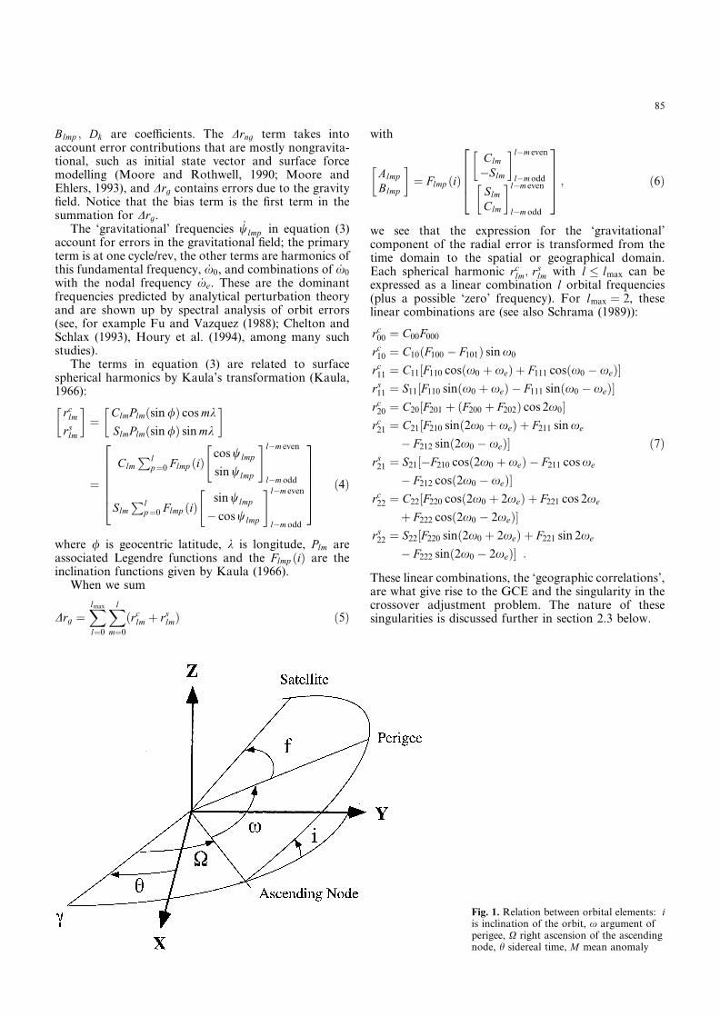
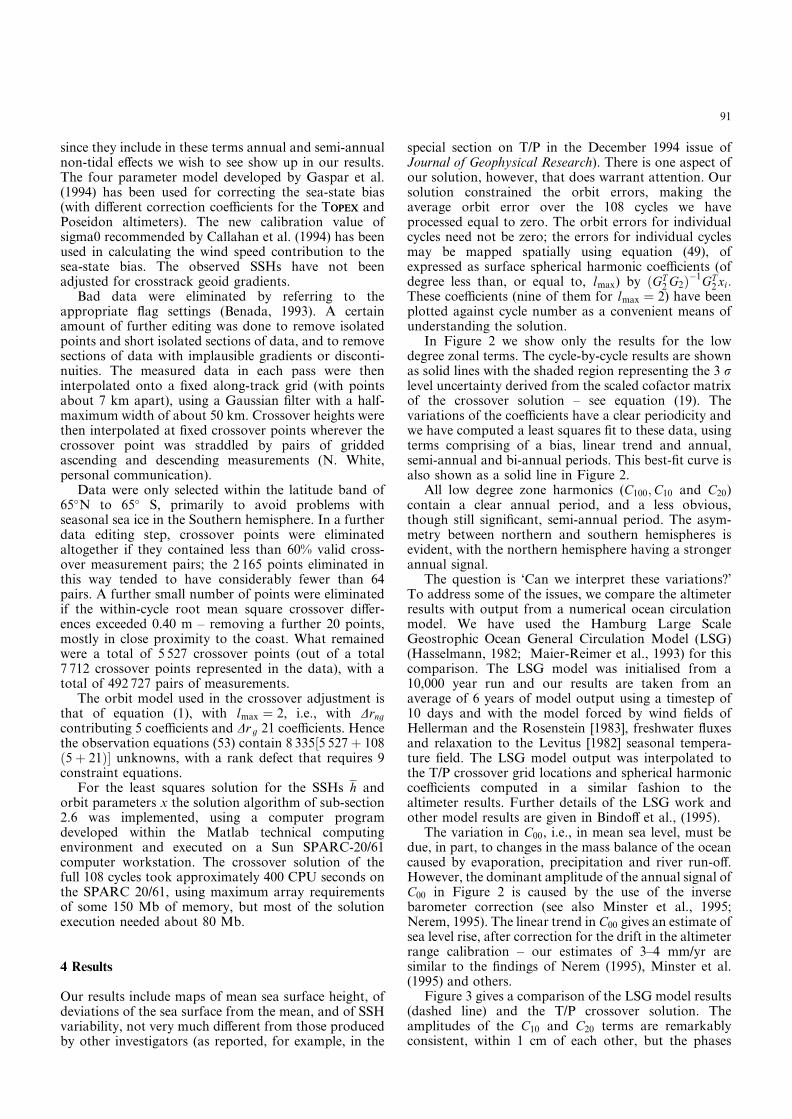
In Figure 2 we show only the results for the lowdegree zonal terms. The cycle-by-cycle results are shownas solid lines with the shaded region representing the 3 rlevel uncertainty derived from the scaled cofactor matrixof the crossover solution – see equation (19). Thevariations of the coefficients have a clear periodicity andwe have computed a least squares fit to these data, usingterms comprising of a bias, linear trend and annual,semi-annual and bi-annual periods. This best-fit curve isalso shown as a solid line in Figure 2.

All low degree zone harmonics (C100; C10 and C20)contain a clear annual period, and a less obvious,though still significant, semi-annual period. The asym-metry between northern and southern hemispheres isevident, with the northern hemisphere having a strongerannual signal.

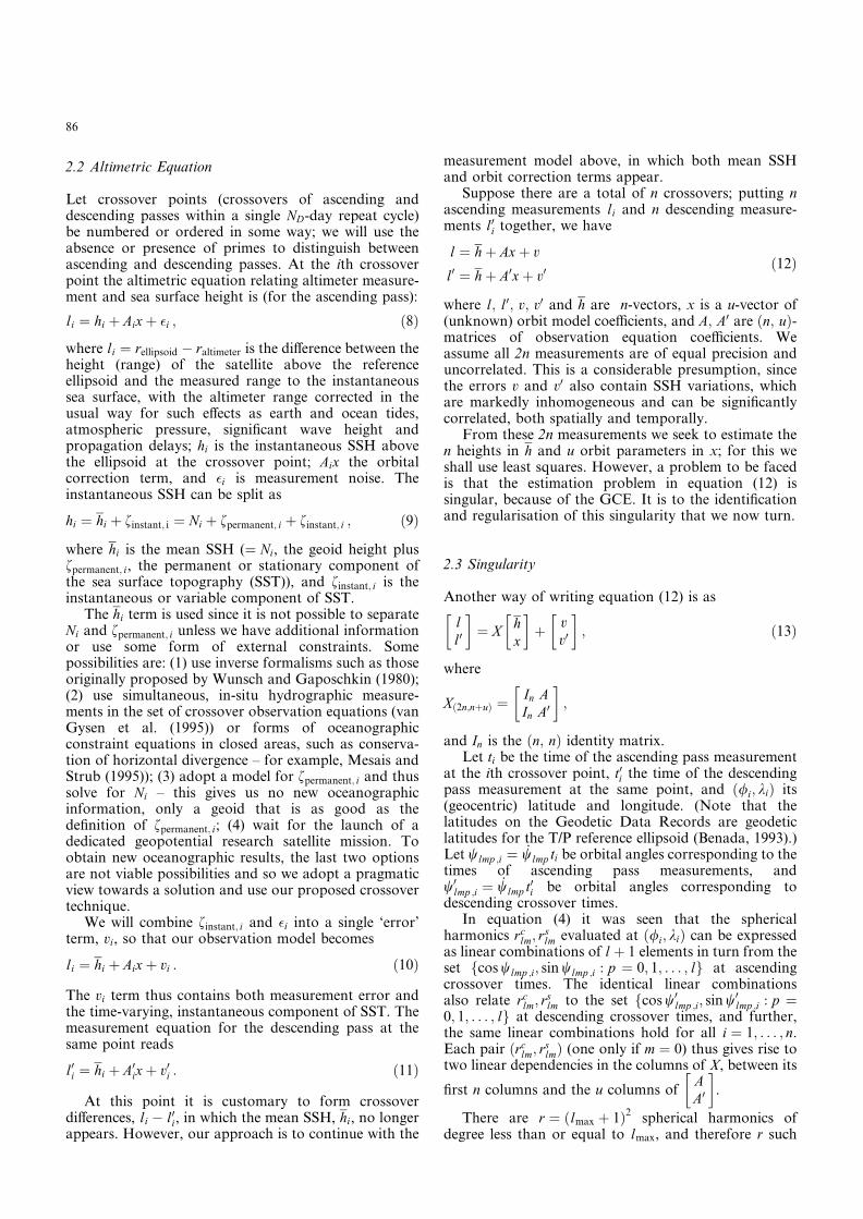
The question is ‘Can we interpret these variations?’To address some of the issues, we compare the altimeterresults with output from a numerical ocean circulationmodel. We have used the Hamburg Large ScaleGeostrophic Ocean General Circulation Model (LSG)(Hasselmann, 1982; Maier-Reimer et al., 1993) for thiscomparison. The LSG model was initialised from a10,000 year run and our results are taken from anaverage of 6 years of model output using a timestep of10 days and with the model forced by wind fields ofHellerman and the Rosenstein [1983], freshwater fluxesand relaxation to the Levitus [1982] seasonal tempera-ture field. The LSG model output was interpolated tothe T/P crossover grid locations and spherical harmoniccoefficients computed in a similar fashion to thealtimeter results. Further details of the LSG work andother model results are given in Bindoff et al., (1995).

The variation in C00, i.e., in mean sea level, must bedue, in part, to changes in the mass balance of the oceancaused by evaporation, precipitation and river run-off.However, the dominant amplitude of the annual signal ofC00 in Figure 2 is caused by the use of the inversebarometer correction (see also Minster et al., 1995;Nerem, 1995). The linear trend in C00 gives an estimate ofsea level rise, after correction for the drift in the altimeterrange calibration – our estimates of 3–4 mm/yr aresimilar to the findings of Nerem (1995), Minster et al.(1995) and others.

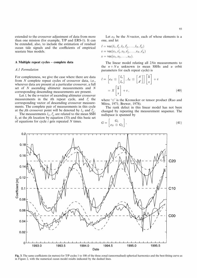
Figure 3 gives a comparison of the LSG model results(dashed line) and the T/P crossover solution. Theamplitudes of the C10 and C20 terms are remarkablyconsistent, within 1 cm of each other, but the phases

91

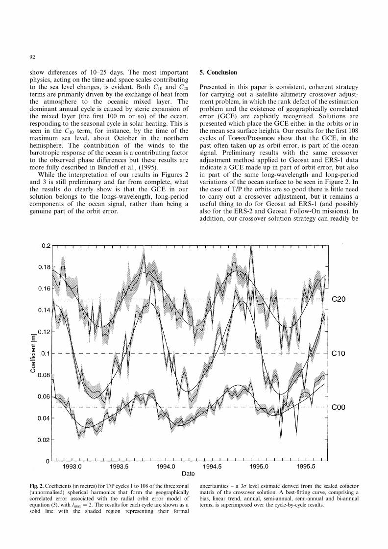
show differences of 10–25 days. The most importantphysics, acting on the time and space scales contributingto the sea level changes, is evident. Both C10 and C20terms are primarily driven by the exchange of heat fromthe atmosphere to the oceanic mixed layer. Thedominant annual cycle is caused by steric expansion ofthe mixed layer (the first 100 m or so) of the ocean,responding to the seasonal cycle in solar heating. This isseen in the C10 term, for instance, by the time of themaximum sea level, about October in the northernhemisphere. The contribution of the winds to thebarotropic response of the ocean is a contributing factorto the observed phase differences but these results aremore fully described in Bindoff et al., (1995).

While the interpretation of our results in Figures 2and 3 is still preliminary and far from complete, whatthe results do clearly show is that the GCE in oursolution belongs to the longs-wavelength, long-periodcomponents of the ocean signal, rather than being agenuine part of the orbit error.

5. Conclusion

Presented in this paper is consistent, coherent strategyfor carrying out a satellite altimetry crossover adjust-ment problem, in which the rank defect of the estimationproblem and the existence of geographically correlatederror (GCE) are explicitly recognised. Solutions arepresented which place the GCE either in the orbits or inthe mean sea surface heights. Our results for the first 108cycles of TOPEXOPEX/POSEIDONOSEIDON show that the GCE, in thepast often taken up as orbit error, is part of the oceansignal. Preliminary results with the same crossoveradjustment method applied to Geosat and ERS-1 dataindicate a GCE made up in part of orbit error, but alsoin part of the same long-wavelength and long-periodvariations of the ocean surface to be seen in Figure 2. Inthe case of T/P the orbits are so good there is little needto carry out a crossover adjustment, but it remains auseful thing to do for Geosat ad ERS-1 (and possiblyalso for the ERS-2 and Geosat Follow-On missions). Inaddition, our crossover solution strategy can readily be

Fig. 2. Coefficients (in metres) for T/P cycles 1 to 108 of the three zonal(unnormalised) spherical harmonics that form the geographicallycorrelated error associated with the radial orbit error model ofequation (3), with lmax � 2. The results for each cycle are shown as asolid line with the shaded region representing their formal

uncertainties – a 3r level estimate derived from the scaled cofactormatrix of the crossover solution. A best-fitting curve, comprising abias, linear trend, annual, semi-annual, semi-annual and bi-annualterms, is superimposed over the cycle-by-cycle results.

92

extended to the crossover adjustment of data from morethan one mission (for example, T/P and ERS-1). It canbe extended, also, to include the estimation of residualocean tide signals and the coefficients of empiricalseastate bias models.

A Multiple repeat cycles – complete data

A.1 Formulation

For completeness, we give the case where there are datafrom N complete repeat cycles of crossover data, i.e.,wherever data are present at a particular crossover, a fullset of N ascending altimeter measurements and Ncorresponding descending measurements are present.

Let li be the n-vector of ascending altimeter crossovermeasurements in the ith repeat cycle, and l0i thecorresponding vector of descending crossover measure-ments. The complete pair of measurements in this cycleat the jth crossover point will be denoted by lij and l0ij:

The measurements lij; l0ij are related to the mean SSHhj at the jth location by equation (33) and this basic setof equations for cycle i gets repeated N times.

Let eN be the N-vector, each of whose elements is aone, and let

l � vec�l1; l01; l2; l02; . . . ; lN ; l0N �

v � vec�v1; v01; v2; v02; . . . ; vN ; v0N �

x � vec�x1; x2; . . . ; xN �:

The linear model relating all 2Nn measurements tothe n � N u unknown (n mean SSHs and u orbitparameters for each repeat cycle) is

l � eN

In

In

� �

; IN

A

A0

� �� �h

x

" #

� v

� Xh

x

" #

� v ; �40�

where ‘’ is the Kronecker or tensor product (Rao andMitra, 1971; Brewer, 1978).

The rank defect in this linear model has not beenchanged by repeating the measurement sequence. Thenullspace is spanned by

G �

G1

eN G2

� �

; �41�

Fig. 3. The same coefficients (in metres) for T/P cycles 1 to 108 of the three zonal (unnormalised) spherical harmonics and the best-fitting curve asin Figure 2, with the numerical ocean model results indicated by the dashed lines.

93

and

XG � eN

In

In

� �

; IN

A

A0

� �� �G1

eN G2

� �

� eN

G1 � AG2

G1 � A0G2

� �

� 0�2Nn;r� ;

and rank(G) = rank�G1

eN G2

� �

� � r, as before.

The normal equations corresponding to equation (40)are

X T X hx

� �

� X T l ; �42�

where

X T X �

2NIn eTN �A � A0

�

eN �A � A0

�

T IN �AT A � A0T A0

�

� �

: �43�

A.2 Orbital constraints

We follow much the same procedure as in section 2.5.1above. The normal equation matrix X T X in equation(42) can be reduced to

2NIn eTN �A � A0

�

0 N22

� �

;

where

N22 � IN ÿ

1N

eN eTN

� �

�AT A � A0T A0

�

�

1N

eN eTN

12�A ÿ A0

�

T�A ÿ A0

� : �44�

The product of the two terms summed in this equation iszero, and �IN ÿ

1N eN eT

N �, being a projection matrix, is itsown pseudoinverse. In consequence, the pseudoinverseof N22 is the sum of the pseudoinverses of the two terms(Boullion and Odell, 1971):

N�

22 � �IN ÿ

1N

eN eTN � �AT A � A0T A0

�

ÿ1

�

1N

eN eTN Qx ; �45�

where Qx is given by equation (19).Hence

x � N�

22 IN ÿ

1N

eN eTN

A

A0

� �T (

�

1N

eN eTN

�

12

A ÿ A0

ÿ�A ÿ A0

�

� �T)

l

� IN ÿ

1N

eN eTN

� �

�AT A � A0T A0

�

ÿ1 A

A0

� �T

l

�

1N

eN eTN

12

QxA ÿ A0

ÿ�A ÿ A0

�

� �T

l �46�

or, breaking this up into solutions for individual cycles,

xi � y i ÿ1N

XN

j�1

yj �1N

XN

j�1

zj ; �47�

where

yj � �AT A � A0T A0

�

ÿ1�AT lj � A0T l0j�

zj �12Qx�A ÿ A0

�

T�lj ÿ l0j�

(cf. equation (20) for a single repeat cycle).The mean sea surface heights now follow by

substituting x into the first row of the normal equations(42):

h �

12N

eTN

In

In

� �T

l ÿ eTN �A � A0

�x

( )

;

but this result can be simplified by noting that

eTN �A � A0

�x � eTN

12�A � A0

�QxA ÿ A0

ÿ�A ÿ A0

�

� �T

l

� eTN �A � A0

�z;

where z � vec�z1; z2; . . . ; zN �: The solution for the meanSSHs thus becomes

h �

1N

XN

j�1

12flj � l0j ÿ �A � A0

�zg : �48�

Finally, it is easily verified that eTN GT

2 � x � 0, as werequire.

We thus see in equation (47) that the orbit errors xifor cycle i depend on data for all cycles, but that themean SSHs can be calculated as a simple mean ofaltimeter heights, corrected for orbit errors usingparameters zi calculated from a single cycle.

The constraint eTN GT

2 � x � 0 says that, on average,the orbit are free of GCE; nevertheless, for anyindividual cycle it need not follow that GT

2 xi � 0: Theamount by which the GCE within a cycle differs fromthe mean can be given its spatial expression by

Dhi � G1�GT2 G2�

ÿ1GT2 xi : �49�

A.3 SSH constraints

As before, we suggest that the easiest way to obtainmean SSHs and orbit parameters in which the GCE hasbeen placed in the orbits, and in which none of itappears in h; is through a transformation, as inequations (25) and (26).

For multiple repeat cycles the transformation fromthe orbit-constrained solution (or any other minimumconstraint solution) to the solution putting the con-straint into mean SSHs is

T � In�Nu ÿG1�GT

1 G1�ÿ1GT

1 0eN G2�GT

1 G1�ÿ1GT

1 0

" #

: �50�

94

In particular, the transformation for mean SSHs is

hSSH constrained � �In ÿ G1�GT1 G1�

ÿ1GT1 �horbit constrained;

�51�

a calculation which does not grow with the number ofrepeat cycles. Moreover, it is easy to see from equation(48) that conditions GT

1 hSSH constrained � 0 is satisfied.

A.4 Minimum norm solution

In a similar way the constrained orbit solution may alsobe transformed to a minimum norm solution, by thetransformation

X�

� TX g;

where X g is any minimum constraint solution (rightweak inverse), and where

T � In�Nu ÿ G�GT G�ÿ1GT�52�

with G, the matrix spanning the nullspace of X as givenin equation (38).

Again, it is easily verified that GT X�

� GT TX g� 0:

A.5 Residuals

The residuals, for multiple repeat cycles, are given bysomething akin to equation (31)

v � �In�Nu ÿ X X g�l : �53�

The residuals for cycle i can be calculated from

vi � li ÿ h ÿ Axi

v0i � l0i ÿ h ÿ A0xi

It bears repetition that the residuals do not depend onthe choice of right weak inverse X g

:

The residuals, as always, are orthogonal to the leastsquares solution space, i.e. orthogonal to the columnspace of X, i.e. X T v � 0: Now,

X T�

eTN �In; In�

IN �AT; A0T

�

� �

;

so the sum of the residuals at any crossover point is zero:

XN

i�1

�vij � v0ij� � 0 : �54�

Further, within each cycle

AT vi � A0T v0i � 0 :

In particular this means (since a bias is a part of the orbitmodel)

Xn

j�1

�vij � v0ij� � 0 ; �55�

i.e., all residuals within a cycle also sum to zero. Moregenerally, the residuals contain nothing (either spatiallyor temporally) that can be construed to be GCE.

Acknowledgement. We are grateful to Neil White, CSIRO Divisionof Oceanography, Hobart, Tasmania, for help with data prepara-tion. Nathan Bindoff and Jorg-Olaf Wolff provided the results fromthe ocean modelling comparisons. This work is supported by theAustralian Research Council (RC) and the University of NatalResearch Fund (HvG).

References

Benada, R., PO.DAAC Merged GDR (TOPEXOPEX/POSEIDONOSEIDON) UsersHandbook, JPL D-11007, Jet Propulsion Laboratory, Pasade-na, Calif., 1993.

Bertiger, W.I., Y.E. Bar-Sever, E.J. Christensen, E.S. Davis, J.R.Guinn, B.J. Haines, R.W. Ibanez-Meier, J.R. Jee, S.M. Lichten,W.G. Melbourne, R.J. Muellerschoen, T.N. Munson, Y. Vigue,S.C. Wu, T.P. Yunck, B.E. Schutz, P.A.M. Abusali, H.J. Rim,M.M. Watkins and P. Willis, GPS precise tracking of TOPEX/TOPEX/

POSEIDONPOSEIDON: Results and implications, J. Geophys. Res., 99,24449–24464, 1994.

Bindoff, N.L., R. Coleman, H. van Gysen and N.J. White,Comparison of seasonal sea-level signals from altimetry andocean models, paper presented at International Association ofthe Physical Sciences of the Ocean (IAPSO) XXI GeneralAssembly, Honolulu, Hawali, USA, August 5–12, 1995.

Blanc, F., P.Y. LeTraon and S. Houry, Reducing Orbit Error for aBetter Estimate of Oceanic Variability from Satellite Altimetry,J. Atmos. Oceanic Technol., 12, 150–160, 1995.

Brewer, J.W., Kronecker products and matrix calculus in systemtheory, IEEE Trans. Circ. Syst., CAS-25(9), 772–781, 1978.

Boullion, T.L., and P.L. Odell, Generalized Inverse Matrices,Wiley, New York, 1971.

Callahan, P.S., D.W. Hancock and G.S. Hayne, New sigma0calibration for the TOPEXTOPEX altimeter, TOPEX/Poseidon ResearchNews, 3, 28–30, 1994.

Chelton, D.B., and M.G. Schlax, Spectral characteristics of time-dependent orbit errors in altimeter height measurements, J.Geophys. Res., 98, 12579–12600, 1993.

Christensen, E.J., B.J. Haines, S.J. Keihm, C.S. Morris, R.S.Norman, G.H. Purcell, B.G. Williams, B.C. Wilson, G.H. Born,M.E. Parke, S.K. Gill, C.K. Shum, B.D. Tapley, R. Kolenkie-wicz and S. Nerem, Calibration of TOPEXOPEX/POSEIDONOSEIDON at PlatformHarvest, J. Geophys. Res., 99, 24465–24485, 1994.

Colombo, O.L., Altimetry, Orbits and Tides, NASA Tech. Memo.86180, NASA, Greenbelt MD, 1984.

Douglas, B.C., R.W. Agreen and D.T. Sandwell, Observing globalocean circulation with Seasat altimeter data, Mar. Geod., 8, 67–89, 1984.

Engelis, T., On the simultaneous improvement of a satellite orbitand determination of sea-surface topography using satellitealtimetry data, Manuscripta Geodaetica, 13, 180–190, 1988.

Fu, L.-L., and J. Vazquez, On correcting radial orbit errors foraltimetric satellites using crossover analysis, J. Atmos. OceanicTechnol., 5, 466–471, 1988.

Gaspar, P., F. Ogor, P.-Y. Le Traon and O.-Z. Zanife, Estimatingthe sea state bias of the TOPEXOPEX and POSEIDONOSEIDON altimeters fromcrossover differences, J. Geophys. Res., 99, 24981–24994, 1994.

Haines, B.J., G.H. Born, R.G. Williamson and C.J. Koblinsky,Application of the GEM-T2 gravity model to altimetric sateliteorbit computation, J. Geophys. Res., 99, 16237–16254, 1994.

Hasselmann, K., An ocean model for climate variability studies,Prog. Oceanography, 11, 69–92, 1982.

Heiskanen, W.A., and H. Moritz, Physical Geodesy, Freeman, SanFransisco, 1967.

95

Hellerman, S., and M. Rosenstein, Normal monthly wind stressover the world ocean with error estimates, J. Phys. Oceanogr,13, 1093–1104, 1983.

Houry, S., J.F. Minster, C. Broussier, K. Dominh, M.C. Gennero,A. Cazenave and P. Vincent, Radial orbit error reduction andmean sea surface computation from the Geosat altimeter data,J. Geophys. Res., 99, 4519–4531, 1994.

Kaula, W.M., Theory of Satellite Geodesy, Blaisdell, WalthamMass., 1966

Leick, A., GPS Satellite Surveying, Wiley, New York, 1990.Le Traon, P.Y., J. Stum, J. Dorandev, P. Gaspar and P. Vincent,

Global statistical analysis of TOPEXOPEX and POSEIDONOSEIDON data, J.Geophys. Res., 99, 24619–24631, 1994.

Levitus, S., Climatological Atlas of the World Ocean, NOAAProfessional Paper 13, U.S. Department of Commerce, 1982.

Maier-Reimer, E., U. Mikolajewicz and K. Hasselmann, Meancirculation of the HAMBURG LSG OGCM and its sensitivityto the thermohaline surface forcing, J. Phys. Oceanogr., 23,731–757, 1993.

Menard, Y., E. Jeansou and P. Vincent, Calibration of TOPEXOPEX/POSEIDONOSEIDON altimeter at Lampedusa, J. Geophys. Res., 99, 24487–24504, 1994.

Mesias, J.M., and P.T. Strub, An Inversion Method to DetermineOcean Surface Currents Using Irregularly Sampled SatelliteAltimetry Data, J. Atmos. Oceanic Technol., 12, 830–849, 1995.

Miller, L., R. Cheney and J. Lillibridge, Blending ERS-1 altimetryand tide gauge data, Eos Trans. AGU, 74, 185, 197, 1993.

Minster, J.-F., C. Brossier and P. Rogel, Variation of the mean sealevel from TOPEX/POSEIDON data, J. Geophys. Res., 100,(C12), 25,153–25,161, 1995.

Moore, P., and S. Ehlers, Orbital improvement of ERS-1 usingdual crossover arc techniques with TOPEXOPEX/POSEIDONOSEIDON, Manu-scripta Geodaetica, 18, 249–262, 1993.

Moore, P., and D.A. Rothwell, A study of gravitational and non-gravitational modelling errors in cross-over differences, Manu-scripta Goedaetica, 15, 187–206, 1990.

Nerem, R.S., Measuring global mean sea level variations usingTOPEX/POSEIDON altimeter data, J. Geophys. Res., 100,C12, 25,135–25,151, 1995.

Rao, C.R., and S.K. Mitra, Generalised Inverse of Matrices and itsApplications, Wiley New York, 1971.

Rapp, R.H., Geos-3 data processing for the recovery of geoidundulations and gravity anomalies, J. Geophys. Res., 84, 3784–3792, 1979.

Rapp, R.H., Y. Yi and Y.M. Wang, Mean sea surface and geoidgradient comparisons with TOPEXTOPEX altimeter data, J. Geophys.Res., 99, 24657–24667, 1994.

Ray, R.D., Atmospheric tides and the TOPEXOPEX/POSEIDONOSEIDON meteor-ological corrections, TOPEX/Poseidon Research News, 3, 12–14, 1994.

Rosborough, G.W., Satellite orbit perturbations due to thegeopotential, CSR-86-1, Center for Sapce Research, TheUniversity of Texas at Austin, 1986.

Schrama, E.J.O., The role of orbit errors in processing of satellitealtimeter data, Netherlands Geod. Commn., Delft, 1989.

Schrama, E.J.O., Some remarks on several definitions of geogra-phically correlated orbit errors: consequences for satellitealtimetry, Manuscripta Geodaetica, 17, 282–294, 1992.

Schrama, E.J.O., and R.D. Ray, A preliminary tidal analysis ofTOPEXOPEX/POSEIDONOSEIDON altimetry, J. Geophys. Res., 99, 24799–24808,1994.

Schum, C.K., D.N. Yuan, J.C. Ries, J.C. Smith, B.E. Schutz, andB.D. Tapley, Precision orbit determination for the Geosat ExactRepeat Mission, J. Geophys. Res., 95, 2887–2898, 1990.

Stammer, D., and C. Wunsch, Preliminary assessment of theaccuracy and precision of TOPEXOPEX/POSEIDONOSEIDON altimeter data withrespect to the large scale ocean circulation, J. Geophys. Res., 99,24584–245604, 1994.

Tai, C.-K., On Determining the Large-Scale Ocean CirculationFrom Satellite Altimetry, J. Geophys. Res., 88, 9553–9565,1983.

Tai, C.-K., Geosat crossover analysis in the Tropical Pacific 1.Constrained sinusoidal crossover adjustment, J. Geophys. Res.,93, 10621–10629, 1988.

Tai, C.-K., How to Observe the Gyre to Global-Scale Variability inSatellite Altimetry: Signal Attenuation by Orbit Error Removal,J. Atmos. Oceanic Technol., 8, 271–288, 1991.

Tai, C.-K., and L.-L. Fu, On crossover adjustment in satellitealtimetry and its oceanographic implications, J. Geophys. Res.,91, 2549–2554, 1986.

Tai, C.-K., and C.A. Wagner, Along-track spectra of oceanseasonal cycle and their attenuation by various orbit errorremoval schemes in satellite altimetry, U.S. Dept. of Commerce,NOAA Memo. OES-010, Washington D.C., 16pp, 1994.

Tapley, B.D., J.C. Ries, G.W. Davis, R.J. Eanes, B.E. Schutz, C.K.Shum, M.M. Watkins, J.A. Marshall, R.S. Nerem, B.H. Putney,S.M. Klosko, S.B. Luthcke, D. Pavlis, R.G. Williamson andN.P. Zelensky, Precision orbit determination for TOPEXOPEX/POSEIDONOSEIDON, J. Geophys. Res., 99, 24383–24404, 1994.

TOPEXOPEX/POSEIDONOSEIDON Project, GDR User’s Handbook, JPL D-8944, JetPropulsion Laboratory, Calif., 1992.

Van Gysen, H., R. Coleman and B. Hirsch, Local CrossoverAnalysis of Exactly Repeating Satellite Altimeter Data,submitted to Manuscripta Geodaetica, 1995.

Wagner, C.A., Radial variations of a satellite due to gravitationalerrors: implications for satellite altimetry, J. Geophys. Res., 90,3027–3036, 1985.

Wagner, C.A., and R.E. Cheney, Global sea level change fromsatellite altimetry, J. Geophys. Res., 97, 15607–15615, 1992.

Wagner, C.A., and C.K. Tai, Degradation of ocean signals insatellite altimetry due to orbit error removal processes, J.Geophys. Res., 99, 16255–16267, 1994.

Wang, Y.M., and R.H. Rapp, Geoid gradients for Geosat andTOPEXOPEX/POSEIDONOSEIDON repeat ground tracks, Department of GeodeticScience and Surveying, Ohio State University, Report No 408,1991.

White, N.J., R. Coleman, J.A. Church, P.J. Morgan and S.J.Walker, A southern hemisphere verification for the TOPEXOPEX/POSEIDONOSEIDON altimeter mission, J. Geophys. Res., 99, 24505–24516,1994.

Wunsch, C., and V. Zlotnicki, The accuracy of altimetric surfaces,Geophys.J.Roy.Astron.Soc., 78, 795–808, 1984.

Wunsch, C., and E.M. Gaposchkin, On using satellite altimetry todetermine the general circulation of the oceans with applicationto geoid improvement, Rev. Geophys. Space Phys., 18, 725–745,1980.

96