on the melan equation for suspension bridgesgazzola/melan.pdf2 the derivation of the melan equation...
TRANSCRIPT
On the Melan equation for suspension bridges
Filippo GAZZOLA
Dipartimento di Matematica del Politecnico, Piazza L. da Vinci 32 - 20133 Milano (Italy)
Mohamed JLELI - Bessem SAMET
Department of Mathematics, King Saud University, Riyadh (Saudi Arabia)
Dedicated to Andrzej Granas
Abstract
We first recall how the classical Melan equation for suspension bridges is derived. We discuss theorigin of its nonlinearity and the possible form of the nonlocal term: we show that some alternativeforms may lead to fairly different responses. Then we prove several existence results through fixed pointstheorems applied to suitable maps. The problem appears to be ill posed: we exhibit a counterexample touniqueness. Finally, we implement a numerical procedure in order to try to approximate the solution; itturns out that the fixed point may be quite unstable for actual suspension bridges. Several open problemsare suggested.
1 Introduction and historical overview
The celebrated report by Navier [19], published in 1823, was for several decades the only mathematicaltreatise of suspension bridges. It mainly deals with the static of cables and their interaction with towers:some second order ODE’s are derived and solved. At that time, no stiffening trusses had yet appeared andthe models suggested by Navier are oversimplified in several aspects. In spite of a lack of prior history, thereport by Navier appears as a masterpiece of amazing precision, including a part of applications intended tosuggest how to plan some suspension bridges, see [19, Troisieme Partie].
In the 19th century some further contributions deserve to be mentioned. The Theory of structures, containedin the monograph by Rankine [23], makes an analysis of the general principles governing chains, cords, ribsand arches; the part on suspension bridge with sloping rods [23, pp.171-173] makes questionable assumptionsand rough approximations. As far as we are aware, this contribution has not been applied to real bridges. In1875, Castigliano [5] suggested a new theory for elastic systems close to equilibrium and proved a resultknown nowadays as the Castigliano Theorem; this theorem became the core of his main work [6] publishedin 1879. His method allows to study the deflection of structures by strain energy method. His Theorem ofthe derivatives of internal work of deformation extended its application to the calculation of relative rotationsand displacements between points in the structure and to the study of beams in flexure.
A milestone theoretical contribution to suspension bridges is the monograph by the Czech engineer Melan[18], whose first edition goes back to 1888. This book was translated in English by Steinman who, in thepreface to his translation, writes The work has been enthusiastically received in Europe where it has alreadygone through three editions and the highest honors have been awarded the author. Melan considers thebridges with all those forms of construction having the characteristic of transmitting oblique forces to theabutments even when the applied loads are vertical in direction. Melan makes a detailed study of the staticof cables and beams through a careful analysis of the different kinds of suspension bridges according to the
1
number of spans, the stiffened or unstiffened structure, the effect of temperature. He repeatedly uses theCastigliano Theorem, in particular for the computation of deflection [18, p.69]. Melan [18, p.77] suggesteda fourth order equation to describe the behavior of suspension bridges; he views a suspension bridge as anelastic beam suspended to a sustaining cable (see Figure 1 below) and his equation reads
EI w′′′′(x)− (H + h(w)) w′′(x) +q
Hh(w) = p(x) ∀x ∈ (0, L) (1)
and is the object of the present paper. In Section 2 we derive (1) in full detail and we explain the physicalmeaning of all the terms. Biot-von Karman [3, (5.5)] call (1) the fundamental equation of the theory of thesuspension bridge.
It is our purpose to discuss the Melan equation (1) from several points of view. First of all, the term h(w)(representing the additional tension of the sustaining cable due to live loads) makes (1) a nonlinear nonlocalequation and, for this reason, it is often considered as a constant in the engineering literature. However, thenonlinear structural behavior of suspension bridges is by now well established, see e.g. [4, 11, 13, 15, 21].Therefore, the term h(w) deserves a special attention. In Section 3 we give a survey of the possible forms ofh usually considered in literature while in Section 4 we discuss the differences between these forms; it turnsout that there may be significant discrepancies.
In Section 5 we prove existence results for (1) by applying some fixed point theorems. A fairly wide classof nonlocal terms h(w) is considered. Since we were unable to prove general uniqueness results we soughta counterexample: we found a particular equation (1) admitting two solutions, a small one and a larger one.This raises some doubts about well-posedness of (1).
The Melan equation (1) has also attracted the interest of numerical analysts, see [9, 16, 24, 25, 29]. In thesepapers, several approximating procedures for the solution of (1) have been discussed for different forms of theterm h(w). In view of the above mentioned counterexample to uniqueness, one expects iterative numericalprocedures to be quite unstable. In Section 6 we suggest a unifying approach for equation (1) for a wide classof nonlocal terms h(w). We set up a fixed point iterative method which enables us to control the convergenceof the approximating terms h(wn), where {wn} is a sequence of possible approximations of the solutionof (1). Some numerical results testify that our approach may be used to get good approximate solutions,provided the parameters lie in some suitable range. In Section 7 we numerically study (1) with parameterstaken from an actual bridge, as suggested by Wollmann [29]: in this situation, fixed points appear to be quiteunstable and a different iterative procedure is used.
This paper is organized as follows. In Section 2 we derive the classical Melan equation. In Section 3 wediscuss three different approximations of the nonlocal term h(w) suggested in literature. In Section 4 wecompute the response of these approximations for some special forms of the beam. In Section 5 we state ourexistence results for the Melan equation (1), as well as a counterexample to uniqueness. In Sections 6 and 7we give some numerical results relative to our approximation scheme. Sections 8-10 are devoted to the proofsof the existence results. Finally, Section 11 contains our conclusions and some open problems.
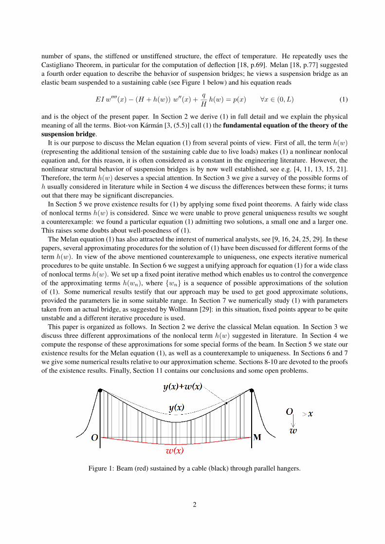
Figure 1: Beam (red) sustained by a cable (black) through parallel hangers.
2

2 The derivation of the Melan equation
The classical deflection theory of suspension bridges models the bridge structure as a combination of a string(the sustaining cable) and a beam (the roadway), see Figure 1. We follow here [3, VII.1]. The point O is theorigin of the orthogonal coordinate system and positive displacements are oriented downwards. The point Mhas coordinates M(0, L) where L is the distance between the two towers. When the system is only subject tothe action of dead loads, the cable is in position y(x) while the unloaded beam is the segment connecting Oand M . The cable is adjusted in such a way that it carries its own weight, the weight of the hangers and thedead weight of the roadway (beam) without producing a bending moment in the beam so that all additionaldeformations of the cable and the beam due to live loads are small. The cable is modeled as a perfectlyflexible string subject to vertical dead and live loads. When the string is subject to a downwards verticaldead load q(x) the horizontal component H > 0 of the tension remains constant. If the mass of the cable(dead load) is neglected then the load is distributed per horizontal unit. If we assume that spacing betweenhangers is small relative to the span, then the hangers can be considered as a continuous sheet or a membraneuniformly connecting the cable and the beam (live load). This is a simplified sketch of what occurs in asuspension bridge, provided that the mass of the cable is neglected and that the roadway is sought as a beam.The resulting equation reads (see [3, (1.3),VII]):
Hy′′(x) = −q(x) . (2)
If the endpoints of the string are at the same level γ (as in suspension bridges, see Figure 1) and if the deadload is constant, q(x) ≡ q, then the solution of (2) and the length Lc of the cable are given by
y(x)=γ+q
2Hx(L− x) , Lc=
∫ L
0
√1+y′(x)2 dx=
L
2
√1+
q2L2
4H2+H
qlog
(qL
2H+
√1+
q2L2
4H2
). (3)
Hence, the cable takes the shape of a parabola (y is positive downwards so that it has a ∪-shaped graph).Summarizing, we denote by
L the length of the beam at rest (the distance between towers) and x ∈ (0, L) the position on the beam;q and p = p(x) the dead and live loads per unit length applied to the beam;y = y(x) the downwards displacement of the cable connecting the endpoints (at level γ), due to the dead loadq;Lc the length of the cable subject to the dead load q;w = w(x) the downwards displacement of the beam and, hence, the additional displacement of the cable dueto the live load p;H the horizontal tension in the cable, when subject to the dead load q only;h = h(w) the additional tension in the cable produced by the live load p.
The function w describes both the downwards displacements of the beam and the cable because the elasticdeformation of the hangers is neglected. This classical assumption is justified by precise studies on linearizedmodels, see [17]. Since the dead load q of the beam is constant, (3) yields
y′′(x) = − q
H, y′(x) =
q
H
(L
2− x)
∀x ∈ (0, L) . (4)
When the live load p is added, a certain amount p1 of p is carried by the cable whereas the remaining partp − p1 is carried by the bending stiffness of the beam. In this case, it is well-known [3, 12, 18] that theequation for the (downwards) displacement w of the beam is
EI w′′′′(x) = p(x)− p1(x) ∀x ∈ (0, L) . (5)
The horizontal tension of the cable is increased toH+h(w) and the deflectionw is added to the displacementy. Hence, according to (2), the equation which takes into account this condition reads
(H + h(w))(y′′(x) + w′′(x)
)= −q − p1(x) ∀x ∈ (0, L) . (6)
3

Then, by combining (4)-(5)-(6) we obtain
EI w′′′′(x)− (H + h(w)) w′′(x) +q
Hh(w) = p(x) ∀x ∈ (0, L) , (7)
which is known in literature as the Melan equation [18, p.77]. The beam representing the bridge is assumedto be hinged at its endpoints, which means that the boundary conditions to be associated to (7) read
w(0) = w(L) = w′′(0) = w′′(L) = 0 . (8)
The equation (7) is by far nontrivial: it is a nonlinear integrodifferential equation of fourth order. A furthersimplification is to consider h as a small constant (see e.g. [7, (4.10)]) and obtain the linear equation
EI w′′′′(x)− (H + h)w′′(x) = p(x)− hq
H∀x ∈ (0, L)
which can be integrated with classical methods. In the engineering literature, (7) and its simplifications havebeen used for the computation of moments and shears for different kinds of suspension bridges, see [18, 26].
3 How to compute the additional tension
In this section we address the problem of the computation of the additional tension h = h(w) in (7). Sincethe cable is extensible, it may be that h(w) 6= 0. To fix the ideas, we first recall that the sag-span ratio isaround 1/10, see e.g. [22, Section 15.17]; by using both (3) and (4), this means that
y
(L
2
)− y(0) =
L
10=⇒ q
H=
4
5L=⇒ y′(0) = 0.4 . (9)
The length Lc of the cable at rest is given by
Lc =
∫ L
0
√1 + y′(x)2 dx =
L
2
√1 +
L2q2
4H2+H
qlog
(Lq
2H+
√1 +
L2q2
4H2
).
If we assume (9) then Lc may be written as a linear function of L:
Lc =
(√29
10+
5
4log
2 +√
29
5
)L ≈ 1.026L . (10)
The increase ∆Lc of the length Lc due to the deformation w is
∆Lc = Γ(w) :=
∫ L
0
(√1 + [y′(x) + w′(x)]2 −
√1 + y′(x)2
)dx . (11)
According to (4) and (11), the exact value of Γ(w) is
Γ(w) =
∫ L
0
√1 +
[w′(x) +
q
H
(L
2− x)]2
dx− Lc . (12)
Finally, if A denotes the cross-sectional area of the cable and E denotes the modulus of elasticity of thematerial, then the additional tension in the cable produced by the live load p is given by
h =EA
Lc∆Lc , h(w) =
EA
LcΓ(w) . (13)
In literature, there are at least three different ways to approximate Γ(w). Let us analyze them in detail.
4

First approximation. Recall the asymptotic expansion, valid for any ρ 6= 0,√1 + (ρ+ ε)2 −
√1 + ρ2 ∼ ερ√
1 + ρ2as ε→ 0 . (14)
By applying it to (12) one obtains
∆Lc ≈∫ L
0
y′(x)w′(x)√1 + y′(x)2
dx (15)
While introducing the model in Figure 1, Biot-von Karman [3, p.277] warn the reader by writing
whereas the deflection of the beam may be considered small, the deflection of the string, i.e., the deviationof its shape from a straight line, has to be considered as of finite magnitude.
However, after reaching (15), Biot-von Karman [3, (5.14)] decide to neglect y′(x)2 in comparison with unityand write
Γ(w) ≈ Γ1(w) =
∫ L
0y′(x)w′(x) dx = −
∫ L
0w(x)y′′(x) dx =
q
H
∫ L
0w(x) dx
where the integration by parts takes into account that w(0) = w(L) = 0 and, for the second equality, oneuses (4). We denote by Γ1 the approximated quantity obtained in [3]. A first approximation of Γ(w) is then
Γ1(w) =q
H
∫ L
0w(x) dx . (16)
Assuming that y′(x) is small means that the cable is almost horizontal, which seems quite far from the truth.This is a mistake while deriving (16): it was already present in the Report [2, VI-5] and also appears in morerecent literature, see [29, (17)] and [8, (1)].
In order to quantify the error of this approximation, we notice that (9) yields√
1 + y′(0)2 ≈ 1.077 yieldingan error of 7.7% if we approximate with unity. The same error occurs at the other endpoint (x = L). Using
again (9), a similar computation leads to√
1 + y′(L4 )2 ≈ 1.02 yielding an error of 2%, while it is clear thatthere is no error at all at the vertex of the parabola x = L/2. In some particular situations one may also havea sag-span ratio of 1/8, in which case y′(0) = 1/2 and
√1 + y′(0)2 ≈ 1.12, yielding an error of 12%. In
any case, this approximation appears too rude.
Second approximation. After reaching (11), Timoshenko [27] (see also [28, Chapter 11]) multiplies anddivides the integrand by its conjugate expression and obtains
Γ(w) =
∫ L
0
2w′(x)y′(x) + w′(x)2√1 + [y′(x) + w′(x)]2 +
√1 + y′(x)2
dx .
Then he neglects the derivatives and approximates the denominator with 2:
Γ(w) ≈∫ L
0
(w′(x)y′(x) +
w′(x)2
2
)dx .
With an integration by parts and taking into account both w(0) = w(L) = 0 and (4) we obtain
Γ2(w) =q
H
∫ L
0w(x) dx+
∫ L
0
w′(x)2
2dx . (17)
With two further integration by parts one may also obtain (see [28, (11.16)])
Γ2(w) =q
H
∫ L
0w(x) dx− 1
2
∫ L
0w(x)w′′(x) dx
5
but we prefer to stick to (17) since it does not involve the second derivative of w. Note that also Γ2 is obtainedby neglecting y′ which, as already underlined, is not small compared to unity, especially near the endpointsx = 0 and x = L.
Third approximation. Without neglecting y′, an integration by parts and the conditions w(0) = w(L) = 0transform (15) into
∆Lc ≈ −∫ L
0
y′′(x)w(x)
(1 + y′(x)2)3/2dx.
Hence, invoking (4), a third approximation of Γ is
Γ3(w) =q
H
∫ L
0
w(x)[1 + q2
H2
(x− L
2
)2]3/2dx . (18)
In order to obtain (18), one uses the asymptotic expansion (14) which holds for any ρ 6= 0 and for |ε| � |ρ|.But, in our case, from (4) we have that ρ = y′(x) and hence ρ = 0 if x = L
2 . More generally, since y is givenand w depends on the load p, |w′(x)| may not be small when compared to |y′(x)|. So, a second mistake isthat (14) is not correct for any x ∈ (0, L). Nevertheless, if the live load p = p(x) is assumed to be symmetricwith respect to x = L
2 (the center of the beam) also the displacement w will have such symmetry and then|w′(x)| will indeed be small with respect to |y′(x)| for all x; in particular, w′(L2 ) = y′(L2 ) = 0. Hence, thisapproximation appears reasonable only if the live load p is “almost” symmetric.
Note that Γ2 equals Γ1 plus an additional positive term and that Γ3 has a smaller integrand when comparedto Γ1; therefore,
Γ3(w) < Γ1(w) < Γ2(w) ∀w . (19)
In the next sections we compare (12)-(16)-(17)-(18) and we show that there may be large discrepancies.
4 Some explicit computations
In this section we estimate the difference of behaviors of Γi for some particular vertical displacements w. Tothis end, we notice that it is likely to expect that the maximum vertical displacement of the beam is around1/100 of the length of the span; if the bridge is 1 km long, the maximum amplitude of the vertical oscillationshould be expected of at most 10m. Whence, a reasonable assumption is that
w
(L
2
)=
L
100. (20)
We now compute the Γi’s on three different configurations of the beam.
Parabolic shape. Assume that the displacement w has the shape of a parabola,
w(x) = δx(L− x) (δ > 0), (21)
although this does not represent a hinged beam since it fails to satisfy the conditions w′′(0) = w′′(L) = 0.However, this simple case allows by hand computations and gives a qualitative idea of the differences betweenΓ and its approximations Γi (i = 1, 2, 3). For the configuration (21), the constraint (20) implies that
δ =1
25L. (22)
Let w be as in (21): then (12)-(16)-(17)-(18), combined with (9) and (22), yield
Γ(w) =
[√746− 5
√29
50+
25
22log
11 +√
746
25− 5
4log
2 +√
29
5
]L , Γ1(w) =
2
375L ,
6

Γ2(w) =7
1250L =
21
20Γ1(w) , Γ3(w) =
[√29
4− 25
16log
33 + 4√
29
25
]L
25.
Whence, if w is as in (21) and we assume both (9) and (22), then
Γ1(w) ≈ Γ(w) , Γ2(w) ≈ 1.05 Γ(w) , Γ3(w) ≈ 0.96 Γ(w) .
Simplest symmetric beam shape. The simplest shape for a hinged beam is the fourth order polynomial
w(x) = δx(x3 − 2Lx2 + L3) (δ > 0) ; (23)
this function will also serve to build Counterexample 1. In this case, if we assume again (20), we obtain
δ =4
125L3. (24)
By putting (9) and (24) into (12) and using w as in (23), a numerical computation with Mathematica gives
Γ(w) ≈ 0.00512L .
In turn, by replacing (23) into (16)-(17)-(18) and by using (9) and (24) we find
Γ1(w) =16
3125L , Γ2(w) =
2808
546875L , Γ3(w) =
[23
5
√29− 123
4log
33 + 4√
29
25
]L
160.
Therefore,Γ1(w) ≈ Γ2(w) ≈ Γ(w) ≈ 1.05 Γ3(w) .
Asymmetric beams. We assume here that there is some load concentrated on the interval (0, `) for some` ∈ (0, L2 ) (the case ` > L
2 being specular) and that the corresponding deformation w has the shape of thepiecewise affine function
w(x) = σx if x ∈ (0, `) , w(x) =σ`
L− `(L− x) if x ∈ (`, L) (25)
so that w(`) = σ`. A reasonable value of σ satisfies the rule in (20), that is,
σ` = w(`) =`
50=⇒ σ =
1
50. (26)
By putting (25) into (12) and using both (9) and (26) (Γ is not linear with respect to σ) we find the formula
Γ(w) =
[Φ
(4 `
5L− 21
50
)−Φ
(−21
50
)+ Φ
(2
5+
1
50
`
L−`
)−Φ
(4 `
5L− 2
5+
1
50
`
L−`
)− 2Φ
(2
5
)]5
8L
where we also used (10) and Φ(s) = s√
1 + s2 + log(s+√
1 + s2). Some tedious computations show that
Γ(w)→[
21√
2941−√
2501
1250− 4√
29
25+ 2 log
(√
2501− 1)(√
2941 + 21)
1250(2 +√
29)
]5
8L as `→ L
2
Γ(w) ∼√
2941− 10√
29
50` as `→ 0 .
By putting (25) into (16)-(17)-(18) and using (9) we find
Γ1(w) =2`
5σ , Γ2(w) =
2`
5σ +
L `
L−`σ2
2, Γ3(w) =
(√29
4L−
√29
16L2+`2−L`
)σ L
L−`.
7

Both Γ1 and Γ3 linearly depend on σ. Summarizing, in the asymmetric case we find that
Γ1(w)
Γ(w)→ 1.054 ,
Γ2(w)
Γ(w)→ 1.08 ,
Γ3(w)
Γ(w)→ 1.015 as `→ 0 ,
yielding approximate errors of 5.4%, 8%, 1.5% respectively. Moreover,
Γ(w)
Γ1(w)→ 1.008 ,
Γ(w)
Γ2(w)→ 0.96 ,
Γ(w)
Γ3(w)→ 1.047 as `→ L
2,
yielding approximate errors of 0.8%, 4%, 4.7% respectively.
5 Existence and uniqueness results
Here and in the sequel we denote the Lp-norms by
‖v‖p := ‖v‖Lp(0,L) ∀p ∈ [1,∞] , ∀v ∈ Lp(0, L) .
In this section we prove the existence of at least a solution of (7)-(8). For simplicity, we drop some constantsand consider the problem
w′′′′(x)−(a+h(w)) w′′(x)+b h(w)=p(x) for x ∈ (0, L) , w(0)=w(L)=w′′(0)=w′′(L)=0 (27)
where a, b > 0 and h(w) is a nonlocal term, of indefinite sign, satisfying
∃c > 0 , |h(u)| ≤ c‖u‖1 ∀u ∈ H10 (0, L) . (28)
Note that assumption (28) is satisfied when h is defined by
h(w) =EA
LcΓi(w) (i = 1, 3) ,
see (13), with Γ1 and Γ3 defined in (16) and (18). In both these cases, one can take c = EALc
qH .
Our first results yields the existence of a solution of (27) provided that L and p are sufficiently small.
Theorem 1. Let a, b > 0 and let h : H10 (0, L) → R be a continuous functional such that there exists c > 0
satisfying (28). Assume that
L5 <π3
bc. (29)
Then for all p ∈ L1(0, L) satisfying
‖p‖1 ≤a(π3 − bc L5)
cL4(30)
there exists at least one solution w ∈W 4,1(0, L) ∩H10 (0, L) of (27) which satisfies the estimate
‖w‖∞ ≤L3
π3 − bc L5‖p‖1 .
We prove Theorem 1 in Section 8. Theorem 1 does not apply to Γ since the corresponding function h in(13) fails to satisfy (28). So, we now state a different result which allows to include Γ.
Consider again (27) with a, b > 0 and h(w) being a nonlocal term, of indefinite sign, satisfying
∃c > 0 , |h(u)| ≤ c‖u′‖1 ∀u ∈ H10 (0, L) . (31)
8

Note that assumption (31) is satisfied when h is defined by
h(w) =EA
LcΓ(w) ,
see (13), with Γ defined in (12). Indeed, from the simple inequality√1 + (γ + s)2 −
√1 + γ2 ≤ |s| ∀γ ∈ R , ∀s ∈ R ,
we infer that
|Γ(w)| ≤∫ L
0
∣∣∣√1 + [y′(x) + w′(x)]2 −√
1 + y′(x)2∣∣∣ dx ≤ ∫ L
0|w′(x)| dx
and therefore one can take c = 1 in (31). In Section 9 we prove
Theorem 2. Let a, b > 0 and let h : H10 (0, L) → R be a continuous functional such that there exists c > 0
satisfying (31). Assume that
L4 <1
bc. (32)
Then for all p ∈ L1(0, L) satisfying
‖p‖1 ≤a(1− bc L4)
cL3(33)
there exists at least one solution w ∈W 4,1(0, L) ∩H10 (0, L) of (27) which satisfies the estimate
‖w′‖∞ ≤L2
1− bc L4‖p‖1 .
Remark 3. Neither Theorem 1 nor Theorem 2 cover the case where h is defined through Γ2 since
|Γ2(w)| ≤ c‖w‖1 +‖w′‖22
2∀w ∈ H1
0 (0, L)
and therefore Γ2 has quadratic growth. However, using some a priori bounds for the linearized equation, onemay estimate the quadratic term ‖w′‖22 with a linear term ‖w′‖2 and, consequently, obtain a result in the spiritof Theorems 1 and 2 also when h is defined through Γ2. However, we will not pursue this here.
So far, we merely stated existence results for small solutions of (27). We now prove an existence anduniqueness result (for small solutions) which, however, has the disadvantage of some tedious and painfulassumptions. We first assume that
h(0) = 0 , ∃c > 0 , |h(u)− h(v)| ≤ c‖u′′ − v′′‖2 ∀u, v ∈ H2(0, L) ∩H10 (0, L) . (34)
When h is defined by (13), the condition (34) is satisfied for Γ, Γ1 or Γ3.In Section 10 we prove the following existence and uniqueness result for small solutions of (27) which,
again, holds when both L and p are sufficiently small.
Theorem 4. Let a, b > 0 and let h : H10 (0, L) → R be a continuous functional such that there exists c > 0
satisfying (34). Assume that
L < min
{1
(bc)2,
π
(bc)2/5
}. (35)
Then for all p ∈ L1(0, L) satisfying
‖p‖1 < min
{(πL
)3/2 (π5/2 − bc L5/2)(1− bc√L)
c(π5/2 − bc L5/2 + bcπ L7/2),a(π5/2 − bc L5/2)
πcL5/2
}(36)
there exists a unique solution w ∈W 4,1(0, L) ∩H10 (0, L) of (27) satisfying
‖w′′‖2 ≤π L5/2
π5/2 − bc L5/2‖p‖1 . (37)
9

Note that the smallness of L assumed in (35) ensures that the right hand side of (36) is positive. Clearly,which is the maximum to be considered in (35) depends on whether bc ≶ 1. We also emphasize that Theorem4 only states the existence and uniqueness of a small solution satisfying (37) but it does not clarify if thereexist additional large solutions violating (37). And, indeed, as the following counterexample shows, theremay exist additional large solutions and, hence, Theorem 4 cannot be improved without further assumptions.
Counterexample 1. For a given L >√
12 consider the functional
h(w) =
∫ L
0w′′(x) dx ∀w ∈ H2(0, L) ∩H1
0 (0, L)
so that (34) is satisfied with c =√L. Fix δ > 0, for instance as in (24), and consider the problem
w′′′′(x)−(2δL3+ε+h(w)
)w′′(x)+
12
L3h(w)=pε(x) for x ∈ (0, L) , w(0)=w(L)=w′′(0)=w′′(L)=0
(38)where pε(x) = 12δε(Lx− x2) and ε > 0 will be fixed later. The equation (38) is as (27) with
a = 2δ L3 + ε , b =12
L3, c =
√L , p(x) = pε(x) .
Whence,1
(bc)2=
L5
144,
π
(bc)2/5=
π L
122/5.
Since we assumed L >√
12 and since 122/5 < π, the condition (35) is satisfied. Now we choose ε > 0sufficiently small so that pε satisfies the bound (36). Then all the assumptions of Theorem 4 are fulfilled andthere exists a unique solution w of (38) satisfying (37).
Note that the function wδ(x) = δx(x3 − 2Lx2 + L3), already considered in (23), solves (38). However, ifε > 0 is sufficiently small, it fails to satisfy (37) and therefore wδ is not the small solution found in Theorem4. This shows that, besides a small solution, also a large solution may exist. 2
We conclude this section with a simple calculus statement which will be repeatedly used in the sequel,both for proving the above statements through a fixed point argument and for implementing the numericalprocedures.
Proposition 5. Let α > 0 and f ∈ L1(0, L). The unique solution u ∈W 4,1(0, L)∩H10 (0, L) of the problem
u′′′′(x)− α2 u′′(x) = f(x) in (0, L) , u(0) = u(L) = u′′(0) = u′′(L) = 0 (39)
is given by
u(x) =x
α2 L
∫ L
0(L− t)f(t) dt− sinh(αx)
α3 sinh(αL)
∫ L
0sinh[α(L− t)] f(t) dt
+
∫ x
0
[t− xα2
+sinh[α(x− t)]
α3
]f(t) dt .
Note that the assumption α2 > 0 in Proposition 5 is crucial since otherwise the equation changes type:instead of hyperbolic functions one has trigonometric functions with possible resonance problems.
10

6 Numerical implementations with a stable fixed point
In this section and the following one we apply an iterative procedure in order to numerically determine asolution of (27). We inductively construct sequences {wn} of approximating solutions and it turns out thatan excellent estimator of the rate of approximation is the corresponding numerical sequence {h(wn)}. As weshall see, depending on the parameters involved, the fixed points of our iterative methods may be both stableor unstable. In this section we deal with stable cases whereas in Section 7, which involves an actual bridge,we deal with an unstable case.
We drop here the constant EA/Lc so that h(w) = Γ(w), we fix constants a, b, c > 0 and a load p, andconsider the equations
aw′′′′(x)− (b+ h(w)) w′′(x) + c h(w) = p(x) ∀x ∈ (0, L) , (40)
complemented with the boundary conditions (8). We define a map Λ : R→ R as follows. For any Θ ∈ R wedenote by WΘ the unique solution of the equation
aw′′′′(x)− (b+ Θ) w′′(x) + cΘ = p(x) ∀x ∈ (0, L) ,
satisfying (8). The solution of this equation may be obtained by using Proposition 5. Then we put
Λ(Θ) := h(WΘ) . (41)
Clearly, WΘ is a solution of (40)-(8) if and only if Θ is a fixed point for Λ, that is, h(WΘ) = Λ(Θ) = Θ.If Λ(Θ) 6= Θ we can hope to find the fixed point for Λ by an iterative procedure. We fix some Θ0 ∈ R (for
instance, Θ0 = 0) and define a sequence Θn := Λ(Θn−1) for all n ≥ 1. This defines a discrete dynamicalsystem which, under suitable conditions, may force the sequence to converge to the fixed point Θ of Λ. Forthe equations considered in this section, this procedure works out perfectly.
In the tables below we report some of our numerical results; we always started with Θ0 = 0. For each tablewe emphasize the values of the parameters involved in (40). Since Θ turned out to be small, we magnifyΛ(Θn) by some powers of 10.
n 1 2 3 4 5 6 7 8
100 Λ(Θn) 9.55239 8.1815 8.37021 8.34408 8.3477 8.3472 8.34727 8.34726
Case L = 2, a = b = c = 1, p(x) ≡ 1.
n 1 2 3 4 5 6 7 8
10 Λ(Θn) 8.04928 4.80539 5.90186 5.50443 5.6451 5.59488 5.61276 5.60638
Case L = 2, a = b = c = 1, p(x) = 0 in (0, 1) and p(x) = 10 in (1, 2).
n 1 2 3 4 5 6 7 8
10 Λ(Θn) 3.93699 2.84652 3.1149 3.04668 3.06388 3.05954 3.06064 3.06036
Case L = 2, a = b = c = 1, p(x) = 0 in (0, 3/2) and p(x) = 20 in (3/2, 2).
11

n 1 2 3 4 5 6 7 8
10 Λ(Θn) 6.19365 3.96853 4.65526 4.4316 4.50324 4.48017 4.48758 4.4852
Case L = 2, a = b = c = 1, p(x) = 10e−10(x−1)2 .
n 1 2 3 4
100 Λ(Θn) 1.02565 1.01427 1.01439 1.01439
Case L = 2, a = 10, b = c = 1, p(x) ≡ 1.
n 1 2 3 4 5 6 7 8
100 Λ(Θn) 9.55239 0.3214 9.16847 0.60499 8.83393 0.858085 8.5387 1.08607
Case L = 2, a = b = 1, c = 10, p(x) ≡ 1.
In all the above results it appears that the sequence {Λ(Θn)} is not monotonic but the two subsequences ofodd and even iterations appear, respectively, decreasing and increasing. Moreover, since they converge to thesame limit, this means that
Λ(Θ2k) < Λ(Θ2k+2) < Θ < Λ(Θ2k+1) < Λ(Θ2k−1) ∀k ≥ 1 . (42)
This readily gives an approximation of Θ and, in turn, of the solution w of (40). As should be expected, theconvergence is slower for larger values of c: in the very last experiment we found 100 Λ(Θ126) < 4.3 and100 Λ(Θ127) > 4.7.
In all these cases this procedure worked out, which means that the fixed point Θ is stable and that thediscrete dynamical system may be described as in Figure 2. The map Θ 7→ Λ(Θ) is decreasing and its slopeis larger than −1 in a neighborhood of Θ.
Figure 2: The stable fixed point for the map Θ 7→ Λ(Θ) defined by (41).
We also used this iterative procedure in order to estimate the responses of the different forms of h = Γi. Wefix the parameters involved in (40) and we perform the iterative procedure for each one of the Γi (i = 1, 2, 3)and Γ0 = Γ. We define again Λi(Θ) (i = 0, 1, 2, 3) as in (41). After a finite number of iterations we have agood approximation of
Θi := limn→∞
Λi(Θn) .
12

Then, we obtain a limit equation (40) having the form
aw′′′′(x)−(b+ Θi
)w′′(x) + cΘi = p(x) ∀x ∈ (0, L) , (i = 0, 1, 2, 3) .
By integrating these linear equations with the boundary conditions (8) we obtain the different solutions. Inthe next two tables we quote our numerical results for the different values of Θi.
100 Θ0 100 Θ1 100 Θ2 100 Θ3
2.15633 2.07143 2.26845 1.98463
Case L = 2, a = c = 1, b = 10, p(x) ≡ 1.
100 Θ0 100 Θ1 100 Θ2 100 Θ3
7.7621 6.19506 8.47472 5.91363
Case L = 2, a = c = 1, b = 10, p(x) = 0 in (0, 3/2) and p(x) = 20 in (3/2, 2).
In all these experiments we found the same qualitative behavior represented in Figure 2: the sequence{Λi(Θn)} is not monotonic, it satisfies (42), and it converges to a fixed point for Λi. As we shall see in nextsection, this is not the case for different values of the parameters.
7 Numerics with an unstable fixed point for an actual bridge
We consider here a possible actual bridge and we fix the parameters in (7) following Wollmann [29]. Thestiffness EI is known to beEI = 57 ·106 kN ·m2 whereas EA = 36 ·108 kN . Wollmann considers a bridgewith main span of length L = 460m and he assumes (9) so that
q
H= 1.739 · 10−3m−1 , q = 170 kN/m , H = 97.75 · 103 kN .
By (10) we find Lc = 472m, while from (13) we infer
h(w) = (7.627 · 106 kN/m) Γi(w)
where the Γi(w) are measured in meters; we will consider i = 0, 1, 2, 3 with Γ0 = Γ as in (12) and theremaining Γi as in (16)-(17)-(18).
We first take as live load a vehicle, a coach of length 10m having a weight density of 10 kN/m, that is
p(x) = 10χ(d,d+10) kN/m 0 < d < 230 ,
where χ(d,d+10) denotes the characteristic function of the interval (d, d+ 10). Then, after dropping the unitymeasure kN/m and dividing by 10, (7) reads
57 · 105w′′′′(x)−(
9775 + 7.627 · 105 Γi(w))w′′(x) + 1326 Γi(w) = χ(d,d+10) ∀x ∈ (0, 460) (43)
where the solution w is computed in meters. For numerical reasons, it is better to rescale (43): we put
w(x) = v( x
230
)= v(s) . (44)
13

Let us compute the different values of Γi after this change. We have
Γ0(w) =
∫ 460
0
√1 + [w′(x) + 1.739 · 10−3 (230− x)]2 dx− 1.026 · 460
= 230
[∫ 2
0
√1 + [4.35 · 10−3 v′(s) + 0.4 (1− s)]2 ds− 2.052
]=: Υ0(v) ;
Γ1(w) = 1.739 · 10−3
∫ 460
0w(x) dx = 0.4
∫ 2
0v(s) ds =: Υ1(v) ;
Γ2(w) = 0.4
∫ 2
0v(s) ds+ 2.17 · 10−3
∫ 2
0v′(s)2 ds =: Υ2(v) ;
Γ3(w) = 1.739 · 10−3
∫ 460
0
w(x) dx
[1 + 3.02 · 10−6 (x− 230)2]3/2= 0.4
∫ 2
0
v(s) ds
[1 + 0.16(s− 1)2]3/2=: Υ3(v) .
Then, after the change (44) and division by 57·105
2304≈ 2.037 · 10−3, the equation (43) becomes
v′′′′(s)−(
90.72 + 7078 Υi(v))v′′(s) + 650999 Υi(v) = 491ψd(s) ∀s ∈ (0, 2) (45)
where ψd is the characteristic function of the interval ( d230 ,
d+10230 ). We try to proceed as in Section 6. We fix
some Θ > 0 and we solve the equation (45) by replacing Υi(v) with Θ:
v′′′′(s)− α2 v′′(s) = f(s) ∀s ∈ (0, 2) (46)
whereα2 := 90.72 + 7078 Θ , f(s) := 491ψd(s)− 650999 Θ .
By Proposition 5, this linear equation, complemented with hinged boundary conditions, admits a uniquesolution VΘ given by
VΘ(s) =
(491(455− d)
10580− 650999Θ
)s
α2+
650999Θ
2α2s2 +
650999Θ
α4
(1− cosh(α s)
)+
[650999Θ
(cosh(2α)− 1
)− 982 sinh
α
46sinh
α(455− d)
230
]sinh(α s)
α4 sinh(2α)+ 491 Ψd,Θ(s)
where
Ψd,Θ(s) =
0 if 0 ≤ s ≤ d
230
1α4
(cosh[α(s− d
230)]− 1)− (s− d
230)2
2α2 if d230 < s < d+10
230
2α4 sinh α
46 sinh(α(s− d+5
230
))+ 1
46α2
(d+5115 − 2s
)if d+10
230 ≤ s ≤ 2
.
We then compute Υi(VΘ) according to the above formulas and we put
Λi(Θ) = Υi(VΘ) . (47)
Again, this defines a sequence Θn = Λi(Θn−1). However, for the values in (45), this sequence appears todiverge and to be quite unstable: contrary to the experiments in Section 6, see (42), we have here that
Λi(Θ2k)→ +∞ , Λi(Θ2k+1)→ −∞ as k →∞ .
This clearly describes an unstable fixed point, as represented in Figure 3. Here, the slope of Θ 7→ Λi(Θ) issmaller than −1. In fact, our experiments show that it is very negative, possibly −∞.
14

Figure 3: The unstable fixed point for the map Θ 7→ Λi(Θ) defined by (47).
As already mentioned, in order to apply Proposition 5 one needs 90.72 + 7078 Θn > 0 since otherwisethe equation changes type. These difficulties suggest to proceed differently. We fix Θ0 = 0 and, for anyk ≥ 0, if Θ2k+1 = Λi(Θ2k) > Θ2k (resp. Θ2k+1 < Θ2k) we take some Θ2k+2 ∈ (Θ2k,Θ2k+1) (resp.Θ2k+2 ∈ (Θ2k+1,Θ2k)). With this procedure we constructed a new sequence such that (Θ2k+1 −Θ2k)→ 0as k →∞, that is,
∃ Θi = limn→∞
Θn (i = 0, 1, 2, 3) (48)
where the index i identifies which of the Υi’s is used to construct the sequence, see (47).We numerically computed these limits for different values of d, see the next table where we only report the
first digits of Θi: the results turned out to be very sensitive to modifications of these values up to 4 more digitsand our numerical procedure stopped precisely when Θ2k and Θ2k+1 had the first 7 nonzero digits coinciding.
d 0 50 100 225
Θ0 1.131 · 10−6 1.021 · 10−5 1.74 · 10−5 2.509 · 10−5
Θ1 9.842 · 10−7 1.016 · 10−5 1.729 · 10−5 2.477 · 10−5
Θ2 9.843 · 10−7 1.017 · 10−5 1.73 · 10−5 2.477 · 10−5
Θ3 9.672 · 10−7 1.005 · 10−5 1.723 · 10−5 2.492 · 10−5
Approximate value of the optimal constants Θi in (48), case of a single coach.
It appears that the best approximation of Θ0 is Θ2 if d = 0, 50, 100 (asymmetric load) whereas it is Θ3 ifd = 225 (almost symmetric load). The most frequently used approximation Θ1 is never the best one.
The corresponding solutions of (45), which we denote by vi, satisfy the linear equation
v′′′′i (s)−(
90.72 + 7078 Θi
)v′′i (s) + 650999 Θi = 491ψd(s) ∀s ∈ (0, 2)
and can be explicitly computed by means of Proposition 5. Instead of giving the analytic form, we plot thedifferences between these solutions. Since Θ1 ≈ Θ2 in all the above experiments, we also found that v1 ≈ v2.Therefore, in Figure 4 we only plot the functions v2 − v0 and v3 − v0.
We now take as live load a freight train of length 230m having a weight density of 20 kN/m, that is
p(x) = 20χ(d,d+230) kN/m 0 < d < 230
where χ(d,d+230) is the characteristic function of the interval (d, d+ 230). We consider both the cases wherethe train occupies the first half of the span (d = 0) and the case where the train is in the middle of the span
15
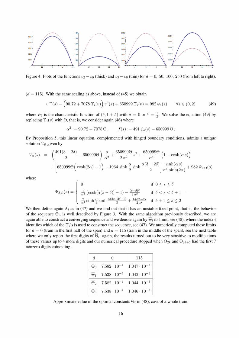
Figure 4: Plots of the functions v2− v0 (thick) and v3− v0 (thin) for d = 0, 50, 100, 250 (from left to right).
(d = 115). With the same scaling as above, instead of (45) we obtain
v′′′′(s)−(
90.72 + 7078 Υi(v))v′′(s) + 650999 Υi(v) = 982ψδ(s) ∀s ∈ (0, 2) (49)
where ψδ is the characteristic function of (δ, 1 + δ) with δ = 0 or δ = 12 . We solve the equation (49) by
replacing Υi(v) with Θ, that is, we consider again (46) where
α2 := 90.72 + 7078 Θ , f(s) := 491ψδ(s)− 650999 Θ .
By Proposition 5, this linear equation, complemented with hinged boundary conditions, admits a uniquesolution VΘ given by
VΘ(s) =
(491(3− 2δ)
2− 650999Θ
)s
α2+
650999Θ
2α2s2 +
650999Θ
α4
(1− cosh(α s)
)+
[650999Θ
(cosh(2α)− 1
)− 1964 sinh
α
2sinh
α(3− 2δ)
2
]sinh(α s)
α4 sinh(2α)+ 982 Ψδ,Θ(s)
where
Ψδ,Θ(s) =
0 if 0 ≤ s ≤ δ1α4 (cosh[α(s− δ)]− 1)− (s−δ)2
2α2 if δ < s < δ + 1
2α4 sinh α
2 sinh α(2s−2δ−1)2 + 1+2δ−2s
2α2 if δ + 1 ≤ s ≤ 2
.
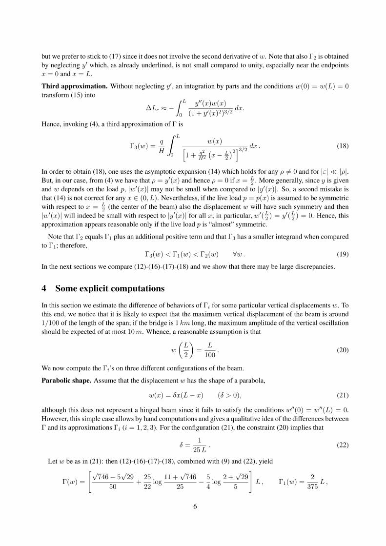
We then define again Λi as in (47) and we find out that it has an unstable fixed point, that is, the behaviorof the sequence Θn is well described by Figure 3. With the same algorithm previously described, we areagain able to construct a converging sequence and we denote again by Θi its limit, see (48), where the index iidentifies which of the Υi’s is used to construct the sequence, see (47). We numerically computed these limitsfor d = 0 (train in the first half of the span) and d = 115 (train in the middle of the span), see the next tablewhere we only report the first digits of Θi: again, the results turned out to be very sensitive to modificationsof these values up to 4 more digits and our numerical procedure stopped when Θ2k and Θ2k+1 had the first 7nonzero digits coinciding.
d 0 115
Θ0 7.582 · 10−4 1.047 · 10−3
Θ1 7.538 · 10−4 1.042 · 10−3
Θ2 7.582 · 10−4 1.044 · 10−3
Θ3 7.538 · 10−4 1.046 · 10−3
Approximate value of the optimal constants Θi in (48), case of a whole train.
16

Again, the best approximation of Θ0 is Θ2 if d = 0 (asymmetric load) whereas it is Θ3 if d = 115(symmetric load). And, again, Θ1 is never the best one.
The corresponding solutions of (49), which we denote by vi, satisfy the linear equation
v′′′′i (s)−(
90.72 + 7078 Θi
)v′′i (s) + 650999 Θi = 982ψδ(s) ∀s ∈ (0, 2)
and can be explicitly computed by means of Proposition 5. In Figure 5 we plot the differences between thesesolutions. When d = 0 we have Θ1 ≈ Θ3 and Θ2 ≈ Θ0: whence, we only plot the function v1 − v0 sincev3 − v0 is almost identical and v2 − v0 is almost 0. When d = 115 we plot the three differences vi − v0
(i = 1, 2, 3) so that it appears clearly how they are ordered.
Figure 5: On the left, plot of the function v1 − v0 for d = 0. On the right, plots of the functions v1 − v0
(thick), v2 − v0 (intermediate), v3 − v0 (thin) for d = 115.
By scaling, similar pictures can be obtained for the original solutions wi of (43) after undoing the changeof variables (44).
8 Proof of Theorem 1
We first prove the inequality
‖u‖∞ ≤(L
π
)3/2
‖u′′‖2 ∀u ∈ H2(0, L) ∩H10 (0, L) . (50)
The main ingredient to obtain (50) is a special version of the Gagliardo-Nirenberg [10, 20] inequality; sincewe are interested in the value of the estimating constant and since we were unable to find one in literature,we give its proof. We do not know if the constant is optimal. We first claim that
‖u‖2∞ ≤ ‖u‖2 ‖u′‖2 ∀u ∈ H10 (0, L) . (51)
Since symmetrization leaves Lp-norms of functions invariant and decreases the Lp-norms of the derivatives,see e.g. [1, Theorem 2.7], for the proof of (51) we may restrict our attention to functions which are symmetric,positive and decreasing with respect to the center of the interval. If u is one such function we have∫ L/2
0u(τ)u′(τ) dτ =
∫ L/2
0|u(τ)u′(τ)| dτ =
∫ L
L/2|u(τ)u′(τ)| dτ =
1
2
∫ L
0|u(τ)u′(τ)| dτ .
Therefore, we have
‖u‖2∞ = u
(L
2
)2
=
∫ L/2
0[u(τ)2]′ dτ = 2
∫ L/2
0u(τ)u′(τ) dτ =
∫ L
0|u(τ)u′(τ)| dτ ≤ ‖u‖2 ‖u′‖2
where we used the Holder inequality. This proves (51).
17

Then we recall two Poincare-type inequalities:
‖u‖2 ≤L2
π2‖u′′‖2 , ‖u′‖2 ≤
L
π‖u′′‖2 ∀u ∈ H2(0, L) ∩H1
0 (0, L) . (52)
The proof of (50) follows by combining these inequalities with (51).
Next, we multiply (39) by u(x) and integrate by parts to obtain
‖u′′‖22 + α2‖u′‖22 =
∫ L
0f(x)u(x) dx ≤ ‖f‖1‖u‖∞
where we used the Holder inequality. By neglecting the positive term α2‖u′‖22 and by using (50), we get
π3
L3‖u‖2∞ ≤ ‖u′′‖22 ≤ ‖f‖1‖u‖∞
which readily gives the following L∞-bound for the solution of (39):
‖u‖∞ ≤L3
π3‖f‖1 . (53)
Next, we consider the closed (convex) ball
B := {v ∈ C0[0, L]; ‖v‖∞ ≤ d‖p‖1} where d :=L3
π3 − bc L5> 0
and the positivity of d is a consequence of (29). We define an operator T : B → C0[0, T ] as follows. For anyv ∈ B we denote by w = Tv the unique solution w ∈W 4,1(0, L) ∩H1
0 (0, L) of the problem
w′′′′(x)−(a+h(v)) w′′(x)+b h(v)=p(x) for x ∈ (0, L) , w(0)=w(L)=w′′(0)=w′′(L)=0 . (54)
Note that if v ∈ B, then
α2 := a+ h(v) ≥ a− c‖v‖1 > a− cL‖v‖∞ ≥ a− cdL‖p‖1 ≥ 0
where we used (28) (first inequality), Holder inequality (second), v ∈ B (third), (30) (fourth). Puttingf(x) := p(x) − bh(v), so that f ∈ L1(0, L), Proposition 5 then ensures that there exists a unique solutionw ∈ W 4,1(0, L) ∩ H1
0 (0, L) of (54). Together with the compact embedding W 4,1(0, L) b C0[0, L], thisshows that
the map T : B → C0[0, L] is well-defined and compact. (55)
Moreover, by (53) we know that
‖w‖∞ ≤ L3
π3‖p− bh(v)‖1 ≤
L3
π3
(‖p‖1 + bL |h(v)|
)(by (28)) ≤ L3
π3
(‖p‖1 + bcL‖v‖1
)(by the Holder inequality) ≤ L3
π3
(‖p‖1 + bcL2‖v‖∞
)(since v ∈ B ) ≤ L3
π3(1 + bcdL2) ‖p‖1 = d‖p‖1 .
This shows that, in fact, T (B) ⊂ B. Combined with (55) and with the Schauder fixed point Theorem (seee.g. [14, §6, Theorem 3.2]), this proves that the map T admits a fixed point in B which is a solution of (27).
18

9 Proof of Theorem 2
Take u ∈ H2(0, L) ∩H10 (0, L); since u(0) = u(L) = 0 and u ∈ C1[0, L], by the Fermat Theorem we know
that there exists x0 ∈ (0, L) such that u′(x0) = 0. Therefore,
|u′(x)| =∣∣∣∣∫ x
x0
u′′(t) dt
∣∣∣∣ ≤ ∫ L
0|u′′(t)| dt ≤
√L ‖u′′‖2 ∀x ∈ (0, L)
which, by arbitrariness of x, proves that
‖u′‖∞ ≤√L ‖u′′‖2 ∀u ∈ H2(0, L) ∩H1
0 (0, L) . (56)
Similarly, we find that |u(x)| ≤∫ L
0 |u′(t)| dt and therefore
‖u‖∞ ≤ L ‖u′‖∞ ∀u ∈ H2(0, L) ∩H10 (0, L) . (57)
If we multiply (39) by u(x) and integrate by parts we obtain
‖u′′‖22 < ‖u′′‖22 + α2‖u′‖22 ≤ ‖f‖1‖u‖∞ ≤ L ‖f‖1‖u′‖∞
where we used (57). By using (56), we then get the following bound for the derivative of the solution of (39):
‖u′‖∞ ≤ L2 ‖f‖1 . (58)
Let C10 [0, L] = {v ∈ C1[0, L]; v(0) = v(L) = 0} and consider the closed (convex) ball
B := {v ∈ C10 [0, L]; ‖v′‖∞ ≤ d‖p‖1} where d :=
L2
1− bc L4> 0
and the positivity of d is a consequence of (32). We define an operator T : B → C10 [0, T ] as follows. For any
v ∈ B we denote by w = Tv the unique solution w ∈ W 4,1(0, L) ∩ C10 [0, L] of the problem (54). Note that
if v ∈ B, thenα2 := a+ h(v) ≥ a− c‖v′‖1 > a− cL‖v′‖∞ ≥ a− cdL‖p‖1 ≥ 0
where we used (31) (first inequality), Holder inequality (second), v ∈ B (third), (33) (fourth). Puttingf(x) := p(x) − bh(v), so that f ∈ L1(0, L), Proposition 5 then ensures that there exists a unique solutionw ∈ W 4,1(0, L) ∩ C1
0 [0, L] of (54). Together with the compact embedding W 4,1(0, L) b C1[0, L], thisshows that
the map T : B → C10 [0, L] is well-defined and compact. (59)
By (58) we know that
‖w′‖∞ ≤ L2 ‖p− bh(v)‖1 ≤ L2(‖p‖1 + bL |h(v)|
)(by (31)) ≤ L2
(‖p‖1 + bcL‖v′‖1
)(by the Holder inequality) ≤ L2
(‖p‖1 + bcL2‖v′‖∞
)(since v ∈ B ) ≤ L2 (1 + bcdL2) ‖p‖1 = d‖p‖1 .
This shows that, in fact, T (B) ⊂ B. Combined with (59) and with the Schauder fixed point Theorem (seee.g. [14, §6, Theorem 3.2]), this proves that the map T admits a fixed point in B which is a solution of (27).
19

10 Proof of Theorem 4
Consider the closed ball
B := {v ∈ H2(0, L) ∩H10 (0, L); ‖v′′‖2 ≤ d‖p‖1} where d :=
π L5/2
π5/2 − bc L5/2> 0
and the positivity of d is a consequence of (35). We define an operator T : B → H2(0, L) ∩ H10 (0, L) as
follows. For any v ∈ B we denote by w = Tv the unique solution w ∈W 4,1(0, L) ∩H10 (0, L) of (54).
Note thatα2 := a+ h(v) ≥ a− c‖v′′‖2 ≥ a− cd ‖p‖1 > 0 ∀v ∈ B (60)
where we used (34) (first inequality), v ∈ B (second), (36) (third). Putting f(x) := p(x) − bh(v), so thatf ∈ L1(0, L), Proposition 5 then ensures that there exists a unique solution w ∈ W 4,1(0, L) ∩H1
0 (0, L) of(54). Together with the compact embedding W 4,1(0, L) b H2(0, L), this shows that
the map T : B → H2(0, L) ∩H10 (0, L) is well-defined and compact. (61)
Let v1, v2 ∈ B and let wi = Tvi for i = 1, 2. Then wi satisfies
w′′′′i (x)−(a+h(vi)) w′′i (x)+b h(vi)=p(x) for x ∈ (0, L) , wi(0)=wi(L)=w′′i (0)=w′′i (L)=0 . (62)
By multiplying (62) by wi and integrating by parts, we obtain the following estimate
‖w′′i ‖22 ≤(bL|h(vi)|+ ‖p‖1
)‖wi‖∞ ≤
(L
π
)3/2 (bcL‖v′′i ‖2 + ‖p‖1
)‖w′′i ‖2
where we used (60) and the Holder inequality (first inequality), (34) and (50) (second). Whence, since vi ∈ B,we finally obtain
‖w′′i ‖2 ≤(L
π
)3/2 (bcdL+ 1
)‖p‖1 . (63)
Put v := v1 − v2 and w := w1 − w2. Then, by subtracting the two equations in (62), we find
w′′′′(x)−(a+h(v1)) w′′(x)=[h(v1)−h(v2)](− b+ w′′2(x)
)for x ∈ (0, L) .
Let us multiply this equation by w and integrate by parts to obtain
‖w′′‖22 ≤ [h(v1)− h(v2)]
∫ L
0
(− b+ w′′2(x)
)w′′(x) dx
where we dropped the term α2‖w′‖22 in view of (60). By (34) and the Holder inequality (twice) we get
‖w′′‖22 ≤ c‖v′′1 − v′′2‖2(b‖w′′‖1 + ‖w′′2‖2 ‖w′′‖2
)≤ c‖v′′‖2
(b√L+ ‖w′′2‖2
)‖w′′‖2 .
Whence, by (63)
‖w′′‖2 ≤ c‖v′′‖2
[b√L+
(L
π
)3/2 (bcdL+ 1
)‖p‖1
]= (1− ε)‖v′′‖2
where
ε := c(1 + bcdL)
(L
π
)3/2[(πL
)3/2 (π5/2 − bc L5/2)(1− bc√L)
c(π5/2 − bc L5/2 + bcπ L7/2)− ‖p‖1
]> 0
in view of (36). This shows that T (B) ⊂ B is a contractive map. Whence by the Banach contraction principle(see e.g. [14, §1, Theorem 1.1]) it admits a unique fixed point in B which is a solution of (27).
20

11 Conclusions and open problems
In spite of the double inequality in (19), the explicit computations performed in Section 4 do not allow toinfer a precise rule on which form of h(w) better approximates the additional tension of cables in suspensionbridges. We found both large and tiny percentage errors, both by excess and by defect, of the value Γ(w).For these reasons, the approximations do not appear completely reliable. In our computations none betweenthe three approximations Γi seemed better than the others: an important result would then be to understandin which situation an approximation Γi is better than the others.
The existence results in Section 5 are obtained by fixed point techniques. There are several alternativestatements, depending on the explicit assumptions on h. Theorem 4 is perhaps the strongest result: not onlyit makes general assumptions on h, see (34), but it also gives a uniqueness statement for small solutions.The Counterexample 1 shows that Theorem 4 cannot be improved, the problem is ill-posed and further largesolutions may exist. This gives rise to several natural questions. Under which assumptions on h can oneensure existence and uniqueness of solutions of (1)? In this situation, can the solution be approximated by asuitable constructive sequence?
Concerning the last question, we suggest in Section 6 that a sequence of approximate solutions {wn}might be tested with the numerical sequence {h(wn)}. We numerically found that, for suitable values of theparameters, this sequence admits a unique stable fixed point qualitatively described by Figure 2. However,when the parameters are in the range of actual bridges, in Section 7 we found that the fixed point is unstable,see Figure 3, and an iterative procedure seems not possible. We therefore suggested a different algorithmwhich allowed to find a fixed point. Our numerical results also suggest several questions. Under whichassumptions on the parameters is the iterative scheme convergent? Are there better algorithms able to manageboth the stable and unstable cases? Can these algorithms detect multiple fixed points?
On the whole, we believe that some further research is needed in order to formulate a sound and completeexistence and uniqueness theory for the Melan equation (1) and to determine stable approximation algorithms.
Acknowledgement. This project was supported by King Saud University, Deanship of Scientific Research,College of Science Research Center.
References[1] F. Almgren, E. Lieb, Symmetric decreasing rearrangement is sometimes continuous, J. Amer. Math. Soc. 2, 683-
773 (1989)
[2] O.H. Ammann, T. von Karman, G.B. Woodruff, The failure of the Tacoma Narrows Bridge, Federal WorksAgency, Washington D.C. (1941)
[3] M.A. Biot, T. von Karman, Mathematical methods in engineering: an introduction to the mathematical treatmentof engineering problems, Vol.XII, McGraw-Hill, New York (1940)
[4] J.M.W. Brownjohn, Observations on non-linear dynamic characteristics of suspension bridges, Earthquake En-gineering & Structural Dynamics 23, 1351-1367 (1994)
[5] C.A. Castigliano, Nuova teoria intorno all’equilibrio dei sistemi elastici, Atti Acc. Sci. Torino, Cl. Sci. Fis. Mat.Nat. 11, 127-286 (1875-76)
[6] C.A. Castigliano, Theorie de l’equilibre des systemes elastiques et ses applications, A.F. Negro, Torino (1879)
[7] M. Como, Stabilita aerodinamica dei ponti di grande luce. Introduzione all’ingegneria strutturale, E. Giangreco,UTET, Torino (2002)
[8] M. Como, S. Del Ferraro, A. Grimaldi, A parametric analysis of the flutter instability for long span suspensionbridges, Wind and Structures 8, 1-12 (2005)
21
[9] Q.A. Dang, V.T. Luan, Iterative method for solving a nonlinear fourth order boundary value problem, ComputersMath. Appl. 60, 112-121 (2010)
[10] E. Gagliardo, Proprieta di alcune classi di funzioni in piu variabili, Ricerche Mat. 7, 102-137 (1958)
[11] F. Gazzola, Nonlinearity in oscillating bridges, Electron. J. Diff. Equ. no.211, 1-47 (2013)
[12] F. Gazzola, H.-Ch. Grunau, G. Sweers, Polyharmonic boundary value problems, LNM 1991, Springer (2010)
[13] F. Gazzola, R. Pavani, Wide oscillations finite time blow up for solutions to nonlinear fourth order differentialequations, Arch. Rat. Mech. Anal. 207, 717-752 (2013)
[14] A. Granas, J. Dugundji, Fixed point theory, Springer Monographs in Mathematics (2003)
[15] W. Lacarbonara, Nonlinear structural mechanics, Springer (2013)
[16] H.Y. Lee, M.R. Ohm, J.Y. Shin, Error estimates of finite-element approximations for a fourth-order differentialequation, Computers Math. Appl. 52, 283-288 (2006)
[17] J.E. Luco, J. Turmo, Effect of hanger flexibility on dynamic response of suspension bridges, J. Engineering Me-chanics 136, 1444-1459 (2010)
[18] J. Melan, Theory of arches and suspension bridges, Myron Clark Publ. Comp., London (1913) (German originalthird edition: Handbuch der Ingenieurwissenschaften, Vol. 2, 1906)
[19] C.L. Navier, Memoire sur les ponts suspendus, Imprimerie Royale, Paris (1823)
[20] L. Nirenberg, On elliptic partial differential equations, Ann. Scuola Norm. Sup. Pisa 13, 115-162 (1959)
[21] R.H. Plaut, F.M. Davis, Sudden lateral asymmetry and torsional oscillations of section models of suspensionbridges, J. Sound and Vibration 307, 894-905 (2007)
[22] W. Podolny, Cable-suspended bridges, In: Structural Steel Designers Handbook: AISC, AASHTO, AISI, ASTM,AREMA, and ASCE-07 Design Standards. By R.L. Brockenbrough and F.S. Merritt, 5th Edition, McGraw-Hill,New York (2011)
[23] W.J.M. Rankine, A manual of applied mechanics, Charles Griffin & Company, London (1858)
[24] B. Semper, A mathematical model for suspension bridge vibration, Mathematical and Computer Modelling 18,17-28 (1993)
[25] B. Semper, Finite element approximation of a fourth order integro-differential equation, Appl. Math. Lett. 7,59-62 (1994)
[26] D.B. Steinman, A practical treatise on suspension bridges: their design, construction and erection, John Wiley &Sons Inc., New York (1922)
[27] S.P. Timoshenko, Theory of suspension bridges - Parts I and II, Journal of the Franklin Institute 235, 213-238 &327-349 (1943)
[28] S.P. Timoshenko, D.H. Young, Theory of structures, McGraw-Hill Kogakusha, Tokyo, 1965
[29] G.P. Wollmann, Preliminary analysis of suspension bridges, J. Bridge Eng. 6, 227-233 (2001)
22