on the gibbs phenomenon and its resolution

On the Gibbs Phenomenon and its ResolutionAuthor(s): David Gottlieb and Chi-Wang ShuSource: SIAM Review, Vol. 39, No. 4 (Dec., 1997), pp. 644-668Published by: Society for Industrial and Applied MathematicsStable URL: http://www.jstor.org/stable/2132695 .

Accessed: 14/06/2014 23:27

Your use of the JSTOR archive indicates your acceptance of the Terms & Conditions of Use, available at .http://www.jstor.org/page/info/about/policies/terms.jsp

.JSTOR is a not-for-profit service that helps scholars, researchers, and students discover, use, and build upon a wide range ofcontent in a trusted digital archive. We use information technology and tools to increase productivity and facilitate new formsof scholarship. For more information about JSTOR, please contact [email protected].

.

Society for Industrial and Applied Mathematics is collaborating with JSTOR to digitize, preserve and extendaccess to SIAM Review.

http://www.jstor.org

This content downloaded from 188.72.96.102 on Sat, 14 Jun 2014 23:27:07 PMAll use subject to JSTOR Terms and Conditions

http://www.jstor.org/action/showPublisher?publisherCode=siam

http://www.jstor.org/stable/2132695?origin=JSTOR-pdf

http://www.jstor.org/page/info/about/policies/terms.jsp


SIAM REV. ? 1997 Society for Industrial and Applied Mathematics Vol. 39, No. 4, pp. 644-668, December 1997 004

ON THE GIBBS PHENOMENON AND ITS RESOLUTION*

DAVID GOTTLIEBt AND CHI-WANG SHUt

Abstract. The nonuniform convergence of the Fourier series for discontinuous functions, and in particular the oscillatory behavior of the finite sum, was already analyzed by Wilbraham in 1848. This was later named the Gibbs phenomenon.

This article is a review of the Gibbs phenomenon from a different perspective. The Gibbs phenomenon, as we view it, deals with the issue of recovering point values of a function from its expansion coefficients. Alternatively it can be viewed as the possibility of the recovery of local information from global information. The main theme here is not the structure of the Gibbs oscillations but the understanding and resolution of the phenomenon in a general setting.

The purpose of this article is to review the Gibbs phenomenon and to show that the knowledge of the expansion coefficients is sufficient for obtaining the point values of a piecewise smooth function, with the same order of accuracy as in the smooth case. This is done by using the finite expansion series to construct a different, rapidly convergent, approximation.

Key words. Gibbs phenomenon, Galerkin, collocation, Fourier, Chebyshev, Legendre, Gegen- bauer, exponential accuracy

AMS subject classifications. 42A15, 41A05, 41A25

PII. S0036144596301390

1. Introduction. The Gibbs phenomenon, as we view it, deals with the issue of recovering point values of a function from its expansion coefficients.

A prototype problem can be formulated as follows: Given 2N + 1 Fourier coefficients fk, for -N < k < N, of an unknown function

f (x) defined everywhere in -1 < x < 1, construct, accurately, point values of the function.

The straightforward method is to construct the classical Fourier sum: N

(1.1) fN(X) = S fkeikxx

k=-N

This is a very good way of reconstructing the point values of f(x) provided that f(x) is smooth and periodic. In fact, if f(x) is analytic and periodic, it is known that the Fourier series converges exponentially fast:

ma<x If (x)-fN(x) I < e-aN a > O. -1<x<1

However, if f(x) is either discontinuous or nonperiodic, then fN(x) is not a good approximation to f(x). In Figure 1, we present the Fourier approximation to the function f(x) = x which is analytic but not periodic. It is self-evident that the quality of the convergence is poor. Two features of the approximation may be noted:

* Away from the discontinuity the convergence is rather slow. If x0 is a fixed point in (-1,1),

If(xo) - fN(XO)I 0 (i) *Received by the editors April 1, 1996; accepted for publication (in revised form) December 10,

1996. This research was supported by AFOSR grant 96-1-0150, ARO grant DAAH04-94-G-0205, and NSF grant DMS-9500814.

http://www.siam.org/journals/sirev/39-4/30139.html tDivision of Applied Mathematics, Brown University, Providence, RI 02912 ([email protected],

[email protected]).

644



ON THE GIBBS PHENOMENON AND ITS RESOLUTION 645

* There is an overshoot, close to the boundary, that does not diminish with increasing N; thus

max If(X) - fN(X)l -1<x<1

does not tend to zero. The inability to recover point values of a nonperiodic, but otherwise perfectly

smooth, function from its Fourier coefficients is the Gibbs phenomenon. The Gibbs phenomenon seems to imply that it is inherently impossible to obtain

accurate local information (point values) from the knowledge of global properties (Fourier coefficients) for piecewise smooth functions.

This is a far-reaching conclusion: many physical phenomena are represented by piecewise smooth functions. For example, many problems in aeronautical and space engineering involve fluid flows that contain shock waves, namely, discontinuities in the pressure field. In numerical weather prediction one has to take into account the surface of the earth, which has large gradients in the regions containing mountains. The Gibbs phenomenon seems to rule out methods based on global approximations for such problems.

Another example is data compression. It is essential to have a good representation of the data in order to decide how to compress it, namely, which information to retain. It is important to know whether the Fourier representation of the data is suitable for nonsmooth signals.

The purpose of this article is to demonstrate that the knowledge of the Fourier expansion coefficients is sufficient for obtaining the point values of a piecewise smooth function, with the same order of accuracy as in the smooth case.

There are two stages involved in providing information on a function: storage and retrieval. A good way to keep information about a function is to store its expansion coefficients; however, in the case of a discontinuous function one should use more sen- sitive methods to retrieve this information rather than naively sum up the expansion. Thus in the numerical simulations of problems involving shock waves it is meaningful to compute accurately the Fourier coefficients of the pressure function-though not to get its point values by summing up the finite Fourier series. For data compression it is also feasible to store the expansion coefficients of a function even if it is only piecewise smooth.

We have presented the Gibbs phenomenon in the case of the Fourier approximation of an analytic but nonperiodic function. However, there are many more situations in which the phenomenon manifests itself. In the following we will state a series of problems pertaining to the Gibbs phenomenon.

Problem 1. Given 2N + 1 Fourier coefficients fk, for -N < k < N, of an analytic but nonperiodic function f(x) in -1 < x < 1 construct, accurately, the point values of the function.

In Problem 1 it is assumed that the function is analytic but nonperiodic. This is equivalent to assuming that we deal with functions where the location of the discontinuity is known. We note that the location of the discontinuity can be obtained from its Fourier coefficients; however, it is more logical to assume that a subinterval [a, b] c [-1, 1] is free of discontinuities. This leads us to Problem 2.

Problem 2. Given 2N + 1 Fourier coefficients fk, for -N < k < N, of a piecewise analytic function f(x) in -1 < x < 1, construct, accurately, the point values of the function in any subinterval that does not include a discontinuity point.



646 DAVID GOTTLIEB AND CHI-WANG SHU

The Gibbs phenomenon is not limited to Fourier expansions. In fact many researchers have reported the phenomenon in many different eigenfunction expansions. Common expansions include those based on the Chebyshev and Legendre polynomials. Those polynomials are special cases of the Gegenbauer polynomials. See the Appendix for the definition.

In general, given the Gegenbauer expansion coefficients of a piecewise analytic function one faces the same convergence problems.

We pose, therefore, the following problem. Problem 3. Consider a piecewise analytic function f(x) defined in [-1,1]. Sup-

pose that the first 0 < k < N expansion coefficients, based upon the Gegenbauer polynomials Ck (x) with the weight function (1 - x2) 2 for any constant ji > 0, over the full interval [-1, 1], are given:

(1.2) f Jk = hjC|(1-x2) c4(x)f(x)dx, 0 < k < N.

Construct the point values of f(x) with exponential accuracy at all points (including at the discontinuities themselves). Exponential accuracy means that the error decays as e-aN for some a > 0.

In Problems 1-3 we assume the knowledge of the expansion coefficients or, alternatively, the knowledge of the integrals as in (1.2). Most often these integrals are evaluated by quadrature formulas, leading to pseudospectral methods. In this context the following two problems are relevant.

Problem 4. Let f(x) be an (unknown) analytic and nonperiodic function in -1 < x < 1. Let f( k ) -N < k < N - 1 be known. Construct, within exponential accuracy, the point values of the function everywhere.

It is well known that constructing an interpolation polynomial at the evenly spaced collocation points yields a divergent approximation (the Runge phenomenon). Constructing a trigonometric polynomial would also not do because of the Gibbs phenomenon. The remedy will be to construct the Fourier approximation and then to treat it as a subcase of Problem 1.

The obvious extension of Problem 4 is Problem 5. Problem 5. Let f (x) be an (unknown) piecewise analytic function in -1 < x < 1.

Let f( k ) -N < k < N - 1 be known. Construct, within exponential accuracy, the point values of the function everywhere.

Polynomial interpolations of smooth functions converge if the collocation points are related to the zeros of orthogonal polynomials. Again, the Gibbs phenomenon occurs in the case of piecewise smooth functions. We pose therefore the following problem.

Problem 6. Assume that the point values f(xi), where xi are the Gauss or Gauss-Lobatto points of the orthogonal basis {q0k(X)}, of a discontinuous but piecewise analytic function f(x), are given. Recover exponentially accurate point values over any subinterval [a, b] of analyticity of f(x).

Remark 1.1. All of these problems assume piecewise analyticity. This is done in order to simplify the discussion and sharpen the results. Both the phenomenon and its resolution are valid for a piecewise smooth function having a finite number of derivatives in their domain of smoothness.

This article is a review on the Gibbs phenomenon from the perspective discussed above, i.e., the recovery of local information from the knowledge of some global information. We will not be particularly interested in the structure of the Gibbs oscil-




lations but more with the attempts to resolve the phenomenon itself, attempts that have recently led to the complete resolution of the phenomenon.

We will review the fascinating history of the discovery of the phenomenon in section 2. From our point of view the phenomenon was discovered by A. Michelson in 1898.

In section 3 we will review the use of filters in attempting to remove the phenomenon. This effort started with Fejer in 1900.

In section 4 we present our resolution of the Gibbs phenomenon. We demonstrate that from the knowledge of the Fourier (or Gegenbauer) expansion coefficients we can reconstruct a rapidly converging series based on other expansion functions. Thus the retrieval of the information should be done in a different basis than the storage of the information. The Fourier coefficients of a function contain enough information such that a different expansion, which is highly accurate, can be reconstructed.

2. History. A review of the Gibbs phenomenon is given in the beautiful paper by Hewitt and Hewitt [20]. They view the Gibbs phenomenon as the issue of the convergence of the partial sums of certain Fourier series in the neighborhood of the discontinuity; in particular they concentrate on the oscillations and the magnitude of the overshoot and undershoot. Our point of view is that the Gibbs phenomenon deals with the issue of recovering a function from a finite number of its Fourier coefficients. These two issues are related but not the same. In particular our approach raises the question of how to overcome the Gibbs phenomenon. The following historical review will be motivated by this viewpoint.

The fact that a discontinuous function can be represented as an infinite sum of sines and cosines was known already to Euler, who presented, in the middle of the 18th century, the following sum:

(2.1) E nk )=2 (7 -=X), 0 < x < 27r. k=1

Moreover, the nonuniform convergence of the Fourier series for discontinuous functions, and in particular the oscillatory behavior of the finite sum, was already analyzed by Wilbraham in 1848 [37]. This result was forgotten, maybe because of the context in which it appeared. Only in 1925 (see Carslaw [3]) did Wilbraham get the proper recognition for his work.

The Gibbs phenomenon, from our point of view, was first observed by Michelson. In 1898 Michelson and Stratton built a mechanical device, named a harmonic analyzer, that stored the Fourier coefficients of a given curve in its springs, using the fact that the springs obey Hooke's law. They used 80 springs but claimed that there was no limit to the number of springs that could be employed. The machine was also described in The Encyclopedia Britannica (1910) [6] and can be found at the Smithsonian Institute in Washington DC.

They published a paper [30] describing the machine together with some graphs of functions reconstructed from their Fourier coefficients obtained by the harmonic analyzer. The purpose of these graphs was to demonstrate that the machine computed accurately the Fourier coefficients of the functions. One of those curves was a square wave that displayed the Gibbs oscillations, but no comment was made in the paper related to the phenomenon.

-Lanczos [22, p. 51] claimed that Michelson was puzzled by the fact that he could not reconstruct the square wave function and posed the problem to his friend J. Willard Gibbs. We have not been able to find evidence to support this. However, it




seems that Michelson did notice the phenomenon, since within several months of the publication of [30] he wrote a letter to the British journal Nature (October 6, 1898) [27] that pointed out the difficulty in constructing the function f(x) = x from its Fourier coefficients. In particular, he argued that if one considered the finite Fourier approximation (1.1) fN(XN), XN = 7r(l+ N) (where k is small), then it would converge to a different value for different k's. Michelson then showed that the same problem existed with the derivative of the function.

The mathematician A.E.H. Love attacked Michelson in the next issue of Nature (October 13, 1898!) [24]. He started by suggesting a textbook (Hobson's "'Trigonom- etry") to Michelson (and in fact to all other physicists bothered by nonuniform convergence) for reading. He claimed (correctly) that "the process employed is invalid." It is interesting that Love just pointed out the mathematical weakness of Michel- son's argument but did not bother to understand the difficulty that Michelson had raised. It is apparent that Love was not aware of the harmonic analyzer, and he did not realize that the problem was synthesizing a function from its Fourier coefficients.

The next chapter of our story took place on December 29, 1898 in the form of three letters to the editor of Nature. The first one was by Michelson [28] pointing out that from his point of view convergence should be uniform at any neighborhood of the discontinuity. The note was dated December 1.

We now come to the name of Gibbs who was the author of the next note in the same issue (written on November 29) [9]. Gibbs explained Michelson's concerns (pointing out that Love ignored those concerns) and described the oscillations. How- ever, he seemed to imply that the oscillations decayed with N!

Gibbs's letter was followed by another note from Love [25] expounding on the no- tion of nonuniform convergence and admitting "The matter.. .is perhaps that referred to by Prof. Michelson.. .but I did not understand his letter so".

Only on April 27, 1899 did Gibbs publish the correct result [10] (apologizing, "I should like to correct a careless error") and showed that the oscillations do not decay, but rather the overshoot tends to a fixed number.

The last communications appeared again in Nature. In May 1899 Michelson com- municated a letter from Poincare [29], and in June 1899 Love [26] basically repeated his points. Again Love was not aware that the behavior of the finite sum was crucial in reconstructing a function from its Fourier series.

The name Gibbs phenomenon was first used by Bocher (1906) [2] who had extended the result of Gibbs.

In the 1920s the Gibbs phenomenon had been studied for expansions in other basis functions. Expansions in Bessel and Schl6mlich functions were considered by Wilton [38, 39] and Cook [4, 5]. It is interesting to note that in expanding a constant function by the Fourier Bessel series one has the expected Gibbs phenomenon at x = 1 but also a very slow convergence that looks like the Gibbs phenomenon (but in fact is not) around x = 0. This was found by Gottlieb and Orszag (1977) [12] and independently by Gray and Pinsky (1993) [19] as a result of using the computer to generate the graphs of the Fourier Bessel finite series at x = 1. One might only speculate what form the debate on the Gibbs phenomenon would be in the age of computers!

H. Weyl [36] considered the Gibbs phenomenon for expansions in spherical harmonics, a subject most relevant nowadays since numerical weather prediction codes use expansions in spherical harmonics. For illustrations of the Gibbs phenomenon for expansions in other polynomials see [12].




The first attempt to resolve the Gibbs phenomenon was made by the Hungarian mathematician Fejer. In 1900 he discovered that the Ces'aro means of the partial sums converges uniformly. This method is equivalent to first-order filters (see next section). Fejer extended this result to surface harmonics. Since then an explosion of filtering techniques, motivated by signal analysis, has occurred, the description of which is outside the scope of this limited review.

3. Filters. In this section we review the attempts to resolve the Gibbs phenomenon in the case of the Fourier expansion of a piecewise smooth function (see Problem 2 in the introduction). Methods to resolve the Gibbs phenomenon fall into one of two classes. The first class contains those methods that treat the approximation in the Fourier space, by modifying the expansion coefficients. In the second class we consider methods that treat the approximation in the physical space.

Both classes of methods are successful in enhancing the accuracy but only away from the discontinuity.

Consider the Fourier-Galerkin projection of a piecewise smooth function f(x), 0 < x < 27r (note that in this section we use the interval [0, 27r] instead of [-1,1]):

N

(3.1) fN(x) = S !keikx, k=-N

where the coefficients !k are given by

(3.2) fk= +j2 f(x)e-ikxdx.

The reason for the slow (and nonuniform) convergence of fN(x) to f(x) can be traced to two facts:

* the slow decay of the Fourier coefficients !k; * the global nature of the Fourier series, where the Fourier coefficients are

determined by integration over the whole interval (see (3.2)), even across discontinuities.

These are two different manifestations of the same phenomenon and not two independent causes of it. However, in attempting to resolve the Gibbs phenomenon, two different approaches have been taken; each approach treats a different aspect of the phenomenon.

3.1. Fourier space filters. In this subsection we will review efforts to resolve the Gibbs phenomenon by enhancing the decay rate of the given Fourier coefficients without reducing the accuracy.

Assume that we are given the first 2N+ 1 Fourier coefficient of a piecewise smooth (Cq or analytic) function f(x) with a discontinuity point x = (. We would like to recover the value f(y), 0 < y < 27r, by multiplying the Fourier coefficients by the factors a ( k ) such that the modified sum

N~~~~~

N (k) (3.3) fk(Y)= 5:i N ek k=-N

converges faster than the original sum N

(3.4) fN(Y) = 5 !ke k=-N




Note that we can rewrite (3.3) as a convolution in the physical space:

1 {27 (3.5) fk (y) = 2 J S(y - t)fN(t)dt,

where the filter function S(x) (which depends on N) is the representation of the filter a ( k ) in the physical space; namely,

(3.6) S(x)= Z a(N) eikx 0 < x < 27r.

The definition of a filter characterizes the behavior of a(ij) as a function of its argument. We will follow here the presentation by Vandeven [33].

DEFINITION 3.1 (the Fourier space filter of order p). A real and even function a(ij) is called a filter of order p if

(a) (0) = 1, a(')(0) = 0, 1 < I < p-1. (b) a(,q) = ?' 1711 > 1.- (c) o(n) E CP-1, i E (-xo, x). Remarks. 1. The filter does not modify the low modes but only the high ones. Note that

because of conditions (b) and (c), a (1)(1) = o, o0< I< P- 1.

However, just zeroing out high modes is not enough. It is essential that the filter function a(q) is a smooth function of r. It is well known to practitioners that cutting high modes and leaving the rest unchanged (namely, using a(nq) = 1 for JqJ < qo and a(q) = 0 for JqJ > o) will not improve the convergence, since this will only give the original sum with fewer number of terms.

2. If f (x) is a CP-1 periodic function, then multiplying its Fourier coefficients by a filter that satisfies condition (a) does not change the order of accuracy. It is the other two conditions, (b) and (c), that become important when f (x) is only piecewise smooth.

3. Condition (b) assures that we can extend the finite sum in (3.3) to an infinite series:

(3.7) fk(y)= S !kcT(N)eikY. k=-oo

And, consequently, instead of (3.5) we have a convolution with f (t) itself:

(3.8) f l (y) S(y - t)f(t)dt.

The function f(x) appears in the right side of (3.8), rather than its finite Fourier sum fN(x) as in (3.5). The effect of truncating the infinite Fourier sum of f (x) is eliminated. We loosely define the term truncation error as

TEN(y) = k fkc (N) e kN (N) e

In this case, with the conditions (b) and (c), this error TEN(y) will vanish. The concept of truncation error will again appear later in this section and the next section. Truncation errors are manifestations of the weak convergence of the Fourier partial sum fN(x) to f (x).




4. It will be shown that conditions (b) and (c) together assure that the filter function S(x) and its integrals decay in N for any fixed x, 0 < x < 27r.

Of major importance in the analysis are the integrals of the filter function S(x) defined in (3.6).

DEFINITION 3.2. Let S(x) be defined in (3.6); then its integrals Sl(x) are defined by

(3.9) So(x) = (x),

(3.10) S; (x) = Si i (x), 1> 1 ,27r

(3.11) j Si(t)dt=O, 1 > 1

and extended periodically outside (0, 21r). The functions Si (x) have several alternative representations. Some are given in

Lemma 3.1. LEMMA 3.1. Assume that a is a filter of order p according to Definition 3.1. The

functions Sl(x), defined in (3.6), (3.9)-(3.11), for 0 < x < 27r, have the following equivalent representations;

(3.12) SI(x) = N-1 E G1 (N) izeik 1 <I <p, k=-oo N

where

(3.13) GI (r7)- a

1

(3.14) SI(x) = Nl-l J eiN(x+2mr)nG1(r)i-ldq 1 < I ? p. m=-0 -oo

(3.15) So(x)-1 + ? ( ) eikx k$O

(3.16) Sl(X) = X-17r + Zc( ) eikx,

k$AO

(3.17) Si(x) = Bi(x) + 1 () (1ikx I > 2 k#AO

where Bi(x) are the Bernoulli polynomials of degree 1. a The importance of the integrals Si (x) of the filter function S(x) becomes evident

if we integrate the right side of equation (3.8) by parts, taking care not to cross the point of discontinuity (. We get Theorem 3.1.

THEOREM 3.1. Let f (x) be a piecewise CP function with one point of discontinuity (. Then

f((Y)= f(y)+ +ZESi+i(c) (f()(+)_f(l)(-) (3.18) 2i

=0

27 + Sp(y -t) f (P) (t)dt, 2ir J

where c is either y- , (if y > S) or 2ir+ y-, (if y < ,). Here and below the integration

L is understood to be the sum + f; i. e., the singularity of f (P) (t) at t = ( is not considered in the integration. 0




Theorem 3.1 provides the precise error between the (unknown) point value f (y) and the filtered sum f (y). The last two terms in the right-hand side of (3.18) can be estimated from the properties of the filter.

Note first that if f (x) is a CP-1 function then the first term in the right-hand side of (3.18) vanishes and we are left only with the second term. Thus it is really the error term for smooth functions. We estimate this term with the use of condition (a) in the definition of the filter.

LEMMA 3.2. Let Sl(x) be defined by (3.9)-(3.11); then

(3.19) 2j7r SP(y-t)f(P)(t)dt < CNI-P (j; If(P)(t)I2dt)

where C is a constant independent of f or N. Proof. We begin by noting that by a standard application of the Cauchy-Schwarz

inequality and the periodicity of Sp(t),

(3.20) j Sp(y - t)f(P)(t)dt < ( S2(t)dt) (j If(P)(t)12)

Using the representation of Si (x) given in Lemma 3.1 (3.12) we get

+ S2 S(t) dt = k=oo( (N')- ) A ~~k=-oo

(3.21) =N2 k=-N ( ( 1) 1 Ik>N

The first term on the right side of (3.21) is N1-2p times the Riemann sum of the integral

G2(r7)d7 = I (u(r1)- 1) d

which is bounded because of condition (a) in Definition 3.1 of the filter. The second term on the right-hand side of (3.21) is bounded by the same power of N.

Thus,

(3.22) ( Sp(t)dt < CNI-P| ( t1 dT/.

Substituting (3.22) into (3.20) proves (3.19) with the constant C proportional to

I-11( (~7)2d7 0

We go back now to equation (3.18) and treat the terms Si (c). We will show that condition (b) and (c) of the filter implies that these terms are small. For that we use representation (3.14) to shuttle between the physical space and the Fourier space.

THEOREM 3.2. Let Si(x), 1 > 1, be given in (3.9)-(3.11); then for 0 < x < 27r,

(3;23) ISI(x)I ? A NP-1 IxP-1 + 127r -xxP-1) L G1




Proof. We begin with (3.14) and integrate by parts (p - 1) times. Since the function Gj(?7) is a CP-1 function from the definition of the filter (in fact this is exactly the reason why a(1) has to vanish with its derivatives), we have

00 0 eNx27r7

(3.24) IS,(x)l = N- S | e( _2 G(P)(7)df7 m=-oo j0 NP-1 (x + 2mi7r)P-1 1

The significant terms for m are m = 0, -1, leading to (3.23). [I We can now summarize the following result. THEOREM 3.3. Let f (x) be a piecewise CP function with one point of discontinuity

,. Let a ( k ) be a filter of order p satisfying Definition 3.1. Let now y be a point in [0, 2ir] and denote by d(y) = mink=1,0,1 IY - ( + 2k7rl. Let

(3.25) f()= , fk (N) eiky.

Then

(3.26) If (y) - f(y)j < CN1-Pd(y)1-PK(f) + CN 2 PI If (P) IIL2, where

(3.27) K(f) = Ed(y)l (f(l)Q(+)-f(l)(c-))] IG(P-1) (r7)Id l=0~~~~~~~~~0

Proof. From Theorem 3.1 we get

f7N (y) - f(y) =2 + Si+, (c) (f (a) () -

(3.28) 1=0 1 t2,7

+ j27r SP(y - t) f (P) (t)dt.

The last term in (3.28) is bounded by Lemma 3.2:

(3.29) 27r f21 SP(y-t)f(P)(t)dt < CNI-P (f27 If(P)(t)I2dt)

The first term in (3.28) is bounded by Theorem 3.2. Note that c = y - if y > (

and c = 27r + y - ( if y < ( and, therefore, 1 1 2

(3.30) cP- + I2ir-c(P' dP1

Combining (3.23), (3.29), and (3.30) yields the theorem. 0 The theorem demonstrates that the filtering process works away from the discon-

tinuity, since all the terms on the right-hand side of (3.18) can be made O(N1-P). Thus the pth order of accuracy can be achieved even for piecewise smooth functions.

Theorem 3.3 can be cast in a different way as was suggested by Vandeven [33]. THEOREM 3.4. We have

(3.31) If(y) - fk(y)I < AN1-Pd(y) -P I ifIil where II f II p is the local Sobolev p-norm, that is, the sum of the Sobolev p-norms in each interval of smoothness. 0

There are many examples of filters that have been used during the years. We would like to mention some of them.




1. In 1900 Fejer suggested using averaged partial sums instead of the original sums. This is equivalent to the first-order filter

ui (r) = 1 - rI.

2. The Lanczos filter is formally a first-order filter

0'2 (T) - sin(lrr)

However, note that at r1 = 0, it satisfies the condition for a second-order filter. 3. A second-order filter is the raised cosine filter

03 (7)= = (1 + cos(lr77)).

4. The sharpened raised cosine filter is given by

04 (T) = O (71) (35 - 840u3 (r) + 70U2 (r) - 20,3 (r7)).

This is an eighth-order filter. 5. The exponential filter of order p (for even p) is given by

05() = e-"P.

Note that formally the exponential filter does not conform to the definition of the filter as o5 (1) = e-a. Thus the truncation error does not vanish. In practice we choose a such that e- is within the roundoff error of the specific computer.

6. Vandeven [33] suggested a filter of order p that minimizes the constant A in the right side of (3.31):

(3.32) 06() = 1 ( 1)!2 j[t(1 - t)]P-ldt.

This is essentially the Daubechies filter leading to wavelets [32]. What about piecewise analytic functions? It has been shown by Vandeven [33] that if we allow the order p of the filter u6 (r7)

to grow with the number of known coefficients N, then an exponential accuracy can be recovered away from the discontinuity.

We close this section by noting that there is no additional computational cost in applying the Fourier space filters. Constructing either the Fourier partial sum or the filtered sum can be done in N log(N) operations.

3.2. Filters in physical space. The second approach to overcome the Gibbs phenomenon is based on trying to localize the information that determines the Fourier coefficients fk.

Denote again by

N

(3.33) fN(x) = S fke k=-N

We look for a function L(y, t) such that 2ir

(3.34) fN(t)'T!(y,t)dt f(y).




Note that if TI(y, t) = (y-t) we get back the formulation (3.5). Now, though, the truncation error does not vanish. In fact,

%27r / 27

(3.35) J fN(t)J!(y, t)dt =f (y) + (j f (t)'(y, t)dt-f (y)-

2r2 27r

(3.36) + ( fN(t)T(y,t)dt-j f(t)'(y, t)dt).

We recall now the concept of truncation error (see section 3.1). DEFINITION 3.3. The truncation error Te(y) is defined as (see (3.36)).

r2ir f27r

(3.37) Te(Y) = j fN(t)T(y, t)dt -j f(t)T(y, t)dt

The regularization error Re(y) is the second term in the right-hand side of (3.35)

{2r

(3.38) Re (y) j f (t) (y, t)dt-f (y)

Our aim is to find T(y, t) such that both the truncation and regularization errors are small. We start with the estimation of the truncation error.

LEMMA 3.3. Let the truncation error be defined in (3.37). Then

(3.39) Te(y) < CN-PI141(P) IIL2 .

Proof. We start with

(3.40) Te(y) = (f (t) -fN (t)) 'Ie(y It)dt 27r

(3.41) = (f (t) -fN (t)) ('(y, t) -'!N (Y t)) dt

2'7 2 27r 2 (3.42) < ( i (f (t) -fN(t)) 2dt) ( ((Y t) - 'IN(Y, t))2dt)

(3.43) < CN-PII('P)IIL2,I

where 'N(Y,t) is the partial Fourier sum of T(y,t) with respect to the variable t. (3.41) follows from the fact that TN (y, t) is orthogonal to any polynomials with degree greater than N. (3.43) is a direct application of the approximation theory for smooth functions. 0

We assume now that f (x) is a CP function in a symmetric interval around y, say, [y-e,y+e]. Define

x-y C- y

In [18] the following filter function 'I was suggested:

1 m

I(y,X) = p(X(X))- E eikC(x)

k=-m

p(((x)) E CP [-x, oo],

p(0) = 1, and de(x()) =0. lti > 1.




Note that the function p is a localizer whereas 1 -m e ik~(() is an approximation to the 6 function.

The rationale behind this choice is clear when one looks at the regularization error:

*/o 2e JYf f()p (- e ) rikC(t) dt j f f(t)'I(y, t)dt = j f (t) (t-Y k e-

(3.44) 1 m

= -j f (Y + e.()p(() E erikd4. -1 k=-m

Note that the function

f(y + EO)P(W)

is CP for -1 < ( < 1, and, when extended periodically, if we denote its Fourier coefficients by 9k, we get that

27r m

(3.45) / f(t)4'(y, t)dt= gke7rik = f(y) + R(y), JO k=-m

where R(y) is the tail of the Fourier series for the periodic smooth function f(y + e()p(Q), and thus tends quickly to zero with m.

In [18] these arguments were quantified. We quote the following theorem. THEOREM 3.5. Let m = 2N; then

r2

j fN(t) q!(y, t) - f(y)

<N- C (Cs IR HSN .5 lfN - f I ILlG E- + max max IDk f (X)). I

We should note that no attempt to optimize the filter had been made. We close this section with the following remarks. 1. We can replace erike by the Legendre polynomials Pk (() (see [11]). 2. The computational cost here is significantly higher than in the case of the

Fourier space filters. However, if one decides beforehand on a distance e from the discontinuity, then the filter is of convolution type and can be computed efficiently.

3. One can view (3.44) as multiplying f(x) by a localizer around y and then expanding the new function in an orthogonal expansion in the subinterval [y - E, y + e]. Note that the approximation deteriorates as e -- 0. The fact that the interval is symmetric implies that with this approach we cannot recover the accuracy close to the discontinuity.

4. The resolution of Gibbs phenomenon. In this section we describe recent work on the resolution of the Gibbs phenomenon [13], [14], [15], [16], [17], [7]. In these papers we outlined a procedure to remove the Gibbs phenomenon completely, i.e., to obtain exponential accuracy in the maximum norm in any interval of analyticity, based on the Fourier or Gegenbauer series of a discontinuous but piecewise analytic function.




We revisit Problem 1 to explain the methodology employed; i.e., we assume the knowledge of the first 2N + 1 Fourier coefficients of an analytic but nonperiodic function.

This procedure utilizes the Gegenbauer polynomials Ck (x), which are orthogonal over the range x E [-1, 1] with the weight function (1 - x2)A-2 for large A - N. See the Appendix for definitions and properties of Gegenbauer polynomials. The Gegenbauer polynomials arise naturally when we try to generalize the physical space filter (3.34) to nonsymmetric intervals. In fact we have shown in section 3.2 that the truncation error is small if 1, viewed as a periodic function, is smooth (3.39), while the regularization error is small if IF approximates a 6-function (3.45). It is therefore natural to choose I as a product of w(x) = (1 -x2)8 for a large p and a 6-function based on the inner product with the weight w(x). This leads to the Gegenbauer polynomials.

The proof of exponential convergence involves showing that the error committed by expanding the Nth Fourier coefficient into Gegenbauer polynomials can be made exponentially small. Calling fNj the expansion of fN into mth-degree Gegenbauer polynomials and fm the expansion of f(x) into mth-degree Gegenbauer polynomials, one proves that the error

lif N|1 <5 l|f -fmil + llfm _ Nm11 can be made exponentially small by showing this for each term separately, where the norm is the maximum norm over [-1,1]. The first term is the regularization error, while the second term is the truncation error.

The suggested procedure thus consists of the following two steps. Step one. Compute the first m + 1 Gegenbauer coefficients of fN(x):

k= -hA j - )2)fN(x)Ck (x)dx, 0 < k < m

where hA are normalization constants. The truncation error is

m

(4.1) llfm-fjIj |= max _ fk Ck(X)

where fj\ are the (unknown) Gegenbauer coefficients of the original function f(x). It can be proven that this truncation error is exponentially small if both A and m grow linearly with N.

Step two. Construct the Gegenbauer series m m

E 9k Ck (X) Z fWk Ck(X) = fm(X),

k=O k=O

where A is proportional to m. The error incurred at this stage is labeled regularization error:

m

lf - fmll= max f(x) - Af ACk(x) k=O

It can be proven that this regularization error is again exponentially small for the choice A = ym with any positive constant y.




The combination of the two steps gives us the procedure to obtain an exponentially convergent approximation in the maximum norm over the whole interval [-1, 1].

The idea presented above can be generalized to solve all the problems presented in the introduction. The first N expansion coefficients (or the value of the function in N appropriate collocation points) provide enough information to construct accurately the first m Gegenbauer expansion coefficients based on a subinterval [a, b] in which the function is smooth.

In the first subsection we consider the truncation errors corresponding to the problems raised in the introduction. The second subsection is devoted to the estimation of the regularization error. In the last subsection we show how the previous subsections lead to the elimination of the Gibbs phenomenon.

4.1. The truncation error. In this subsection we consider the truncation error. We assume we are given a spectral partial sum of an arbitrary L1 function f(x) defined in [-1, 1]:

N

(4.2) fN (x) = Zfk k (x), k=O

where Ok (X) could be the trigonometric function e27kix (where the summation in (4.2) runs from -N to N), or the general Gegenbauer function CQ(x) including the Legendre p, = and Chebyshev , = 0 as special cases. The spectral coefficients 1k could be from either a Galerkin expansion or a collocation (pseudospectral) expansion.

We are interested in getting an exponentially accurate approximation to the Gegenbauer expansion of f(x) over a subinterval [a, b] C [-1,1] (which could be [-1, 1] itself or a true subinterval), based on the given spectral partial sum fN(x) in (4.2). If f(x) contains any discontinuity, this is typically not possible if the parameter A in the Gegenbauer expansion is fixed. However, it is possible if we choose A N.

For the Galerkin cases an L1 assumption on f(x) is enough for this subsection. For the collocation cases additional smoothness of f(x) in the subinterval [a, b] is needed:

(4.3) max ) ?C(p)pk for all k > 0. a<x<b dxk pk

This is a standard assumption for analytic functions; p > 0 is actually the distance from [-1, 1] to the nearest singularity of f(x) in the complex plane (see, for example, [21]).

We define the local variable ( by = ((x) = x6 or x = x(() = ef + 6, with e= b-a 6 = b+a. Thus -1 < < 1 corresponds to a < x < b. The Li function f(x) 2 2 has a Gegenbauer expansion in the subinterval [a, b]:

00

(4.4) f('E6+6) = Zf(<)Cl ( ), -1 < < 1, 1=0

where the Gegenbauer coefficients fA(1) are defined by

1 f1 1 (4.5) f^A(t= h' j (1 _ 2), - Cl ()f(ef + 6) d.

See the Appendix for the definition of hl .




Of course, we do not know the function f(x) itself but just its spectral partial sum fN(x). Therefore, we have at our disposal only an approximation ?A(1), based on fN(x), to the true Gegenbauer coefficients f4A(l) defined in (4.5). For the Galerkin case, this approximation is given by

(4.6) 9A(I) = 1 j - 2)A-2cA (()fN(e + )d(.

For the collocation case, we have difficulty in proving exponential accuracy if (4.6) is used. Instead, we incorporate the weight function into f(x) before collocation. We thus define

(4-7) 9N(X) = IN (a- f) (x),

where IN is the collocation operator, and a(x) is the weight function defined by

(4.8) a(x)= { (1-((x)2)A~, otherwise.

This works for the case 11 , dx < oo, where w(x) is the weight function of the basis {qk}. Most commonly used bases belong to this class, for example, the Fourier case where w(x) = 1 and the Gegenbauer case where w(x) = (1-X2)- 2, when p < 3

which includes Chebyshev and Legendre cases. If the weight function is not inversely integrable, a slightly different definition for 9N (X) is needed (see [17] for details). The approximation ?A(1) is then given by

(4.9) he(1) = h j 9N(ef + 6)CX (6)ck.

We now formally define the truncation error. DEFINITION 4.1. The truncation error is defined by

m

(4.10) TE(A, m, N, e) = max Z |(fe (1) - 3e (1))Cl v 1=0

where ftA(l) are defined by (4.5) and g,'(1) are defined by (4.6) for the Galerkin case

and by (4.9) for the collocation case. 0 The truncation error is the measure of the distance between the true Gegenbauer

expansion of f(x) in the interval [a, b] and its approximation based on the spectral partial sum. We can summarize the estimates of truncation errors under different situations [13, 15, 16, 17, 7] in Theorem 4.1.

THEOREM 4.1. Let the truncation error be defined by (4.10). Let A = aeN and m = /eN with a, f constants; then

(4.11) TE(aEN, 3eN, N, e) < AqTN,

where A grows at most as a fixed-degree polynomial of N, and qT is given by the

following: (i) For the Galerkin expansion in Fourier spectral series [13, 15],

(4.12) qT ( + 2a)=+2Q

In particular, if a = /3 < 2 then qT < 1




(ii) For the Galerkin expansion in general Gegenbauer series (this includes Cheby- shev and Legendre) [16],

(o3 + 2a)fl+2a (4.13) qT =

In particular, if a = 3 < 2 then qT < 1. (iii) For the collocation expansion in Fourier or general Gegenbauer spectral series

[17],

(4.14) qT (a+ ) + 4p) 1 e~aaa3f 2 4pJ

where p is given by (4.3). In particular, if a = p3< 27(e2) then qT < 1.

(iv) For the spherical harmonic expansion [7],

(o3 + 2a),3+2a (4.15) qT =

In particular, if a = / < 22, then qT < 1. 0 We note that for the Galerkin case, the estimate for the general Gegenbauer

expansions is less sharp (missing a factor of 1 ) than that of the Fourier expansion. This is perhaps due to the different methods of proof. For the special case of Legendre expansion among general Gegenbauer expansions, sharper results similar to that for the Fourier case can be obtained [15].

We now describe some key ideas in the proof of Theorem 4.1. For the Galerkin case, by (4.2), (4.4), (4.5), and (4.6), the truncation error (4.10) can be expressed as

TE(A, m, N,e)= max S Ct( f (1 )2 Cl(() E fkqsk(,e? + 6) d -??11=0 J1 k=N+l

< AC2C I11 ?( ) d(| 1=0 k=N+l1 -

We have used (6.5) from the Appendix and the fact that f(x) is in L1; hence, IfkI < A. Now, the first sum in 1 will only give a factor of m - N, and the dominant term in

the second sum is the first term k = N + 1. Also the factor h1) can be absorbed

into A by (6.7). Thus the key in the proof is to estimate

(4.16) j(i -_2)A (() ON l('e + 6)df.

For the Fourier case k (X) = e2k7rix there is an explicit formula for the integral (4.16) in terms of the Bessel function Jl+A(1-r(N+ 1)). This, together with detailed estimates on the Bessel function and other asymptotic terms, gives the result (i) in Theorem 4.1 (see [13, 15]). The same formula also helps us in getting the estimate for the Legendre case, by writing the Legendre polynomial as a Fourier series [15]. However, this procedure does not work for the general Gegenbauer case, because of the existence of the weight function. We have thus resorted to finding recursive formulas for (4.16), which allowed us to reduce A to 0 by changing 1 and N, hence arriving at an explicit formula which can be analyzed by asymptotics [16]. This procedure gives a less sharp estimate, as indicated before.




The proof for the collocation case is different and uses the analytical assumption (4.3). Details can be found in [17].

We have thus showed that for all the expansions mentioned in the introduction, the truncation error is exponentially small. Thus it is possible to accurately obtain the Gegenbauer expansion coefficients provided A N.

4.2. The regularization error. In this subsection we study the regularization error, which is the approximation error of using a finite (first m+ 1 terms) Gegenbauer expansion to approximate an analytic function f(x) in [-1, 1]. What makes it different from the usual approximation results is that we require that the exponent A in the weight function (1 - x2)- shall grow linearly with m, the number of terms retained in the Gegenbauer expansion. Thus we have the following problem.

* Given an analytic function f (x) defined on -1 < x < 1, estimate the approximation error in the maximum norm:

(4.17) RE(A, m) = max f (x)-ZE fA(l)CIA(x)

where the Gegenbauer coefficients fA(l) are given by (6.10), and A =-ym where -y > 0 is a constant.

We will provide here a proof of the exponential decay of the regularization error, due to Vandeven (private communication). This proof covers more general cases (however, see Remark 4.1 below) than the proof provided in [13].

We first make the following assumption. Assumption 4.1. There exists a constant 0 < ro < 1 and an analytic extension of

f(x) onto the elliptic domain

(4.18) Dp ={z :z = (reio + e ), 0?<?27r,r<r<1}.

This assumption is satisfied by all analytic functions defined on [-1,1]. In fact, the smallest ro in Assumption 4.1 is characterized by the following property [23]:

(4.19) lim (Em(f))n =ro

with Em (f ) defined by

(4.20) Em (f min max If (x)-P( x)I PEPmn 1<-X<1

where Pm is the set of all polynomials of degree at most m. We start by estimating the Gegenbauer coefficients fA (l). LEMMA 4.1. The Gegenbauer coefficient fA(i), as defined in (6.10), can be bounded

by

(4.21) If^A(t)t < /(1 + A)F(t + 2A) 1 If )I (4.21) [~I"(11 ? Al!r(2A) CA'(1) ma<x

I(xI

Proof. Using the definition (6.10) for fA(1) and the Cauchy-Schwarz inequality, we get

IfA(I)l? | 41 f2 (X) (1 - X2)AAdx< - max If()l -vhi -1ox<.

Invoking (6.2) and (6.4), we obtain (4.21). 0




We are now ready for the following estimate on the regularization error (4.17). THEOREM 4.2. If f(x) is an analytic function on [-1,1] satisfying Assumption

4.1, then for any rO < r < 1, we have

(4.22) RE(A, m) < Am m m+m2A2)m+2A rm

Proof. Using (4.17) and (6.5), we get the very crude estimate m

RE(A, m) _max If (x)I + E I fA(l)Ic (1) -1<x<- 1=0

Using (4.21), we then obtain

RE(A,m)? ~ f(x)j + 1 (1 A)Lr(l + 2A)1

RE(A, m) < _1maxS IA(x)I [ E A Al(> -lSsS L 1=0 Al!r(2A) J

< maxl1f(x)I [(in+1) (m+A)r(m +2A)]

<F[ (m + A)(m + 2A)m+2A] < A max If (x)j [m An(A

where in the last inequality we have used Stirling's formula (6.6). Now, we note that in RE(A, m) we can replace f by f - P for any polynomial P

with degree at most m. Thus using (4.19) we obtain (4.22). 0 From the above estimate we can easily obtain Theorem 4.3. THEOREM 4.3. If A = -ym where -y > 0 is a positive constant, then the regulariza-

tion error defined in (4.17) satisfies

(4.23) REynm, m) < Amqm,

where q is given by

(4.24) q =(1 + 2y)

Moreover, for -y small enough we have q < 1. Proof. We use (4.22) with A = nym to obtain (4.23). The fact that q < 1 for -y

small enough is due to the fact that r < 1 and 1+2-y

lim (+2-y) 2 1 z a y-0+ (2,y)Y

We have the following remarks. Remark 4.1. If, instead of Assumption 4.1, we assume that f(x) satisfies the

assumption that there exist constants p > 1 and C(p) such that, for every k > 0,

(4.25) max -dkf(x) ?C(p)k-

then we can prove [13] that the regularization error (4.17) is bounded by

(4.26) RE(A, in) <AC(p)r(A + 1)r(m + 2A + 1) - mV)A(2p)mF(2A)F(m + A)




Assuming that A = -ym for a constant y > 0, this becomes (4.27) RE(ym, m) < Aqm, where q is given by

(4.28) q = ( +<)1 p2l+2-y,YyY(l Y1+-y)l~

since p > 1. As was mentioned in the previous subsection, (4.25) is a standard assumption for

analytic functions. p is actually the distance from [-1, 1] to the nearest singularity of f(x) in the complex plane. Of course the assumption p > 1 restricts the class of analytic functions to which this estimate can apply. If a function f(x) satisfies both Assumption 4.1 and assumption (4.25) with p > 1, estimate (4.23) may be better or worse than estimate (4.27) depending on the circumstances. To see this, just notice that, roughly speaking, 2 (ro + 91 ) -1 in Assumption 4.1 is equivalent to p in (4.25). Thus, we can take, as an example, p = 1 in (4.25), which corresponds to ro = 2 - in Assumption 4.1. If -y = 1, then q z: 0.696 in (4.23) and q 0.844 in (4.27); hence, (4.23) is a better estimate in this case. However, if -y = 2.5, then (4.23) produces a useless estimate q > 1, while (4.27) still gives a useful estimate q 0.920.

Remark 4.2. If f(x) is analytic not in the whole interval [-1, 1] but in a subinterval [a,b] c [-1,1], we can introduce a change of variable x = et + 6 with e =ba

and 6 = a+b such that g(() = f(x(()) is defined and is analytic on -1? < < 1. The previous estimates will then apply to g((), which can be translated back to the function f(x) with a suitable factor involving e; see [15]. For example, the counterpart of (4.27)-(4.28) is (4.29) RE(ym, m, e) < Aqm with q given by

(4.30) q = p2+2yy(1 + 2y)1+2y

Remark 4.3. If f(x) is not analytic but only Ck, standard analysis [12] gives an 0(-'V) estimate for the regularization error.

4.3. The resolution of the Gibbs phenomenon. We can now combine the results in the previous two subsections to get the following result, which completely removes the side effect of Gibbs phenomenon and gives uniform exponential accuracy for the approximation.

THEOREM 4.4. Consider an L1 function f(x) on [-1,1], which is analytic in a subinterval [a, b] C [-1, 1], and satisfies Assumption 4.1, and (4.3) for the collocation case, suitably scaled to [a, b]. Assume that either the first 2N + 1 Fourier coefficients or the first N + 1 Gegenbauer coefficients based on the Gegenbauer polynomials Ck (x), either Galerkin or collocation, are known. Let p\(1), 0 < 1 < m be the Gegenbauer expansion coefficients, based on the subinterval [a, b], of the spectral partial sum fN (x), defined by (4.6) for the Galerkin case and by (4.9) for the collocation case; then for A = m = /eN where 03 < 22 (Fourier Galerkin case), or f < 22 (general Gegenbauer or spherical harmonic Galerkin case), or 3 < 2e/(27(1 + 2)) (Fourier or general Gegenbauer collocation case, p is defined by (4.3)), we have

m (4.31) max f (E +6 ) - Ze} (l)C Cl< A (qT'N + qEN)

1=0

where0<qcr<1 and0<qR<l. 0




exact solution 1.0 --------- N=4, postprocessed m=X=N/4 -

----------- f4(x)

.-5 ...... f8(X) 0.5 -

0.0

-0.5 :, ,

-1.0

-1.0 -0.5 0.0 0.5 1.0

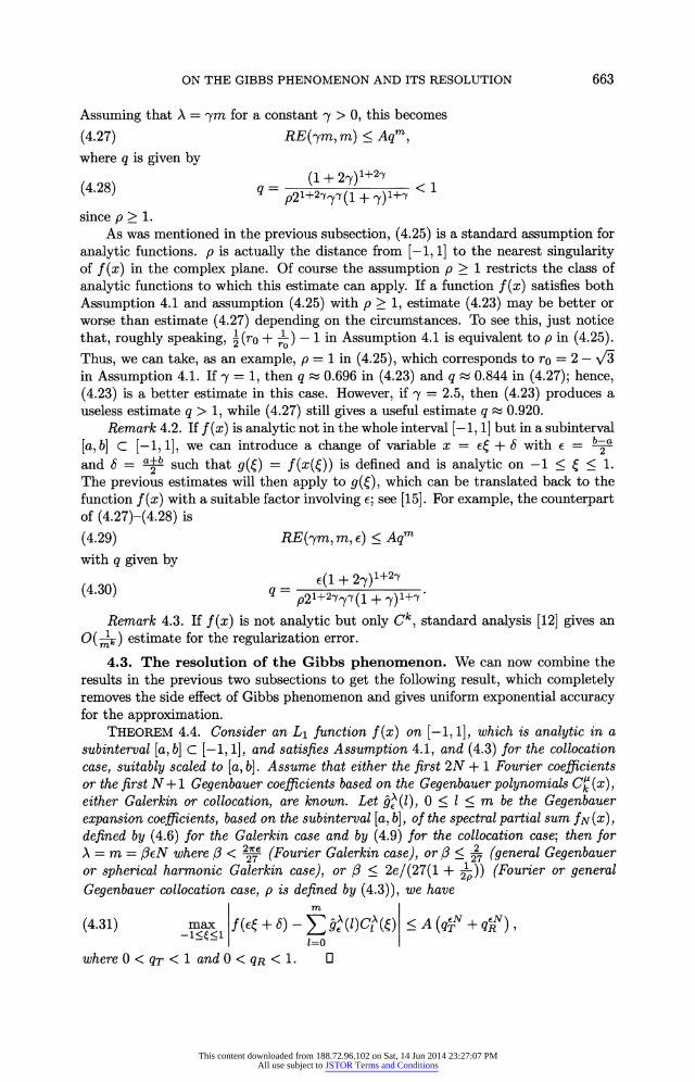
FIG. 1. The function f(x) = x (solid line), the Fourier partial sum fN(x) with N = 4 (short dashed line) and N = 8 (dotted line), and the approximation through the Gegenbauer procedure using m = A = N/4 for N = 4 (long dashed line). Reprinted from Journal of Computational and Applied Mathematics, 43/1-2, D. Gottlieb, C.-W. Shu, A. Solomonoff, and H. Vandeven, On the Gibbs phenomenon I: Recovering exponential accuracy from the Fourier partial sum of a nonperiodic analytic function, pp. 81-98, 1992 with kind permission from Elsevier Science - NL, Sara Burgerhartstraat 25, 1055 KV Amsterdam, The Netherlands.

We return now to problems outlined in the introduction. Theorem 4.4 answers directly Problems 1 and 3. Problems 4 and 5 can be solved by constructing the trigonometric interpolation polynomial and then applying the procedure outlined above using Theorem 4.4. To solve Problem 6 we construct the interpolation polynomial based on the Gauss (or Gauss-Lobatto) points and then apply the procedure outlined above.

5. Numerical examples. An advantage of the procedure described in the previous section is that it is computationally effective even for small N. There are numerical examples given in, e.g., [13, 14, 16, 17, 31, 7, 34, 35]. Some of the numerical difficulties due to round-off errors are addressed in [34]. We will show three samples in this section to illustrate the theory.

The first is the original Gibbs phenomenon as presented by Michelson in [27]: given the first 2N + 1 Fourier coefficients of the analytic but nonperiodic function f (x) = x, find an approximation to f (x) itself. In Figure 1, taken from [13], we can see that the Fourier series fN(x) with N = 4 and N = 8 gives poor approximations throughout the domain and a Gibbs overshoot near the discontinuity. The solution obtained by the Gegenbauer procedure gives excellent results even for the small N = 4.

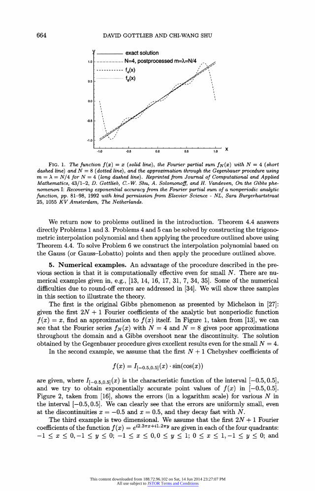
In the second example, we assume that the first N + 1 Chebyshev coefficients of

f (X) = I[_o.5,0.5] (X) * sin(cos(x))

are given, where I[o0.5,0.5] (x) is the characteristic function of the interval [-0.5, 0.5], and we try to obtain exponentially accurate point values of f(x) in [-0.5,0.5]. Figure 2, taken from [16], shows the errors (in a logarithm scale) for various N in the interval [-0.5,0.5]. We can clearly see that the errors are uniformly small, even at the discontinuities x = -0.5 and x = 0.5, and they decay fast with N. - The third example is two dimensional. We assume that the first 2N + 1 Fourier coefficients of the function f (x) = ei2.3-x+i1.2rY are given in each of the four quadrants: -1 < x < O,-1 < y < 0; -1 < x < 0,0 < y < 1; 0 < x < 1,-i < y < 0 and




10-' N=2 1024

106

10-7

io.8 1'?4 N=16 10g

lo10"

12 oX2

lot3r

-0.4 -0.2 0.0 0.2 0.4 0.6

FIG. 2. Errors in log scale, for f(x) = I[0.5,0.5](X) sin(cos(x)), through the Gegenbauer procedure, with N = 20,40,80, 160. Reprinted from D. Gottlieb and C.- W. Shu, On the Gibbs phenomenon V: Recovering exponential accuracy in a sub-interval from the Gegenbauer partial sum of a piecewise analytic function, Mathematics of Computation, 64 (1995), pp. 1081-1095 with permission from the American Mathematical Society.

1.0 ~~~~~~~~~~~~~~~~~~~~~~~~1.0

0.5 ~~~~~~~~~~~~~~~~~~~~~~~~0.5

0.0 ~~~~~~~~~~~~~~~~~~~~~~~~0.0

-0.5 ~~~~~~~~~~~~~~~~~~~~~~~~~-0.5

-1.0 ~~~~~~~~~~~~~~~~~~~~~~~~~-1.0L -1.0 -0.5 0.0 0.5 1.0 -1.0 -0.5 0.0 0.5 1.0

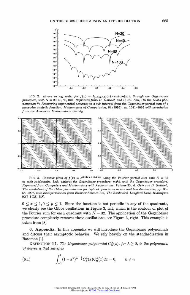
FIG. 3. Contour plots of f (x) = ei2.3rx?+i1 .27Y using the Fourier partial sum with N = 32 in each subdomain. Left, without the Gegenbauer procedure; right, with the Gegenbauer procedure. Reprinted from Computers and Mathematics with Applications, Volume 33, A. Gelb and D. Gottlieb, The resolution of the Gibbs phenomenon for 'spliced' functions in one and two dimensions, pp. 35- 58, 1997, with kind permission from Elesvier Science Ltd, The Boulevard, Langford Lane, Kidlington 0X5 1GB, UK.

O < x < 1, 0 < y < 1. Since the function is not periodic in any of the quadrants, we clearly see the Gibbs oscillations in Figure 3, left, which is the contour of plot of the Fourier sum for each quadrant with N = 32. The application of the Gegenbauer procedure completely removes these oscillations; see Figure 3, right. This example is taken from [8].

6. Appendix. In this appendix we will introduce the Gegenbauer polynomials and discuss their asymptotic behavior. We rely heavily on the standardization in Bateman [1].

DEFINITION 6.1. The Gegenbauer polynomial C>(x), for A > 0, is the polynomial of degree n that satisfies

(6.1) j( - _2 k)A CkIk(x)Cn(x)dx = 0, k 7& n




and is normalized by

(6.2) CA (j) = r(n +2A) -n!r(2 A)

The Gegenbauer polynomials thus defined are not orthonormal. In fact, the norm of C>(x) is given by

(6.3) L -x2)AA (C>(x)) dx = h, -1~~~~~~~~n

where

(6.4) hA = r2C() F(+2) n 1 C"('F(A)(n +A)'

The Gegenbauer polynomials achieve their maximum at the boundary

(6.5) ICn(x)I < C>(1), -1 < x < 1.

In order to study the asymptotics of the Gegenbauer polynomials for large n and A, we will use heavily the well-known Stirling formula: for any number x > 1 we have

(6.6) (2ir)2xX+ 2e-x < r(x + 1) < (2Xr)2X+ 2eXe 12:x.

The first useful fact is that, for large A and n, hA and C>(1) are almost of the same size: there exists a constant A independent of A and n such that

(6.7) A1 A CA(1) hA < A A (n +A) n-( )C"1

which is easily provable from (6.4) and the Stirling formula (6.6). We would also like to quote the Rodrigues formula [1, page 175], which gives an

explicit expression for Cn (X):

(6.8) (1 - )2 Cn() = G(A,n)dTj [(1 - x2)n ,

where G(A, n) is given by

(6.9) G(A, n) - (-1)F(+2)F() + 2) 2nn!r(2A)r(n +A +

Given a function f(x) defined on [-1, 1], its Gegenbauer coefficients fA (1) are defined by

(6.10) fA () = f j( -x2)AAf(x) Ci' (x) dx

with h0 given by (6.4), and the Gegenbauer expansion based on the first m + 1 terms is defined by

m

(6.11) fmA(x) = >3fA(l)CI (X). 1=0




Acknowledgments. We would like to thank Gilbert Strang for many comments on the manuscript and for pointing out that the Vandeven filter (3.32) is essentially the Daubechies filter leading to wavelets. We also thank the American Mathemat- ical Society and the Elsevier Science Publishing Company for giving permission to reproduce the figures.

REFERENCES

[1] H. BATEMAN, Higher Transcendental Functions, Vol. 2, McGraw-Hill, New York, 1953. [2] M. BOCHER, Introduction to the theory of Fourier's series, Ann. Math., 7 (1906), pp. 81-152. [3] H. CARSLAW, A historical note on Gibbs' phenomenon in Fourier's series and integrals, Bull.

Amer. Math. Soc., 31 (1925), pp. 420-424. [4] R. COOK, Gibbs's phenomenon in Fourier-Bessel series and integrals, Proc. London Math.

Soc., 27 (1928), pp. 171-192. [5] R. COOK, Gibbs's phenomenon in Schlomlich series, J. London Math. Soc., 4 (1928), pp. 18-21. [6] The Encyclopedia Britannica, 11th ed., Vol. 4, 1910. [7] A. GELB, The resolution of the Gibbs's phenomenon for spherical harmonics, Math. Comp.,

66 (1997), pp. 699-717. [8] A. GELB AND D. GOTTLIEB, The resolution of the Gibbs's phenomenon for "spliced" functions

in one and two dimensions, Comput. Math. Appl., 33 (1997), pp. 35-58. [9] J. GIBBS, Fourier's series, letter in Nature, 59 (1898), p. 200.

[10] J. GIBBS, Fourier's series, letter in Nature, 59 (1899), p. 606. [11] D. GOTTLIEB, Spectral methods for compressible flow problems, in Lecture Notes in Phys. 218,

Springer-Verlag, New York, 1984, pp. 48-61. [12] D. GOTTLIEB AND S. ORSZAG, Numerical Analysis of Spectral Methods: Theory and Appli-

cations, CBMS-NSF Regional Conference Series in Applied Mathematics, Vol. 26, SIAM, Philadelphia, 1977.

[13] D. GOTTLIEB, C.-W. SHU, A. SOLOMONOFF, AND H. VANDEVEN, On the Gibbs phenomenon I: Recovering exponential accuracy from the Fourier partial sum of a nonperiodic analytic function, J. Comput. Appl. Math., 43 (1992), pp. 81-92.

[14] D. GOTTLIEB AND C.-W. SHU, Resolution properties of the Fourier method for discontinuous waves, Comput. Methods Appl. Mech. Engrg., 116 (1994), pp. 27-37.

[15] D. GOTTLIEB AND C.-W. SHU, On the Gibbs phenomenon III: Recovering exponential accuracy in a subinterval from the spectral partial sum of a piecewise analytic function, SIAM J. Numer. Anal., 33 (1996), pp. 280-290.

[16] D. GOTTLIEB AND C.-W. SHU, On the Gibbs phenomenon IV: Recovering exponential accuracy in a subinterval from the Gegenbauer partial sum of a piecewise analytic function, Math. Comp., 64 (1995), pp. 1081-1095.

[17] D. GOTTLIEB AND C.-W. SHU, On the Gibbs phenomenon V: Recovering exponential accuracy from collocation point values of a piecewise analytic function, Numer. Math., 71 (1995), pp. 511-526.

[18] D. GOTTLIEB AND E. TADMOR, Recovering pointwise values of discontinuous data with spectral accuracy, in Progress and Supercomputing in Computational Fluid Dynamics, Proceedings of US-Israel Workshop, Birkhiiuser-Boston, Cambridge, MA, 1984, pp. 357-375.

[19] A. GRAY AND M. PINSKY, Gibbs phenomenon for Fourier-Bessel series, Exposition Math., 11 (1993), pp. 123-135.

[20] E. HEWITT AND R. HEWITT, The Gibbs-Wilbraham phenomenon: An episode in Fourier analysis, Hist. Exact Sci., 21 (1979), pp. 129-160.

[21] F. JOHN, Partial Differential Equations, Springer-Verlag, Berlin, New York, 1982. [22] C. LANCZOS, Discourse on Fourier Series, Hafner Publishing Company, New York, 1966. [23] G. G. LORENTZ, Approximation of Functions, Holt, Rinehart and Winston, New York, 1966. [24] A. LOVE, Fourier's series, letter in Nature, 58 (1898), pp. 569-570. [25] A. LOVE, Fourier's series, letter in Nature, 59 (1898), pp. 200-201. [26] A. LOVE, Fourier's series, letter in Nature, 60 (1899), pp. 100-101. [27] A. MICHELSON, Fourier series, letter in Nature, 58 (1898), pp. 544-545. [28] A. MICHELSON, Fourier's series, letter in Nature, 59 (1898), p. 200. [29] A. MICHELSON, Fourier's series, letter in Nature, 60 (1899), p. 52. [30] A. MICHELSON AND S. STRATTON, A new harmonic analyser, Philosophical Magazine, 45

(1898), pp. 85-91. [31] C.-W. SHU AND P. WONG, A note on the accuracy of spectral method applied to nonlinear

conservation laws, J. Sci. Comput., 10 (1995), pp. 357-369.




[32] G. STRANG AND T. NGUYEN, Wavelets and Filter Banks, Wellesley-Cambridge Press, Welles- ley, MA, 1996.

[33] H. VANDEVEN, Family of spectral filters for discontinuous problems, J. Sci. Comput., 8 (1991), pp. 159-192.

[34] L. Vozovoi, M. ISRAELI, AND A. AERBUCH, Analysis and application of Fourier-Gegenbauer method to stiff differential equations, SIAM J. Numer. Anal., 33 (1996), pp. 1844-1863.

[35] L. Vozovoi, A. WEILL, AND M. ISRAELI, Spectrally accurate solution of non-periodic differential equations by the Fourier-Gegenbauer method, SIAM J. Numer. Anal., 34 (1997), pp. 1451-1471.

[36] H. WEYL, Die Gibbssche Erscheinung in der Theorie der Kugelfunktionen, Gesammeete Ab- handlungen, Springer-Verlag, Berlin, 1968, pp. 305-320.

[37] H. WILBRAHAM, On a certain periodic function, Cambridge and Dublin Math. J., 3 (1848), pp. 198-201.

[38] J. WILTON, The Gibbs phenomenon in series of Schlomlich type, Messenger of Math., 56 (1926), pp. 175-181.

[39] J. WILTON, The Gibbs phenomenon in Fourier-Bessel series, J. Reine Angew. Math., 159 (1928), pp. 144-153.



on the gibbs phenomenon and its resolution

Documents