INFORMATION AND CONTROL 44, 223-235 (1980)

On the Discrete Time-Optimal Regular Control Problem

M. M. FAHMY

Electrical Engineering Department, Assiut University, Assiut, Egypt

AND

A. A. R. HANAFY AND M. F. SAKR

Electrical Engineering Department, Cairo University, (_h'za, Egypt

This paper considers the time-optimal regulator control of linear discrete multiple-input systems. A new algorithm for realizing the optimal control law is proposed. The feedback gain matrix is expressed in compact closed-form which does not require a recursive solution as in earlier approaches. Numerical examples are worked out to illustrate the procedure.

I . INTRODUCTION

Consider a linear t ime-invariant discrete system governed by the vector- matr ix difference equation

x ( k i l) = ,~l~(k) + Bu(J~), ( l )

where x(k) e R ~ is the state vector and u(k) ~ R ~ is the control vector at the kth iteration, A e R ~x~ is the system matrix, and B ~ R ~'x~ is the control matr ix with r linearly independent columns. The system is assumed to be completely controllable, and its equi l ibr ium state is at the origin in state space.

T h e t ime-opt imal regulator control problem is defined as synthesizing a controller which drives the system (1) from any arbitrary initial state x(0) to the orgin in a min imum number of control iterations. The t ime-optimal closed-loop control law is expressible as a constant linear function of the current state, i.e.,

u(h) - - Fx(k), (2)

where F ~ R ~×" is the feedback gain matrix vet to be determined. Mullis (1972) verified that such an F exists; the solution is generally nonunique. The optimally controlled system is then characterized by the homogeneous form

x(k + 1) := (A t- BF) x(k) (3) and

x(k) .... (A ,- BF)';x(O) (4)

is the t ime-optimal trajectory from x(0) to the origin.

223 0019-9958/801030223-13802.00/0

Copyright ~) 1980 by Academic Press, Inc. All rights of reproduction in any form reserved.

224 FAHMY, IIANAFY~ AND SAKR

Special cases of this problem have been studied earlier. Tou (1964) presented two different methods. The first one (transformation of coordinates) is applicable only to systems with nonsingular matrix .4. The second (iterative design) was developed under the conditions: .4 is nonsingular and the ratio n/r is an integcr. Moreover, it was tacitly assumed that the system can be taken from any x(0) to the origin in n/r steps. We emphasizc that even when n/r is an integer, it may not be possible for the system to reach the origin in n/r steps.

Cadzow (1968) suggested an algebraic method and discussed, further, the properties of the resulting solution in terms of matrix nilpotency and eigen- vectors. His approach is, however, restricted to the case of single-input systems (r == 1) with nonsingular A.

Farison and Fu (1970) investigated the solution as devised by Tou (1964) and arrived at the nilpotcncy property and the Jordan canonical form of the regulator state-transition matrix.

Mullis (1972) treated the problem as posed here: a multiple-input system wi th rank (A) ~ n and rank (B) = r. Nevertheless, the algorithm concluded is generally based on a recursive solution each step of which requires mani- pulation of large matrices. This appreciably increases the computational effort especially when the value of the controllability index is large.

The same problem has also been studied in a recent paper by Sebakhy and Abdel-Moncim (1979). The feedback control law is constructed by solving a sequence of algebraic linear equations. The method is, however, tedious and suffers from the drawbacks of an iterative solution.

In the following sections we take an alternative approach. The minimum-time control problem is formulated as a dual conccpt of the minimum-time observa- tion problem considered by Nagata et al. (1975); see also Fahmy et al. (1979). The optimal feedback gain matrix is expressed in compact closed-form which does not require any recursive or interative steps. Some preliminaries arc given in Section 2 leading up to the actual development of the solution. Section 3 includes the main results and Section 4 demonstrates the procedure with numerical examples.

2. PRELIMINARIES

To begin with, we define the terms "controllability index" and "controllabi- lity matrix" as follows.

DEFINITION 1. The controllability index of the system (1) is defined as the smallest positive integer v : : v,: (~.n) for which

Range [A v] C Range [B, A B ..... Av-'B] (5)

DISCRETE TIME-OPTIMAL PROBI.EM 225

or, equivalently,

Null[A '~] D Null B - f • , ( 6 )

[ B ' A ' " 1

where Range [-] and Null ['] denote the range space and null space, respectively, and the prime (') denotes transposition.

Relation (5) is a necessary and sufficient condition for the system (I) to be completely controllable (Dorato and Levis, 1971).

DEFINITION 2. The controllability matrix S of the system (I) is defined as

S = [B, A B , . . . . . 4"c-~B] . (7)

The matrix S possesses, in general, m (r :::~ m :--'..-~ n) linearly independent vectors among its r ' v , , columns. In our derivation we shall assume for simplicity that m = n. However, the extension of the arguments to the case m < n is a relatively easy task and is outlined at the end of Section 3.

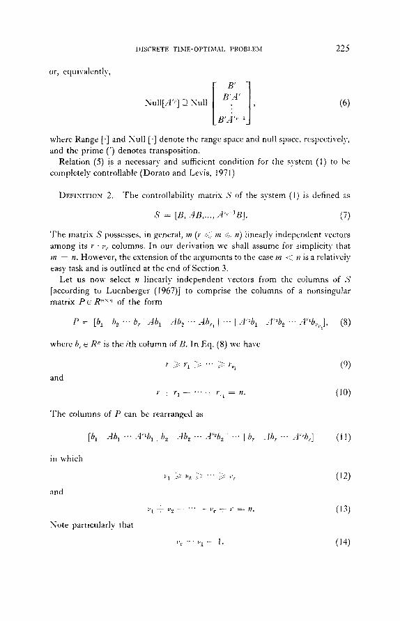
Let us now select n linearly independent vectors from the columns of S [according to Lucnberger (1967)] to comprise the columns of a nonsingular matrix P ~ R ''×'' of the form

. . . , v I - v ! P = [I, 1 11,, . . . b,. A J1.) z .4b., . . . . 4 b r , i "" I A % , .4 bo . . . A b%], (8)

whc,e b i ~ R " is the/ th column (fiB. In Eq. (8) we have

" > rl > ' " ; ' : ;'~1 (9)

and

r • 7" 1 - 7 . . . . ; , q = n . ( 1 0 )

The columns of P can be rearranged as

[b 1 A b 1 " A " ' b 1 I b.,. A b 2 " . , 4 % 2 . . I b , A< . . . A % , . ] (1 l )

in which

and

Note particularly that

v, 2~ v,, ~;7~ " ' " ~7~ vr ( 1 2 )

,21 ~ - :v2 . . . . . . . .v r - 7 - F : : H o (13)

:,~ " q : I . ( 1 4 )

226 FAHMY, HANAFY, AND SAKR

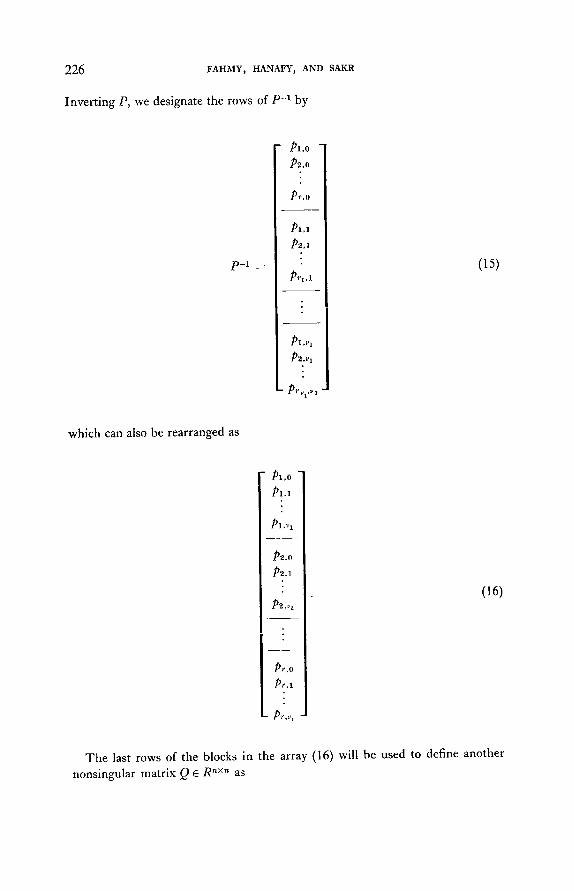
Inverting P, we designate the rows of p--1 by

PI,O " /)2,0

/)r,[)

/)1,1 /)2,l

p - I ~ :

Pri,1

: Pl,vl I

( 1 5 )

which can also be rearranged as

Pl,O

P!.I

Pl,v

/)2.4] /)2.1

)2.v

l )r ,O /).r.l

p.r ,vr •

(16)

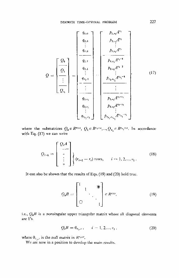
The last rows of the blocks in the array (16) will be used to define another nonsingular matrix Q ~ R ~×n as

DISCRETE TIME-OPTIMAL PROBLEM 227

O __

-Qo]

91 ]

:1]

ql,O

q$,o

q r , o

ql . l

92 ,1

qrl.1

ql,v]

qz.vl

qrv l ,~

p ~v 1 1,v 1

/1 v° P 2 , v "

P l ,Vl~t/vl-I

A V e --I .Prl,V~.l~ I

pt,~, A ~-~'~

prvl WrVlAvrvl -vl

(17)

where the submatr ices Qo ~ R rxn, 01 ~ R,'I×,, 0 E Rr"~ x'~. In accordance

with Eq . (17) we can write

Qi-1 " - I (ri_ t - - r i )rows, i == 1,2,. .• , v x .

(18)

I t can also be shown that the results of Eqs. (19) and (20) hold true.

1

Qo B = ~ R r×', (I 9)

i.e., Qo B is a nonsingular upper t r iangular matr ix whose all diagonal e lements are l ' s .

QiB = 0~,.r, i == 1, 2 ..... vl , (20)

where 0 , . , is the null matr ix in R r~xr.

We are now in a posit ion to develop the main results•

228 FAHMY, HANAFY, AND SAKR

3. ~/IAIN RESULTS

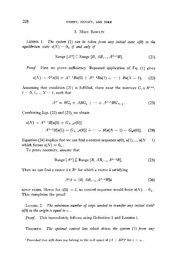
LEMlVIA 1. The system (1) can be taken f r o m any initial state x(O) to the equilibrium state x ( N ) := O~ i f and only i f

P, ange [A -~'] ~ Range [B, AB, . . . , AN-1B]. (21)

Proof. First we prove sufficiency. Repeated application of Eq. (l) gives

x(2\ :) ~= A'Vx(O) + A .v 1Bu(O) + A." 2Bu(1) ~- .. . . L B u ( N - - 1). (22)

Assuming that condition (21) is fulfilled, there exist the matrices GiE R '×'~, i - 0, 1 ..... N - - l, such that

A "v -- BGo + A B G 1 1 . . . . + A 'V- IBGN-1- (23)

Combining Eqs. (22) and (23), we obtain

x ( N ) = .4." 1B[u(0) + G~. ,x(0)]

: AX-2B[u(1) + G,v_2x(O)] + . . . . i- B [ u ( g - l) + Gox(0)]. (24)

Equation (24) implies that we can find a control sequence u(0), u(l),..., u ( N - - 1) which forces x ( N ) = 0,, .

To prove necessity, assume that

Range [A-"] ~ Range [B, AB, . . . , A'V-XB]. (25)

Then we can find a vector a~ e R" for which a vector ~ satisfying

A"0~ - : [B, A B ..... A " - ' B ] ~ (26)

never exists. Hence for x(0) := ,~, no control sequence would force x ( N ) := O~ . This completes the proof.

I,rMMA 2. The minimum number of steps needed to transfer any initial state t

x(O) to the origin is equal to v,. .

Proof. This immediately follows using Definition 1 and Lemma 1.

THEOREM. The optimal control law which drives the system (1)front an 3,

x Provided that x(0) does not belong to the null space of (A + BF) ~ for v <,~ v~ .

DISCRETE "rIME-OP'n.~LaL PROBLEM 2 2 9

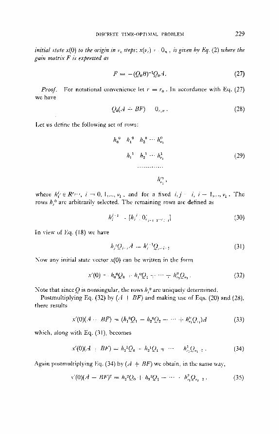
initial state x(O) to the origin in ,,,, steps; x(v,.) = 0~ , is given by Eq. (2) where the gain matrix F is expressed as

Proof.

F . . . . . (QoB)- 'QoA. (27)

For notat ional convenience let r = r o . In accordance with Eq. (27)

o,.,. (28)

hi ° h2°...h{Jl

hi 1 h2 t "- h~,

h'q

we h a v e

Q . 0 4 - - - B F )

l int us define the following set of rows:

ho °

(29)

where h~" e R ..... , i = 0, I ..... v 1 , and for a fixed i , j : i, i -c 1,..., v 1 . T h e rows hfl arc arbitrarih, selected. T h e remain ing rows are defined as

h i " - [ h / : 0 ; , _ , ,__,..,] (30)

In view of Eq. (18) we have

h/(.)j_iA -~ h~"Q~_i_., (31)

Now any initial statc vcctor x(0) can be writ ten in the form

[I x ' ( o ) = hoOQo , h , ° Q , -, . . . . . _ s,~. C), . (32)

Note that sincc Q is nonsingular , thc rows hfl are un ique ly determined.

Pos tnml t ip ly ing Eq. (32) by (,,J ! BF) and making usc of Eqs. (20) and (28), there results

x ' ( 0 ) ( A - i B F ) =-- (lh°Q, = h2°Q2 . . . . . . . ~- h~'Q,.,)A (33)

which, along with Eq. (31), bccomes

x ' (O)(A : B F ) = / q J Q o -- 1,2'f...)~ ~ - ' hJ/_.),., .~ . (34)

Again pos tmul t ip ly ing l 'q. (34) by (A -p BF) we obtain, in the same way,

.~'(0)(.4 - - BF) ~ = I",'-'C),, i-h,~2Q~ . . . . . I h~,Q,,, ~. (35)

230 FAHMY, H.MNAFY, AND SAKR

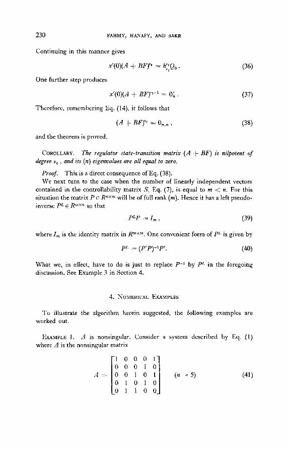
Continuing in this manncr gives

x'(O)(A ~- BF) vl == h;1Qo .

One further step produces

x'(O)(A + BF) ~,'1 _~ On.

Therefore, remembering Eq. (14), it follows that

(A + BF) . . . . . 0 . . . .

and the theorem is proved.

(36)

(37)

(38)

COROLLARY. The regulator state-transition matrix ( A . ~- BF) is nilpotent of degree vc , and its (n) eigenvalues are all equal to zero.

Proof. This is a direct consequence of Eq. (38). We next turn to the case when the number of linearly independent vectors

contained in the controllability matrix S, Eq. (7), is equal to m < n. For this situation the matrix P 6 R È×m will be of full rank (m). Hence it has a left pseudo- inverse pL ~ R,,xr, so that

p L p .= I n , (39)

where I,~ is the identity matrix in R "`xm. One convenient form of pL is given by

p,. := (p ,p ) - l p , . (40)

What we, in effect, have to do is just to replace p - t by pi. in the foregoing discussion. See Example 3 in Section 4.

4. ~UMERICAI, EXAMPI.ES

T o illustrate the algorithm herein suggested, the following examples are worked out.

EXAMPLE 1. A is nonsingular. Consider a system described by Eq. (1) where A is the nonsingular matrix

0 0 0 1 .4 =- 0 0 1 0 (n = 5) (41)

l 0 1 1 1 0

DISCRETE TIME-OPTIMAL PROBI.EM 231

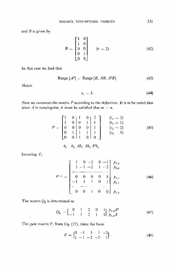
and B is given by

l Z] R= ~ ~r=2) ~42)

In this case we find that

Hence

Range [A a] - : Range [B, A B, A2B]. (43)

vc -- 3. (44)

Now we construct the matrix P according to the definition. It is to be noted that since A is nonsingular, it must be satisfied that m ..= n.

P .....

Ii ° 0 0 l 0

1 0 0 1 0 0 [ 1 1 0

1:1, 2 =-~) =-.1) (vl ---2) (,,., ~ 1)

(45)

bl b2 Abl ,4b2 A"bl

Inverting P,

p . l = .

I 0 - - 2 0 - - 1 - 1 - -1 - - 2 1 - - 2

0 0 0 0 1 - -1 1 1 0 1

0 0 1 0 0

Pl ,o P2,o

Pi.1 P2,1

Pl.o_

(46)

The matrix Qo is determined as

[ o 1 2 o lt]p,.2A'-' Qo '= - 1 1 2 1 p,~,lA (47)

The gain matrix F, from Eq. (27), takes the form

[0 _l _3 _, ~ ] ~48) F .... 1 - - I - - 2 - - 2 "

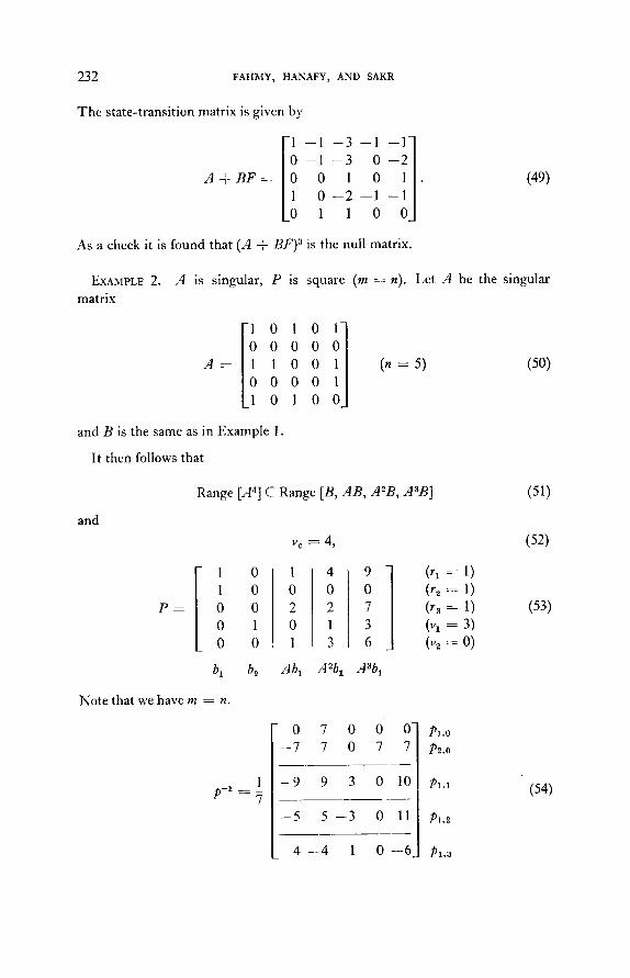
232 FAHMY, HANAFY, AND SAKR

The state-transition matrix is given by

A -~- BF=:

133 l 0 0 1 0 . 0 - - 2 --1 - - 1 1 0

As a check it is found that (A + BF) :~ is the null matrix.

EXAMPLE 2. A is singular, P is square (m --: n).

matrix

0 0 0 A : 1 0 0 (n - - 5)

0 0 0 0 1 0

and B is the same as in Example 1.

I t then follows that

and

Range [A 4] C Range [B, AB, A2B, A3B]

vc = 4,

P =

1 0 1 0 0 0 0 1 0 0

bl b.z

1 0 2 0 1

Aba

4 0 2 1 3

A2bl

0 7 3 6

ASbl

Note that we have m = n.

1 p-1 =

0 7 0 0 0- - -7 7 0 7 7

- 9 9 3 0 l0

- -5 5 - -3 0 11

4 - - 4 1 0 - - 6

(49)

Let A be the singular

(50)

(51)

(52)

( r I =: 1) (r 2 := 1) ( r 3 - - 1 ) (53)

(Vl = 3) (v~:= 0)

Pl ,o

/'2,0

P1,1 (54)

DISCRETE TIME-OPTIMAl'. PROBLE3,'I 233

1[ 3 4 - 1 0 67]Pl'aA~ (55) Qo - ~ - 7 7 0 7 P.,_,o

I [--8 1 --9 0 --~] (56) F- -~ 0 0 0 0

. - 1 - 9 0 - - _ 1 7 0 0 ( 5 7 )

A B F = ~ 0 0 0

0 7 0

To check, (A - BF) 4 is the null matrix.

~XA1MPLE 3. matrix

A is nilpotent, P is rectangular (m < n). I,et A be the nilpotent

! 0 0 0 A = 0 0 0 0 (n .... 5)

0 0 0 0 0 0

(5s)

and B is again as in Example 1. Here we have

Range [A 'a] C Range [B, AB] (59)

and

v~. = 2, (60)

P _

I I 0 1 0 0 0 0 1 0 0

b 1 b.,

0 1

0 0 0

Ab~

(r 1 1 ) (~, =-1) (,,,, :--: o) (61)

Note that 1;, : 3. From Fq. (40) we get

p£ = I l 0

- 1

o,F 0 0 0 0 Pt.o 0 0 1 P".o

-( Pl. t l 0 0 _

(62)

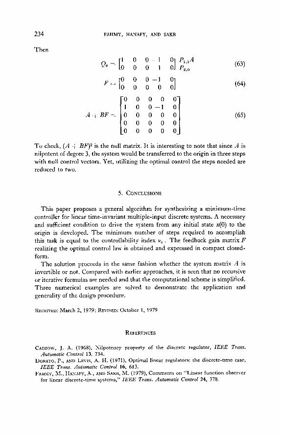
234 FAHMY, HANAFY, AND SAKR

Then

[1 0 0 - - 1 00] PI,xA (63) Qo = 0 0 0 1 P2,o

[0 0 0 -- 1 0] (64) F : ~ 0 0 0 0 0 [ ooo 1 0 0 - - 1

A + B F =~ 0 0 0 (65) 0 0 0 0 0 0

T o check, (A -i B F ) 2 is the null matrix. I t is interesting to note that since d is nilpotent of degree 3, the system would be transferred to the origin in three steps with null control vectors. Yet, utilizing the optimal control the steps needed are reduced to two.

5. CONCLUSIONS

This paper proposes a general algorithm for synthesizing a minimum-t ime controller for lincar time-invariant multiple-input discrete systems. A necessary and sufficient condition to drive the system from any initial state x(0) to the origin is devcloped. T h e min imum number of steps rcquired to accomplish this task is equal to the controllability index v~.. The feedback gain matrix F realizing the optimal control law is obtained and expressed in compact closed- fo rm.

T h e solution proceeds in the same fashion whethcr thc system matrix A is invertible or not. Compared with earlier approaches, it is scen that no recursive or iterative formulas are needed and that the computational scheme is simplified. Three numerical examples are solved to demonstratc the application and generality of the design procedure.

RECEIVED: March 2, 1979; REVISED: October 1, 1979

REFERENCES

CADZOW, J. A. (1968), Nilpotency property of the discrete regulator, IEEE Trans. Automatic Control 13, 734.

DOaATO, P., AND LEVIS, A. H. (1971), Optimal linear regulators: the discrete-time case, 1EEE Trans. Automatic Control 16, 613.

FAH.~tV, M., HA-~AFY, A., AND SAKR, M. (1979), Comments on "Linear function observer for linear discrete-time systems," 1EEE Trans. Automatic Control 24, 378.

DISCRETE TIME-OPTIMAL PROBLF.M 235

FARISON, J. B., AND FL', F. C. (1970), The matrix properties of minimum-time discrete linear regulator control, IEEE Trans. Automatic Control 15, 390.

LUENBERCER, D. G. (1967), Canonical forms for linear multivariable systems, I E E E Trans. Automatic Control 12, 290.

IX'IULLIS, C. T. (1972), Time optimal discrete regulator gains, IEEE Tram'. Automatic Control 17, 265.

NAGATA, A., NISHIMURA, T., AND IKEDA, M. (1975), Linear function observer for linear discrete-time systems, I E E E Trans. Automatic Control 20, 401.

SEBAKHY, O. A., AND ABDEI.-]VIoNEIM, T. M. (1979), State regulation in linear discrete- time systems in minimum time, I E E E Trans. Automatic Control 24, 84.

Tou, J. T. (1964), "Modern Control Theory," p. 155, McGraw-Hill, New York.