on the complexity of steepest descent, newton’s and ... · on the complexity of steepest descent,...

On the complexity of steepest descent, Newton’s and

regularized Newton’s methods for nonconvex

unconstrained optimization

C. Cartis, N. I. M. Gould and Ph. L. Toint

15 October 2009

Abstract

It is shown that the steepest descent and Newton’s method for unconstrainednonconvex optimization under standard assumptions may be both require a numberof iterations and function evaluations arbitrarily close to O(ǫ−2) to drive the normof the gradient below ǫ. This shows that the upper bound of O(ǫ−2) evaluationsknown for the steepest descent is tight, and that Newton’s method may be as slowas steepest descent in the worst case. The improved evaluation complexity bound ofO(ǫ−3/2) evaluations known for cubically-regularised Newton methods is also shownto be tight.

1 Introduction

We consider the numerical solution of the unconstrained (possibly nonconvex) optimizationproblem

minxf(x) (1.1)

where we assume that f : IRn → IR is twice continuously differentiable and bounded below.All practical methods for the solution of (1.1) are iterative and generate a sequence {xk}of iterates approximating a local minimizer of f . A variety of algorithms of this form exist,amongst which the steepest-descent and Newton method are preeminent.

At iteration k, the steepest descent method chooses the new iterate xk+1 by minimiz-ing (typically inexactly) f(xk − tgk), for t ≥ 0, where gk = ∇xf(xk). This first-ordermethod has the merit of simplicity and a theoretical guarantee of convergence under weakconditions (see Dennis and Schnabel, 1983, for instance). The number of iterations re-quired in the worst case to generate an iterate xk such that ‖gk‖ ≤ ǫ (for ǫ > 0 arbitrarilysmall) is known to be at most O(ǫ−2) (see Nesterov, 2004, page 29), but the question ofwhether this latter bound is tight has remained open. The practical behaviour of steep-est descent may be poor on ill-conditioned problems, and it is not often used for solvinggeneral unconstrained optimization problems.

By contrast, Newton’s method and its variants are popular and effective. At iterationk, this method (in its simplest and standard form) chooses the next iterate by minimizingthe quadratic model

mk(xk + s) = f(xk) + gTk s+ 1

2sT

kHksk, (1.2)

where Hkdef= ∇xxf(xk) is assumed to be positive definite. This algorithm to known

to converge locally and quadratically to strict local minimizers of the objective functionf , but in general convergence from arbtrary starting points cannot be guaranteed, inparticular because the Hessian Hk may be singular or indefinite, making the minimizationof the quadratic model (1.2) irrelevant. However, Newton’s method works surpringlyoften without this guarantee, and, when it does, is usually remarkably effective. Weagain refer the reader to classics in optimization like Dennis and Schnabel (1983) and

1

Cartis, Gould, Toint: Complexity of steepest descent, Newton’s and ARC methods 2

Nocedal and Wright (1999) for a more extensive discussion of this method. To the bestof our knowledge, no worst-case analysis is available for this standard algorithm appliedon possibly nonconvex problems (a complexity analysis is however available for the casewhere the objective function is convex, see Nesterov, 2004, for instance).

Globally convergent variants of Newton’s method have been known and used for along time, in the linesearch, trust-region or filter frameworks descriptions may be found inDennis and Schnabel (1983), of which Conn, Gould and Toint (2000) and Gould, Sainvituand Toint (2005), respectively. Although theoretically convergent and effective in practice,the complexity of most of these variants applied on general nonconvex problems has not yetbeen investigated. The authors are only aware of the analysis by Gratton, Sartenaer andToint (2008), (Corollary 4.10) where a bound on the complexity of an inexact variant of thetrust-region method is shown to be of the same order as that of steepest descent, and of theanalysis by Ueda and Yamashita (2008, 2009) and Ueda (2009), which essentially provesthe same result for a variant of Newton’s method using Levenberg-Morrison-Marquardtregularization.

Another particular globally convergent variant of Newton’s method for the solution ofnonconvex unconstrained problems of the form (1.1) is of special interest, because it iscovered by a better worst-case complexity analysis. Independently proposed by Griewank(1981), Weiser, Deuflhard and Erdmann (2007) and Nesterov and Polyak (2006) andsubsequently adapted in Cartis, Gould and Toint (2009a), this method uses a cubic regu-larization of the quadratic model (1.2) in that the new iterate is found at iteration k byglobally minimizing the cubic model

mk(xk + s) = f(xk) + gTk s+ 1

2sT

kHksk + 1

3σk‖sk‖3, (1.3)

where σk ≥ 0 is a suitably chosen regularization parameters (the various cited authorsdiffer in how this choice is made). This method, which we call the Adaptive Regularizationwith Cubics (ARC) algorithm, has been shown to require at most O(ǫ−3/2) iterationsto produce an iterate xk such that ‖gk‖ ≤ ǫ, provided the objective function is twicecontinuously differentiable, bounded below and provided ∇xxf(x) is globally Lipschitzcontinuous on each segment [xk, xk+1] of the piecewise linear path defined by the iterates.This result, due to Nesterov and Polyak (2006) when the model minimization is global andexact and to Cartis, Gould and Toint (2007) for the case where this minimization is onlyperformed locally and approximately, is obviously considerably better than that for thesteepest-descent method. We note here that even better complexity results in the convexcase are discussed for ARC by Nesterov (2008) and Cartis, Gould and Toint (2009b), andfor other regularized Newton’s methods by Polyak (2009) and Ueda (2009).

But obvious questions remain. For one, whether the steepest descent method mayactually require O(ǫ−2) functions evaluations on functions with Lipschitz continuous gra-dients is of interest. The first purpose of this paper is to show that this is so. The lackof complexity analysis for the standard Newton’s method also raises the possibility that,despite its considerably better performance on problems met in practice, its worst-casebehaviour could be as slow as that of steepest descent. A second objective of this paper isto show that this is the case, even if the objective function is assumed to be bounded belowand twice-continuously differentiable with Lipschitz continuous Hessian on each segmentof the piecewise linear path defined by the iterates. This establishes a clear distinctionbetween Newton’s method and its ARC variant, for which a substantially more favourableanalysis exists. The question then immediately arises to decide whether this better boundfor ARC is actually the best that can be achieved. The third aim of the paper is todemonstrate that it is indeed the best.

The paper is organized as follows. Section 2 introduces an example for which thesteepest descent method is as slow as its worst-case analysis suggests. Section 3 thenexploits the technique of Section 2 for constructing examples for which slow convergenceof Newton method can be shown, while Section 4 further discusses the implications ofthese examples (and the interpretation of of worst-case complexity bounds in general).Section 5 then again exploits the same technique for constructing an example where the


ARC algorithm is as slow as is implied by the aforementioned complexity analysis. Someconclusions are finally drawn in Section 6.

2 Slow convergence of the steepest descent method

Consider using the steepest descent method for solving (1.1). We would like to constructan example on which this algorithm converges at a rate which corresponds to its worst-case on general nonconvex objective functions, i.e. such that one has to perform O(ǫ−2)iterations to ensure that

‖gk+1‖ ≤ ǫ. (2.1)

In order to achieve this goal, a suitable condition is to require that, for all k ≥ 0,

‖gk‖ ≥(

1

k + 1

)1

2

. (2.2)

An arbitrarily close approximation can considered by requiring that, for any τ > 0, New-ton’s method needs O(ǫ−2+τ ) iterations to achieve (2.1), which leads to the condition that,for all k ≥ 0,

‖gk‖ ≥(

1

k + 1

)1

2−τ

. (2.3)

Our objective is therefore to construct sequences {xk}, {gk}, {Hk} and {fk} such that(2.3) holds and which may be generated by the steepest descent algorithm, together witha twice continuously differentiable function f1(x) such that

fk = f1(xk), and gk = ∇xf1(xk) (2.4)

In addition, f1 must be bounded below and Hk must be positive definite for the algorithmto be well-defined. We also would like f1 to be as smooth as possible; we are aiming at

AS.0 f is twice continuously differentiable, bounded below, and has bounded Lipschitzcontinuous gradient,

since these are the standard assumptions under which globalized steepest descent is prov-ably convergent (see Dennis and Schnabel, 1983, Theorem 6.3.3).

Our example is unidimensional and we define, for all k ≥ 0,

x0 = 0, xk+1 = xk + αk

(

1

k + 1

)1

2+η

, (2.5)

for some steplength αk > 0 such that, for constant α and α,

0 < α ≤ αk ≤ α < 2, (2.6)

giving the step

skdef= xk+1 − xk = αk

(

1

k + 1

)1

2+η

. (2.7)

We also set

f0 =1

2ζ(1 + 2η), fk+1 = fk − αk(1− 1

2αk)

(

1

k + 1

)1+2η

, (2.8)

gk = −(

1

k + 1

)1

2+η

, and Hk = 1, (2.9)

where

η = η(τ)def=

1

2− τ −1

2=

τ

4− 2τ> 0 (2.10)


and ζ(t)def=∑∞

k=1 k−t is the Riemann ζ function, which is finite for all t > 1 and thus

for t = 1 + 2η. Immediately note that the first part of (2.9) gives (2.3) by construction.In what follow the choice of αk is arbitrary in the interval [α, α], but we observe that theselected value of αk can be seen as resulting from a Goldstein-Armijo linesearch enforcing,for some α, β ∈ (0, 1) with α < β,

f(xk)− f(xk+1) ≥ −αsTk gk = ααk‖gk‖2 and f(xk)− f(xk+1) ≤ −βsT

k gk = βαk‖gk‖2,

since (2.8) ensures that 2(1− α) < αk < 2(1− β) and thus that (2.6) holds.We now exhibit function f1(x) which satisfies AS.0 and (2.4)-(2.9). For this purpose,

we use polynomial Hermite interpolation on the interval [0, xk+1 − xk], which we willsubsequently translate. We are thus seeking a polynomial of the form

pk(t)def= c0,k + c1,kt+ c2,kt

2 + c3,kt3 + c4,kt

4 + c5,kt5 (2.11)

on the interval [0, µk] (where µk = sk) such that

pk(0) = αk(1− 1

2αk)

(

1

k + 1

)1+2η

, pk(µk) = 0, (2.12)

p′k(0) = −(

1

k + 1

)1

2+η

p′k(µk) = −(

1

k + 2

)1

2+η

, (2.13)

and we also impose that p′′k(0) = p′′k(µk) = 1. These conditions immediately give that

c0,k = αk(1− 1

2αk)

(

1

k + 1

)1+2η

, c1,k = −(

1

k + 1

)1

2+η

and c2,k =1

2.

One then verifies that the remaining interpolation conditions may be written in the form

µ3k µ4

k µ5k

3µ2k 4µ3

k 5µ4k

6µk 12µ2k 20µ3

k

c3c4c5

=

0p′k(µk)

0

,

whose solution turns out to be

c3,k

c4,k

c5,k

=

−4φkµk

7φk

µ2k

−3φk

µ3k

(2.14)

where

φk =1

αk(1− αk − ψk) with ψk

def=

(

k + 1

k + 2

)1

2+η

. (2.15)

The definition of ψk implies that |ψk| ∈ (0, 1) for all k ≥ 0, The function f1 is thenrecursively defined on the nonnegative reals(1) by

f1(x) = pk(x− xk) + fk+1 for x ∈ [xk, xk+1] and k ≥ 0. (2.16)

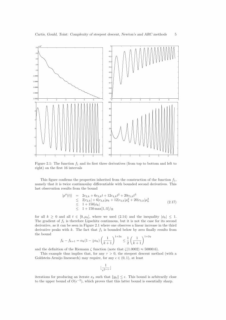
The graph of this function and its first three derivatives are given on the first 16 intervalsand for η = 10−4 and αk = 1 by Figure 2.1.

(1)It can be easily smoothly extended to the negative reals while maintaining its boundedness and thebounded nature of its second derivatives.


0 1 2 3 4 5 6 72.4999

2.4999

2.4999

2.4999

2.4999

2.5

2.5

2.5

2.5

2.5x 10

4

0 1 2 3 4 5 6 7−1

−0.9

−0.8

−0.7

−0.6

−0.5

−0.4

−0.3

−0.2

−0.1

0

0 1 2 3 4 5 6 7−3

−2

−1

0

1

2

3

0 1 2 3 4 5 6 7−60

−40

−20

0

20

40

60

80

100

Figure 2.1: The function f1 and its first three derivatives (from top to bottom and left toright) on the first 16 intervals

This figure confirms the properties inherited from the construction of the function f1,namely that it is twice continuoulsy differentiable with bounded second derivatives. Thislast observation results from the bound

|p′′(t)| = 2c2,k + 6c3,kt+ 12c4,kt2 + 20c5,kt

3

≤ 2|c2,k|+ 6|c3,k|µk + 12|c4,k|µ2k + 20|c5,k|µ3

k

≤ 1 + 150|φk|≤ 1 + 150max[1, α]/α

(2.17)

for all k ≥ 0 and all t ∈ [0, µk], where we used (2.14) and the inequality |φk| ≤ 1.The gradient of f1 is therefore Lipschitz continuous, but it is not the case for its secondderivative, as it can be seen in Figure 2.1 where one observes a linear increase in the thirdderivative peaks with k. The fact that f1 is bounded below by zero finally results fromthe bound

fk − fk+1 = αk(1− 1

2αk)

(

1

k + 1

)1+2η

≤ 1

2

(

1

k + 1

)1+2η

and the definition of the Riemann ζ function (note that ζ(1.0002) ≈ 50000.6).This example thus implies that, for any τ > 0, the steepest descent method (with a

Goldstein-Armijo linesearch) may require, for any ǫ ∈ (0, 1), at least

⌊ 1

ǫ2−τ⌋

iterations for producing an iterate xk such that ‖gk‖ ≤ ǫ. This bound is arbitrarily closeto the upper bound of O(ǫ−2), which proves that this latter bound is essentially sharp.


3 Slow convergence of Newton’s method

Now consider using Newton’s method for solving (1.1). We now would like to construct anexample on which this algorithm converges at a rate which corresponds to the worst-caseknown for the steepest descent method on general nonconvex objective functions, i.e. suchthat one has to perform O(ǫ−2) iterations to ensure (2.1). As above, a suitable conditionfor achieving this goal is to require that (2.2) holds for all k ≥ 0, and an arbitrarily closeapproximation can considered by requiring that, for any τ > 0, Newton’s method needsO(ǫ−2+τ ) iterations to achieve (2.1), leading to the requirement that (2.3) holds for allk ≥ 0. Our current objective is therefore to construct sequences {xk}, {gk}, {Hk} and{fk} such that this latter condition holds and which may now be generated by Newton’salgorithm, together with a twice continuously differentiable function f2(x) such that

fk = f2(xk), gk = ∇xf2(xk) and Hk = ∇xxf2(xk). (3.1)

In addition, f2 must be bounded below and Hk must be positive definite for the algorithmto be well-defined. We also would like f2 to be as smooth as possible; we are aiming at

AS.1 f is twice continuously differentiable, bounded below, and had bounded and Lips-chitz continuous second derivatives along each segment [xk, xk+1],

since these are the standard assumptions under which globalized Newton’s method isprovably convergent (see Dennis and Schnabel, 1983, Theorem 6.3.3, Fletcher, 1987, The-orem 2.5.1, or Nocedal and Wright, 1999, Theorem 3.2).

Our example is bidimensional and we define, for all k ≥ 0,

x0 = (0, 0)T , xk+1 = xk +

(

1k+1

)1

2+η

1

, (3.2)

f0 =1

2[ζ(1 + 2η) + ζ(2)] , fk+1 = fk −

1

2

[

(

1

k + 1

)1+2η

+

(

1

k + 1

)2]

, (3.3)

gk = −

(

1k+1

)1

2+η

(

1k+1

)2

, and Hk =

(

1 0

0(

1k+1

)2

)

(3.4)

where, as in (2.10), η = τ/(4− 2τ) > 0 and ζ(t)def=∑∞

k=1 k−t is the Riemann ζ function.

The first part of (3.4) then immediately gives (2.3) by construction, since the norm of thatvector is at least equal to the absolute value of its first component.

We now verify that, provided (3.1) holds, the sequences given by (3.2)–(3.4) may begenerated by Newton’s method. Defining

skdef= xk+1 − xk =

(

1k+1

)1

2+η

1

def=

(

µk

1

)

(3.5)

and remembering (1.2), this amounts to verifying that

gTk sk + sT

kHksk = 0, (3.6)

Hk is positive definite (3.7)

and thatf(xk + sk) = mk(xk + sk) (3.8)


for all k ≥ 1. Note that, by definition µk ∈ (0, 1]. The first two of these conditions saythat the quadratic model (1.2) is globally minimized exactly. In our case, (3.6) becomes,using (3.5), (3.2) and (3.4),

gTk sk + sT

kHksk = −(

1

k + 1

)1+2η

−(

1

k + 1

)2

+

(

1

k + 1

)1+2η

+

(

1

k + 1

)2

= 0,

as desired, while (3.7) also follows from (3.4). Using (3.3) and (3.4), we also obtain that

mk(xk + sk) = f(xk) + gTk sk + 1

2sT

kHksk

= f(xk)− 12

(

1k + 1

)1+2η

− 12

(

1k + 1

)2

= f(xk+1),

which in turn yields (3.8).We now have to exhibit a function f2(x) which satisfies AS.1 and (3.1)-(3.4). The

above equations suggest a function of the form

f2(x) = f2,1([x]1) + f2,2([x]2)

where [x]i is the i-th component of the vector x and where the univariate f2,1 and f2,2 arecomputed separately. Since our conditions involve, for both functions, fixed values of thefunction

f2,1(0) =1

2ζ(1 + 2η), f2,1([xk+1]1) = f2,1([xk]1)−

1

2

(

1

k + 1

)1+2η

, (3.9)

f2,2(0) = 1/2ζ(2), f2,2([xk+1]2) = f2,2([xk]2)−1

2

(

1

k + 1

)2

, (3.10)

and of its first and second derivatives at the endpoints of the interval [xk, xk+1], we againconsider applying polynomial Hermite interpolation on the interval [0, xk+1−xk], which wewill subsequently translate. Considering f2,1 first, we note that it has to satsify conditionsthat are identical to those stated for f1 in Section 2 for the case where αk = 1 for all k.We may then choose

f2,1([x]1) = f1([x]1).

Let us now consider f2,2. Again, we seek a polynomial

qk(t)def= d0,k + d1,kt+ d2,kt

2 + d3,kt3 + d4,kt

4 + d5,kt5

on the interval [0, 1] such that

qk(0) =1

2

(

1

k + 1

)2

, qk(1) = 0,

q′k(0) = −(

1

k + 1

)2

q′k(1) = −(

1

k + 2

)2

,

q′′k (0) =

(

1

k + 1

)2

and q′′k (1) =

(

1

k + 2

)2

,

These conditions immediately give that

d0,k =1

2

(

1

k + 1

)2

, d1,k = −(

1

k + 1

)2

and d2,k =1

2

(

1

k + 1

)2

.


Applying the same interpolation technique as above, one verifies that

d3,k

d4,k

d5,k

=1

2

9(

1k+2

)2

−(

1k+1

)2

−16(

1k+2

)2

+ 2(

1k+1

)2

7(

1k+2

)2

−(

1k+1

)2

,

yielding in turn that

f2,2([x]2) = qk([x2 − xk]2) + f2,2([xk+1]2) for [x]2 ∈[

[xk]2, [xk+1]2]

and k ≥ 0,

and that|q′′(t)| = 2d2,k + 6d3,kt+ 12d4,kt

2 + 20d5,kt3

≤ 2|d2,k|+ 6|d3,k|+ 12|d4,k|+ 20|d5,k|≤ 1 + 6× 5 + 12× 9 + 20× 4= 219

for all k ≥ 0 and all t ∈ [0, 1].The graph of this function and its first three derivatives are given on the first 16 inter-

vals and for η = 10−4 by Figure 3.2. As for f2,1 = f1, this figure confirms the propertiesinherited from the construction of the function f(x), namely that it is twice continuousdifferentiable and has uniformly bounded second derivative. Its second derivative is nowglobally Lipschitz continuous, as it can be seen in Figure 3.2 where one observes that thethird derivative is bounded above in norm for all k. The fact that f2 is bounded below byzero results from (3.10) and the fact that ζ(2) = π2/6.

0 2 4 6 8 10 12 14 160

0.1

0.2

0.3

0.4

0.5

0.6

0.7

0.8

0.9

0 2 4 6 8 10 12 14 16−1

−0.9

−0.8

−0.7

−0.6

−0.5

−0.4

−0.3

−0.2

−0.1

0

0 2 4 6 8 10 12 14 16−0.2

0

0.2

0.4

0.6

0.8

1

1.2

1.4

0 2 4 6 8 10 12 14 16−3

−2

−1

0

1

2

3

4



0 2 4 6 8 10 12 14 16 18−5

0

5

10

24998.6779

24998.713424998.7134

24998.751924998.7519

24998.7939

24998.7939

24998.8371

24998.8371

24998.888324998.8883

24998.942724998.9427

24998.9427

24999.004824999.0048

24999.0048

24999.07724999.077

24999.077

24999.159324999.1593

24999.1593

24999.256824999.2568

24999.2568

24999.3789

24999.3789

24999.378924999.3789

24999.535124999.5351

24999.535124999.5351

24999.7591

24999.759124999.7591

25000.132125000.1321

25000.13210 1 2 3 4 5 60

5

10

15

Figure 3.3: The third derivative of the function f2(x) along the path [xo, . . . , x16], andthis path on the level curves of f2.

One may also compute the third derivative of f2 along the step, which is given, in thek-th interval, by

1‖sk‖3

[p′′′k (t)(sk)31 + q′′′k (t)] < p′′′k (t)(sk)31 + q′′′k (t)

≤ (6c3,k + 24c4,kt+ 60c5,kt2)µ3

k

+6d3,k + 24d4,kt+ 60d5,kt2

< 6|c3,k|µk + 24|c4,k|µ2k + 60|c5,k|µ3

k

+6|d3,k|+ 24|d4,k|+ 60|d5,k|≤ 6× 4 + 24× 7 + 60× 3 + 6× 5 + 24× 9 + 60× 4= 858,

where we used the inequalities ‖sk‖ > 1 and t ≤ 1 and hence, because of the mean-valuetheorem, f2(x) has Lipschitz continuous second derivatives in each segment of the piecewiselinear path ∪∞k=0[xk, xk+1]. The actual value of the third derivative on the first segmentsof this path is shown on the left side of Figure 3.3, while the path itself is illustrated onthe right side, superposed on the levels curves of f . As a consequence, f2(x) satisfies AS.1,as desired.

If we are now ready to give up smoothness of the objective function beyond continuousdifferentiability, it is then possible to construct an example with τ = η = 0, therebyguaranteeing that Newton’s method takes precisely ǫ−2 iterations to generate ‖gk−1‖ ≤ ǫwhen applied to f3, with a certain x0 and for any ǫ > 0. Thus we relax our asumptions to

AS.2 f is twice continuously differentiable and bounded below.

This second example is unidimensional and satisfies the conditions

x0 = 0, xk+1 = xk −gk

hk

def= xk + sk,

for k ≥ 0, where

gk = −(

1

k + 1

)1

2

, Hk = k + 1

and

f3(0) =1

2ζ(2), f3(xk + sk) = mk(xk + sk).

One easily checks that

f3(xk)−mk(xk + sk) = f3(xk)− f3(xk+1) =1

2

(

1

k + 1

)2

.


We may now contruct a twice continuously differentiable univariate function from IR+ intoIR by constructing, on each interval [xk, xk+1], a polynomial of the type (2.11) such that

pk(0) =1

2

(

1

k + 1

)2

, pk(sk) = 0,

p′(0) = −(

1

k + 1

)1

2

, p′(sk) = −(

1

k + 2

)1

2

,

as well as p′′k(0) = k + 1 and p′′k(sk) = k + 2. Writing the interpolation conditions, onefinds that

s3k s4k s5k3s2k 4s3k 5s4k6sk 12s2k 20s3k

c3c4c5

=

0p′k(sk)

1

,

whose solution is given by

c0,k =1

2

(

1

k + 1

)2

, c1,k = −(

1

k + 1

)1

2

, c2,k = 1

2(k + 1),

and

c3c4c5

=

s−1k ( 1

2− 4φk)

s−2k (−1 + 7φk)s−3

k ( 1

2− 3φk),

where now

φk =p′k(sk)

sk= −(k + 1)

(

k + 1

k + 2

)1

2

.

To complete this example, we may then set

f3(x) = pk(x− xk) + f3(xx+1) for x ∈ [xk, xk+1].

Observe, as above that we may extend f3(x) to the negative reals by defining f3(x) =f3(0)+xf ′3(0)+1/2x2f ′′3 (0) for x < 0, and beyond x∗ =

∑∞k=0 sk = ζ(3/2) by symmetrizing

it with respect to this point, i.e.

f3(x+ ζ(3/2)) = f3(ζ(3/2)− x) for x > 0.

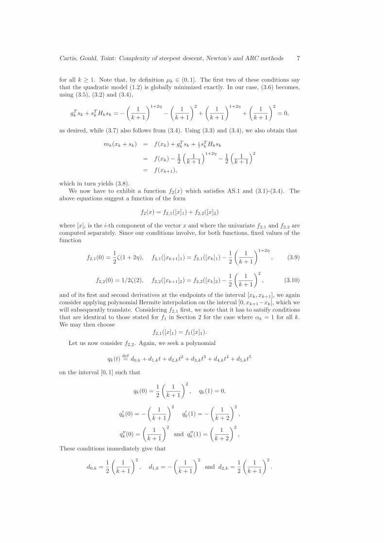
The resulting function is bounded below (by zero), continuously differentiable on IR (asthus satisfies AS.2) and twice continuously differentiable everywhere except at ζ(3/2),where both left and right second derivatives are infinite (it is therefore not Lipschitzcontinuous either). It also has a unique minimizer in ζ(3/2). The graph of this functionand its first three derivatives on the first 16 intervals are shown in Figure 3.4.

It is unclear whether an example with τ = η = 0 can be found without weakeningthe smoothness assumptions made at the start of this section, as we have just done.Interestingly, yet another example of Θ(ǫ−2) convergence for Newton’s method may beconstructed along the lines of the one just presented, by defining Hk, the Hessian at xk,to be

√k + 1 instead of k + 1. The minimum of the function f is then at infinity, but

continuous second derivatives are preserved although they remain unbounded.

4 How slow is slow?

Having shown an example where the performance of Newton’s method is arbitrarily closeto the worst case known for steepest descent, we now wish to comment on the degree ofpessimism of this bound.

Returning to multidimensional case, let us assume that (2.2) holds for some sequence ofiterates {xk} ⊂ IRn generated by Newton’s method on a twice continuously differentiable


0 0.5 1 1.5 2 2.50

0.1

0.2

0.3

0.4

0.5

0.6

0.7

0.8

0.9

0 0.5 1 1.5 2 2.5−1

−0.9

−0.8

−0.7

−0.6

−0.5

−0.4

−0.3

−0.2

−0.1

0

0 0.5 1 1.5 2 2.5−50

−40

−30

−20

−10

0

10

20

30

40

50

0 0.5 1 1.5 2 2.5−2

−1

0

1

2

3

4x 10

4


objective function from IRn into IR which is also bounded below and has uniformly boundedHessian. Assume also that Hk is positive definite for all k and that the unit step is taken atevery iteration of this process. Assume finally that the quadratic model (1.2) is minimizedaccurately enough to guarantee a model reduction at least as large as a fraction κ of thatobtained at the Cauchy point, which is defined as the solution of the (strictly convex)problem

mint≥0

mk(xk − tgk).

It is known (see Conn et al., 2000, Section 6.3.2, for instance) that the solution tCk of thislast problem and the associated model reduction satisfy

f(xk)−mk(xk − tCk gk) ≥ ‖gk‖42gT

k Hkgk.

Thus our assumption yields that

f(xk)−mk(xk + sk) ≥ κ‖gk‖42gT

k Hkgk≥ κ‖gk‖2

2‖Hk‖≥ κ

2κH‖gk‖2, (4.1)

where we used the Cauchy-Schwartz inequality to deduce the penultimate inequality andwhere κH is an upper bound on the Hessian norms. Because unit steps are taken, weobtain from (2.2) and (4.1) that

f(x0)− flow ≥ κ∞∑

k=0

f(xk)−mk(xk + sk) ≥ κ

2κH

∞∑

k=0

1

k + 1, (4.2)


where flow is a lower bound on f(x). But this last inequality is impossible because theharmonic series diverges. Hence we conclude that (2.2) cannot hold for our sequence ofiterates. Thus a gradient sequence satisfying (2.3) is essentially as close to (2.2) as possibleif the example is to be valid for all ǫ sufficiently small.

We may even pursue the analysis a little further. Let K denote the subset of theintegers such that (2.2) holds. Then (4.2) implies that

∑

k∈K

1

k + 1< +∞.

We then know from Behforooz (1995) that, in this case,

limℓ→∞

| K ∩ Nℓ |10ℓ − |K ∩ Nℓ |

= 0, (4.3)

where Nℓdef= {p ∈ IN | 0 ≤ p ≤ 10ℓ}. But

| K ∩ (Nℓ \ Nℓ−1) |10ℓ − 10ℓ−1

≤ 10| K ∩ Nℓ |9× 10ℓ

≤ 10

9

| K ∩ Nℓ |10ℓ − |K ∩ Nℓ |

and therefore, using (4.3),

limℓ→∞

| K ∩ (Nℓ \ Nℓ−1) || Nℓ \ Nℓ−1 |

= limℓ→∞

| K ∩ (Nℓ \ Nℓ−1) |10ℓ − 10ℓ−1

= 0.

Thus, if ℓ(k) is defined k such that k ∈ Nℓ(k) \ Nℓ(k)−1, we have that limk→∞ ℓ(k) = ∞and therefore that

limk→∞

Probk

[

‖gk‖ ≥ (k + 1)−2]

= limk→∞

Probk[ k + 1 ∈ K ]

= limk→∞

Probk[ k + 1 ∈ K ∩ (Nℓ(k) \ Nℓ(k)−1) ]

= 0

where Probk[·] is the probability with uniform density on {10ℓ(k)−1 + 1, . . . , 10ℓ(k)}. As aconsequence, the probability that the termination test (2.1) is satisfied for an arbitrary k

in the range [ 10ℓ(⌊ǫ−1/2⌋−1) + 1, 10ℓ(⌊ǫ−1/2⌋) ] tends to one when ǫ tends to zero.How do we interpret these results? What we have shown is that, under the conditions

stated before, the statement

there exists θ > 0 such that, for all k arbitrarily large, ||gk|| ≥ θ

(

1

k + 1

)2

is false. This is to say that

for all θ > 0 there exists k arbitrarily large such that ||gk|| < θ

(

1

k + 1

)2

.

In fact, we have proved that the proportion of “good” k’s for which this last inequalityholds (for a given θ) grows asymptotically. But it is important to notice that this laststatement doe not contradicts the worst-case bound of O(ǫ−2) mentioned above, which is

there exists θ > 0 such that, for all ǫ > 0 and k ≥ θ

ǫ2, ‖gk‖ ≤ ǫ.

Indeed, if ǫ is given, there is no guarantee that the particular k such that k = θ(k + 1)−2

belongs to the set of “good” k’s. As a consequence, we see that the worst-case analysis isincreasingly pessimistic for ǫ tending to zero.

We conclude this section by noting that the arguments developped for Newton’s methodalso turn out to apply for the steepest descent method, as it can also be shown for thiscase that

f(xk)−mk(xk − tCk gk) ≥ κSD‖gk‖2,for some κSD > 0 depending on the maximal curvature of the objective function (see, forinstance, Conn et al., 2000, Theorem 6.3.3 with ∆k sufficiently large, or Nesterov, 2004,relation (1.2.13) page 27). This inequality then replaces (4.1) in the above reasoning.


5 Less slow convergence for ARC

Now consider using the ARC algorithm for solving (1.1), using exact second-order informa-tion. As above, we would like to construct an example on which ARC converges at a ratewhich corresponds to its worst-case behaviour for general nonconvex objective functions,i.e. such that one has to perform O(ǫ−

3

2 ) iterations to ensure (2.1). In order to achievethis goal, a suitable condition is now to require that

‖gk‖ ≥(

1

k + 1

)2

3

.

An arbitrarily close approximation is again considered by requiring that, for any τ > 0,the ARC method needs O(ǫ−

3

2+τ ) iterations to achieve (2.1), which leads to the condition

that, for all k ≥ 0,

‖gk‖ =

(

1

k + 1

)2

3−2τ

. (5.1)

Our new objective is therefore to construct sequences {xk}, {gk}, {Hk}, {σk} and {fk}such that (5.1) holds and which may be generated by the ARC algorithm, together witha function f4(x) satisfying AS.1 such that (3.1) holds, which is bounded below and whoseHessian ∇xxf4(x) is Lipschitz continuous with global Lipschitz constant L ≥ 0.

Our example is now unidimensional and we define, for all k ≥ 0,

x0 = 0, xk+1 = xk +

(

1

k + 1

)1

3+η

, (5.2)

f4,0 =2

3ζ(1 + 3η), f4,k+1 = f4,k −

2

3

(

1

k + 1

)1+3η

, (5.3)

gk = −(

1

k + 1

)2

3+2η

, Hk = 0 and σk = 1, (5.4)

where now

η = η(τ)def=

1

2

(

2

3− 2τ− 2

3

)

=2τ

9− 6τ> 0.

Observe that (5.4) gives (5.1) by construction.Let us verify that, provided (3.1) holds, the sequences given by (5.2)–(5.4) may be

generated by the ARC algorithm, whose every iteration is very successful. Using (1.3),this amounts to verifying that

gTk sk + sT

kHksk + σk‖sk‖3 = 0, (5.5)

sTkHksk + σk‖sk‖3 ≥ 0, (5.6)

σk > 0, σk+1 ≤ σk (5.7)

andf4(xk + sk) = mk(xk + sk) (5.8)

for all k ≥ 1. Because the model is unidimensional, the first two of these conditions saysthat the cubic model is globally minimized exactly. Observe first that (5.7) immediatelyresults from (5.4). In our case, (5.5) becomes, using (5.2) and (5.4),

gTk sk + sT

kHksk + σk‖sk‖3 = −(

1

k + 1

)1+3η

+ 0 +

(

1

k + 1

)1+3η

= 0,


as desired, while inequality (5.6) also follows from (5.2) and (5.4). Using (5.3) and (5.4),we also obtain that

mk(xk + sk) = f4(xk) + gTk sk + 1

2sT

kHksk + 1

3σk‖sk‖3

= f4(xk)− 23

(

1k+1

)1+3η

= f4(xk+1),

which in turn yields (5.8).As was the case in the previous sections, the only remaining question is to exhibit

bounded below and twice continuously differentiable function f4(x) with a Lipschitz con-tinuous Hessian (in each segment [xk, xk+1]) satisfying conditions (5.2)-(5.4), and we mayonce more consider applying polynomial Hermite interpolation on the interval [0, xk+1 −xk]. Thus we are seeking a polynomial of the form (2.11) on the interval [0, sk] such that

pk(0) =2

3

(

1

k + 1

)1+3η

, pk(sk) = 0 (5.9)

p′k(0) = −(

1

k + 1

)2

3+2η

, p′k(sk) = −(

1

k + 2

)2

3+2η

and p′′k(0) = p′′k(sk) = 0. (5.10)

These conditions immediately give that

c0,k =2

3

(

1

k + 1

)1+3η

, c1,k = −(

1

k + 1

)2

3+2η

and c2,k = 0.

In this case, the remaining interpolation conditions may be written in the form

s3k s4k s5k3s2k 4s3k 5s4k6sk 12s2k 20s3k

c3,k

c4,k

c5,k

=

pk(sk)− pk(0)− p′k(0)sk

p′k(sk)− p′k(0)0

,

whose solution is now given by

c3,k

c4,k

c5,k

=

103 − 4φk

1sk

[−5 + 7φk]

1s2

k

[2− 3φk]

(5.11)

with

φkdef= (k + 1)µ

[(

1

k + 1

)µ

−(

1

k + 2

)µ]

where µdef=

2

3+ 2η.

The definition of φk implies that φk ∈ (0, 1) for all k ≥ 0, and hence, using (5.11), that

|p′′′(t)| = 6c3,k + 24c4,kt+ 60c5,kt2

≤ 6c3,k + 24c4,ksk + 60c5,ks2k

≤ 6× 103 + 24× 13 + 60× 2

= 452

(5.12)

for all k ≥ 0 and all t ∈ [0, sk], and f has Lipschitz continuous second derivatives along thepath of iterates, which is IR+. The desired objective function for our final counterexampleis then recursively defined on the nonnegative reals(2) by

f4(x) = pk(x− xk) + f4(xk+1) for x∈[xk, xk+1] and k ≥ 0,

(2)Again, it can be easily smoothly extended to the negative reals while maintaining its boundednessand the Lipschitz continuity of its second derivatives.


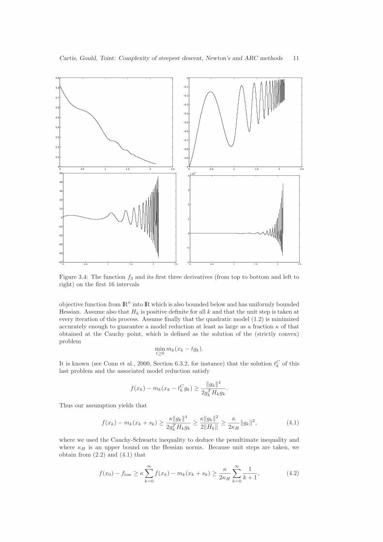
and clearly satisfies AS.1. The graph of this function and its first three derivatives aregiven on the first 16 intervals and for η = 10−4 by Figure 5.5. This figure confirms theproperties of the function f4(x), namely that it is twice continuous differentiable andhas uniformly bounded third derivative (in Figure 5.5, the maximum is achieved on eachinterval by the first point in the interval, where (5.11) and (5.12) imply that |p′′′(0)| ≤ 20).Thus its second derivative is globally Lipschitz continuous with constant L ≤ 452 (L = 20for the function plotted). As in our first example, the figure reveals the nonconvexityand monotonically decreasing nature of f(x). The fact that f(x) is bounded below byzero finally results from (5.3) and the definition of the Riemann ζ function (note thatζ(1.0003) ≈ 33333.9).

0 1 2 3 4 5 6 7 8 92.222

2.222

2.2221

2.2222

2.2222

2.2222

2.2223x 10

4

0 1 2 3 4 5 6 7 8 9−1

−0.9

−0.8

−0.7

−0.6

−0.5

−0.4

−0.3

−0.2

−0.1

0

0 1 2 3 4 5 6 7 8 9−1

−0.5

0

0.5

1

1.5

0 1 2 3 4 5 6 7 8 9−10

−5

0

5

10

15

20


6 Conclusions

We now summarize the result obtained in this paper. Considering the steepest methodfirst and assuming Lipzschitz continuity of the objective function’s gradient along thepath of iterates, we have, for any τ > 0, exhibited valid examples for which this algorithmproduces a sequence of slowly converging gradients. This in turn implies that, for anyǫ ∈ (0, 1) at least

⌊

1

ǫ2−τ

⌋

iterations and function evaluations are necessary for this algorithm to produce an iteratexk such that ‖gk‖ ≤ ǫ. This lower bound is arbitrarily close to the upper bound ofO(ǫ−2) known for this algorithm. Other examples have also been constructed showing


that the same complexity can be achieved by Newton’s method for twice continuouslydifferentiable functions whose Hessian is Lipschitz continuous on the path defined by theiterates, thereby proving that Newton’s method may be as (in)efficient as the steepestdescent method (in its worst-case). The fact that (3.8) and (5.8) hold ensures that ourconclusions are also valid if the standard Newton’s method is embedded in a trust-regionglobalization framework (see Conn et al., 2000 for an extensive coverage of such methods),since it guarantees that every iteration is very successful in that case, and that the initialtrust-region may then be chosen large enough to be irrelevant. The conclusions alsoapply if a linesearch globalization is used (see Dennis and Schnabel, 1983, or Nocedaland Wright, 1999), because the unit step is then acceptable at every iteration, or in thefilter context, because the gradient is monotonically converging to zero. We have alsoprovided an example where Newton’s method requires exactly 1/ǫ2 iterations to producean iterate xk such that ‖gk−1‖ ≤ ǫ, but had to give up boundedness of second derivativesto obtain this sharper bound. In addition, we have provided some analysis in an attemptto quantitfy how pessimistic the obtained worst-case bounds can be.

We have then extended the methodology to cover the Adaptive Regularization with Cu-bics (ARC) algorithm, which can be viewed as a regularized version of Newton’s method.For any τ > 0, we have exhibited a valid example for which the ARC algorithm producesa sequence of gradients satisfying (5.1). This equality yields that, for any ǫ ∈ (0, 1) atleast

⌊

1

ǫ3

2−τ

⌋

iterations and function evaluations are necessary for this algorithm to produce an iteratexk such that ‖gk‖ ≤ ǫ. This lower bound is arbitrarily close to the upper bound ofO(ǫ−3/2)thereby proving that this last bound is sharp.

In our examples for the Newton’s and ARC methods, exact global model minimizationis carried out, covering the “exact” variants of these algorithms. But the conditions used((3.6)-(3.7) and (5.5)-(5.6)) only require this exact minimization to occur along the stepsk, which makes the conclusions presented in this paper applicable if one prefers usingapproximate minimization where the global model minimum is only sought in subspaces,as in the case for truncated conjugate-gradients (see Steihaug, 1983, and Toint, 1981),GLTR (Gould, Lucidi, Roma and Toint, 1999, LSTR and LSRT (Cartis, Gould and Toint,2009c), or for other subspace methods (Ni and Yuan, 1997, Hager, 2001, Erway, Gilland Griffin, 2009). This is however less surprising, as one could expect approximateminimization to deteriorate the global effiency of the minimization algorithm.

We have not been able to show that the steepest descent method may take at leastO(ǫ−2) evaluations to achieve a gradient accuracy of ǫ on functions with Lipschitz con-tinuous second derivatives, thereby not exluding the (unlikely) possibility that steepestdescent could be better than Newton’s method on sufficiently smooth functions.

Our result that the ARC method is the best second-order algorithm available so far(from the worst-case complexity point of view) suggests further research directions beyondthat of settling the open question mentoned in the previous paragraph. Is the associatedcomplexity bound in O(ǫ−3/2) the best that can be achieved by any second-order methodfor general nonconvex objective functions? And how best to characterize the complexityof an unconstrained minimization problem? These interesting issues remain challenging.

Acknowledgements

The work of the second author has been supported by the EPSRC grant EP/E053351/1. The third author

gratefully acknowledges the support of EPSRC grant EP/G038643/1, and of the ADTAO project funded

by the “Sciences et Technologies pour l’Aeronautique et l’Espace (STAE)” Fundation (Toulouse, France)

within the “Reseau Thematique de Recherche Avancee (RTRA)”.


References

H. Behforooz. Thinning out the harmonic series. Mathematics Mag-azine, 68(4), 289–293, 1995. As cited on http://www.cut-the-knot.org/arithmetic/algebra/HarmonicSeries.shtml.

C. Cartis, N. I. M. Gould, and Ph. L. Toint. Adaptive cubic overestimation methodsfor unconstrained optimization. Part II: worst-case iteration complexity. TechnicalReport 07/05, Department of Mathematics, FUNDP - University of Namur, Namur,Belgium, 2007.

C. Cartis, N. I. M. Gould, and Ph. L. Toint. Adaptive cubic overestimation methods forunconstrained optimization. Part I: motivation, convergence and numerical results.Mathematical Programming, Series A, 2009a. DOI: 10.1007/s10107-009-0286-5, 51pages.

C. Cartis, N. I. M. Gould, and Ph. L. Toint. Efficiency of adaptive cubic regularisationmethods on convex problems. Technical Report (in preparation), Department ofMathematics, FUNDP - University of Namur, Namur, Belgium, 2009b.

C. Cartis, N. I. M. Gould, and Ph. L. Toint. Trust-region and other regularisation of linearleast-squares problems. BIT, 49(1), 21–53, 2009c.

A. R. Conn, N. I. M. Gould, and Ph. L. Toint. Trust-Region Methods. Number 01 in‘MPS-SIAM Series on Optimization’. SIAM, Philadelphia, USA, 2000.

J. E. Dennis and R. B. Schnabel. Numerical Methods for Unconstrained Optimization andNonlinear Equations. Prentice-Hall, Englewood Cliffs, NJ, USA, 1983. Reprinted asClassics in Applied Mathematics 16, SIAM, Philadelphia, USA, 1996.

J. B. Erway, P. E. Gill, and J. D. Griffin. Iterative methods for finding a trust-region step.SIAM Journal on Optimization, 20(2), 1110–1131, 2009.

R. Fletcher. Practical Methods of Optimization. J. Wiley and Sons, Chichester, England,second edn, 1987.

N. I. M. Gould, S. Lucidi, M. Roma, and Ph. L. Toint. Solving the trust-region subproblemusing the Lanczos method. SIAM Journal on Optimization, 9(2), 504–525, 1999.

N. I. M. Gould, C. Sainvitu, and Ph. L. Toint. A filter-trust-region method for uncon-strained optimization. SIAM Journal on Optimization, 16(2), 341–357, 2005.

S. Gratton, A. Sartenaer, and Ph. L. Toint. Recursive trust-region methods for multiscalenonlinear optimization. SIAM Journal on Optimization, 19(1), 414–444, 2008.

A. Griewank. The modification of Newton’s method for unconstrained optimization bybounding cubic terms. Technical Report NA/12, Department of Applied Mathemat-ics and Theoretical Physics, University of Cambridge, Cambridge, United Kingdom,1981.

W. W. Hager. Minimizing a quadratic over a sphere. SIAM Journal on Optimization,12(1), 188–208, 2001.

Yu. Nesterov. Introductory Lectures on Convex Optimization. Applied Optimization.Kluwer Academic Publishers, Dordrecht, The Netherlands, 2004.

Yu. Nesterov. Accelerating the cubic regularization of Newton’s method on convex prob-lems. Mathematical Programming, Series A, 112(1), 159–181, 2008.

Yu. Nesterov and B. T. Polyak. Cubic regularization of Newton method and its globalperformance. Mathematical Programming, 108(1), 177–205, 2006.


Q. Ni and Y. Yuan. A subspace limited memory quasi-Newton algorithm for large-scale nonlinear bound constrained optimization. Mathematics of Computation,66(220), 1509–1520, 1997.

J. Nocedal and S. J. Wright. Numerical Optimization. Series in Operations Research.Springer Verlag, Heidelberg, Berlin, New York, 1999.

R. Polyak. Regularized Newton method for unconstrained convex optimization. Mathe-matical Programming, Series A, 120(1), 125–145, 2009.

T. Steihaug. The conjugate gradient method and trust regions in large scale optimization.SIAM Journal on Numerical Analysis, 20(3), 626–637, 1983.

Ph. L. Toint. Towards an efficient sparsity exploiting Newton method for minimization. inI. S. Duff, ed., ‘Sparse Matrices and Their Uses’, pp. 57–88, London, 1981. AcademicPress.

K. Ueda. Regularized Newton Method without Line Search for Unconstrained Optimization.PhD thesis, Department of Applied Mathematics and Physics, Graduate School ofInformatics, Kyoto University, Kyoto, Japan, 2009.

K. Ueda and N. Yamashita. Convergence properties of the regularized Newton methodfor the unconstrained nonconvex optimization. Technical Report 2008-015, Depart-ment of Applied Mathematics and Physics, Graduate School of Informatics, KyotoUniversity, Kyoto, Japan, 2008.

K. Ueda and N. Yamashita. Regularized Newton method without line search for uncon-strained optimization. Technical Report 2009-007, Department of Applied Mathe-matics and Physics, Graduate School of Informatics, Kyoto University, Kyoto, Japan,2009.

M. Weiser, P. Deuflhard, and B. Erdmann. Affine conjugate adaptive Newton methodsfor nonlinear elastomechanics. Optimization Methods and Software, 22(3), 413–431,2007.

on the complexity of steepest descent, newton’s and ... · on the complexity of steepest descent,...

Documents