Uppsala University

Department of Statistics

On Statistical Arbitrage:

Cointegration and Vector Error-Correction in the Energy Sector

BY OSCAR NILSSON* AND EMMANUEL LATIM OKUMU†

SUPERVISOR: LARS FORSBERG

Spring 2014

Abstract

* Oscar.nilsson.4839@student.uu.se † Emmanuel.okumu.9117@student.uu.se

This paper provides methods to select pairs potentially profitable within the

frame of statistical arbitrage. We employ a cointegration approach on

pairwise combinations of five large energy companies listed on the New

York Stock Exchange for the period 27th

September 2012 to 22nd

April

2014. We find one cointegrated pair, for which we further investigate both

short and long run dynamics. A vector-error correction model is

constructed, supporting a long run relationship between the two stocks,

which is also supported by the mean-reverting characteristic of a stationary

linear combination of the stocks. Impulse response functions and variance

decomposition are also studied to further describe the interrelation of the

stocks, supporting a unidirectional causality between the stocks.

Keywords: Mean-reversion, VAR, VECM, impulse response, cointegration

We would like to thank our supervisor, Lars Forsberg, for his support and advice

throughout this work.

2

Table of contents

Introduction ............................................................................................................................. 3

Theory....................................................................................................................................... 5

Stationarity and Unit root processes ...................................................................................... 5

Cointegration ......................................................................................................................... 6

Multivariate systems .............................................................................................................. 8

Arbitrage Pricing Theory ..................................................................................................... 12

Methodology ........................................................................................................................... 14

Augmented Dickey-Fuller ................................................................................................... 14

The Engle & Granger approach ........................................................................................... 14

Johansen’s test ..................................................................................................................... 15

Impulse Response ................................................................................................................ 16

Variance Decomposition ..................................................................................................... 19

Data ..................................................................................................................................... 20

Results..................................................................................................................................... 22

Vector Error-Correction ...................................................................................................... 24

Impulse Response ................................................................................................................ 25

Variance Decomposition ..................................................................................................... 27

Conclusions ............................................................................................................................ 28

Bibliography........................................................................................................................... 29

Appendix A ............................................................................................................................ 31

3

Introduction

In the early 80’s, Clive Granger (1981) introduced the concept of cointegration. The basic

idea is that two variables that each are integrated of some order may form a linear

combination that is integrated of a lower order. In its simplest form, an example is the case

where two variables each follow a random walk, but a linear combination of the two is

stationary. The stationarity of the combination implies that the variables conform to a long-

run equilibrium, and that deviations from the equilibrium are merely temporary. In economics,

cointegration is commonly used to describe the relationship between related variables such as

short and long interest rates, income and consumption or in the theory of Purchasing Power

Parity. This aspect of long-run equilibrium has also gained attention in the financial industry,

and the term statistical arbitrage refers to the profitable potential of trading a cointegrated pair

of stocks. Consider two securities that are cointegrated and therefore expected to move

together in the long run. If any of the securities were to deviate from this co-movement, it

would suggest a temporary mispricing. We might not know which security that is actually

mispriced, but we know that their relative prices are incorrect. One could then take a short

position (sell) in the relatively overvalued stock, and a long position (buy) in the relatively

undervalued stock. When the securities return to their long-run equilibrium, the positions are

unwinded to a profit. When employing this strategy, it is desirable to enter the positions when

the deviation from the equilibrium is at its largest. This is of course unknown beforehand,

however, the larger the relative mispricing is when the positions are taken, the larger the

potential profit.

Do, Faff and Hamza (2006) examine three pairs of stocks based on industry similarity,

seeking to find a pair for which a long-short positioning would be profitable when the pair

diverges from its long-run relationship. Because of the proprietary nature of the subject,

literature is rather limited, and they therefore present several techniques that may be applied

to the study. Through their analysis they find cointegrated stocks, but because of an

increasing divergence in the relationship, the pairs would be considered to risky to take action

on. Gatev et al. (2006) investigates a large sample of stocks for the period of 1962 – 2002.

Employing a minimum distance method when observing normalized prices of stocks that

seem to move together, they find that pairs trading is a profitable strategy. The idea of pairs

trading can be applied to other assets than stocks, Jacobsen (2008) examines the relationship

between two exchange-traded funds (ETF) with large overlap in coverage. Using intraday

data (minute by minute) for a period of 3 months and taking transaction costs into account he

finds that the strategy is very profitable compared to a buy & hold strategy for the two assets.

To assess this relationship he employs the Johansen’s test and the Engle and Granger

4

approach, emphasizing the importance of the error-correction model in order to study the

short-run and long-run dynamics. The error-correction representation is also adopted by Kniff

and Pynnönen (1999) when estimating a VAR for the cross-dependency of eleven different

stock market indices. Finding that the Swedish index and the Norwegian index are

cointegrated they construct a vector error-correction model to further analyse the relationship.

This paper will aim to describe a methodology of how to find a cointegrated pair of stocks

that could be profitable to trade. The search for cointegrated pairs is commonly encouraged to

take place between assets that are related by industry and other characteristics that both can

support any fundamental relationship and that the cointegration remains significant out-of-

sample (Vidyamurthy, 2004). In this paper, five different energy companies listed on the New

York Stock Exchange are examined. Data are collected for the period 27 September 2012 to

22 April 2014, and the properties of the time series are inspected. We then test the ten

possible pairwise combinations for cointegration by the Johansen’s test and the Engle and

Granger approach. Of the ten pairs, we find one to be cointegrated over the entire sample

period. We investigate the cointegrating relationship by constructing a Vector Error-

Correction Model and conduct further analysis of the relationship through impulse response

functions and variance decomposition.

The rest of the paper is organized as follows. In section 2 we describe the theoretical

framework of cointegration and also explain the error-correction representation. The

following section presents the Johansen’s test and the Engle & Granger approach, which both

will be applied in study. Impulse response functions and variance decomposition are covered

and a presentation of the data employed in the study is also given. Section 4 summarizes our

results and our conclusions are presented in Section 5.

5

Theory

Stationarity and Unit root processes

A key concept underlying the idea behind cointegration is stationarity. Stationarity refers to a

time series that exhibits certain characteristics that are of great importance to econometric

analysis. Distinction is made between strong stationarity and weak stationarity. The latter,

also referred to as covariance stationarity, will be of interest throughout the paper, given that

strong stationarity is difficult to assess. For a time series to be covariance stationary it

requires the following characteristics:

( ) ( )

( ) ( )

( )( ) ( )( ) .

The first condition implies a constant mean over time, this ensures that deviations from the

mean are temporary and the series is expected to revert back to the long run mean. The

second condition concerns the second moment, the variance, which should be finite and

constant over time. Lastly, the covariance between different variables is only dependent on

the lag length, not on time. A time series generated from a simple AR(1) process,

, is stationary for values of | | . The model fulfils the three conditions with an

expected mean of zero, a variance of ( ) and the covariance (

( )). To

extend the above example, the general ARMA(p, q) is given by,

∑

∑

using lag operators,

( ) (

)

( ) ( )

Since the ARMA(p, q) is made up of an AR(p) and a MA(q), and the MA(q) is always

stationary, the stationarity of the model is dependent on the AR(p)-part. If all the roots of the

characteristic equation ( ) are outside the unit circle, then the model is stationary. The

ARMA(p, q) is a case of the ARIMA(p, d, q), where I(d), the order of integration, is zero. A

time series that is integrated, but stationary when taking the difference d times, is integrated

6

of order d. To illustrate the case of an integrated series we can return to the AR(1) model but

we let . Then the model is simply , a random walk, and it is no longer

stationary as it contains a unit root. The series will have an infinite memory as shocks to the

series will have permanent effect, and the variance will grow to infinity as time goes to

infinity. (Asteriou & Hall, 2011) Differencing the series once gives , simply

stationary white noise. In economics it is not unusual to study series that contain unit root,

therefore it is common practice to difference the series until stationarity is obtained before

conducting regression analysis. If this is ignored, the researcher will likely obtain spurious

results, meaning they have no actual meaning at all. It is however not guaranteed that all

integrated series can be differenced to become stationary. Stationarity and order of integration

play an important role in the concept of cointegration, which will be discussed next.

Cointegration

If conducting regression analysis using integrated series, the researcher runs the risk of

obtaining spurious results and integrated residual series that invalidates the estimates. The

concept of cointegration was introduced by Granger (1981), the very special case when a

linear combination of series that are integrated of the same order, is integrated by a lower

order. That is, if two series { } are ( ), but a linear combination of the series is ( ),

where , then the series are cointegrated, presented as { } ( ) . More

generally, let be a ( ) vector of series and that each series is ( ). If

there exists a ( ) vector that gives ( ), we have that ( ). When the

series are cointegrated, the analysis of their relationship is not spurious, and no differencing

of the variables to reach stationarity is needed before examining their relationship. (Asteriou

& Hall, 2011)

Consider the case where { } and { } both are ( ), but a vector { } exists that give

that is ( ). The series are then cointegrated, resulting in a stationary linear

combination. This implies a long-run equilibrium around which the variables are allowed to

fluctuate. The shocks that may affect the equilibrium are merely temporary, since the

stationarity ensures mean-reversion that restores the long-run equilibrium. Given that our

variables are cointegrated it is of interest to study the long-run relation of the variables. The

error-correction model (ECM) is a convenient reparametrization of the autoregressive

distributed lag model (ADL). The ECM allows us to study both short-run and long-run effects

and its popularity is extensive in applied time series econometrics. The ECM is presented in

the Granger Representation Theorem by Engle and Granger (1987) for cointegrated series. A

general reparametrization of the ADL to the ECM is given below and then a corresponding

7

approach for the multivariate case. The ADL model for and with and lags

respectively is given in Equation 1 (Asteriou & Hall, 2011).

∑ ∑

1

In the long run, for two cointegrated variables, the relationship can be expressed as,

2

assuming that and rearranging the terms,

∑

∑

∑ 3

4

Let

and

, then can be expressed as conditional on

a constant value of in time as in Equation 5. Equation 6 now illustrates the error that

occurs when deviates from the long-run .

5

6

To move further towards the ECM, Equation 1 is reparametrized to Equation 7 below,

∑ ∑

7

where ∑ and ( ∑ ) . Let the long-run parameter and

.

This will lead to Equation 9 by,

∑ ∑ (

)

8

∑ ∑ ( ̂ ̂ )

9

8

∑ ∑ ̂

10

At last, Equation 10 states the ECM in its final representation and we reach the essence of the

model, the parameter . This error-correction coefficient is interpreted as the speed at which

the model corrects for the error, i.e. the deviation from the long-run equilibrium, which might

have occurred in the previous period. In a cointegrated relationship, it should also be noted

that Granger causality must run in at least one direction. Granger causality refers to when a

variable can be more accurately predicted if it is not only explained by its own lagged terms,

but also by the other variables lagged terms. In the ECM the Granger causality of on can

therefore be detected either by a significant coefficient for the lagged terms of or by the

coefficient for the lagged error-correction part, which contains the lagged term of (Asteriou

and Hall, 2011)

Multivariate systems

We will now expand the ideas from the previous example by presenting how we can model

multiple time series in a system of equations. Sims (1980) stressed the reasoning of

representing multiple economic variables in a dynamic system noting that there is interaction

among a set of variables describing the economy, where the dependent variable might also be

an important explanatory variable of the initial ‘explanatory variable’. Another view of this is

given by Asteriou & Hall (2011), they express that if we do not know if a variable is

endogenous or exogenous each variable has to be treated symmetrically. In other words we

need to treat the variables as both exogenous and endogenous variables. Since we will try to

analyse a set of sequences simultaneously that we hypothesize has some interaction between

them, it is reasonable to develop a system of equations in which this interaction is considered.

A widely popular class of these multivariate equations is the vector autoregressive model

(VAR). The VAR is a natural extension of the univariate autoregressive model to dynamic

multivariate time series. The model has been proven to be superior to its univariate equivalent

for modeling multiple economic time series whilst capturing the linear interdependencies. As

mentioned earlier, we might have a long run relationship between two sequences by a

cointegrated relationship. The multivariate equivalent of the ECM is naturally called a Vector

Error-Correction Model (VECM). The VECM allows long-run components of variables to

submit to equilibrium constraints while short-run components have a flexible dynamic

specification in a multivariate setting. Below we introduce the ideas underlying these

9

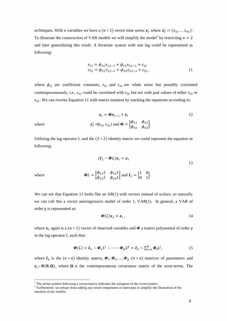
techniques. With n variables we have a ( ) vector time series where ( )*.

To illustrate the construction of VAR models we will simplify the model† by restricting

and later generalizing this result. A bivariate system with one lag could be represented as

following:

11

where are coefficient constants, and are white noise but possibly correlated

contemporaneously, i.e., could be correlated with but not with past values of either or

. We can rewrite Equation 11 with matrix notation by stacking the equations according to:

12

where =( ) and [

].

Utilizing the lag operator L and the ( ) identity matrix we could represent the equation as

following:

( ) 13

where [

] and [

]

We can see that Equation 12 looks like an AR(1) with vectors instead of scalars, so naturally

we can call this a vector autoregressive model of order 1, VAR(1). In general, a VAR of

order p is represented as:

( ) 14

where again is a ( ) vector of observed variables and a matrix polynomial of order p

in the lag operator L such that:

( )

∑

15

where is the ( ) identity matrix, ( ) matrices of parameters and

( ) , where is the contemporaneous covariance matrix of the error-terms. The

* The prime symbol following a vector/matrix indicates the transpose of the vector/matrix. † Furthermore, we refrain from adding any trend components or intercepts to simplify the illustration of the

intuition of the models.

10

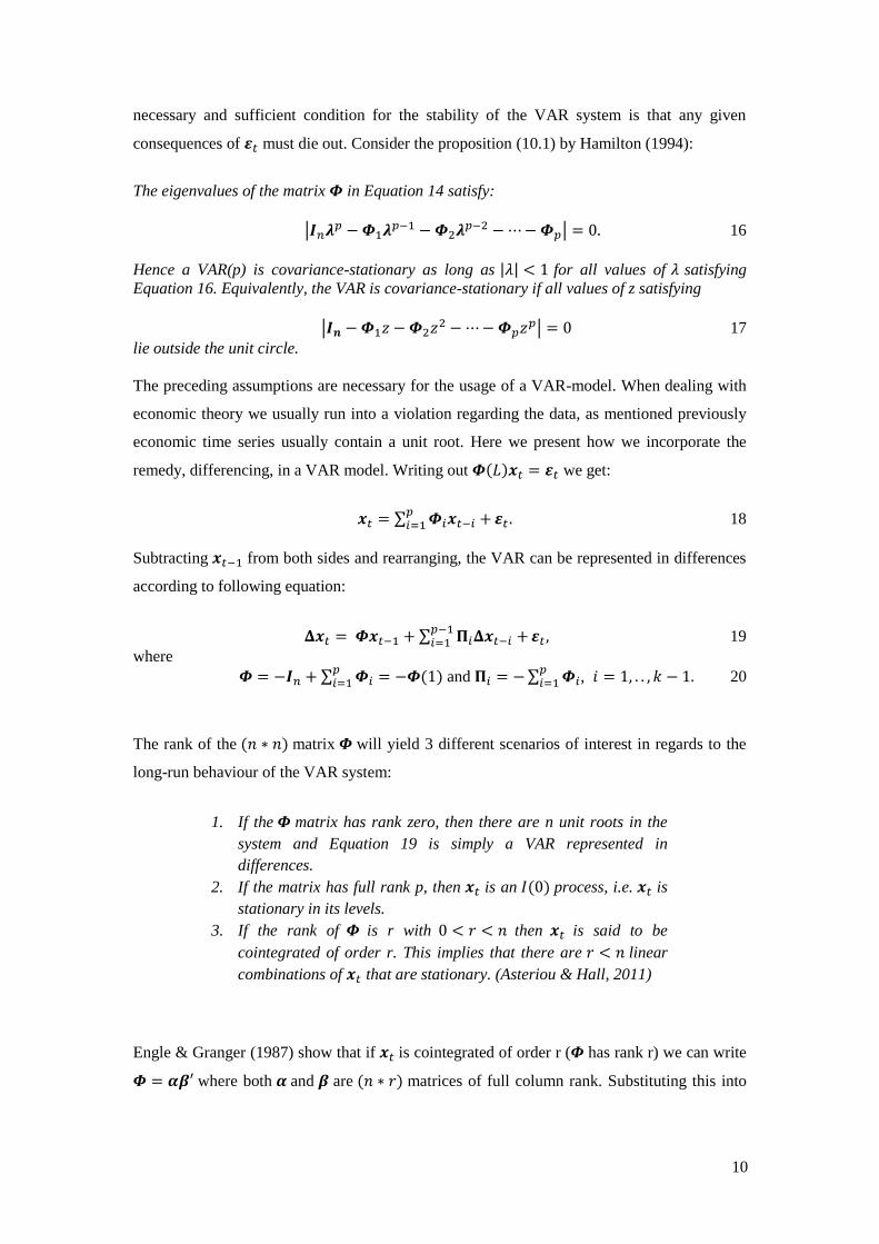
necessary and sufficient condition for the stability of the VAR system is that any given

consequences of must die out. Consider the proposition (10.1) by Hamilton (1994):

The eigenvalues of the matrix in Equation 14 satisfy:

|

| 16

Hence a VAR(p) is covariance-stationary as long as | | for all values of satisfying

Equation 16. Equivalently, the VAR is covariance-stationary if all values of z satisfying

|

| 17

lie outside the unit circle.

The preceding assumptions are necessary for the usage of a VAR-model. When dealing with

economic theory we usually run into a violation regarding the data, as mentioned previously

economic time series usually contain a unit root. Here we present how we incorporate the

remedy, differencing, in a VAR model. Writing out ( ) we get:

∑ 18

Subtracting from both sides and rearranging, the VAR can be represented in differences

according to following equation:

∑ 19

where

∑ ( ) and ∑

, 20

The rank of the ( ) matrix will yield 3 different scenarios of interest in regards to the

long-run behaviour of the VAR system:

1. If the matrix has rank zero, then there are n unit roots in the

system and Equation 19 is simply a VAR represented in

differences.

2. If the matrix has full rank p, then is an ( ) process, i.e. is

stationary in its levels.

3. If the rank of is r with then is said to be

cointegrated of order r. This implies that there are linear

combinations of that are stationary. (Asteriou & Hall, 2011)

Engle & Granger (1987) show that if is cointegrated of order r ( has rank r) we can write

where both and are ( ) matrices of full column rank. Substituting this into

11

the VAR in differences (Eq.19) allows us to write the VAR as the following vector error-

correction model (VECM):

∑ 21

where contains the r cointegrating vectors and are the r stationary linear

combinations of . Norman Morin of the US Federal Reserve Board offers some intuitive

interpretations of the variables. The matrix contains the r equilibrium relationships among

the variables. For these relationships, we can interpret the difference between the observed

values of and their expected values as measures of disequilibrium from the r different

long-run relationships. The matrix measures how quickly reacts to the deviation from

the equilibrium implied by (Morin, 2006).

To further explain the error-correction component in Equation 21, , we will restrict

r=2 cointegrating vectors and can then show that:

[

] [

] [

]

and thereby we have that:

[

]

[ ∑

∑

]

[ ∑

∑

∑

∑

]

These preceding considerations lead to the foundation of a model useable for the study of

pairs of variables. Since we are studying two cointegrated time series, we will now illustrate a

bivariate system. Hamilton (1994) lets (where is a stationary ( ) vector) and

shows that the first row of Equation 21 takes the following form:

( )

( ) . 22

( )

( )

( )

( )

12

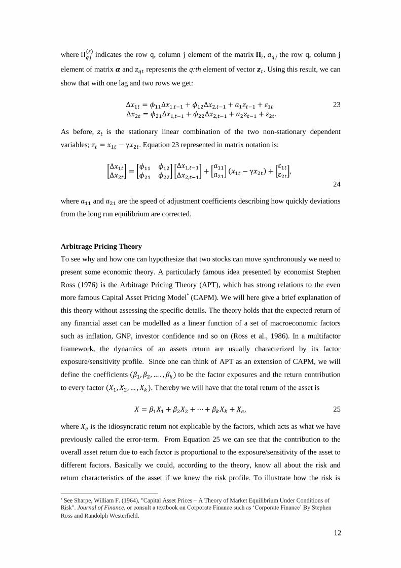
where ( )

indicates the row q, column j element of the matrix , the row q, column j

element of matrix and represents the q:th element of vector . Using this result, we can

show that with one lag and two rows we get:

23

As before, is the stationary linear combination of the two non-stationary dependent

variables; . Equation 23 represented in matrix notation is:

[

] [

] [

] [

] ( ) [

]

24

where and are the speed of adjustment coefficients describing how quickly deviations

from the long run equilibrium are corrected.

Arbitrage Pricing Theory

To see why and how one can hypothesize that two stocks can move synchronously we need to

present some economic theory. A particularly famous idea presented by economist Stephen

Ross (1976) is the Arbitrage Pricing Theory (APT), which has strong relations to the even

more famous Capital Asset Pricing Model* (CAPM). We will here give a brief explanation of

this theory without assessing the specific details. The theory holds that the expected return of

any financial asset can be modelled as a linear function of a set of macroeconomic factors

such as inflation, GNP, investor confidence and so on (Ross et al., 1986). In a multifactor

framework, the dynamics of an assets return are usually characterized by its factor

exposure/sensitivity profile. Since one can think of APT as an extension of CAPM, we will

define the coefficients ( ) to be the factor exposures and the return contribution

to every factor ( ). Thereby we will have that the total return of the asset is

25

where is the idiosyncratic return not explicable by the factors, which acts as what we have

previously called the error-term. From Equation 25 we can see that the contribution to the

overall asset return due to each factor is proportional to the exposure/sensitivity of the asset to

different factors. Basically we could, according to the theory, know all about the risk and

return characteristics of the asset if we knew the risk profile. To illustrate how the risk is

* See Sharpe, William F. (1964), "Capital Asset Prices – A Theory of Market Equilibrium Under Conditions of

Risk". Journal of Finance, or consult a textbook on Corporate Finance such as ‘Corporate Finance’ By Stephen

Ross and Randolph Westerfield.

13

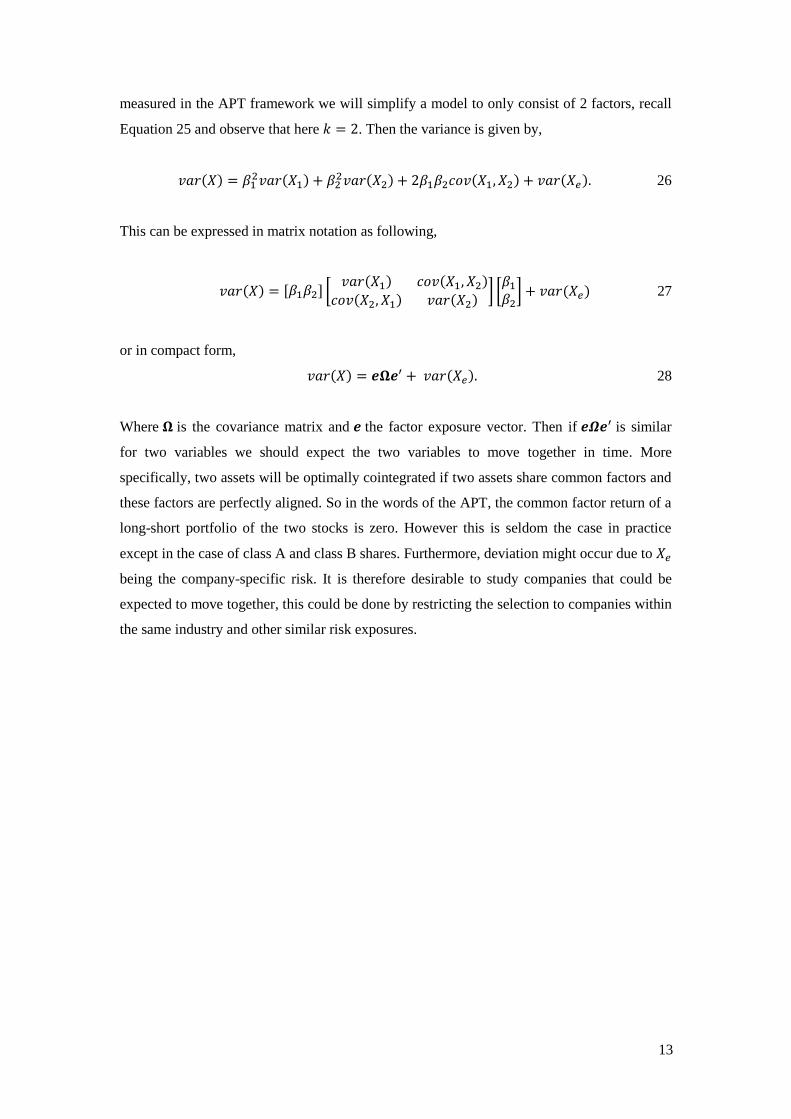
measured in the APT framework we will simplify a model to only consist of 2 factors, recall

Equation 25 and observe that here . Then the variance is given by,

( ) ( )

( ) ( ) ( ) 26

This can be expressed in matrix notation as following,

( ) [ ] [ ( ) ( )

( ) ( )] [

] ( ) 27

or in compact form,

( ) ( ) 28

Where is the covariance matrix and the factor exposure vector. Then if is similar

for two variables we should expect the two variables to move together in time. More

specifically, two assets will be optimally cointegrated if two assets share common factors and

these factors are perfectly aligned. So in the words of the APT, the common factor return of a

long-short portfolio of the two stocks is zero. However this is seldom the case in practice

except in the case of class A and class B shares. Furthermore, deviation might occur due to

being the company-specific risk. It is therefore desirable to study companies that could be

expected to move together, this could be done by restricting the selection to companies within

the same industry and other similar risk exposures.

14

Methodology

Augmented Dickey-Fuller

In 1979, Dickey and Fuller developed a test assessing the presence of a unit root in the series.

The Dickey-Fuller test starts with Equation 29,

( ) 29

where is white noise, and states the null hypothesis as ( ) and ( )

, which is tested through an ordinary t-test. The test statistic is however not evaluated

through the conventional t-values, it requires specific critical values originally developed by

Dickey and Fuller. See MacKinnon (1991) for full specification of the critical values. The test

is also able to account for an intercept and linear trend. Accepting the null implies that the

series contains a unit root and is therefore not stationary. The test was later extended to

include number of lags in the model given the likelihood that the term in Equation 29 is

not white noise. This extended version is the Augmented Dicker-Fuller test and the

corresponding equations when accounting for several lags in the model are:

∑ 30

∑ 31

∑ 32

As for the simple case the test can account for a constant and linear trend. Equation 31 takes

into account an intercept through the constant term , whereas Equation 32 accounts for both

the intercept as well as for a linear trend by the term (Asteriou & Hall, 2011).

The Engle & Granger approach

Before the development of the Johansen’s test, a way of assessing a potential cointegration

relationship had already been proposed by Engle & Granger (1987). The method is intuitive

and simple to perform, but has been criticized on some grounds. The Engle & Granger (EG)

approach is able to detect one cointegrating relationship between variables, in contrast to the

Johansen’s test, which is able to detect more than one, i.e., several cointegrating vectors. If

two variables are integrated of the same order, the simple regression is

15

constructed. If the variables really are cointegrated, the estimated ̂ from the OLS will

converge very quickly. The estimates for the error term, ̂ , are then tested for order of

integration by the ADF test. If the residuals are integrated of a lower order than the variables

themselves, we conclude that the variables are cointegrated and we proceed by estimating an

ECM. Given that the procedure involves two estimations before we reach a conclusion, the

EG approach is distorted by the fact than any errors from the first estimation of the residuals

are carried along to the second estimation where the residuals are tested for the order of

integration. Another obvious critique towards the EG approach is that only one cointegrating

relationship can be assessed, although there might be more than one cointegrating vector

when investigating more than two variables. Furthermore, the question arises for which

variable to place as the dependent variable. Asymptotically, the results will be equivalent, but

for samples that are not large enough it might give contradicting results. (Asteriou & Hall,

2011) In our analysis we will apply the Johansen’s method, crosschecking our finding by the

EG-approach.

Johansen’s test

In a VAR system where cointegrating relationships exists we found in the previous section

that the ( ) matrix can be decomposed into where is a ( ) matrix and is a

( ) matrix. From this decomposition it is possible to obtain important information about

the long-run relationship between the cointegrated series, the matrix contains the

coefficients for the cointegrating vectors and the matrix will give the coefficients for the

speed of adjustment. There can exist ( ) cointegrating relationships between variables,

and the Johansen’s test allows for the detection of more than one cointegrating relationship in

contrast to the Engle & Granger approach that can only detect one. The Johansen’s test serves

to detect the rank of the matrix, which is given by the number of linearly independent

columns in the ( ) ( ) decomposition . If the variables are cointegrated, the rank

will be reduced and . A full rank would imply that all the variables are ( ), and if the

rank , it implies that there are no cointegrated relationships and further research would

require differencing to obtain stationarity in the data before estimating a VAR system or other

suitable methods. However, if the rank is found to be of reduced order, ( ),

there are number of cointegrating relationships (Asteriou & Hall, 2011).

The Johansen’s test investigates whether restriction imposed on the matrix that reduces the

rank can be rejected. Before performing the Johansen’s test, the appropriate lag length and

model selection must be set for the model. The lag length determines the number of lags to be

included in the VAR system before examining the matrix and constructing the VECM.

16

Commonly, the lag length is determined by constructing an unrestricted VAR and examining

the lag length structure suggested by the Akaike information criterion (AIC). Furthermore, the

model that best describes the dynamic relationship between the variables must me chosen.

This concerns whether the model should include an intercept and/or a trend component in the

cointegrating equation and in the VAR respectively. Once these aspects are considered, the

Johansen’s test can be performed. The two statistics proposed by Johansen (1988) for testing

the presence of cointegration are the trace test and the maximum eigenvalues test,

( ) ∑ ( ̂ ) 33

( ) ( ̂ ). 34

For a sample size of , each test is a likelihood ratio test based on the eigenvalues ( ̂ ) from

the estimation of the matrix . The trace test states the null hypothesis that the number of

cointegrating vectors is less or equal to against the alternative hypothesis that there are more

than cointegrating vectors and therefore more than cointegrating relationships. The

maximum eigenvalue test orders the eigenvalues in descending order, and considers if they

are different from zero. If none of the are different from zero there is no

cointegration among the variables. The null hypothesis is that the number of cointegrating

vectors equals to , which is tested against the alternative hypothesis that the number of

cointegrating vectors equals to . Both statistics follow non-normal distributions, which

are specified in Johansen and Juselius (1990).

Impulse Response

We have established the basis for the model that we will construct and how we will assess it

in the form of statistical tests. We will now further introduce concepts of how to study the

behaviour of a system through the so-called impulse response function or simply just the

impulse response (IR). It can be thought of as the reaction of a dynamic system over time in

response to some exogenous shock. Recall that for any stationary VAR(p) there exists an

infinite Vector Moving Average (VMA) according to Wold’s decomposition, as following:

∑ 35

17

Thus the matrix can be interpreted as:

36

which translates to that the row i and column j element of identifies the consequences of a

one-unit increase in the j:th variables error-term at date t ( ) for the value of the i:th variable

at time ( ) at all dates, ceteris paribus (Hamilton, 1994).

Given that we know that the first element of ( ) is changed by , the second by , the third

by and so on we can summarize the combined effect of the vector as:

37

where ( ) , plotting row i and column j element of as a function of s

yields:

38

which is known as the impulse response function. From Equation 38 we can see that, as

mentioned in the beginning of this section, it describes the response of to a one-time

impulse in holding all other variables dated t or earlier constant. The IR has for a long time

been called one of the hallmarks of VAR-analysis, with regards to the illustration of the

dynamic characteristics of empirical models in economics (Keating, 1992). The areas of

application for the impulse response function come of a wide variety. In economics the

impulse would be called a shock and the response a dynamic multiplier. It is usually used to

determine whether government spending stimulates other spending in the economy. (Stevans

& Sessions, 2010) In physics it could model the decay rate of uranium in a nuclear reactor

after adding a kilogram of uranium. Another frequent application area is the technical analysis

of stocks, in particular the impact of new information.

Manganelli (2002) utilizes the impulse response function to study how fast cointegrated

stocks modelled in a VAR system return to their long-run equilibrium for different levels of

liquidity after arrival of new information. Thereby in our dynamical system we could map

how the sequence { } responds to a unit-shock to { }, which is how we will utilize the

method. When computing the IR we are faced with several options. The structural difficulty

regarding the simple IR is that we allow for contemporaneous correlation of the error-terms,

which means that the error-terms have some overlapping information. Since the IR gives the

response of a one-time shock everything else held constant, the contemporaneous correlation

will violate the model holding everything else constant. In this paper we will overcome this

18

problem by constraining the contemporaneous effect of the error-term, Hamilton (1994)

explains that how we choose to impose our restrictions is based on the type questions we are

asking, for example in the sense of forecasting the question would be why and what do we

want to forecast? For variables we have to order the causality of the variables. For example

we would have to decide an ordering such that the shock to feeds contemporaneously to

and the shock to feeds contemporaneously to , however it would

only feed into with a lag and so on. This way of ordering variables is often called Wold’s

causality (Demiralp & Hoover, 2003). Since we will analyse the relationship between two

variables and would like to know which of two variables leads the other, we utilize our results

from Granger causality test, and put restrictions on the contemporaneous effect on the

variable which doesn’t Granger cause the other variable. To separate the individual effects of

all the shocks the error-terms must be uncorrelated to yield contemporary independence.

Recall that our VAR-model was constructed as

39

40

where =( ) ( ) and is a contemporaneous variance-covariance matrix of the

error-terms such that

( ) [

( ) ( )

( ) ( )] 41

Now if we multiply Equation 40 by ( )

( ) and subtract it from Equation 39 this will

give us:

42

where , , and .

This effectively gives us a model taking the form of the two linear combinations in Equation

40 and Equation 42. We then have that the error term is now ( ) and no longer has

the possibility to correlate contemporaneously, since the covariance matrix is now given by:

( ) [

( ) ( ) ( )

( )] 43

19

This matrix shows how a bivariate Cholesky decomposition allows us to interpret the

response of independent exogenous shocks since as we can see there is no contemporaneous

relationship between the error-terms that constitute the shocks.

Variance Decomposition

Another important method for describing the behaviour of our system is conducting variance

decomposition. The method identifies the importance of each shock as a component of the

overall unpredictable variance of each variable over time. It is based on the Moving-Average

representation described in the introduction of the impulse response section. Consider the

following, if we let ( ̂ | ) denote the s-step ahead forecast of and (

)

we have that:

( ̂ | ) ∑ ( | ) 44

is a s-step ahead forecast, where (

) and is the coefficient matrix. Using

the notation of Lütkepohl (2005) the optimal s-step forecast error is:

( ) ∑ 45

where in this case, ( ) is the optimal forecast ( ̂ | ). To map one row of the matrix

we use the notation , the s-step forecast error of the j:th column component of is:

( ) ∑ ( )

∑ ( ) 46

From Equation 46 we can see that the forecast error of the j:th column component could

possibly consist of all the error terms . The reason to why it only possibly could

consist of all the error terms is that some of the coefficients could be zero. Because all the

error-terms are assumed to be uncorrelated, the Mean-Square Error (MSE) of the s-step

forecast of is

( ( )) ∑ (

) 47

Therefore we have that

∑ (

)

48

where is the n:th column of the N-dimensional identity matrix , the expression in

Equation 48 is the contribution of the n:th shock to the forecast error variance of the j:th

variable for a given forecast horizon (Seymen, 2008). This is often interpreted as the MSE of

the s-step forecast variable j (Lütkepohl, 2005).

20

If we proceed to divide Equation 48 by the MSE of ( ) which can be represented as

( ( )) ∑ ∑

49

this gives us

∑ ( )

∑ ∑

50

which is the proportion of the s-step forecast error variance of variable j, accounted for by

error-terms. If is connected to variable n, represents the proportion of the s-step

forecast error variance accounted for by error-terms in variable n. Thus, the forecast error

variance is decomposed into components accounted for by error-terms in the different

variables of the VAR-system. (Lütkepohl, 2005)

Data

The data that are examined in this paper cover daily closing prices for the stocks of 5 large

energy companies listed on the New York Stock Exchange. We restrict the selection of

companies to large companies within the same sector, listed on the same exchange. This will

further support any cointegrating relationship since the companies are more likely to have

similar risk exposures and presumably liquid stocks. For the period of the 27th September

2012 to the 22th

April 2014, 409 observations for each stock are collected from Thomson

Reuters Datastream. The data is transformed by the natural logarithm, scaling the data but

maintaining the characteristics of the data. From now on, each reference to any of the series

will be on the logarithm of the series.

Between the five series there can be ten different combinations that could be cointegrated,

these results will be presented in the next section. Before performing any tests it is

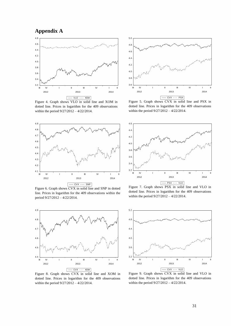
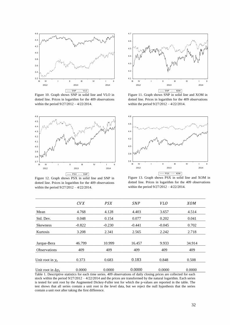
appropriate to conduct some inspection of the data, both visually and formally. In Appendix

A, each pair is presented with graphs for the full period, together with descriptive statistics for

each series. From the graphs for the pairs of SNP – VLO, PSX – VLO and the last year of

SNP – VLO it is possible to see that the series seem to move together, this might however be

spurious given that both series are non-stationary. Table 1 presents the companies with their

respective symbol and also the results of the Augmented Dickey-Fuller test, showing the

probability of the presence of a unit root in the level data and in the differenced data

respectively. We cannot, for any series, reject the presence of a unit root in the level data.

Once the data is differenced, we can for all series reject the null hypothesis that the series

contain a unit root. Thus, all series are integrated of order one. The ten pairs that can be tested

21

for cointegration are: XOM – SNP, XOM – CVX, XOM – PSX, XOM – VLO, SNP – CVX,

SNP – PSX, SNP – VLO, CVX – PSX, CVX – VLO and PSX – VLO.

Company Symbol Unit root in Unit root in Order of integration

Exxon Mobil Corp. XOM 0.508 0.000 ( )

Sinopec Group SNP 0.183 0.000 ( )

Chevron CVX 0.373 0.000 ( )

Phillips 66 PSX 0.683 0.000 ( )

Valero Energy VLO 0.848 0.000 ( )

Table 1. Reported p-values for the Augmented Dickey-Fuller test on each series, both in level data

and in first difference. For all series, it is shown that we can reject the null hypothesis that the series

contain a unit root after taking the first difference, therefore all series are integrated of order one. The

data comprise 409 observations for each stock between 9/27/2012 – 4/22/2014.

22

Results

As presented in the previous section, the five time series regarding daily closing prices for

different energy companies are all ( ). The aim of our study is to find a pair that could be

profitable to trade within the frame of statistical arbitrage, where the concept of mean-

reversion is a fundamental aspect of the strategy. In this section we present the results for all

pairwise combinations that have been examined by Johansen’s test and the EG approach. The

tests investigate the existence of cointegrating relationships between the variables.

Cointegration implies that the variables are bound to a long-run equilibrium, which can be

visualized in the mean-reversion of the error term from the long-run relationship. To perform

the Johansen’s test, an unrestricted VAR is first estimated for the pair that is examined. This

is constructed in order to find the appropriate lag length suggested by AIC. The unrestricted

VAR is estimated for a larger number of lags, gradually decreasing the lags to ensure that the

lag length suggested by AIC is consistent. We find that for all the pairs, the lag length 1 is

consistently suggested by the criterion. Therefore, an unrestricted VAR(1) is estimated for all

pairs in order to perform the Johansen’s test. Furthermore, it is also necessary to determine

the model used to assess the cointegrating rank. All models are simultaneously estimated, and

the model suggested by AIC is chosen as the appropriate model for our purpose. The results

from the Johansen’s test are presented below in Table 2.

Pair Johansen’s test of cointegrating rank ̂ stationary applying

EG approach

CVX - PSX No cointegration, No

CVX - SNP No cointegration, No

CVX - VLO No cointegration, No

CVX - XOM No cointegration, No

PSX - SNP No cointegration, No

PSX - VLO One cointegrating relationship, ** Yes

**

PSX - XOM No cointegration, No

SNP - VLO No cointegration, No

SNP - XOM No cointegration, No

VLO - XOM No cointegration, No

Table 2. Each possible pair is tested for cointegration by Johansen’s test and by the EG approach.

The EG approach is employed by estimating , and testing ̂ for stationarity

using ADF. ** indicates significance on the 1% level.

By the Johansen’s test we find that one pair has a cointegrating rank of , significant on

the 1% level, whereas we for all other pairs cannot reject the null hypothesis that no

23

cointegrating relationship exists. The results are supported consistently by both the trace test

and the maximum eigenvalue test. To further ensure our findings, we employ the EG

approach to all pairs. The EG approach is a two-step estimation that involves the estimation

of a residual series from a linear combination of the variables in the pair, which is then tested

for stationarity by the Augmented Dickey-Fuller test.

Dependent variable:

Independent variable Augmented Dickey-Fuller for

estimated residuals ( ̂ )

( ) ( ) ( )

Table 3. The pair consisting of PSX and VLO is examined by the EG approach. The linear combination is

estimated, obtaining the estimated series of ̂ . The residual series is then tested by the ADF test, the p-value

(0.000) strongly rejects the null hypothesis that the series contains a unit root. For regression output, t-statistics are

given within parenthesis. The data comprises 409 observations of PSX and VLO respectively.

Both the Johansen’s test and the EG approach indicated that the variables PSX and VLO are

cointegrated. The results from the EG approach are presented above in Table 3. The linear

combination of the two variables shows a very high coefficient of determination, about 97%.

The Augmented Dickey-Fuller test strongly rejects the null hypothesis of unit root in the

estimated residual series, confirming that the variables are indeed cointegrated and that the

relationship is not spurious. As previously mentioned, the cointegrating relationship will

imply that there is a long-run equilibrium between the variables and that any deviations from

this equilibrium are merely temporary. Figure 1 illustrates this mean-reverting behaviour by

plotting the estimated residuals from the linear combination given in Table 3.

Figure 1. The estimated residuals ( ̂ ) from the OLS are standardized and plotted against time for the period 9/27/2012 – 4/22/2014.

The graph shows how deviations from the long-run equilibrium are corrected by

the mean-reverting behaviour of the series. Figure 14 in Appendix shows the

actual series plotted against the fitted series, along with the residuals.

24

Vector Error-Correction

By now we have obtained significant results from both the Johansen’s test and the EG

approach that the variables PSX and VLO are cointegrated. Also, the visual inspection of the

error term from the linear combination has indicated the mean-reverting characteristic of a

cointegrated pair. We are now confident to estimate the VECM from which we can assess

both the short-run and the long-run dynamics of the relationship. As indicated in the

unrestricted VAR we employ a lag length of one lag and a model that allows for an intercept

in the cointegrating equation and in the VAR, but not for a linear trend in the cointegrating

equation, nor in the VAR. The estimates of the VECM are given below in Table 4.

Cointegrating equation

1.000

-1.342 [-26.996]**

1.885

Error-correction:

Cointegrating equation

-0.012[-0.459]

0.066 [ 2.908]**

0.023 [ 0.309] -0.010 [-0.154]

-0.008 [-0.090] 0.072 [ 0.967]

0.002 [ 1.599] 0.001 [ 1.544]

Table 4. The table reports the estimates for the vector error-correction model for

PSX and VLO, t-statistics within brackets. The cointegrating vector that gives a

stationary combination of the two non-stationary variables constructs the

cointegrating equation. ** indicates significance on the 1% level.

For a cointegrated set of variables, we expect that at least one of the coefficients in the ( )

vector is significantly different from zero. The coefficients in the vector give the so-called

speed of adjustment when any of the variables in the systems causes a deviation from the

long-run equilibrium. If none of the coefficients are different from zero, the error-correction

part falls out and the model no longer supports the concept of cointegration. In our VECM,

vector is given by the two coefficients for the Cointegrating equation, -0.012 and 0.066,

where only the latter is significantly different from zero. This indicates that we have a long-

run relationship between the variables, as we expected given the preceding results. However,

only PSX is responsible for correcting the deviations that might occur from the long-run

equilibrium. As the coefficient for the Cointegrating equation for is not significantly

different from zero, the variable is considered to be weakly exogenous and its whole equation

can be dropped, although it can still be a part of the equation for . The significance of

the coefficient for the error-correction part in the equation for indicates the

unidirectional Granger causality that runs from to .

25

Thus far we have concluded that the VECM supports a long-run relationship between the

variables, where PSX is responsible for correcting any deviations from the long-run

equilibrium. The speed of this adjustment is given by its coefficient for the Cointegrating

equation. Although this is considered to be the essence of the error-correction representation,

the VECM also allows us to assess the short-term dynamics between the variables. By

studying the ( ) matrix of -coefficients for the lagged differences of the variables, the

impact of the short-term effects can be measured. In our case none of the coefficients show

any significant deviation from zero, thereby suggesting that there is no short-run effect

supported by the VECM.

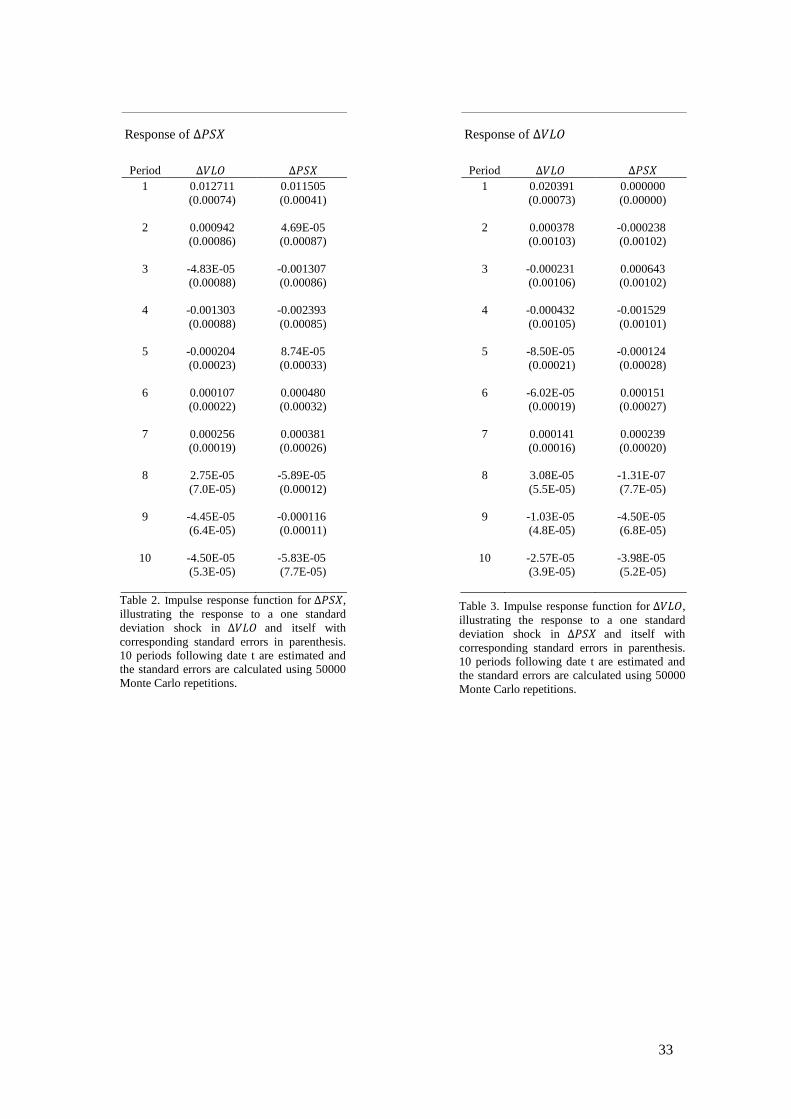
Impulse Response

In the previous section we established that our model is characterized by a mean-reverting

behaviour through the error-correcting term in the VECM, which confirmed the long-term

relationship of the system. To further investigate the short-term behaviour we assess the

Impulse Response Function as mentioned in the theoretical section. Furthermore, we saw that

VLO Granger causes PSX, however the direction alone does not tell us the full story

regarding the interaction of the variables. If one of our stocks responds to an exogenous shock

in the other stock, we may very well draw the conclusion that the latter causes the former,

here we expand on this interaction using IR. Recall that the Vector Moving-Average could be

obtained through an inversion of the VAR model and that the coefficient matrix of the

Moving-Average process contains the responses to a unit-shock. Since the inversion requires

stationary variables it is important to point out that the marginal impact of the shock in each

subsequent time period will tend towards zero over time. An intuitive way of observing the

dynamic interrelationship within the system is to depict a graphical interpretation of a shock

in each of the variables and the corresponding responses for all the variables in the system.

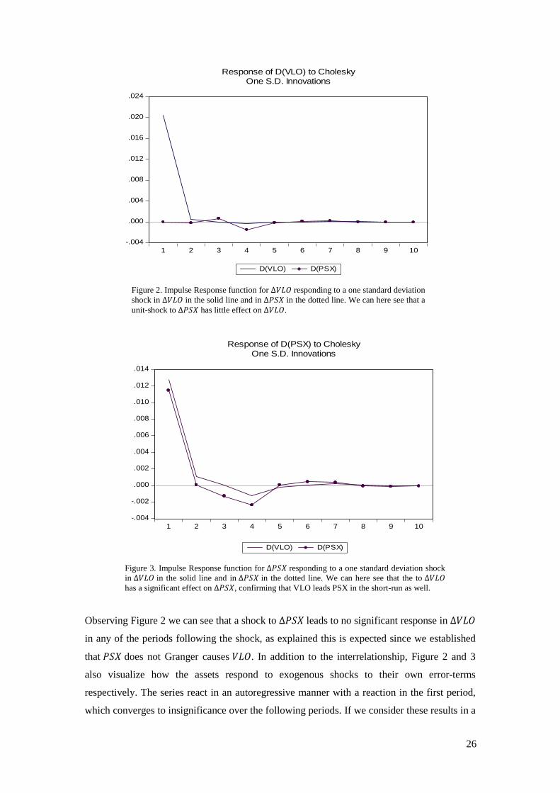
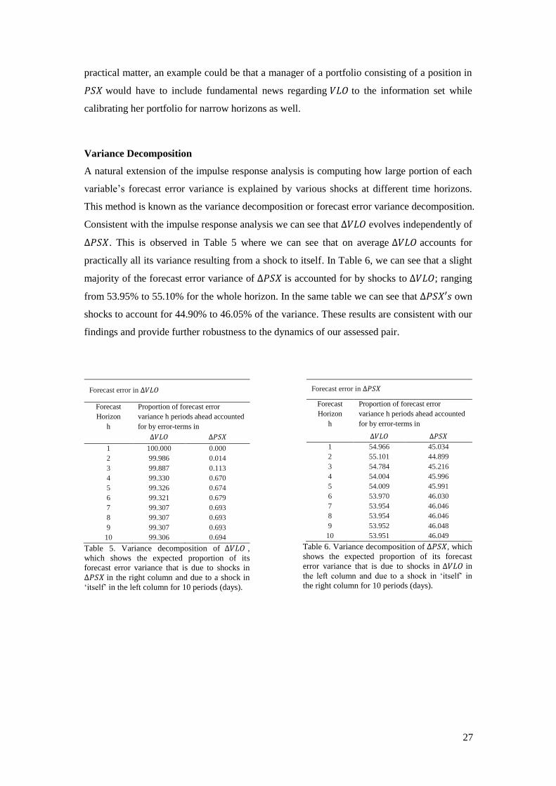
As we can see below in Figure 3, a unit standard deviation shock to leads to an

expected increase of approximately 130 basis points in after one period and in the

subsequent period this significant effect is expected to decrease to approximately 10 basis

points. From the third period and on the effect is insignificant as seen in Table 2 in Appendix

A. As we can see in both Figure 2 and Figure 3, the autoregressive nature of our system

attributes to that there is a convergence to zero rather than the effect seizing immediately.

However, the convergence materializes in rapid manner, showcasing the stability of our

system.

26

-.004

.000

.004

.008

.012

.016

.020

.024

1 2 3 4 5 6 7 8 9 10

D(VLO) D(PSX)

Response of D(VLO) to CholeskyOne S.D. Innovations

Figure 2. Impulse Response function for responding to a one standard deviation

shock in in the solid line and in in the dotted line. We can here see that a

unit-shock to has little effect on .

Figure 3. Impulse Response function for responding to a one standard deviation shock

in in the solid line and in in the dotted line. We can here see that the to

has a significant effect on , confirming that VLO leads PSX in the short-run as well.

Observing Figure 2 we can see that a shock to leads to no significant response in

in any of the periods following the shock, as explained this is expected since we established

that does not Granger causes . In addition to the interrelationship, Figure 2 and 3

also visualize how the assets respond to exogenous shocks to their own error-terms

respectively. The series react in an autoregressive manner with a reaction in the first period,

which converges to insignificance over the following periods. If we consider these results in a

-.004

-.002

.000

.002

.004

.006

.008

.010

.012

.014

1 2 3 4 5 6 7 8 9 10

D(VLO) D(PSX)

Response of D(PSX) to CholeskyOne S.D. Innovations

27

practical matter, an example could be that a manager of a portfolio consisting of a position in

would have to include fundamental news regarding to the information set while

calibrating her portfolio for narrow horizons as well.

Variance Decomposition

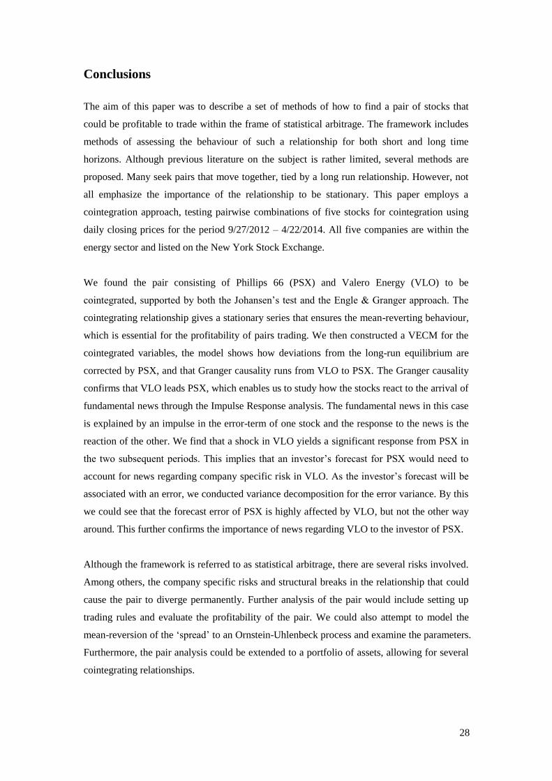
A natural extension of the impulse response analysis is computing how large portion of each

variable’s forecast error variance is explained by various shocks at different time horizons.

This method is known as the variance decomposition or forecast error variance decomposition.

Consistent with the impulse response analysis we can see that evolves independently of

. This is observed in Table 5 where we can see that on average accounts for

practically all its variance resulting from a shock to itself. In Table 6, we can see that a slight

majority of the forecast error variance of is accounted for by shocks to ; ranging

from 53.95% to 55.10% for the whole horizon. In the same table we can see that own

shocks to account for 44.90% to 46.05% of the variance. These results are consistent with our

findings and provide further robustness to the dynamics of our assessed pair.

Forecast error in

Forecast

Horizon

h

Proportion of forecast error

variance h periods ahead accounted

for by error-terms in

1 100.000 0.000

2 99.986 0.014

3 99.887 0.113

4 99.330 0.670

5 99.326 0.674

6 99.321 0.679

7 99.307 0.693

8 99.307 0.693

9 99.307 0.693

10 99.306 0.694

Table 5. Variance decomposition of ,

which shows the expected proportion of its

forecast error variance that is due to shocks in

in the right column and due to a shock in

‘itself’ in the left column for 10 periods (days).

Forecast error in

Forecast

Horizon

h

Proportion of forecast error

variance h periods ahead accounted

for by error-terms in

1 54.966 45.034

2 55.101 44.899

3 54.784 45.216

4 54.004 45.996

5 54.009 45.991

6 53.970 46.030

7 53.954 46.046

8 53.954 46.046

9 53.952 46.048

10 53.951 46.049

Table 6. Variance decomposition of , which

shows the expected proportion of its forecast

error variance that is due to shocks in in

the left column and due to a shock in ‘itself’ in

the right column for 10 periods (days).

28

Conclusions

The aim of this paper was to describe a set of methods of how to find a pair of stocks that

could be profitable to trade within the frame of statistical arbitrage. The framework includes

methods of assessing the behaviour of such a relationship for both short and long time

horizons. Although previous literature on the subject is rather limited, several methods are

proposed. Many seek pairs that move together, tied by a long run relationship. However, not

all emphasize the importance of the relationship to be stationary. This paper employs a

cointegration approach, testing pairwise combinations of five stocks for cointegration using

daily closing prices for the period 9/27/2012 – 4/22/2014. All five companies are within the

energy sector and listed on the New York Stock Exchange.

We found the pair consisting of Phillips 66 (PSX) and Valero Energy (VLO) to be

cointegrated, supported by both the Johansen’s test and the Engle & Granger approach. The

cointegrating relationship gives a stationary series that ensures the mean-reverting behaviour,

which is essential for the profitability of pairs trading. We then constructed a VECM for the

cointegrated variables, the model shows how deviations from the long-run equilibrium are

corrected by PSX, and that Granger causality runs from VLO to PSX. The Granger causality

confirms that VLO leads PSX, which enables us to study how the stocks react to the arrival of

fundamental news through the Impulse Response analysis. The fundamental news in this case

is explained by an impulse in the error-term of one stock and the response to the news is the

reaction of the other. We find that a shock in VLO yields a significant response from PSX in

the two subsequent periods. This implies that an investor’s forecast for PSX would need to

account for news regarding company specific risk in VLO. As the investor’s forecast will be

associated with an error, we conducted variance decomposition for the error variance. By this

we could see that the forecast error of PSX is highly affected by VLO, but not the other way

around. This further confirms the importance of news regarding VLO to the investor of PSX.

Although the framework is referred to as statistical arbitrage, there are several risks involved.

Among others, the company specific risks and structural breaks in the relationship that could

cause the pair to diverge permanently. Further analysis of the pair would include setting up

trading rules and evaluate the profitability of the pair. We could also attempt to model the

mean-reversion of the ‘spread’ to an Ornstein-Uhlenbeck process and examine the parameters.

Furthermore, the pair analysis could be extended to a portfolio of assets, allowing for several

cointegrating relationships.

29

Bibliography

Asteriou, D. and Hall, S. (2011), Applied Econometrics, Palgrave Macmillan, New York, 2nd

Edition

Demiralp, S. and Hoover, K. (2003), “Searching for the Causal Structure of Vector Autoregression”,

Oxford bulletin of Economics and Statistics vol. 65, pp. 745-767

Do, B., Faff, R. and Hamza, K. (2006), “A New Approach to Modelling and Estimation for Pairs Trading”,

Working Paper, Monash University

Floros, C. and Vougas, D. (2008), “The Efficiency of Greek Stock Index Futures Market”, Managerial

Finance vol. 24, pp. 498-519

Gatev, E., Goetzmann, W. and Rouwenhorst, G. (2006), “Pairs Trading: Performance of a Relative-Value

Arbitrage Rule”, The Review of Financial Studies vol. 19, pp. 797-827

Granger, C. (1981), “Some Properties of Time Series Data and their Use in Econometric Model

Specification”, Journal of Econometrics vol. 16, pp. 131-130

Granger, C. and Engle, R. (1987), “Co-integration and Error Correction: Representation, Estimation, and

Testing”, Econometrica vol. 55, pp. 251-276

Hamilton, J. (1994), Time Series Analysis, Princeton University Press, New Jersey, 1st Edition

Jacobsen, B. (2008), “Demonstrating Error-Correction Modelling for Intraday Statistical Arbitrage”,

Applied Financial Economics Letters vol. 4, pp. 287-292

Johansen, S. (1998), “Statistical Analysis of Cointegration Vectors”, Journal of Economics Dynamics and

Control vol. 12, pp. 169-210.

Johansen, S. and Juselius, K. (1990), “The Maximum Likelihood Estimation and Inference on

Cointegration – with Application to Demand for Money”, Oxford Bulletin of Economics and Statistics vol.

52, pp. 169-210

Keating, J. (1992), “Structural Approaches to Vector Autoregressions”, Federal Reserve Bank of St. Louis

Review, September/October vol 72 pp. 37-57

Knif, J. and Pynnönen, S. (1999), “Local and Global Price Memory of International Stock Markets”,

Journal of International Financial Markets, Institutions and Money vol. 9, pp. 129-147

Lütkepohl, H. (2005), New Introduction to Multiple Time Series Analysis, Springer-Verlag, Berlin

Heidelberg

MacKinnon, J. (1991), “Critical Values for Cointegration Tests”, Long-run Economic Relationships:

Readings in Cointegration Oxford: Oxford University Press

Manganelli, S. (2002), “Duration, Volume and Volatility Impact of Trades”, ECB Working Paper Series

no. 125

Morin, N. (2006), “Likelihood Ratio Tests on Cointegration Vectors, Disequilibrium Adjustment Vectors,

and their Orthogonal Complements”, Finance and Economics Discussion Series

30

Ross, S. (1976), “The Arbitrage Theory of Capital Asset Pricing”, Journal of Economic Theory vol. 13, pp.

341-360

Ross, S., Roll, R. and Chen, N. (1986), “Economic Forces and the Stock Market”, The Journal of Business

vol. 59, pp. 383-403

Seymen, A. (2008), “A Critical Note on the Forecast Error Variance Decomposition”, Centre for

European Economic Research Discussion Paper No. 08-065

Sims, C. (1980), “Macroeconomics and Reality”, Econometrica vol. 48, pp. 1-48

Stevans, L. and Sessions, D. (2010), “Calculating and Interpreting Multipliers in the Presence of Non-

Stationary Time Series: The Case of U.S. Federal Infrastructure Spending”, American Journal of Social

and Management Sciences vol. 1 No.1, pp. 24-38

Vidyamurthy, G. (2004), Pairs Trading: Quantitative Methods and Analysis, John Wiley & Sons, Inc.,

Hoboken, New Jersey

31

Appendix A

Figure 4. Graph shows VLO in solid line and XOM in

dotted line. Prices in logarithm for the 409 observations

within the period 9/27/2012 – 4/22/2014.

Figure 5. Graph shows CVX in solid line and PSX in

dotted line. Prices in logarithm for the 409 observations

within the period 9/27/2012 – 4/22/2014.

Figure 6. Graph shows CVX in solid line and SNP in dotted

line. Prices in logarithm for the 409 observations within the

period 9/27/2012 – 4/22/2014.

Figure 7. Graph shows PSX in solid line and VLO in

dotted line. Prices in logarithm for the 409 observations

within the period 9/27/2012 – 4/22/2014.

Figure 8. Graph shows CVX in solid line and XOM in

dotted line. Prices in logarithm for the 409 observations

within the period 9/27/2012 – 4/22/2014.

Figure 9. Graph shows CVX in solid line and VLO in

dotted line. Prices in logarithm for the 409 observations

within the period 9/27/2012 – 4/22/2014.

3.2

3.4

3.6

3.8

4.0

4.2

4.4

4.6

4.8

III IV I II III IV I II

2012 2013 2014

VLO XOM

3.6

3.8

4.0

4.2

4.4

4.6

4.8

5.0

III IV I II III IV I II

2012 2013 2014

CVX PSX

4.1

4.2

4.3

4.4

4.5

4.6

4.7

4.8

4.9

III IV I II III IV I II

2012 2013 2014

CVX SNP

3.2

3.4

3.6

3.8

4.0

4.2

4.4

4.6

III IV I II III IV I II

2012 2013 2014

PSX VLO

4.4

4.5

4.6

4.7

4.8

4.9

III IV I II III IV I II

2012 2013 2014

CVX XOM

3.2

3.6

4.0

4.4

4.8

5.2

III IV I II III IV I II

2012 2013 2014

CVX VLO

32

Figure 10. Graph shows SNP in solid line and VLO in

dotted line. Prices in logarithm for the 409 observations

within the period 9/27/2012 – 4/22/2014.

Figure 11. Graph shows SNP in solid line and XOM in

dotted line. Prices in logarithm for the 409 observations

within the period 9/27/2012 – 4/22/2014.

Figure 12. Graph shows PSX in solid line and SNP in

dotted line. Prices in logarithm for the 409 observations

within the period 9/27/2012 – 4/22/2014.

Figure 13. Graph shows PSX in solid line and XOM in

dotted line. Prices in logarithm for the 409 observations

within the period 9/27/2012 – 4/22/2014.

Mean 4.768 4.128 4.403 3.657 4.514

Std. Dev. 0.048 0.154 0.077 0.202 0.041

Skewness -0.822 -0.230 -0.441 -0.045 0.702

Kurtosis 3.208 2.341 2.565 2.242 2.718

Jarque-Bera 46.799 10.999 16.457 9.933 34.914

Observations 409 409 409 409 409

Unit root in

0.373

0.683

0.183

0.848

0.508

Unit root in

0.0000

0.0000

0.0000

0.0000

0.0000

Table 1. Descriptive statistics for each time series. 409 observations of daily closing prices are collected for each

stock within the period 9/27/2012 – 4/22/2014 and the prices are transformed by the natural logarithm. Each series

is tested for unit root by the Augmented Dickey-Fuller test for which the p-values are reported in the table. The

test shows that all series contain a unit root in the level data, but we reject the null hypothesis that the series

contain a unit root after taking the first difference.

3.2

3.4

3.6

3.8

4.0

4.2

4.4

4.6

III IV I II III IV I II

2012 2013 2014

SNP VLO

4.1

4.2

4.3

4.4

4.5

4.6

4.7

III IV I II III IV I II

2012 2013 2014

SNP XOM

3.7

3.8

3.9

4.0

4.1

4.2

4.3

4.4

4.5

4.6

III IV I II III IV I II

2012 2013 2014

PSX SNP

3.6

3.8

4.0

4.2

4.4

4.6

4.8

III IV I II III IV I II

2012 2013 2014

PSX XOM

33

Table 2. Impulse response function for ,

illustrating the response to a one standard

deviation shock in and itself with

corresponding standard errors in parenthesis.

10 periods following date t are estimated and

the standard errors are calculated using 50000

Monte Carlo repetitions.

Response of

Period

1

2

3

4

5

6

7

8

9

10

0.012711

(0.00074)

0.000942

(0.00086)

-4.83E-05

(0.00088)

-0.001303

(0.00088)

-0.000204

(0.00023)

0.000107

(0.00022)

0.000256

(0.00019)

2.75E-05

(7.0E-05)

-4.45E-05

(6.4E-05)

-4.50E-05

(5.3E-05)

0.011505

(0.00041)

4.69E-05

(0.00087)

-0.001307

(0.00086)

-0.002393

(0.00085)

8.74E-05

(0.00033)

0.000480

(0.00032)

0.000381

(0.00026)

-5.89E-05

(0.00012)

-0.000116

(0.00011)

-5.83E-05

(7.7E-05)

Table 3. Impulse response function for ,

illustrating the response to a one standard

deviation shock in and itself with

corresponding standard errors in parenthesis.

10 periods following date t are estimated and

the standard errors are calculated using 50000

Monte Carlo repetitions.

Response of

Period

1

2

3

4

5

6

7

8

9

10

0.020391

(0.00073)

0.000378

(0.00103)

-0.000231

(0.00106)

-0.000432

(0.00105)

-8.50E-05

(0.00021)

-6.02E-05

(0.00019)

0.000141

(0.00016)

3.08E-05

(5.5E-05)

-1.03E-05

(4.8E-05)

-2.57E-05

(3.9E-05)

0.000000

(0.00000)

-0.000238

(0.00102)

0.000643

(0.00102)

-0.001529

(0.00101)

-0.000124

(0.00028)

0.000151

(0.00027)

0.000239

(0.00020)

-1.31E-07

(7.7E-05)

-4.50E-05

(6.8E-05)

-3.98E-05

(5.2E-05)

34

-.12

-.08

-.04

.00

.04

.08

3.6

3.8

4.0

4.2

4.4

4.6

III IV I II III IV I II

2012 2013 2014

Residual Actual Fitted

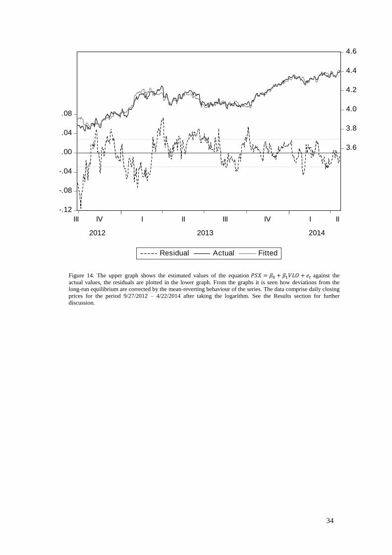
Figure 14. The upper graph shows the estimated values of the equation against the

actual values, the residuals are plotted in the lower graph. From the graphs it is seen how deviations from the

long-run equilibrium are corrected by the mean-reverting behaviour of the series. The data comprise daily closing

prices for the period 9/27/2012 – 4/22/2014 after taking the logarithm. See the Results section for further

discussion.