on multivariate polynomial interpolation. subject the purpose of this work is to provide the problem...
Post on 22-Dec-2015
230 views
TRANSCRIPT
ON MULTIVARIATE
POLYNOMIAL
INTERPOLATION
Subject
The purpose of this work is to provide the problem of
Hermite-Lagrange multivariate polynomial interpolation and
especially the computation of the inverse of a two variable
polynomial matrix.
We start the presentation stating some basic definitions
for univariate case.
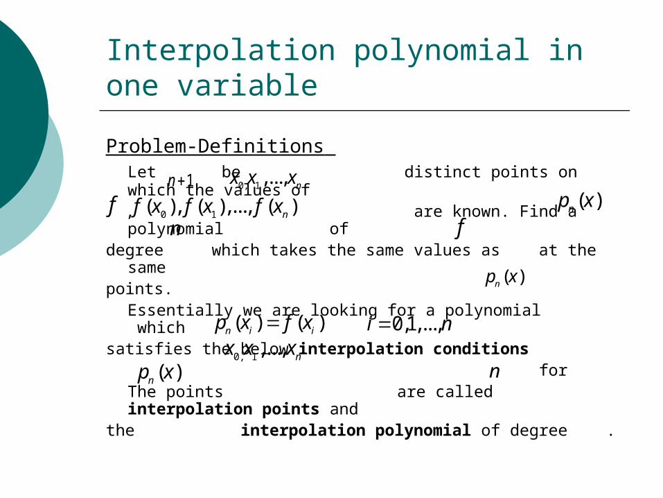
Interpolation polynomial in one variable
Problem-Definitions Let be distinct points on which the values of
, are known. Find a polynomial of degree which takes the same values as at the same points.
Essentially we are looking for a polynomial which satisfies the below interpolation conditions for
The points are called interpolation points andthe interpolation polynomial of degree .
1n 0, 1,..., nx x x
0 1( ), ( ),..., ( )nf x f x f xf ( )np xf
( )np x
( ) ( )n i ip x f x 0,1,...,i n0, 1,..., nx x x
( )np x n
n
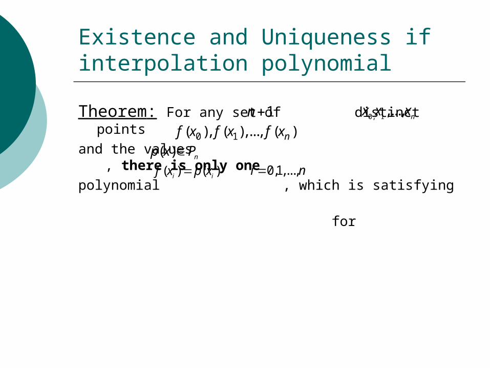
Existence and Uniqueness if interpolation polynomial
Theorem: For any set of distinct points
and the values , there is only one
polynomial , which is satisfying
for
1n 0, 1,..., nx x x
( ) np x P( ) ( )i if x p x 0,1,...,i n
0 1( ), ( ),..., ( )nf x f x f x
Hermite-Lagrange polynomial interpolation in two variables
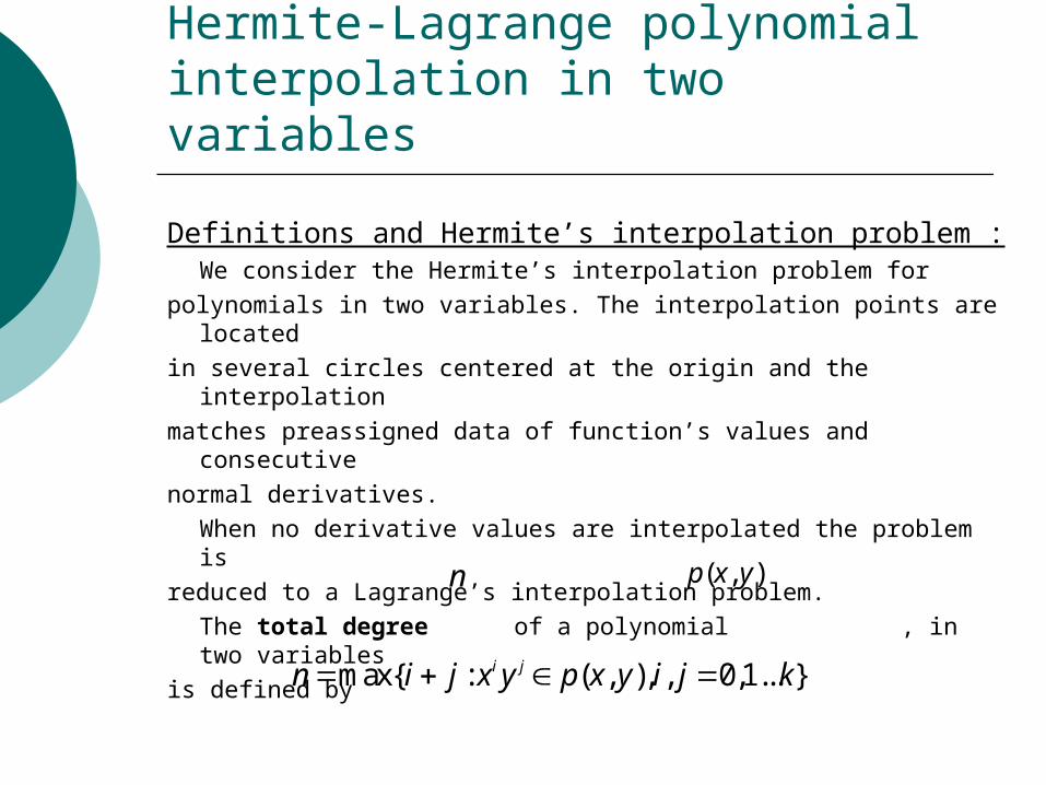
Definitions and Hermite’s interpolation problem :We consider the Hermite’s interpolation problem for
polynomials in two variables. The interpolation points are located
in several circles centered at the origin and the interpolation
matches preassigned data of function’s values and consecutive
normal derivatives. When no derivative values are interpolated the problem is
reduced to a Lagrange’s interpolation problem. The total degree of a polynomial , in two variables
is defined by
( , )p x yn
max{ : ( , ), , 0,1... }i jn i j x y p x y i j k
Hermite-Lagrange polynomial interpolation in two variables
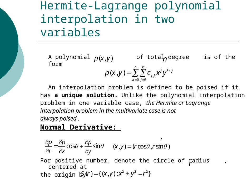
A polynomial of total degree is of the form
An interpolation problem is defined to be poised if it has a unique solution. Unlike the polynomial interpolation problem in one variable case, the Hermite or Lagrange interpolation problem in the multivariate case is not always poised.
Normal Derivative: , For positive number, denote the circle of radius , centered at the origin by
( , )p x y n
,0 0
( , )n k
j k j
j kk j
p x y c x y
cos sinp p p
r x y
( , ) ( cos , sin )x y r r
2 2 2( ) {( , ) : }S r x y x y r r
Hermite-Lagrange polynomial interpolation in two variables
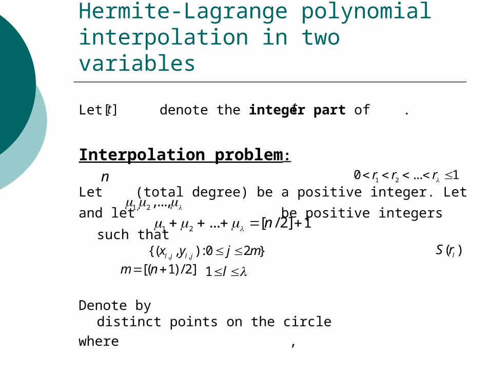
Let denote the integer part of .
Interpolation problem:
Let (total degree) be a positive integer. Let
and let be positive integers such that
Denote by distinct points on the circle
where ,
[ ]t t
n 1 20 ... 1r r r
1, 2 ,...,
1 2 ... [ / 2] 1n
, ,{( , ) : 0 2 }l j l jx y j m ( )lS r
[( 1) / 2]m n 1 l
Hermite-Lagrange polynomial interpolation in two variables
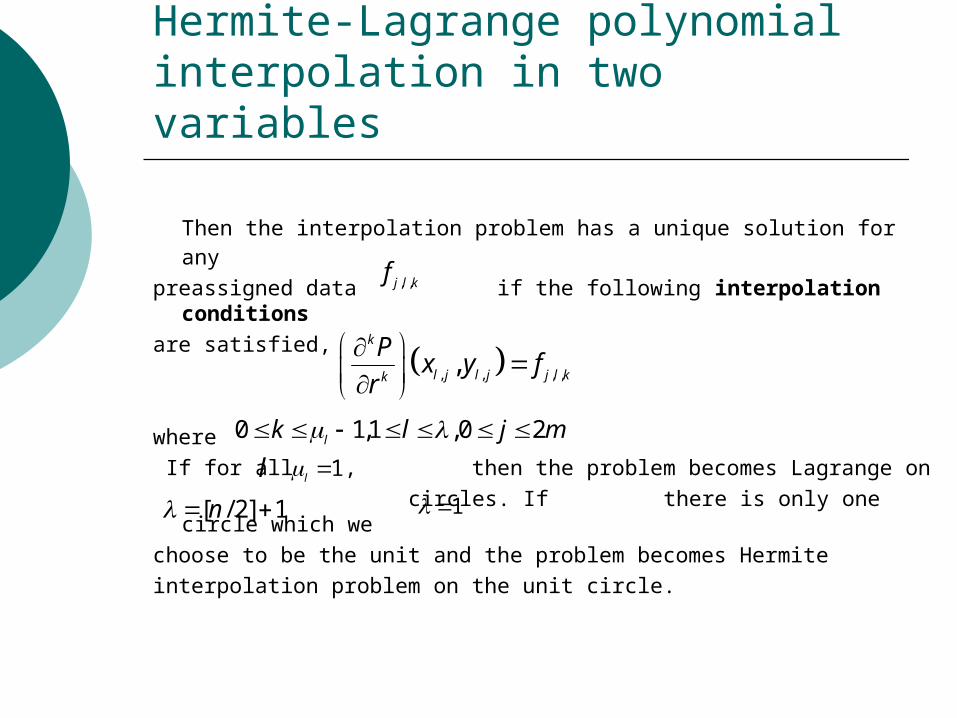
Then the interpolation problem has a unique solution for any
preassigned data if the following interpolation conditions
are satisfied,
where
If for all , then the problem becomes Lagrange on
circles. If there is only one circle which we
choose to be the unit and the problem becomes Hermite
interpolation problem on the unit circle.
, ,j l kf
, , , ,,k
l j l j j l kk
Px y f
r
0 1,1 ,0 2lk l j m
l 1l
[ / 2] 1n 1
Hermite-Lagrange polynomial interpolation in two variables
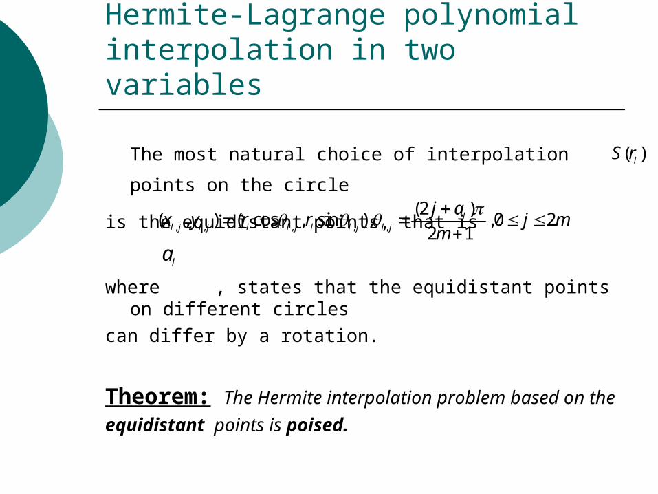
The most natural choice of interpolation points on the circle
is the equidistant points, that is
where , states that the equidistant points on different circles
can differ by a rotation.
Theorem: The Hermite interpolation problem based on the
equidistant points is poised.
( )lS r
, , , , ,
(2 )( , ) ( cos , sin ), ,0 2
2 1l
l j l j l l j l l j l j
j ax y r r j m
m
la
Hermite-Lagrange polynomial interpolation in two variables
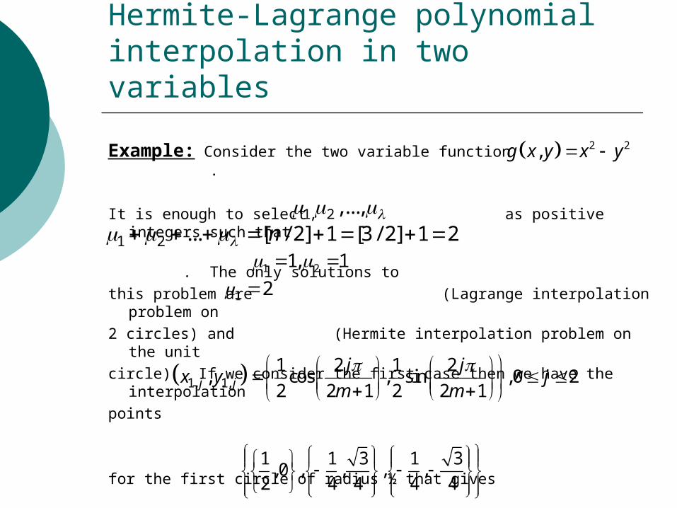
Example: Consider the two variable function .
It is enough to select as positive integers such that
. The only solutions to
this problem are (Lagrange interpolation problem on
2 circles) and (Hermite interpolation problem on the unit
circle) . If we consider the first case then we have the interpolation
points
for the first circle of radius ½ that gives
2 2,g x y x y
1, 2 ,..., 1 2 ... [ / 2] 1 [3 / 2] 1 2n
1 21, 1
1 2
1, 1,1 2 1 2
, cos , sin ,0 22 2 1 2 2 1j j
j jx y j
m m
1 1 3 1 3,0 , , , ,2 4 4 4 4
Hermite-Lagrange polynomial interpolation in two variables
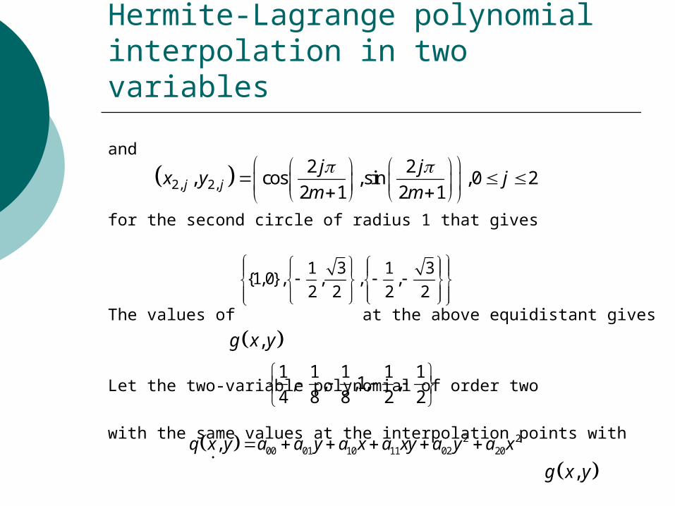
and
for the second circle of radius 1 that gives
The values of at the above equidistant gives
Let the two-variable polynomial of order two
with the same values at the interpolation points with .
2, 2,2 2
, cos ,sin ,0 22 1 2 1j jj j
x y jm m
1 3 1 3{1,0}, , , ,
2 2 2 2
,g x y
1 1 1 1 1, , ,1, ,4 8 8 2 2
2 200 01 10 11 02 20,q x y a a y a x a xy a y a x
,g x y
Hermite-Lagrange polynomial interpolation in two variables
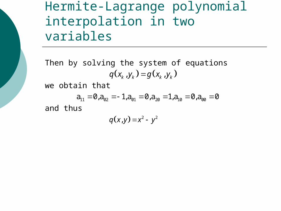
Then by solving the system of equations
we obtain that
and thus
, ,k k k kq x y g x y
11 02 01 20 10 00a 0,a 1,a 0,a 1,a 0,a 0
2 2,q x y x y
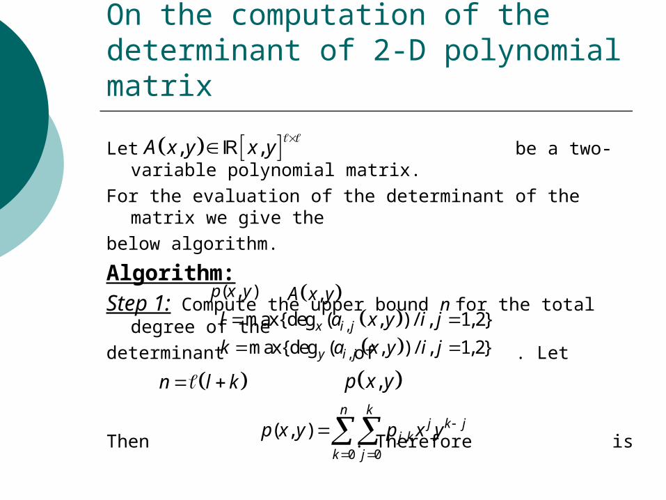
On the computation of the determinant of 2-D polynomial matrix
Let be a two-variable polynomial matrix.
For the evaluation of the determinant of the matrix we give the
below algorithm.
Algorithm:
Step 1: Compute the upper bound n for the total degree of the
determinant of . Let
Then . Therefore is
, ,A x y x y
( , )p x y ,A x y
,max{deg ( , ) / , 1, 2}x i jl a x y i j
,max{deg ( , ) / , 1, 2}y i jk a x y i j
n l k ,p x y
,0 0
( , )n k
j k jj k
k j
p x y p x y
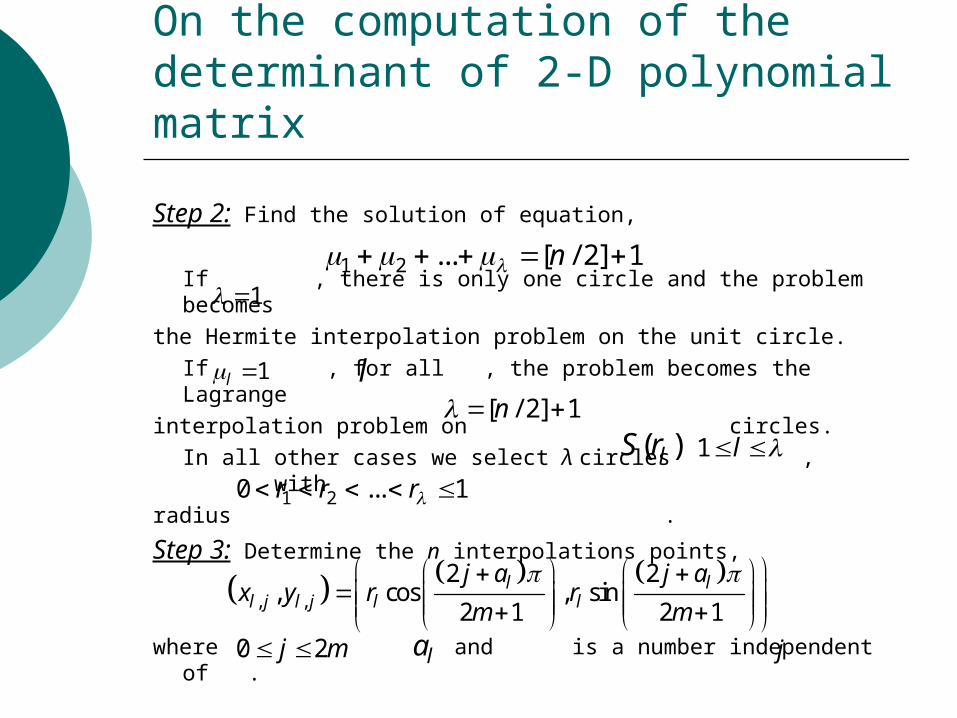
On the computation of the determinant of 2-D polynomial matrix
Step 2: Find the solution of equation,
If , there is only one circle and the problem becomes
the Hermite interpolation problem on the unit circle.
If , for all , the problem becomes the Lagrange
interpolation problem on circles.
In all other cases we select λ circles , with
radius .
Step 3: Determine the n interpolations points,
where and is a number independent of .
1 2 ... [ / 2] 1n 1
1l l[ / 2] 1n
( )lS r 1 l
1 20 ... 1r r r
, ,
2 2, cos , sin
2 1 2 1l l
l j l j l l
j a j ax y r r
m m
0 2j m la j
On the computation of the determinant of 2-D polynomial matrix
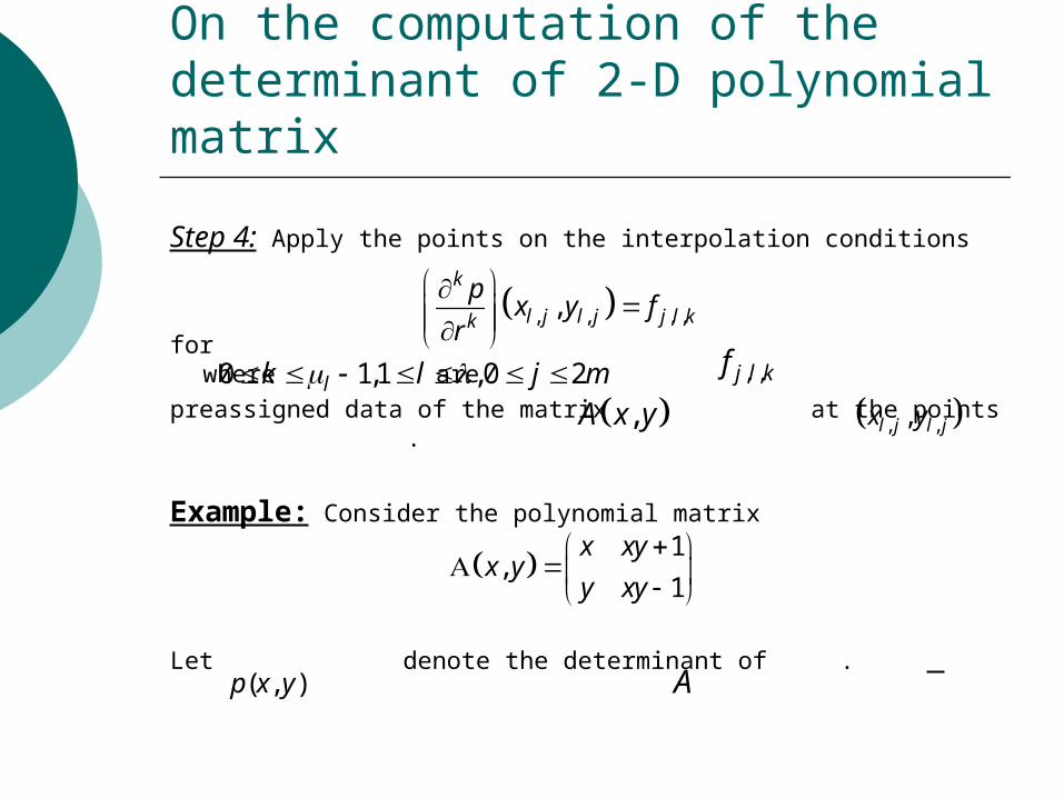
Step 4: Apply the points on the interpolation conditions
for where are
preassigned data of the matrix at the points .
Example: Consider the polynomial matrix
Let denote the determinant of .
, , , ,,k
l j l j j l kk
px y f
r
0 1,1 ,0 2lk l j m , ,j l kf
,A x y , ,,l j l jx y
1,
1
x xyx y
y xy
( , )p x y A
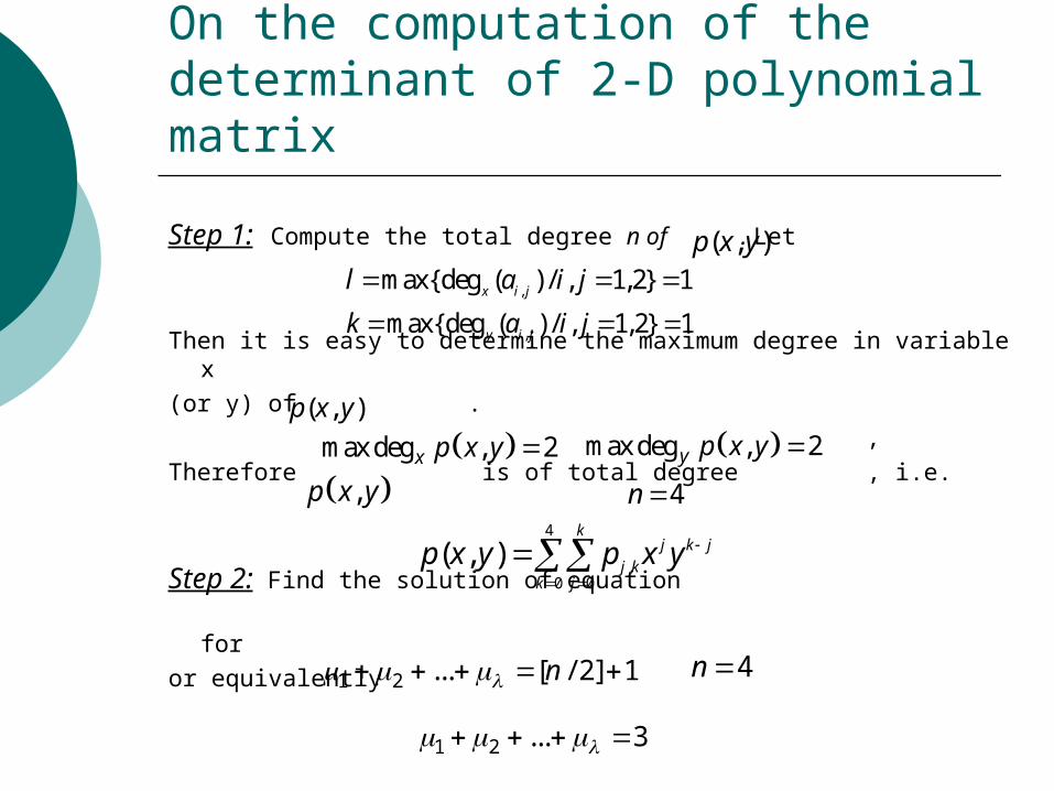
On the computation of the determinant of 2-D polynomial matrix
Step 1: Compute the total degree n of . Let
Then it is easy to determine the maximum degree in variable x
(or y) of .
,
Therefore is of total degree , i.e.
Step 2: Find the solution of equation
for
or equivalently
( , )p x y
,max{deg ( ) / , 1,2} 1x i jl a i j
,max{deg ( ) / , 1,2} 1y i jk a i j
4n4
,0 0
( , )k
j k j
j kk j
p x y p x y
( , )p x y
maxdeg , 2x p x y maxdeg , 2y p x y
,p x y
1 2 ... [ / 2] 1n 4n
1 2 ... 3
On the computation of the determinant of 2-D polynomial matrix
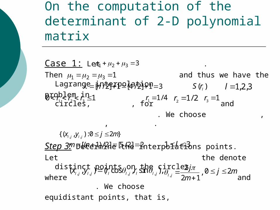
Case 1: Let .
Then and thus we have the Lagrange interpolation
problem in circles, , for and
. We choose , , .
Step 3: Determine the interpolations points.
Let the denote distinct points on the circles
where and . We choose
equidistant points, that is,
( )lS r
1 2 30 1r r r
, ,{( , ) : 0 2 }l j l jx y j m
, , , ,( , ) ( cos , sin ),l j l j l l j l l jx y r r ,
2,
2 1l j
j
m
[( 1) / 2] [5/ 2] 2m n
1,2,3l 1 1/ 4r
2 1/ 2r 3 1r
1 2 3 3
1 2 3 1 [ / 2] 1 [4 / 2] 1 3n
1 3l
0 2j m
On the computation of the determinant of 2-D polynomial matrix
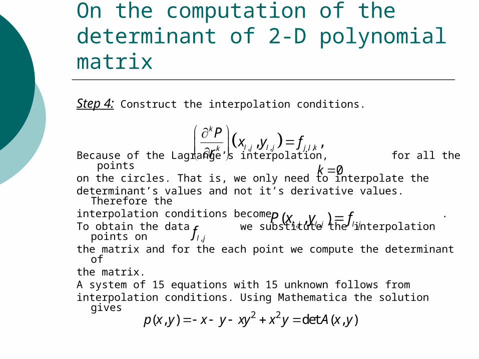
Step 4: Construct the interpolation conditions.
Because of the Lagrange’s interpolation, for all the pointson the circles. That is, we only need to interpolate the determinant’s values and not it’s derivative values. Therefore the interpolation conditions become . To obtain the data we substitute the interpolation points on the matrix and for the each point we compute the determinant of the matrix.A system of 15 equations with 15 unknown follows from interpolation conditions. Using Mathematica the solution gives
, , , ,, ,k
l j l j j l kk
Px y f
r
0k
, , ,( , )l j l j l jP x y f,l jf
2 2( , ) det ( , )p x y x y xy x y A x y
On the computation of the determinant of 2-D polynomial matrix
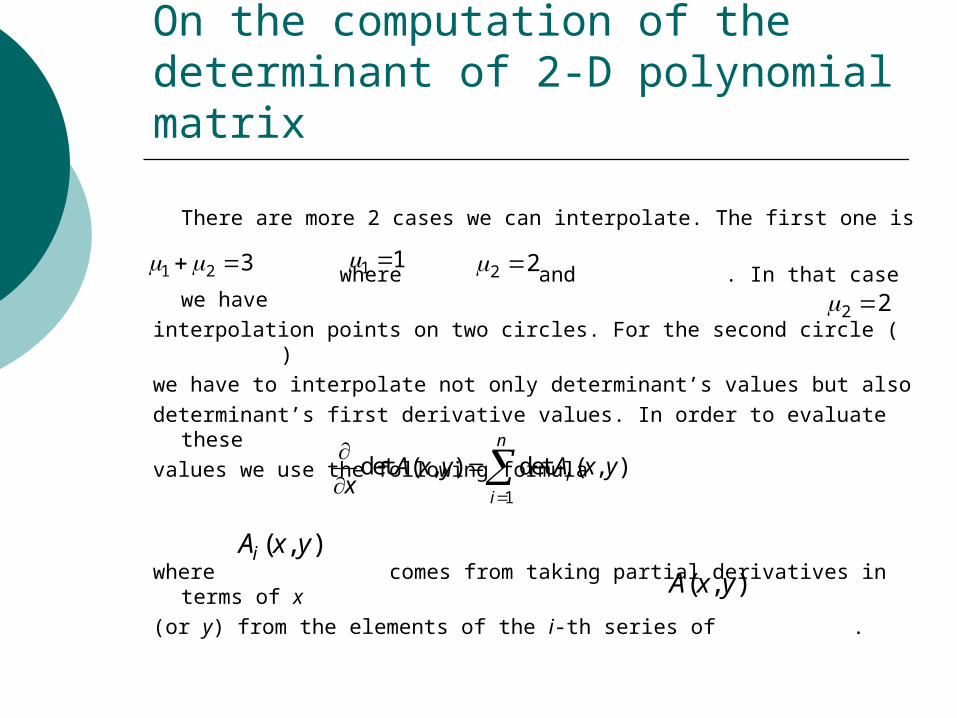
There are more 2 cases we can interpolate. The first one is
where and . In that case we have
interpolation points on two circles. For the second circle ( )
we have to interpolate not only determinant’s values but also
determinant’s first derivative values. In order to evaluate these
values we use the following formula
where comes from taking partial derivatives in terms of x
(or y) from the elements of the i-th series of .
1 2 3 1 1 2 2
2 2
1
det ( , ) det ( , )n
ii
A x y A x yx
( , )iA x y
( , )A x y
On the computation of the determinant of 2-D polynomial matrix
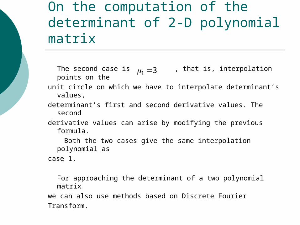
The second case is , that is, interpolation points on the
unit circle on which we have to interpolate determinant’s values,
determinant’s first and second derivative values. The second
derivative values can arise by modifying the previous formula.
Both the two cases give the same interpolation polynomial as
case 1.
For approaching the determinant of a two polynomial matrix
we can also use methods based on Discrete Fourier
Transform.
1 3
On the computation of the determinant of 2-D polynomial matrix
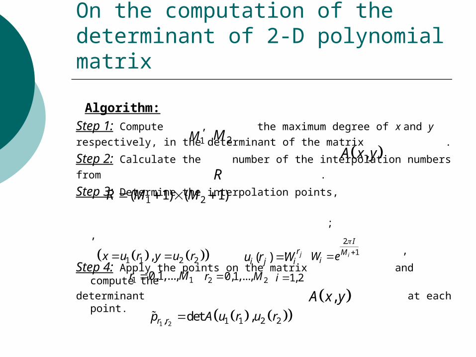
Algorithm:
Step 1: Compute , the maximum degree of x and y
respectively, in the determinant of the matrix .
Step 2: Calculate the number of the interpolation numbers
from .
Step 3: Determine the interpolation points,
; ,
, ,
Step 4: Apply the points on the matrix and compute the
determinant at each point.
1M 2M
,A x y
R
1 2( 1) ( 1)R M M
1 1 2 2,x u r y u r ( ) jri j iu r W
2
1i
I
MiW e
1 10,1,...,r M 2 20,1,...,r M 1,2i
,A x y
1 2, 1 1 2 2det ,r rp A u r u r
On the computation of the determinant of 2-D polynomial matrix
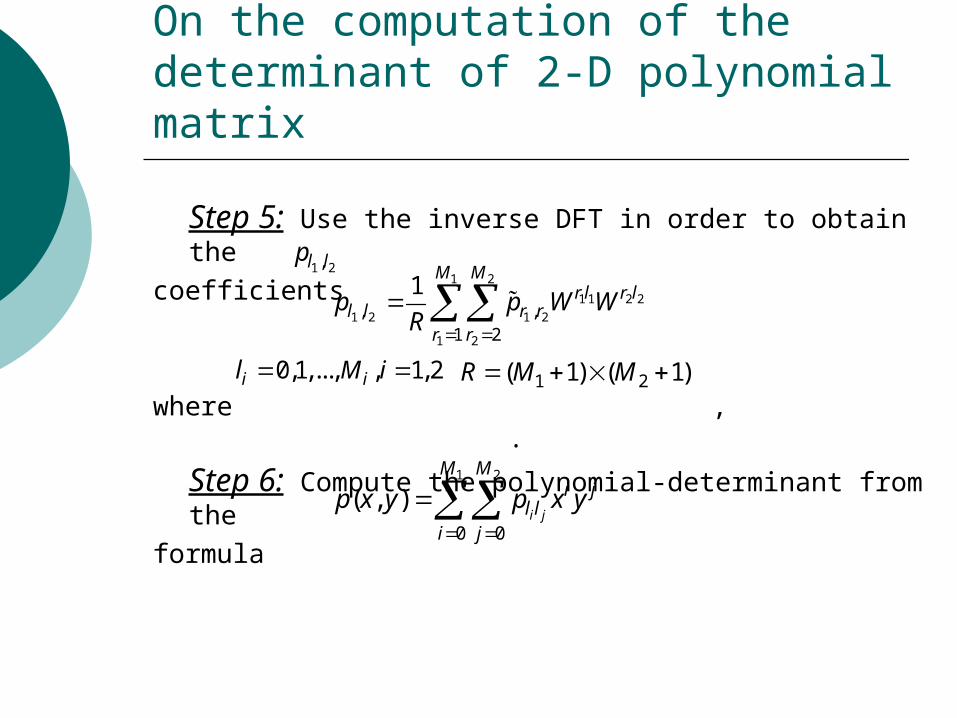
Step 5: Use the inverse DFT in order to obtain the
coefficients
where , .
Step 6: Compute the polynomial-determinant from the
formula
1 2,l lp
1 2
1 1 2 2
1 2 1 2
1 2
, ,1 2
1M M
r l r ll l r r
r r
p p W WR
0,1,..., , 1, 2i il M i 1 2( 1) ( 1)R M M
1 2
0 0
( , )i j
M Mi j
l li j
p x y p x y
Inversion of a 2-D polynomial matrix via interpolation
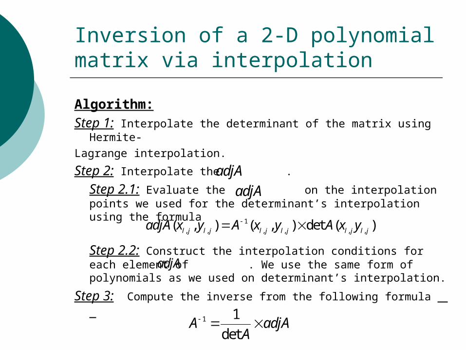
Algorithm:
Step 1: Interpolate the determinant of the matrix using Hermite-
Lagrange interpolation.
Step 2: Interpolate the .
Step 2.1: Evaluate the on the interpolation points we used for the determinant’s interpolation using the formula
Step 2.2: Construct the interpolation conditions for each element of . We use the same form of polynomials as we used on determinant’s interpolation.
Step 3: Compute the inverse from the following formula
adjA
adjA
1
, , , , , ,( , ) ( , ) det ( )l j l j l j l j l j l jadjA x y A x y A x y
adjA
1 1
detA adjA
A