on differential systems with quadratic impulses … · on differential systems with quadratic...

SIAM J. CONTROL AND OPTIMIZATIONVol. 31, No. 5, pp. 1205-1220 September 1993

(1993 Society for Industrial and Applied MathematicsO08

ON DIFFERENTIAL SYSTEMS WITH QUADRATIC IMPULSESAND THEIR APPLICATIONS TO LAGRANGIAN MECHANICS*

ALBERTO BRESSANf AND FRANCO RAMPAZZO:

Abstract. This paper is concerned with the basic dynamics and a class of variational problemsfor control systems of the form

(E) ic f(t, x, u) + g(t, x, u)it + h(t, x, u)/t2

These systems have impulsive character, due to the presence of the time derivative of the control.It is shown that trajectories can be well defined when the controls u are limits (in a suitable weaksense) of sequences (un) contained in the Sobolev space W1,2. Roughly speaking, one can say that,in this case, the/n tend to the square root of a measure. Actually, this paper shows that the system(E) is essentially equivalent to an (affine) impulsive system of the form

c f(x) + g(x)v -t- h(x)v,

where v E L2 and b is a nonnegative Radon measure not smaller than v2. This provides a charac-terization of the closure of the set of trajectories of (E), as the controls u range inside a fixed ballof W1,2. The existence of (generalized) optimal controls for variational problems of Mayer type isalso investigated. Since the main motivation for studying systems of form (E) comes from RationalMechanics, this paper concludes by presenting an example of an impulsive Lagrangian system.

Key words, nonlinear impulsive system, L convergence of solutions, existence of optimalgeneralized controls, Lagrangian mechanical system

AMS subject classifications. 34K35, 49A10, 70D10

1. Introduction and notation. To a mechanical Lagrangian system with N+1degrees of freedom and locally parametrized by coordinates (qi, u), i 1,..., N, onecan superimpose new time-dependent constraints by assigning the motion u(-) of thecoordinate u. This leads to impulsive control systems of the form

(E) f(t, x, u) + g(t, x, u)i + h(t, x, u)2, x(0) 5 e Rn t e [0, T],

where, as customary, the dot denotes differentiation with respect to time. The ap-pellative impulsive control systems is here adopted because of the presence of thederivative of the control on the right-hand sides of the equations. We refer to 6 andto the references quoted there for a detailed description of the mechanical problemsthat motivate the study of equations having the form (E). In particular, (6.1) providesa concrete example where the derivative of the control appears quadratically. Thisequation concerns a swing where, unlike the situation considered in [9], the role ofcontrol is played by the angle formed by the swing and the vertical.

We remark that in the usual applications of control theory to classical mechanicsthe quantities indentified with the controls have the character of forces or torques.This leads to ordinary control equations, which do not contain the derivative of the

1991.*Received by the editors February 6, 1991; accepted for publication (in revised form) April 21,

]Scuola Internationale Superiore di Studi Avanzali, Via Beirut 2, 34014 Trieste, Italy.:Department of Mathematics, University of Padova, Via Belzoni 7, 35131 Padova, Italy.

1205

1206 ALBERTO BRESSAN AND FRANCO RAMPAZZO

control. On the contrary, here the control is one of the positional coordinates of themechanical system E. For example, one could try to guide the entire motion of Ejust by assigning the motion of a part H of E: in this case what one can practicallymeasure is the time evolution of the positions of H, while one does not know the forcesnecessary to generate such evolution, as it would be required by the classical approachof control theory to mechanics.

The important case h -= 0, which occurs in such mechanical applications un-der special assumptions on the geometry of the constraint manifold [14], [15], wasconsidered in [2]-[5], [12], [16]-[18].

The aim of this paper is to provide a definition of solution of (E) valid for thegeneral case, i.e, when the derivative/t appears quadratically, and for a suitably largeclass of inputs u. We study the existence, uniqueness, and continuous dependence(on the controls) for the corresponding Cauchy problem. This allows us to drop theaforementioned technical assumptions on the geometry of the constraint manifold andto cover a very large class of mechanical applications. In particular, all the problemswhere the forces depend on the velocities linearly and quadratically are within thisclass, without any assumption on the geometry of the constraints.

Observe first, that by possibly introducing the variables x t, xn+l u andthe new equations 2 1, 2n+l -/t, it is not restrictive to assume that (E) takes thesimpler form

(1.1) 2 f(X) + g(x)it + h(x)/t2, x(O) - e Rn.

When u is absolutely continuous with square integrable derivative, the solutions of(1.1) are already well defined. In the special case, where h -_- 0, it is known thatthe input-output map : u(.) -- x(.) can be extended continuously to a map fromL([0, T], R) into LI([0, T], Rn). However, as shown in [13], when h 0, such continu-ous extension does not exist. On the other hand, as u ranges within bounded subsetsof the Sobolev space W,2([0, T], R), we show in 2 that the input-output map remainscontinuous also with respect to a new topology T on the space of controls, somewhatweaker than the norm topology. This enables us to embed the map in a largerdomain consisting of couples (v, b), where v e L2([0, T], R) and w is a nondecreasingfunction with the property

b

v2(t) dt <_ w(b) w(a) for all 0 _< a < b _< T.

For any such couple we consider a problem of the form

(1.2) 2 f(x) + g(x)v + h(x)lb, x(0) 5.

We prove that the solution of (1.2) depends continuously on the input pair (v, w),2where v e Lweak([0, T], R) and w e LI([0, T], R). This also provides a characterization

of the Ll-closure of the set of trajectories of (1.1) whenever u ranges inside a fixedball in W1,2([0, T], R).

Furthermore, we prove that the set reached at a time t -, e [0, T], by (gen-eralized) solutions of (1.2) is compact. This guarantees the existence of (generalized)optimal controls for a class of variational problems having a dynamics of the form (E).

In 4, some examples display the difficulties that arise when no bound on theL2 norm of/t is imposed. Still, if the vector field h satisfies a suitable coercivity

QUADRATIC IMPULSES 1207

condition, then Ix(t)l-- cx as f iit(s)12ds -- ; hence, the boundedness of solutionsx(.) automatically implies a bound on II/tllL2.

Finally, an application concerning an optimal control problem for a mechanicalsystem is presented in 5.

The following is a list of the notation that will be used in the next sections.The euclidean norm of a vector y E Rn is written lY[, while B[u, p] denotes the

closed ball centered at y with radius p. For r 1,2,... [r 0] we say that amap f R -, Rm is of class Cr if f is r times continuously differentiable [if f iscontinuous]. When f is at least C1, by Dr(x) we denote the m x / Jacobian matrixof f at the point x e R. IDf(x)l indicates the operator norm of Of(x).

Let h be a C vector field on Rd. As customary, (expth)(x) indicates the valueat time t of the solution of the Cauchy problem

[ h(y), y(O) x.

The differential of the map x - (exp th)(x) is denoted by (exp th),. Observe that, foreach x Rd, (exp th), is a linear map from the tangent space at x into the tangentspace at the point (expth)(x). In particular, if f is a vector field on Rd, one has

(1.3) (expth),f(x) lim(expth)(x + f(x)) (expth)(x) v(t),

e--O "C

where (.) is the solution ofthe linear Cauchy problem

(1.4) i(s) Dh((expsh)(x)) v(s), v(O) f(x).

In the following, Wr,P([a, b], Rd) is the Sobolev space of functions from [a, b] intoRd whose distributional derivatives up to order r belong to Lp. If w is a map from[a, b] into Rd, the total variation of w on the interval [a, b] is written V[a,b](W). Werecall that

where the supremum is taken over all partitions {a to < tl < < tn b} of theinterval [a, hi.

If E is a topological vector space, by E* we denote its topological dual space.The convergence of a sequence (v),_>l to a point v in E is written as v, v, while"--" indicates weak convergence.. Systems wth linear impulses. As a preliminary, we provide a notion ofgeneralized solution to the impulsive Cauchy problem

f f(x) + g(x)v + h(x)(v(2.1)

corresponding to a control pair (v, w)(.), in the case where v e L([0,T], R) and w isa bounded, measurable function. Concerning the vector fields f, g, h we shall assume(H) The maps f, g are C. The vector field h is C2 and complete, i.e., for every x the

map t - (expth)(x) is defined for all t e R.Recalling the notation at (1.3), for a given w [0, T] - R consider the vector

fieldsf(t, y) (exp(-w(t)h)),f ((expw(t)h)(y)),


gw(t, y) (exp(-w(t)h)).g((expw(t)h)(y)).DEFINITION 2.1. A map x: [0, T] R’ is a generalized solution of (2.1) if

(2.2) x(t) (expw(t)h)(y(t)) Vt C [0, T],

where y(.) is a Caratheodory solution of the Cauchy problem

(2.3) u(t)) + a (t,y(0) (exp(-w(0)h))(2).

Remark 2.1. If w is smooth, the above definition is equivalent to the classical one.Theorem 2.2 will show that this is the unique extension to the case where v E L andw is bounded measurable.

Remark 2.2. If w’: [0, T] -. R is a measurable function such that w’(0) w(0)and w’(t) w(t) almost everywhere, then fw’ (t, .) fw(t, .), g’ (t, .) g(t, .) forMmost every t. Hence, the corresponding solutions yt, y of (2.3) coincide. The valueof the solution x(.) of (2.1) at a given time - thus depends only on the L equivalenceclass of v, w and on the values of w at t 0 and at t T.

In the following, when we are interested only in the value of a solution at a singletime T, we thus consider functions v, w defined up to L equivalence on [0, T], with wpointwise determined at t 0, T.

THEOREM 2.1. If the hypotheses (H) hold, then there exists T > 0 such that theCauchy problem (2.1) has a unique generalized solution on [0, ’]. If, in addition, thevector fields f, g, h satisfy the bounds

(2.4) If(x)l < c(1+ Ixl), Ig(x)l < c(1+ Ixl), IDh(x)l < Cfor some constant C and all x R, then the generalized solution of (2.1) exists onthe whole interval [0, T] and is uniquely defined.

Proof. By definition, it is clear that the generalized solution x(.) of (2.1) exists andis unique if and only if the same holds for the solution y(.) of (2.3). For any measurablebounded w(.), the functions fw, gw satisfy the hypotheses of Caratheodory’s theorem.being measurable with respect to t and continuously differentiable with respect to y.Therefore, a unique local solution of (2.3) exists.

Concerning the global existence, if M0,M are constants for which

(2.5) Ih(O)l Mo, Iw(t)l <_ M1 Vt e [0, T],

then the bounds (2.4), (2.5)imply

Ih(y)l <_ Mo + Cly I, I(exp(-w(t)h)).l < aCid(t),,

Mo (eCM 1),I(expw(t)hl(y)l <- eCMIyl +

(2.6)]f(t, y)] I(exp(-w(t)h)).f((expw(t)h)(y))l

( M(eCM--1))_

ecM1. C 1 + ecMI ]y] +

-QUADRATIC IMPULSES 1209

for some constant C1. Similarly,

Ig(t,y)l C2(1 -t-lY[).

Recalling that v e L1, the bounds (2.6) and (2.7) imply the global existence of thesolution y(.) of (2.3), on the interval [0, T].

The following approximation result justifies the notion of generalized solutionintroduced in Definition 2.1.

THEOREM 2.2. Assume that the hypotheses (H) and (2.4) on the vector fieldsf,g,h hold, and let (v,w) be a control pair in L2([O,T],R) L([O,T],R), with wpointwise defined at a given T E [0, T] and at t O. Let (vn, Wn)neN be a sequence ofcontrol pairs in L2 W,2, such that IIv,IIL2 <_ L, 0,T](Wn) <_ L, for some constantL, and

vn v in L2([0, T],R),w w in L([O, T], R).

Moreover, suppose that

Then the (Caratheodory) solutions x of (2.1) corresponding to the control pairs (vn, wn)satisfy

(2.8) Xn x in

where x(.) denotes the generalized solution of (2.1) corresponding to (v, w), pointwisedefined at t T and t O.

Proof. In order to prove (2.8) it will be shown that from every subsequence(Xn’),>l of (X,)n>I one can extract a further subsequence (x)> converging tox in L([0, T], Rn) and pointwise at T.

For every n >_ 1, let y, be the solution of (2.6) corresponding to the control pair(Vn’, Wn’). By the hypotheses on f, g, h and on v, Wn, the variations 0,T](Y’) areuniformly bounded. Hence, by Helley’s theorem, there exists a subsequence (y)>lconverging to a map y pointwise on [0, T]. By possibly extracting a further sub-sequence, we can also assume w(t) --. w(t) for almost every t. We claim thatcoincides with the solution y corresponding to the control pair (v, w). By the unique-ness of solutions of (2.3), this can be established by showing that

yc(t) y(O) + [fw(s, yc(s) + gW(s, y(s))v(s)] ds

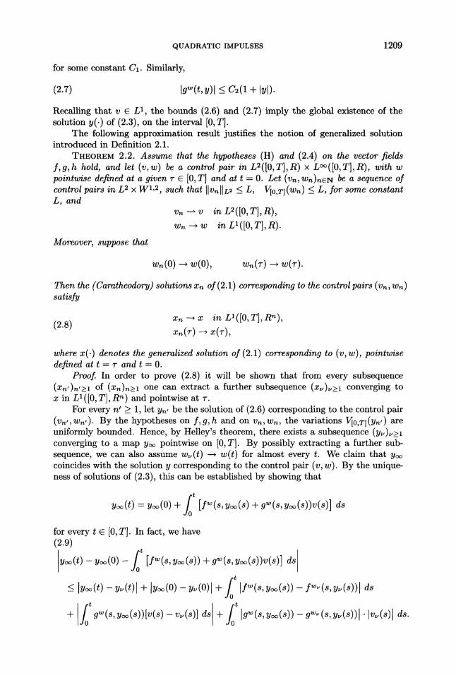
for every t E [0, T]. In fact, we have(2.9)yo(t) yo(O) [f(s, yo(s)) + g(s, yoc(s))v(s)] ds

<_ lyon(t) y(t) + [yo(O) y(O)[ + IfW(s, yo(s)) f(s, y(s)) ds

+ gw(s, yc(s))[v(s) v(s)] ds + Igw(s, yoo(s)) gwv(s,y(s)) Iv(s)l ds.


For every t, as u - cx, the first two terms on the right-hand side of (2.9) convergeto zero. By construction we have fw(s, yv(s)) --, fw(s, yo(s)) for almost every s.Hence, by the Dominated Convergence theorem, the third term on the right-hand sideof (2.9) also converges to zero. The fourth term converges to zero because gW(., y(.))is a bounded function, and the vv converge to v weakly in L2. Finally, the HSlderinequality

Igw(s, y(s)) yw(s, yu(s))] Ivu(s)l ds

<- IIg ( ",

implies that also the fifth term on the right-hand side of (2.9) converges to zero.Indeed, IIvIIL <_ L, and by dominated convergence, g(.,y(.)) - g(.,y(.)) inL2

From the equality y(t) y(t) for every t e [0,T], since wv(t) -- w(t) almosteverywhere and at t T, we obtain that

x(t) (expw(t)h)(y(t)) --. (expw(t)h)(y(t)) x(t)

almost everywhere and at t T. This implies x. -- x in LI([0, T]; R), because the xvare uniformly bounded. Since the subsequence (xn’)n’_>l was arbitrary, the theoremis proved.

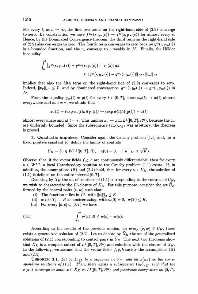
3. Quadratic impulses. Consider again the Cauchy problem (1.1) and, for afixed positive constant K, define the family of controls

UK {u e W1,2([O,T], R), u(0)= 0, II IIn - <Observe that, if the vector fields f, g, h are continuously differentiable, then for everyu E W1,2, a local Caratheodory solution to the Cauchy problem (1.1) exists. If, inaddition, the assumptions (H) and (2.4) hold, then for every u UK, the solution of(1.1) is defined on the entire interval [0, T].

Denoting by XK the set of solutions of (1.1) corresponding to the controls of UK,we wish to characterize the Ll-closure of XK. For this purpose, consider the set UKformed by the control pairs (v, w) such that:

(i) The function v lies in L2, with Ilvll. _< g.(ii) w "[0, T] R is nondecreasing, with w(0)- 0, w(T) <_ K.(iii) For every [a, b] c_ [0, T] we have

(3.1) jfab v2(t) dt <_ w(b)- w(a).

According to the results of the previous section, for every (v, w) UK, thereexists a generalized solution of (2.1). Let us denote by XK the set of the generalizedsolutions of (2.1) corresponding to control pairs in UK. The next two theorems showthat XK is a compact subset of LI([O,T],R) and coincides with the closure of XK.In the following, we assume that the vector fields f, g, h satisfy the assumptions (H)and (2.4).

THEOREM 3.1. Let (Un)n>l be a sequence in UK, and let X(Un) be the corre-sponging solutions of (1.1). Then, there exists a subsequence (u)> such that thex(u,) converge to some x e XK in LI([O,T],Rn) and pointwise everywhere on [0, T].


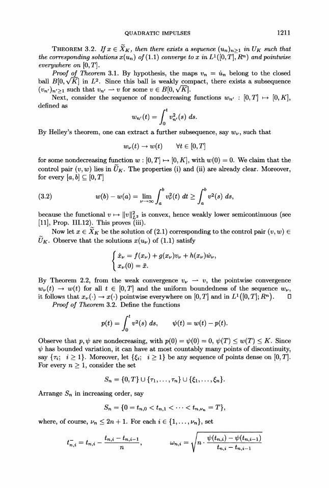
THEOREM 3.2. If x E XK, then there exists a sequence (Un)n>l in UK such thatthe corresponding solutions x(un) of (1.1) converge to x in LI([0, T], Rn) and pointwiseeverywhere on [0, T].

Proof of Theorem 3.1. By hypothesis, the maps vn /tn belong to the closedball B[0, x/] in L2. Since this ball is weakly compact, there exists a subsequence(Vn,),_>i such that v, v for some v E B[0, v/].

Next, consider the sequence of nondecreasing functions Wn, [0, T] - [0, g],defined as

wn, (t) v2n, (s) ds.

By Helley’s theorem, one can extract a further subsequence, say wv, such that

wv(t) --, w(t) Vt e [0, T]for some nondecreasing function w "[0, T] H [0, K], with w(0) 0. We claim that thecontrol pair (v, w) lies in Vg. The properties (i) and (ii) are already clear. Moreover,for every [a, b] c_ [0, T]

(3.2) fab fabw(b)- w(a)= lim v2(t) dt >_ v2(s) ds,

because the functional v livll, is convex, hence weakly lower semicontinuous (see[11], Prop. III.12). This proves (iii).

Now let x XK be the solution of (2.1) corresponding to the control pair (v, w) eUK. Observe that the solutions x(u,) of (1.1) satisfy

f(x) + g(x)vv + h(x)(v,(0) .

By Theorem 2.2, from the weak convergence v v, the pointwise convergencew(t) -- w(t) for all t e [0,T] and the uniform boundedness of the sequence w,it follows that x(.) --. x(.) pointwise everywhere on [0, T] and in L ([0, T]; R=). r3

Proof of Theorem 3.2. Define the functions

p(t) v2(s) ds, (t)

Observe that p, are nondecreasing, with p(0) (0) 0, (T) < w(T) < K. Sincehas bounded variation, it can have at most countably many points of discontinuity,

say {Ti; > 1}. Moreover, let {i; i > 1} be any sequence of points dense on [0,T].For every n > 1, consider the set

Sn {0, T} U {T1,..., Tn} U {,..., =}.Arrange Sn in increasing order, say

S {0 t=,0 < t=, <... < t=,, T},

where, of course, v= _< 2n + 1. For each E {1,..., n}, set

tn,i tn,i-1 (t=,i)--(tn#-i)OJn,i tn,i tn,i-1


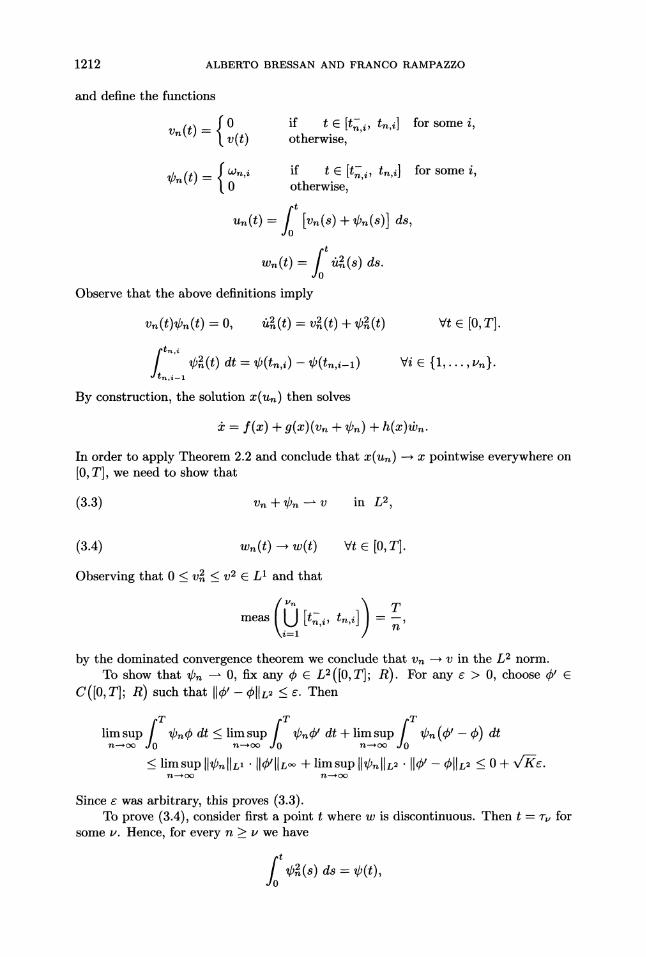
and define the functions

[ 0 if t e [t,i, t,,i]vn(t) v(t) otherwise,for some i,

[ w,,i if t e itS,i, t,i](t) 0 otherwise,

u(t) [v() + ()] ,(t) () d.

Observe that the above definitions imply

for some i,

vn(t)n(t) =0, a(t) (t) + (t) Vt e [0, T].t’

2n(t) dt (tn,i) (t,,i-1)i--1

By construction, the solution x(u) then solves

Vi e {1,...,u}.

f(x) -- R(X)(Vn -- ?n) -- h(x)(v.In order to apply Theorem 2.2 and conclude that x(u) - x pointwise everywhere on[0, T], we need to show that

(3.3) vn + v in L2,

(3.4) w(t) --, w(t) Vt e [0, T].

Observing that 0 _< V2n _< v2 E L and that

meas

by the dominated convergence theorem we conclude that Vn -’+ V in the L2 norm.To show that , 0, fix any e L2 ([0, T]; R). For any e > 0, choose ’C([0, T]; R) such that I1’-IIL --< e. Then

lim sup )n dt <_ lim sup ’ dt + lim sup (’ ) dt

n---c n---o

Since was arbitrary, this proves (3.3).To prove (3.4), consider first a point t where w is discontinuous. Then t T for

some u. Hence, for every n _> p we have

2n(s) ds


while

lim v2 s ds v2 s ds.

Hence, (3.4) holds. The same argument can of course be applied when t 0 or t T.Next, consider the case where w is continuous at t. For any > 0, choose

< t < v such that

< < <

If n > max(p, }, then

2(s) ds- (s) ds,

Hence,

2(s) ds- (t) dr.

w(t)- e < w()= lim w(.) < liminfwn(t)< limsupw,(t) < lim Wn(v) w(t,) <_ w(t) -- .Since e was arbitrary, (3.4) is proved in this case as well.

An application of Theorem 2.2 now implies X(Un)(t) --* x(t) for every t e [0, T],and hence, x(un) -- x in L1, by dominated convergence.

The above results motivate the following definition.DEFINITION 3.1. For every K > 0, UK is called the set of UK-generalized controls

for (1.1), and XK is called the set of UK-generalized trajectories of (1.1).By Theorems 3.1-3.2, a bounded trajectory x is a UK-generalized solution of (1.1)

if and only if x is the pointwise limit of (Caratheodory) solutions of (1.1) correspondingto controls in UK.

In connection with the system (1.1), for any t E [0, T] and K > 0, we also definethe reachable set RK(t) at time t, with generalized controls in UK:

Rg(t) {x(t); x is a solution of (2.1), with (v,w) E g}.From the previous analysis it follows

COROLLARY 3.1. Let the vector fields f,g,h satisfy the assumptions (H) and(2.4). Then, for every T e [0, T] and K > O, the reachable set X:(T) is compact.

Indeed, let (2Cn)n> be a sequence of points in Rg(t). By definition, there exists(wn, wn) e UK such that n X(Vn, Wn)(t). Choose a subsequence (v, w)>l suchthat, for some (v, w) UK, one has

vv--v and w(t) - w(t) Vt e [O,T].

This is possible because the ball B[0, x/-] in L2 is weakly compact and because ofHelly’s theorem. The inequality

b

V2(S) ds < w(b)- w(a)

is then established as in (2.4). By Theorem 2.2 we now have x(v, w)(t) -- x(v, w)(t)for every t. Hence, in particular, the sequence &, converges to x(v, w)(t) Rg(t),proving that RK(T) is compact.


Remark 3.1. The above results remain true if, in place of the hypothesis (2.4),one assumes that all trajectories of (1.1) with u E UK remain inside a fixed compactset S. Indeed, one can then replace the vector fields f, g, h with

where is a C scalar function with compact support such that

(x) _-- 1 if x E S.

Then we can apply all previous results to the system

](x) + +

Remark 3.2. In particular, Corollary 3.1 guarantees the existence of an optimalcontrol for a variational problem of the form

(3.5) min {(I)(x(T)); x K},where (I) Rn H R is lower semicontinuous. Indeed, on the compact set RK(7"), thefunction (I) does attain its global minimum.

4. Controls with bounded variation. By Corollary 3.1, the set 7(T) reachedat t T by the Ug-generalized solutions of (1.1) defined at t T is compact. Thisis no longer true if instead of a bound on the L2 norm of/t only a bound on the totalvariation V[0,T](U), i.e., on the L norm of/t, is imposed: for example, consider thecontrol system

=/t2

x(0) =0

on the time interval [0, 1] and the sequence (Itn)n_>l of controls defined by

nt if t e [0, 1/n],(4.1) un(t) 1 ift e (l/n, 1].

For every n, one trivially has V[O,TI(Un) 1. On the other hand,x(1) n diverges to

It may also happen that the trajectories of (1.1) and the variations of the controlsare uniformly bounded, while the L2 norms of the derivatives of the controls divergeto

For example, consider the control system

(4.2) [ h(x)/t2x(0) R,

where 0 < 121 < 1 and h is the vector field on R2 defined by

+x:+x2(1-x-x)


For a positive constant C, consider the set of admissible controls

U- {u[ u e W1,2([O,T],R), u(O)- 0 0,T](U)- [I/t[[1_

C}.

It is easy to check that for every control u E U the corresponding solution of (4.2)remains inside the closed ball B[0; 1]. As a matter of fact, the circle of equationx 4- x 1 is the w-limit of all trajectories of h starting outside the origin. On theother hand, the controls un defined at (4.1) belong to U with C 1, while their L2

norms ]l/tn[]2 n diverge to +oc.In the case where all positive orbits of h diverge to infinity, however, any bound

on the solutions of (1.1) implies that the L2 norms of the derivatives/t are uniformlybounded as well. Precisely, we have:

THEOREM 4.1. Assume that for every x B[0; R] one has

(4.4) lim I(expth)(x)l c.

Fix C > 0 and define U as the set of all controls u U whose corresponding trajectoryof (1.1) satisfies Ix(u)(t)l < R for all t.

Then, there exists a constant K such that

COROLLARY 4.1. Let X be the set of solutions of (1.1) corresponding to thecontrols belonging to U, defined as in Theorem 4.1, and let - denote its closure inLi([0, T], Rn). If h satisfies (4.4), then

X CXK,

for a suitable constant K. In particular, X is precompact in LI([O,T],Rn).Proof of Theorem 4.1. By (4.4) and by the compactness of B[0; R], there exists a

T > 0 and an a > 1 such that

(4.5)

for every x B[0; R].Set

R + 1 _< I( xp _< R +

max If(x)l Ma= max la()lIxl<.+o, Il<.+a

and let be the Lipschitz constant of h on B[0; R 4- c]. Moreover, call N the smallestinteger such that

(4.6) e (TMI + CMg) < N.

We claim that

(4.7) I1 11 , < N"r,

for every u U. Assume, on the contrary, that (4.7) does not hold for some controlu* U. Then, there exist N 4- 1 instants 0 to < tl < tN

_T such that

(4.8) *2(s) ds T,--1


for every i 1,..., N.Denoting by yi [ti-1, ti] R’ the solution of the Cauchy problem

9 h(Y)(/t*)2

Gronwall’s lemma yields

(4.9) Ix(u*, ti)--1

for every 1,..., N, where

p(t) f(x(u*, t)) + g(x(u*, t))it*(t).

Since x(u*, t) < n for every t, from (4.5), (4.7), and (4.9) we obtain

for every 1,..., N. Hence, we have

TMf + CM >/oT Ip(t)l dt Ip(t)l >_ Ne-.This contradicts the inequality (4.6), proving the theorem with K NT-. []

5. An application to Lagrangian mechanics. The study of equations ofthe form (1.1) is primarily motivated by applications (see [6]-[10], [14], [15]) to La-grangian systems in classical mechanics. In fact, given a Lagrangian system E, locallyparametrized by coordinates (q, ua), one can superimpose new time-dependent (holo-nomic) constraints by assigning the motion ua(.) of the last M coordinates u--thelatter to be thought as controls. The right-hand sides of the resulting equations forthe coordinates qi and their conjugate momenta pi contain the derivative 6 of thecontrols. Typically, this functional dependence on the/ is quadratic, because of theRiemannian structure yielded by the kinetic energy on the state-space. In certaincases, however, it is possible to choose coordinates (q, u) (M-fit coordinates), whichguarantee that the ua appear only linearly in the equations for the qi and the pi (see,e.g., [8], [14], [15]). Because of the lack of an analytical theory for the quadratic case,all previous applications were confined to systems for which this special choice of thecoordinates is possible ([6]-[10]).

In this section, we present an example concerning a simple Lagrangian systemE, where the right-hand side of the dynamical equations depends on the square ofthe derivative of the control, regardless of the choice of the local coordinates (qi, u).In particular, we shall use some results of the previous sections to study an optimalcontrol problem for the system E.

Let us consider a mechanical system E formed by a mass concentrated at a pointP, sliding without friction along a rectilinear guide, which rotates on a vertical plane


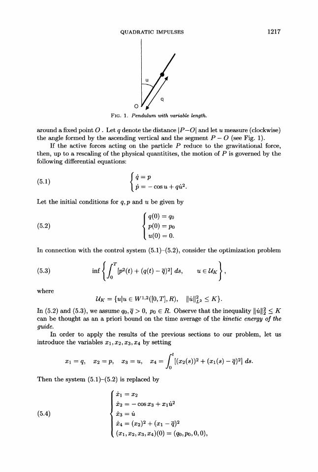
///FIG. 1. Pendulum with variable length.

around a fixed point O. Let q denote the distance IP-OI and let u measure (clockwise)the angle formed by the ascending vertical and the segment P- O (see Fig. 1).

If the active forces acting on the particle P reduce to the gravitational force,then, up to a rescaling of the physical quantitites, the motion of P is governed by thefollowing differential equations:

(5.1)p

ib cos u +Let the initial conditions for q, p and u be given by

q(0) q0

p(0) po0.

In connection with the control system (5.1)-(5.2), consider the optimization problem

{/0(5.3) inf [p(t) + (q(t) )2] ds, u e 14g

whereHK {UlU e W1,2([O, T], R), ]]itl]2L

_g}.

In (5.2) and (5.3), we assume q0, > 0, p0 R. Observe that the inequality II/tl122 _< Kcan be thought as an a priori bound on the time average of the kinetic energy of theguide.

In order to apply the results of the previous sections to our problem, let usintroduce the variables Xl, x2, x3, xa by setting

Xl q, X2 p, X3 U x4 [(x2(s))2 + (xl (s)- )2] ds.

Then the system (5.1)-(5.2) is replaced by


and our variational problem can be written as

(P) min{xa (T), u e

with UK C W1’2 as in 3. On the basis of the results of the previous sections we canassociate to (5.4) the impulsive system

where (v, w) e UK, also defined in 3.By the compactness of the set reachable by solutions of (5.5) (see Cor. 3.1), for

any K > 0 we obtain the existence of an optimal control pair for the extended problem

(P’) min {x4(T), (v, w) E g},where now x4(.) denotes the fourth component of the solution of (5.5). In order toexplicitly compute the optimal solution, when K is sufficiently large, we first writethe Euler necessary conditions for the variational problem

T(5.6) min [(q(t) )2 + O2(t)] dt, q(O) qo.

Solving the two-point boundary value problem

i(t) q(t) , q(O) qo, I(T) O,

one finds the unique optimal solution of (5.6)

-) cosh(t- T).q(t) + cosh(T)

Therefore, if K is sufficiently large and

(qo-)O(0+) \cs()sinh(-T) _> p0,

then the trajectory

( /o )(xl, x2, x3, x4)(t) q(t), (l(t), O, [(q(s) )2 + 02(s)] ds

is an optimal one for the generalized system (5.5).This trajectory corresponds to the control pair (v, w), with v(t) =_ O, w(O) 0

and

1 + /(s)(5.10) w(t) 4(0+)- Po + ds Vt > O.qo q(s)

QUADRATIC IMPULSESp

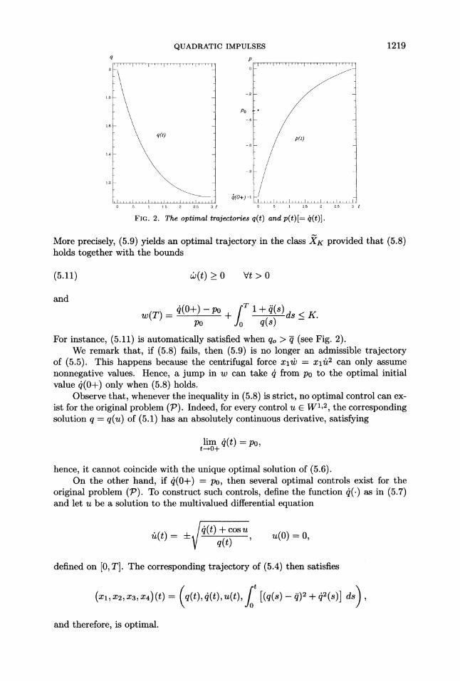
FIG. 2. The optimal trajectories q(t) and p(t)[= 0(t)].

1219

More precisely, (5.9) yields an optimal trajectory in the class XK provided that (5.8)holds together with the bounds

(5.11) &(t) >_ 0 Vt > 0

and

w(T) 0(0+) p0

p0

T 1 + q(s) ds < K.+ q(s)For instance, (5.11) is automatically satisfied when qo > (see Fig. 2).

We remark that, if (5.8) fails, then (5.9) is no longer an admissible trajectoryof (5.5). This happens because the centrifugal force xlb xl/t2 can only assumenonnegative values. Hence, a jump in w can take from p0 to the optimal initialvalue 4(0+) only when (5.8) holds.

Observe that, whenever the inequality in (5.8) is strict, no optimal control can ex-ist for the original problem (P). Indeed, for every control u E W1,2, the correspondingsolution q q(u) of (5.1) has an absolutely continuous derivative, satisfying

lim O(t) Po,t--,O+

hence, it cannot coincide with the unique optimal solution of (5.6).On the other hand, if (0+) p0, then several optimal controls exist for the

original problem (P). To construct such controls, define the function (.) as in (5.7)and let u be a solution to the multivalued differential equation

+I4(t) + cosq(t) u(O) =o,

defined on [0, T]. The corresponding trajectory of (5.4) then satisfies

( /0 )(Xl, X2, X3, X4)(t) q(t), O(t), u(t), [(q(s) 0)2 + 02(s)] ds

and therefore, is optimal.

1220 ALBERTO BRESSAN AND FRANCO I:tAMPAZZO

REFERENCES

[1] J. P. AUBIN AND A. CELLINA, Dijerential Inclusions, Springer, Berlin, 1984.[2] A. BRESSAN, On dierential systems with impulsive controls, Rend. Sem. Mat. Univ. Padova,

78 (1987), pp. 227-236.[3] A. BRESSAN AND V. RAMPAZZO, Impulsive control systems with commutative vector fields, J.

Optim. Theory Appl., 71 (1991), pp. 67-83.[4] Impulsive control systems without commutative assumptions, preprint 147M SISSA,

Trieste, Italy, 1990.[5] , On dierential systems with vector-valued impulsive controls. Bull. Univ. Mat. Ital.

B(7), 3 (1988), pp. 641-656.[6] A. BRESSAN, On control theory and its applications to certain problems for Lagrangian systems.

On hyperimpulsive motions for these (I, II). Atti Accad. Naz. Lincei Rend. CI. Sc. Fis.Mat. Natur. (8), 82 (1988), pp. 91-118.

[7] , On control theory and its applications to certain problems for Lagrangian systems. Onhyperimpulsive motions for these (III). Atti Accad. Naz. Lincei Rend. C1. Sci. Fis. Mat.Natur. (8), 82 (1988), pp. 461-471.

[8] , Hyperimpulsive motions and controllizable coordinates for Lagrangean systems. AttiAccad. Naz. Lincei Mem. C1. Sci. Fis. Mat. Natur. (8), 19 (1989).

[9] , On some control problem concerning the ski and the swing, Atti Accad. Naz. Lincei,Mem. C1. Sci. Fis. Mat. Natur. (9), 1 (1991), pp. 149-196., On some recent results in control theory, for their applications to Lagrangean systems,Atti Accad. Naz. Lincei Mem. C1. Sci. Fis. Mat. Natur. (8), 19 (1989).

H. BrtEZIS, Analyse fonctionnelle, Masson, Paris, 1987.G. DAL MASO AND F. RAMPAZZO, On systems of ordinary differential equations with measures

as controls, Differential and Integral Equations, 4 (1991), pp. 739-765.M. A. KRASNOSEL’SKII AND A. V. POKROVSKII, Vibrostable differential equations with a con-

tinuous right-hand side. Proc. Moscow Math. Soc., 27 (1972), pp. 93-113.F. RAMPAZZO, On Lagrangean systems with some coordinates as controls, Atti Accad. Naz.

Lincei Rend. C1. Sci. Fis. Mat. Natur., 82 (1988), pp. 685-695.., On the Riemannian structure of a Lagrangian system and the problem of adding time-dependent constraints as controls, European J. Mech. A Solids, 10 (1991), pp. 405-431., Optimal impulsive controls with a constraint on the total variation, in New Trends inSystems Theory, G. Conte, A. M. Perdon, B. F. Wyman, eds., Series Progress in Systemsand Control Theory, Birkhauser, Boston, 7 (1991), pp. 606-613.

A. V. SARYCHEV, Nonlinear systems with impulsive and generalized function controls, Proc.Conf. on Nonlinear Synthesis, Sopron, Hungary, 1989.

H. J. SUSSMANN, On the gap between deterministic and stochastic ordinary differential equa-tions, Ann. Probab., 6 (1978), pp. 17-41.

[10]

[11]

[13]

[14]

[15]

[16]

[17]

[18]

Reproducedwith permission of the copyright owner. Further reproduction prohibitedwithout permission.

on differential systems with quadratic impulses … · on differential systems with quadratic...

Documents