on correlations between ”dynamic” (small-strain) and ... · on correlations between...

On correlations between ”dynamic” (small-strain)and ”static” (large-strain) stiffness moduli

- an experimental investigation on 19 sands and gravels

T. Wichtmanni); I. Kimmigii); Th. Triantafyllidisiii)

NOTICE: This is the author’s version of a work that was accepted for publication in Soil Dynamics and Earthquake Engineering.Changes resulting from the publishing process, such as peer review, editing, corrections, structural formatting, and other qualitycontrol mechanisms may not be reflected in this document. Changes may have been made to this work since it was submitted forpublication. A definitive version was subsequently published in Soil Dynamics and Earthquake Engineering, Vol. 98, pp. 72-83, 2017,DOI: 10.1016/j.soildyn.2017.03.032

Abstract: Correlations between ”dynamic” (small-strain) and ”static” (large-strain) stiffness moduli for sand are exam-ined. Such correlations are often used for a simplified estimation of the dynamic stiffness based on static test data. Thesmall-strain shear modulus Gdyn = Gmax and the small-strain constrained modulus Mdyn = Mmax have been measured inresonant column (RC) tests with additional P-wave measurements. Oedometric compression tests were performed in orderto determine the large-strain constrained modulus Mstat = Moedo, while the large-strain Young’s modulus Estat = E50

was obtained from the initial stage of the stress-strain-curves measured in drained monotonic triaxial tests, evaluated as asecant stiffness between deviatoric stress q = 0 and q = qmax/2. Experimental data for 19 sands or gravels with speciallymixed grain size distribution curves, having different non-plastic fines contents, mean grain sizes and uniformity coefficients,were analyzed. Based on the present data, it is demonstrated that a correlation between Mmax and Moedo proposed inthe literature underestimates the dynamic stiffness of coarse and well-graded granular materials. Consequently, modifiedcorrelation diagrams for the relationship Mmax ↔ Moedo are proposed in the present paper. Furthermore, correlationsbetween Gmax and Moedo or E50, respectively, have been also investigated. They enable a direct estimation of dynamicshear modulus based on static test data. In contrast to the correlation diagram currently in use, the range of applicabilityof the new correlations proposed in this paper is clearly defined.

Keywords: Dynamic (small-strain) stiffness; Static (large-strain) stiffness; Correlations; Resonant column tests; P-wavemeasurements; Oedometric compression tests; Triaxial tests

1 IntroductionIt is well known that soil stiffness decreases with increas-ing magnitude of strain [1, 7, 8, 10, 14, 15, 20–22, 24–29,33–35, 37, 38, 43, 48, 49]. In many practical problems deal-ing with dynamic or cyclic loading (except soil liquefac-tion problems [18, 19, 23, 36]) the strain amplitudes gen-erated in the soil are relatively small. Furthermore, dy-namic measurement techniques like resonant column (RC)tests or wave propagation measurements are frequently ap-plied to determine the small-strain stiffness in the labora-tory [3,5–7,11,12,16,28,34,35,47]. Therefore, the stiffness atsmall strains is often also denoted as ”dynamic” stiffness.For the stiffness moduli applied in deformation (e.g. set-tlement) analysis of foundations, usually oedometric com-pression or triaxial tests with monotonic loading are con-ducted. The stiffness moduli resulting from these ”static”tests have been found significantly lower than the dynamicstiffness. Initially, this has been attributed to the differentloading rates applied in the static and dynamic tests. How-ever, it has been recognized soon that the material responseof sand is approximately rate-independent and that thosedifferences are due to the different strain levels.

i)Researcher, Institute of Soil Mechanics and Rock Mechanics,Karlsruhe Institute of Technology, Germany (corresponding author).Email: [email protected]

ii)Researcher, Institute of Soil Mechanics and Rock Mechanics,Karlsruhe Institute of Technology, Germanyiii)Professor and Director of the Institute of Soil Mechanics and Rock

Mechanics, Karlsruhe Institute of Technology, Germany

For the design of foundations subjected to dynamic load-ing, the small-strain shear modulus Gmax of the subsoil isa key parameter. For final design calculations in large orimportant projects it will be usually determined from dy-namic measurements in situ, e.g. surface or borehole mea-surements of the wave velocities. However, for feasibilitystudies, preliminary design calculations or final design cal-culations in small projects the small-strain shear modulusis often estimated from empirical formulas, tables or corre-lations with static stiffness values.

For design engineers in practice it is attractive to esti-mate the dynamic stiffness based on static stiffness data,because static tests are less elaborate than dynamic ones.While the dynamic experiments are conducted by special-ized laboratories only, even small soil mechanics laborato-ries are usually equipped with devices for oedometric test-ing. Furthermore, for many locations experienced data forthe static stiffness moduli are available. Without any fur-ther testing these data can be used to estimate the dynamicstiffness.

A diagram providing a correlation between static anddynamic stiffness moduli is incorporated e.g. in the ”Rec-ommendations of the working committee Soil Dynamics” ofthe German Geotechnical Society (DGGT) [9]. It is shownin Figure 1 (area marked by the dark gray colour). Thediagram is entered with the large-strain constrained mod-ulus Mstat = Moedo (stiffness on the primary compressionline obtained from oedometric compression tests) on the ab-

1

Wichtmann et al. Soil Dynamics and Earthquake Engineering, Vol. 98, pp. 72-83, 2017

scissa and delivers the ratio between small-strain and large-strain constrained moduli Mdyn/Mstat = Mmax/Moedo onthe ordinate. The small-strain shear modulus Gdyn =Gmax = Mmax(1 − ν − 2ν2)/[2(1 − ν)2] can be obtainedwith an assumption regarding Poisson’s ratio ν. Note, thatthe indices ⊔dyn and ⊔max are equivalent, i.e. both denotethe small-strain stiffness. The DGGT diagram is based onthe correlation between static and dynamic Young’s moduliproposed by Alpan [2]. This original correlation is also pre-sented in Figure 1 (black solid curve). Benz & Vermeer [4]have proposed another correlation between static and dy-namic constrained moduli (see the area marked by the lightgray colour in Figure 1). It is also based on Alpan [2], butin comparison to [9] different assumptions were used whenconverting the E data into a diagram in terms of M . How-ever, the experimental basis and the range of applicabilityof all correlations shown in Figure 1 is not clear [4, 45,46].

1 10 100 10001

2

5

10

20

50

100

Alpan (1970)

DGGT

Ed

yn/E

sta

t (c

urv

e o

f A

lpa

n)

Md

yn/M

sta

t (o

the

r cu

rve

s)

Estat [MPa] (curve of Alpan)

Mstat [MPa] (other curves)

Benz & Vermeer (2007)

Fig. 1: Correlation between Mdyn and Mstat according to the”Recommendations of the working committee Soil Dynamics”of the German Geotechnical Society (DGGT) [9] versus correla-tion proposed by Benz & Vermeer [4]. The original relationshipbetween Edyn and Estat according to Alpan [2] is also shown.

A first inspection of the correlations in Figure 1 for foursands with different grain size distribution curves has beenpresented in [44, 46]. It has been found that the dynamicstiffness of a coarse and a well-graded granular materialwas significantly underestimated by the range of the DGGTcorrelation. In consideration of the fact that this correlationis frequently used in practice (at least in Germany), it hasbeen decided to undertake a closer inspection, based onexperimental data collected for a wider range of grain sizedistribution curves. The present paper reports on that newstudy.

2 Tested materialsThe grain size distribution curves of the specially mixedsands or gravels tested in the present study are shown inFigure 2. These are the same mixtures that have been al-ready investigated in [39–43]. The raw material is a nat-ural fluvially deposited quartz sand obtained from a sandpit near Dorsten, Germany, which has been decomposedinto 25 gradations with grain sizes between 0.063 mm and16 mm. The grains have a subangular shape and the graindensity is ϱs = 2.65 g/cm3. The sands or gravels L1 to L8

(Figure 2a) have the same uniformity coefficient Cu = 1.5but different mean grain sizes in the range 0.1 mm ≤ d50 ≤6 mm. The materials L4 and L10 to L16 (Figure 2b) havethe same mean grain size d50 = 0.6 mm but different uni-formity coefficients 1.5 ≤ Cu ≤ 8. The inclination of thegrain size distribution curve of the fine sands F2 and F4 toF6 (Figure 2a) is similar to that of L1 (Cu = 1.5) but thesesands contain between 4.4 and 19.6 % silty fines (quartzpowder). The sands F1 and F3 have not been tested inthe present study but the numbering of the sands chosenin [39] has been maintained herein. The index properties ofall tested materials are summarized in Table 1.

L1 L2 L3 L4 L5 L6 L7

L4

L10L11

L12

L16

L15

L14

L13

0.06 0.2 0.6 2 60.02 200

20

40

60

80

100

SandSiltcoarse coarsefine finemedium medium

Gravel

Gravel

0

20

40

60

80

100

SandSiltcoarse coarsefine finemedium medium

Fin

er

by w

eig

ht [%

]

Grain size [mm]

0.06 0.2 0.6 2 60.02 20

Grain size [mm]

Fin

er

by w

eig

ht [%

]

a)

b)

F2F4F5F6

L8

Fig. 2: Tested grain size distribution curves

3 Small-strain stiffness from RC tests with addi-tional P-wave measurements

The small-strain stiffness moduli Gmax and Mmax were ob-tained from resonant column tests with additional P-wavemeasurements, using piezoelectric elements integrated intothe end plates of the RC device. The test device, the test-ing procedure and the test results are documented in detailin [39, 41–43]. The strain level associated with these mea-surements is about 10−6. For each sand, several samples(diameter d = 100 mm, height h = 200 mm) with differentinitial relative densities Dr0 = (emax − e0)/(emax − emin)were prepared by dry air pluviation and tested in the drycondition at various pressures. Figure 3 shows exemplarydata Gmax(e, p) and Mmax(e, p) for sand L12. Similar dia-grams for the other tested sands can be found in [41, 42].The increase of Gmax and Mmax with decreasing void ratioe and increasing mean pressure p is evident in Figure 3.In case of the coarsest tested material L8, Gmax(e, p) data

2


Mat. FC d50 Cu emin emax

[%] [mm] [-] [-] [-]

L1 0 0.1 1.5 0.634 1.127L2 0 0.2 1.5 0.596 0.994L3 0 0.35 1.5 0.591 0.931L4 0 0.6 1.5 0.571 0.891L5 0 1.1 1.5 0.580 0.879L6 0 2.0 1.5 0.591 0.877L7 0 3.5 1.5 0.626 0.817L8 0 6.0 1.5 0.634 0.799

L10 0 0.6 2 0.541 0.864L11 0 0.6 2.5 0.495 0.856L12 0 0.6 3 0.474 0.829L13 0 0.6 4 0.414 0.791L14 0 0.6 5 0.394 0.749L15 0 0.6 6 0.387 0.719L16 0 0.6 8 0.356 0.673

F2 4.4 0.092 1.5 0.734 1.107F4 11.3 0.086 1.9 0.726 1.117F5 14.0 0.084 2.6 0.723 1.174F6 19.6 0.082 3.3 0.746 1.091

Table 1: Index properties (non-plastic fines content FC, meangrain size d50, uniformity coefficient Cu = d60/d10, minimumand maximum void ratios emin, emax) of the tested granularmaterials.

are available, but P-wave measurements were not success-ful [42], i.e. no Mmax(e, p) data exist.

For each granular material, the data of the small-strainshear modulus Gmax(e, p) and the small-strain constrainedmodulus Mmax(e, p) have been approximated by the follow-ing equations going back to [13,16]:

Gmax = AGd(aGd − e)2

1 + e

(p

patm

)nGd

patm (1)

Mmax = AMd(aMd − e)2

1 + e

(p

patm

)nMd

patm (2)

with atmospheric pressure patm = 100 kPa. The optimumparameters AGd, aGd and nGd of Eq. (1) as well as AMd,aMd and nMd of Eq. (2) are collected in columns 2 - 7 ofTable 2. The notation of these parameters (and similar onesin the following) has been chosen in such way that the firstindex (G, M, E) denotes the type of stiffness and the secondone (d, s) stands for dynamic or static. The solid curves inFigure 3 represent the best fits of Eqs. (1) or (2) to thedata of each individual pressure, while the dashed curvesare generated using Eqs. (1) or (2) with the parametersgiven in columns 2 - 7 of Table 2.

In the RC tests, for constant values of void ratio andpressure, Gmax and Mmax were found to be rather inde-pendent of the mean grain size d50 of the test material (seeGmax data in Figure 4a,b). The only exception is the coars-est tested material L8, where the slightly lower Gmax valueswere presumably caused by an insufficient interlocking be-tween the grains and the end plates of the RC device [41].In contrast to the d50 independence, both small-strain stiff-ness values were significantly reduced when the uniformitycoefficient Cu and the content of non-plastic fines FC in-creased (Figure 4c-f). A micromechanical explanation ofthe observed trends of Gmax and Mmax with Cu and FCbased on contact stiffness [17,30] and force transition chainsin monodisperse and polydisperse materials [31, 32] is pro-

0.45 0.50 0.55 0.60 0.65 0.70 0.750

200

400

600

800

1000 Sand L12

d50 = 0.6 mm

Cu = 3

Constr

ain

ed m

odulu

s M

max [M

Pa]

Void ratio e [-]

Sand L12

0.500.45 0.55 0.60 0.65 0.70 0.750

50

100

150

200

250

300

Shear

modulu

s G

max [M

Pa]

Void ratio e [-]

p [kPa] =

50 200

75 300

100 400

150

p [kPa] =

50 200

75 300

100 400

150

d50 = 0.6 mm

Cu = 3

a)

b)

Fig. 3: a) Small strain shear modulus Gmax(e, p) and b) small-strain constrained modulus Mmax(e, p)measured in the RC testswith additional P-wave measurements on sand L12 (solid curves= best fit of Eqs. (1) or (2) to the data of the individual pres-sure steps, dashed curves = prediction of Eqs. (1) or (2) withparameters in columns 2 - 7 of Table 2)

vided in [39,41]. In [39,41,42] correlations of the parametersof Eqs. (1) or (2) with the granulometry have been pro-posed. They can be used for an estimation of small-strainstiffness considering the grain size distribution curve. Theestimation via static stiffness values described in this paperis an alternative.

4 Large-strain constrained modulus Moedo fromoedometric compression tests

All sands were tested in oedometric compression tests. Thesamples were prepared by air pluviation and tested in thedry condition. Different sample dimensions were used:

• Geometry I: diameter d = 100 mm, height h = 18 mm,d/h = 5.6 (used for tests on sands L1 - L3)

• Geometry II: d = 150 mm, h = 30 mm, d/h = 5.0(used for L1 - L6, L10 - L16, F2, F4 - F6)

• Geometry III: d = 280 mm, h = 80 mm, d/h = 3.8(used for L2 - L8, L10 - L16)

Most clean sands (L1 - L6, L10 - L16) were tested withtwo or three different specimen dimensions for comparisonpurpose. In the case of the largest tested geometry III twotests with loose and two other tests with dense specimens

3


Uniformity coefficient Cu = d60/d10

Fines content FC [%]

0.4 0.5 0.6 0.7 0.8

Void ratio e

Void ratio e

0.70 0.75 0.80 0.85 0.90 0.95

1 2 3 4 5 6 7 8 9

0

40

80

120

160

0.5 0.6 0.7 0.8 0.90

50

100

150

200

250

300S

he

ar

mo

du

lus G

ma

x [

MP

a]

Void ratio e

p = 400 kPa

a)

c)

e) f)

p = 400 kPa

L4 / 1.5L10 / 2L12 / 3L14 / 5L16 / 8

Sand / Cu =

d)

p [kPa] =

50100

200

400

e = 0.55

0

50

100

150

200

Mean grain size d50 [mm]

0.1 0.2 0.5 1 2 5 10

b)

0

50

100

150

200

250

300

Sh

ear

mo

du

lus G

ma

x [

MP

a]

0

50

100

150

200

250

300

Shea

r m

od

ulu

s G

ma

x [M

Pa

]

0

50

100

150

200

250

300

She

ar

mod

ulu

s G

ma

x [M

Pa

]S

he

ar

mo

dulu

s G

ma

x [

MP

a]

She

ar

mod

ulu

s G

ma

x [

MP

a]

Sand /

FC [%] =

L1 / 0

F4 / 11.3

F5 / 14.0F2 / 4.4 F6 / 19.6

p = 400 kPa

0 5 10 15 20 25

p [kPa] =

50100

200

400e = 0.825

p [kPa] =

50100

200

400e = 0.70

Sand / d50 [mm] =

L1 / 0.1L2 / 0.2L3 / 0.35L4 / 0.6

L5 / 1.1L6 / 2.0L7 / 3.5L8 / 6.0

Fig. 4: Small-strain shear modulus Gmax from resonant column tests a,b) does not depend on mean grain size d50 but decreases withc,d) uniformity coefficient Cu and e,f) fines content FC (adapted from [39,41,42])

have been performed. In the tests with both smaller sam-ple geometries I and II several samples with various initialdensities between loose and dense were tested. Owed to dif-ferent loading devices the maximum axial stress was σmax

1 ≈900 kPa in the case of geometry I, 400 kPa for II and 800kPa for III.

In each oedometric compression test the axial load hasbeen increased to the maximum vertical stress σmax

1 , fol-lowed by an unloading to σ1 = 0 and a final reloading toσmax1 . Typical curves of void ratio or axial strain versus ax-

ial stress from tests with geometry III are given in Figure5. The constrained modulus Moedo has been derived fromthe compression curve measured during the first loading to

σmax1 . The un- and reloading curves are not further used in

this paper. Moedo is calculated with the increments of axialstress ∆σ1 and void ratio ∆e and with the void ratio e0 atthe beginning of a load step:

Moedo =∆σ1

∆ε1=

∆σ1

∆e(1 + e0) (3)

Alternatively, it can be obtained from Moedo = [ln(10)(1 +e0)σ1]/Cc with Cc being the actual inclination of the com-pression curve in a e-log σ1 diagram at the actual axialstress σ1. The stiffness Moedo has been evaluated for thesame values of mean pressure p = (σ1 + 2σ3)/3 that havebeen used in the RC tests (p = 50, 75, 100, 150, 200 and

4


1 2 3 4 5 6 7 8 9 10 11 12 13 14Mat. Gmax, Eq. (1) Mmax, Eq. (2) Moedo, Eqs. (4) + (5) E50, Eq. (6)

AGd aGd nGd AMd aMd nMd AMs a1,Ms a2,Ms nMs AEs aEs nEs

L1 636 2.34 0.44 547 3.73 0.38 2860 1.37 0.000 0.66 – – –L2 1521 1.79 0.43 3657 1.98 0.37 2320 1.45 0.035 0.59 7500 0.95 0.70L3 1620 1.77 0.42 3172 2.11 0.35 660 1.90 0.045 0.59 4500 0.95 0.70L4 2023 1.67 0.41 5804 1.76 0.34 640 1.98 0.080 0.76 5400 0.91 1.00L5 1570 1.77 0.43 3319 2.05 0.37 1150 1.80 0.100 0.84 4200 0.94 0.88L6 1035 2.04 0.43 3151 2.10 0.40 300 2.63 0.160 0.81 1000 1.20 0.90L7 852 2.13 0.45 620 3.80 0.41 850 1.90 0.105 0.80 – – –L8 734 2.16 0.45 – – – 350 2.62 0.160 0.75 – – –

L10 1207 1.85 0.46 2679 2.20 0.36 1270 1.65 0.075 0.72 – – –L11 2240 1.47 0.48 3280 2.04 0.37 600 1.99 0.100 0.76 – – –L12 2489 1.39 0.50 5512 1.69 0.37 750 1.88 0.110 0.85 5600 0.78 1.00L13 2969 1.27 0.51 9363 1.40 0.38 730 1.84 0.135 1.06 – – –L14 2771 1.26 0.54 4789 1.72 0.40 470 1.98 0.100 0.86 8000 0.69 0.70L15 4489 1.08 0.53 10366 1.30 0.40 700 1.76 0.090 0.82 – – –L16 2388 1.27 0.54 17286 1.08 0.42 880 1.54 0.065 0.79 5200 0.68 0.57

F2 571 2.19 0.51 14.7 16.3 0.44 3138 1.32 0.000 0.69 – – –F4 81.6 3.83 0.58 127.7 5.58 0.48 2206 1.32 0.000 0.69 1600 1.13 0.95F5 71.5 4.09 0.57 170.4 4.97 0.48 1717 1.32 0.000 0.72 – – –F6 17.9 7.19 0.57 132.2 5.39 0.49 2253 1.29 0.000 0.70 2270 1.06 0.84

Table 2: Parameters of Eqs. (1), (2), (4), (5) and (6) for all tested materials

300 kPa). Since the lateral stress could not be measuredin the oedometric compression tests, it has been estimatedfrom σ3 = K0σ1 with K0 = 1 − sinφP . The peak frictionangle φP has been obtained from the drained monotonictriaxial tests (Section 5). Due to the limitations in σmax

1 , amean pressure of p = 400 kPa that was applied in the RCtests was not reached in the oedometric compression tests.For d = 100 and 280 mm, the attainable pressure was re-stricted to p = 300 kPa, while it was p = 200 kPa or evenonly 150 kPa for d = 150 mm (depending on density viaφP (Dr)). The axial strains corresponding to the evaluatedMoedo values ranged from ε1 = 0.24 % for the dense sampleof L8 at p = 50 kPa to ε1 = 5.6 % for the loose sample ofF5 at p = 150 kPa (compare also data for L3 in Figure 5b).Therefore, the strains in the oedometric compression testsare about 2,000 to 50,000 times larger than those in themeasurements of the small-strain stiffness.

The smallest tested sample geometry (d = 100 mm, h =18 mm) was found inappropriate since even for fine sands itdelivered significantly lower Moedo values than both othersample dimensions (d = 150 mm, h = 30 mm and d = 280mm, h = 80 mm, see data for L1 and L2 in Figure 6a,b). Foruniform fine to medium coarse sands (d50 ≤ 2 mm, Cu ≤2.5) oedometric compression tests with d = 150 mm, h = 30mm seem to deliver acceptable results since similar stiffnessvalues as for d = 280 mm, h = 80 mm were obtained (seedata for L2 and L11 in Figure 6b,d). For coarse and well-graded granular materials the largest sample geometry wasnecessary to collect reliable Moedo data, since the stiffnessvalues for d = 150 mm, h = 30 mm were found lower thanfor d = 280 mm, h = 80 mm (see data for L5, L13 and L15in Figure 6c,e,f).

The weaker response of the smaller samples probably re-sults from a loosened layer at the top originating from thesample preparation process. The alignment of the upperlayer of grains to the load piston during the initial phase ofloading may also have contributed to the weaker response.Both influences are larger in case of the samples with lower

10 100 10000.84

0.86

0.92

0.94

Void

ratio e

Axial stress σ1 [kPa]

1

0.88

0.90

First loading

Unloading

Reloading

10 100 10003.0

2.5

1.0

0.0Dr0 = 0.93

Dr0 = 0.03

Dr0 = 0.03

Axia

l str

ain

ε1 [

%]

Axial stress σ1 [kPa]

1

2.0

1.5

0.5

a)

b)

Fig. 5: a) Void ratio and b) axial strain ε1 versus axial stress inoedometric compression tests on sand L3

5


0.6 0.7 0.8 0.9 1.0 1.10

30

60

90

120

150

180

0.5 0.6 0.7 0.8 0.9 1.0 0.5 0.6 0.7 0.8 0.9 1.0

0.4 0.5 0.6 0.7 0.8 0.9 1.0 0.4 0.5 0.6 0.7 0.8 0.9 0.3 0.4 0.5 0.6 0.7 0.8 0.9

L1 L2 L5

L15L13L11

Stiffness M

oe

do [M

Pa]

Void ratio e

Void ratio e Void ratio e Void ratio e

Void ratio e Void ratio e

Sample geometry:

d [mm] / h [mm]

I: 100 / 18II: 150 / 30

Sample geometry:

d [mm] / h [mm]

I: 100 / 18

II: 150 / 30

III: 280 / 80

a)

0

30

60

90

120

150

180

Stiffness M

oe

do [M

Pa]

b)

0

30

60

90

120

150

180

Stiffness M

oe

do [M

Pa]

c)

0

30

60

90

120

150

180

Stiffness M

oe

do [M

Pa]

d)

0

30

60

90

120

150

180

Stiffness M

oe

do [M

Pa]

e)

0

30

60

90

120

150

180

Stiffness M

oe

do [M

Pa]

f)

Sample geometry:

d [mm] / h [mm]

II: 150 / 30

III: 280 / 80

Sample geometry:

d [mm] / h [mm]

II: 150 / 30

III: 280 / 80

Sample geometry:

d [mm] / h [mm]

II: 150 / 30

III: 280 / 80

Sample geometry:

d [mm] / h [mm]

II: 150 / 30

III: 280 / 80

Fig. 6: Comparison of Moedo(e) data for p = 150 kPa obtained from oedometric compression tests with different sample geometries

0.6 0.7 0.8 0.9 1.0 1.10

30

60

90

120

150

180

0.5 0.6 0.7 0.8 0.9 1.0 0.5 0.6 0.7 0.8 0.9 1.0

0.4 0.5 0.6 0.7 0.8 0.9 1.0 0.3 0.4 0.5 0.6 0.7 0.8 0.6 0.7 0.8 0.9 1.0

p [kPa] =

5075100

150200

p [kPa] =

5075100

150200

p [kPa] =

5075100

150200300

p [kPa] =

5075100

150200300

p [kPa] =

5075100

150200300

p [kPa] =

5075100

150200300

L1

L12 L16 F6

L4 L7

Stiffness M

oe

do [M

Pa]


Void ratio eVoid ratio eVoid ratio e

a)

0

30

60

90

120

150

180

Stiffness M

oe

do [M

Pa]

b)

0

30

60

90

120

150

180

Stiffness M

oe

do [M

Pa]

c)

0

30

60

90

120

150

180

Stiffness M

oe

do [M

Pa]

d)

0

30

60

90

120

150

180

Stiffness M

oe

do [M

Pa]

e)

0

30

60

90

120

150

180

Stiffness M

oe

do [M

Pa]

f)

Fig. 7: Moedo(e, p) data for selected sands, obtained from the oedometric compression tests with the largest tested sample geometry.The black solid curves have been generated using Eqs. (4) and (5) with the parameters given in columns 8 - 11 of Table 2.

height and become more pronounced if the grain size in-creases. In contrast, side friction effects seem to be of mi-nor importance. All three tested sample dimensions are inaccordance with German standard code DIN 18135 for oe-dometric testing (d/h ≥ 3). The ratio of the contact areabetween the soil and the side wall Awall and the area ofthe sample cross section Asample increases with increasingsample size. It is Awall/Asample = 0.72 for d = 100 mm,0.80 for d = 150 mm and 1.14 for d = 280 mm. There-fore, the side friction effects will slightly increase with thesample size. The influence on the test data seems, how-ever, to be relatively small since for finer sands (e.g. L2

and L11 in Figure 6) quite similar stiffness values were ob-tained from the tests with d = 150 mm and d = 280 mm.Furthermore, if side friction effects were the main reasonfor the observed geometry influence, then the differences inthe stiffness moduli obtained for the different sample ge-ometries should be almost the same for all sands, i.e. thegeometry effects should not depend on grain size distribu-tion curve. This is contrasted by the current experimentalresults.

For the analysis of the correlations with small-strain stiff-ness values in Section 6, theMoedo data of the largest testedgeometry were selected for each sand, i.e. geometry II for

6


0.4 0.5 0.6 0.7 0.8 0.9 1.0 1.10

20

40

60

80

100

120

0.4 0.5 0.6 0.7 0.8 0.9 1.0 1.10

40

80

120

160

200

0.4 0.5 0.6 0.7 0.8 0.9 1.0 1.10

40

80

120

160

200

240

0.3 0.4 0.5 0.6 0.7 0.8 0.9 1.00

20

40

60

80

100

0.3 0.4 0.5 0.6 0.7 0.8 0.9 1.00

40

80

120

160

200

240

0.3 0.4 0.5 0.6 0.7 0.8 0.9 1.00

40

80

120

160

200

240

0.6 0.7 0.8 0.9 1.0 1.10

20

40

60

80

0.6 0.7 0.8 0.9 1.0 1.10

20

40

60

80

100

120

140

Void ratio e

Stiff

ne

ss M

oe

do [

MP

a]

Stiff

ne

ss M

oe

do [

MP

a]

Stiff

ne

ss M

oe

do [

MP

a]

Stiff

ne

ss M

oe

do [

MP

a]

Stiff

ne

ss M

oe

do [

MP

a]

Stiff

ne

ss M

oe

do [

MP

a]

Stiff

ne

ss M

oe

do [

MP

a]

Stiff

ne

ss M

oe

do [

MP

a]




p = 50 kPa p = 150 kPa

p = 50 kPa p = 150 kPa p = 300 kPa

p = 50 kPa p = 150 kPa p = 300 kPa

L4 / 1.5

Sand / Cu =

L10 / 2.0L11 / 2.5L12 / 3.0L13 / 4.0L14 / 5.0L15 / 6.0L16 / 8.0

L1 / 0

Sand /

FC [%] =

F2 / 4.4F4 / 11.3F5 / 14.0F6 / 19.6

L1 / 0

Sand /

FC [%] =

F2 / 4.4F4 / 11.3F5 / 14.0F6 / 19.6

L4 / 1.5

Sand / Cu =

L10 / 2.0L11 / 2.5L12 / 3.0L13 / 4.0L14 / 5.0L15 / 6.0L16 / 8.0

L4 / 1.5

Sand / Cu =

L10 / 2.0L11 / 2.5L12 / 3.0L13 / 4.0L14 / 5.0L15 / 6.0L16 / 8.0

a) b) c)

d) e) f)

g) h)

L1 / 0.1

Sand /

d50 [mm] =

L2 / 0.2L3 / 0.35L4 / 0.6L5 / 1.0L6 / 2.0L7 / 3.5L8 / 6.0

L1 / 0.1

Sand /

d50 [mm] =

L2 / 0.2L3 / 0.35L4 / 0.6L5 / 1.0L6 / 2.0L7 / 3.5L8 / 6.0

L1 / 0.1

Sand /

d50 [mm] =

L2 / 0.2L3 / 0.35L4 / 0.6L5 / 1.0L6 / 2.0L7 / 3.5L8 / 6.0

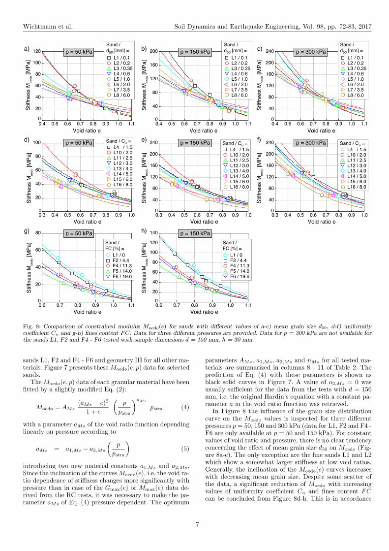
Fig. 8: Comparison of constrained modulus Moedo(e) for sands with different values of a-c) mean grain size d50, d-f) uniformitycoefficient Cu and g-h) fines content FC. Data for three different pressures are provided. Data for p = 300 kPa are not available forthe sands L1, F2 and F4 - F6 tested with sample dimensions d = 150 mm, h = 30 mm.

sands L1, F2 and F4 - F6 and geometry III for all other ma-terials. Figure 7 presents these Moedo(e, p) data for selectedsands.

TheMoedo(e, p) data of each granular material have beenfitted by a slightly modified Eq. (2):

Moedo = AMs(aMs − e)2

1 + e

(p

patm

)nMs

patm (4)

with a parameter aMs of the void ratio function dependinglinearly on pressure according to

aMs = a1,Ms − a2,Ms

(p

patm

)(5)

introducing two new material constants a1,Ms and a2,Ms.Since the inclination of the curvesMoedo(e), i.e. the void ra-tio dependence of stiffness changes more significantly withpressure than in case of the Gmax(e) or Mmax(e) data de-rived from the RC tests, it was necessary to make the pa-rameter aMs of Eq. (4) pressure-dependent. The optimum

parameters AMs, a1,Ms, a2,Ms and nMs for all tested ma-terials are summarized in columns 8 - 11 of Table 2. Theprediction of Eq. (4) with these parameters is shown asblack solid curves in Figure 7. A value of a2,Ms = 0 wasusually sufficient for the data from the tests with d = 150mm, i.e. the original Hardin’s equation with a constant pa-rameter a in the void ratio function was retrieved.

In Figure 8 the influence of the grain size distributioncurve on the Moedo values is inspected for three differentpressures p = 50, 150 and 300 kPa (data for L1, F2 and F4 -F6 are only available at p = 50 and 150 kPa). For constantvalues of void ratio and pressure, there is no clear tendencyconcerning the effect of mean grain size d50 on Moedo (Fig-ure 8a-c). The only exception are the fine sands L1 and L2which show a somewhat larger stiffness at low void ratios.Generally, the inclination of the Moedo(e) curves increaseswith decreasing mean grain size. Despite some scatter ofthe data, a significant reduction of Moedo with increasingvalues of uniformity coefficient Cu and fines content FCcan be concluded from Figure 8d-h. This is in accordance

7


with the tendencies measured for the small-strain stiffnessmoduli Gmax and Mmax in the RC tests (Figure 4c-f).

5 Large-strain Young’s modulus E50 from drainedmonotonic triaxial tests

Young’s modulus E50 is obtained from the initial stage ofthe stress-strain curve measured in drained monotonic tri-axial tests. It is evaluated as a secant stiffness for the in-terval between deviatoric stress q = 0 and q = qmax/2.For all tested materials several drained monotonic triaxialtests with a variation of initial relative density were per-formed. The effective lateral stress was σ′

3 = 100 kPa inall these tests. All samples (d = 100 mm, h = 100 mm)were prepared by air pluviation and afterwards saturatedwith de-aired water. Based on the data of these tests thedensity-dependent peak friction angle φP (Dr) used in orderto estimate the lateral stress in the oedometric compres-sion tests (see Section 4) has been evaluated. In additionaltests on medium dense samples, ten sands (L2 - L6, L12,L14, L16, F4, F6) were also sheared under higher confiningstresses σ′

3 = 200 and 400 kPa. Since tests with differentconfining stresses are necessary to quantify the pressure-dependence of stiffness, only these ten sands are analyzedin the following with respect to E50(e, p). Figure 9 showstypical curves of deviatoric stress q versus axial strain ε1measured in two tests with different initial relative densities(Dr0 = 0.51 or 0.87) performed on sand L4. The determi-nation of Young’s modulus E50 = ∆σ1/∆ε1 = ∆q/∆ε1from the initial part of the stress-strain curve is also illus-trated in Figure 9. The axial strains corresponding to theevaluated E50 values ranged from ε1 = 0.5 % for the densesample of L4 at σ′

3 = 100 kPa to ε1 = 2.3 % for the loosesample of L1 at σ′

3 = 100 kPa, being about 5,000 to 20,000times larger than those corresponding to the small-strainstiffness.

0 3 6 9 12 15 180

75

150

225

300

375

450

Devia

toric s

tress q

[kP

a]

Axial strain ε1 [%]

qpeak,2

= 381.8

ε1 (q

50,2 )

E50,1

E50,2

100 / 0.87

1 100 / 0.51

2

σ3’ [kPa] / D

r0 =

qpeak,1

= 291.7

q50,2 = 190.9

q50,1

= 145.9

ε1 (q

50,1 )

1

1

1

2

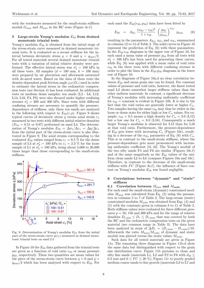
Fig. 9: Determination of Young’s modulus E50 from the initialpart of the stress-strain curve q(ε1) measured in drained mono-tonic triaxial tests on sand L4

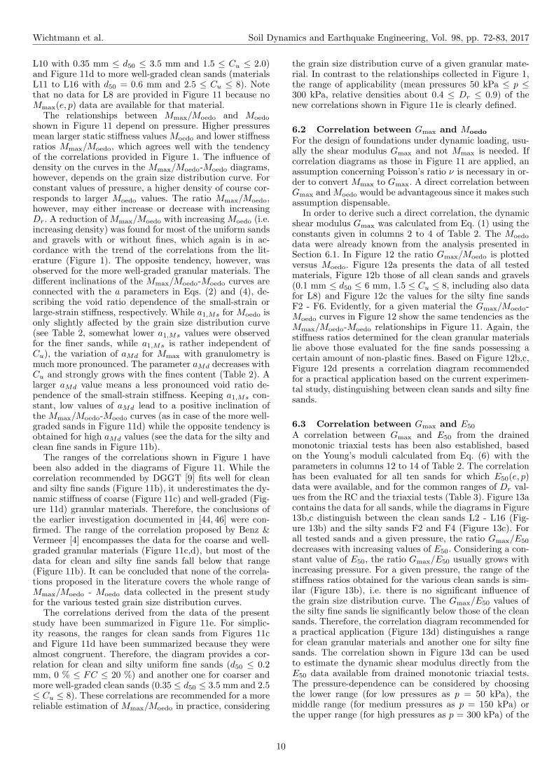
In Figure 10 the E50 data gathered from the triaxial testsare given as a function of void ratio e50 or mean pressurep50, respectively. These two quantities are mean values forthe piece of the stress-strain curve between q = 0 and q =qmax/2 which has been analyzed with respect to E50. For

each sand the E50(e50, p50) data have been fitted by

E50 = AEs(aEs − e50)

2

1 + e50

(p50patm

)nEs

patm (6)

resulting in the parameters AEs, aEs and nEs summarizedin columns 12 to 14 of Table 2. The solid curves in Figure 10represent the prediction of Eq. (6) with these parameters.In the E50-e50 diagrams in the upper row of Figure 10, foreach sand a mean value of pressure p50 from all tests withσ′3 = 100 kPa has been used for generating these curves,

while Eq. (6) was applied with a mean value of void ratioe50 in the three tests with different confining stresses inorder to plot the lines in the E50-p50 diagrams in the lowerrow of Figure 10.

In the diagrams of Figure 10a,d no clear correlation be-tween E50 and mean grain size can be found. For constantvalues of pressure and void ratio, however, the finest testedsand L2 shows somewhat larger stiffness values than theother uniform materials. In contrast, a significant decreaseof Young’s modulus with increasing uniformity coefficientfor e50 = constant is evident in Figure 10b. It is due to thefact that the void ratios are generally lower at higher Cu.Two samples having the same e50 may thus be either in theloose or dense state for either high or low Cu values. For ex-ample, e50 = 0.5 means a high density for Cu = 3.0 (L12)but a low one for Cu = 8.0 (L16). Consequently a muchlarger Young’s modulus is observed for L12 than for L16at that void ratio. Furthermore, the pressure-dependenceof E50 gets lower with increasing Cu (Figure 10e), result-ing in a decrease of the nEs parameter of Eq. (6) with Cu.This is in contrast to the small-strain stiffness, where thepressure-dependence gets more pronounced with increas-ing uniformity coefficient [41, 42]. The Young’s moduli ofthe two silty sands F4 and F6 are similar (Figures 10c,f)and of the same magnitude as the E50 values of the uni-form clean sands L2 to L6 (compare Figures 10a and 10c).Therefore, in contrast to the decrease of the small-strainstiffness with FC (Figure 3e,f), the influence of fines con-tent on Young’s modulus E50 was found negligible.

6 Correlations between ”dynamic” and ”static”stiffness

6.1 Correlation between Mmax and Moedo

For each sand the small-strain (dynamic) constrained mod-ulus Mmax was calculated from Eq. (2) using the parame-ters in columns 5 to 7 of Table 2. The large-strain (static)constrained modulus Moedo was obtained from Eqs. (4) and(5) with the constants given in columns 8 to 11 of Table 2.Both stiffness values were evaluated for three different pres-sures p = 50, 150 and 300 kPa and for the range of relativedensities Dr,min ≤ Dr ≤ Dr,max that was covered by boththe RC and the oedometric compression tests on the givenmaterial (see common range in Table 3). The data havebeen analyzed in steps of ∆Dr = (Dr,max − Dr,min)/10.Afterwards the ratio Mmax/Moedo of dynamic and staticmoduli was plotted versus the static values Moedo.

Such data for all tested materials are given in Figure11a. The remaining three diagrams in Figure 11b-d showthe same data but distinguished with respect to the grainsize distribution curve. Figure 11b pertains to clean andsilty fine sands (materials L1, L2 and F2 to F6 with d50 ≤0.2 mm and 0 ≤ FC ≤ 20 %), Figure 11c to poorly gradedmedium coarse sands to fine gravels (materials L3 to L7 and

8


0.3 0.4 0.5 0.6 0.7 0.8 0.9 1.00

10

20

30

40

50

60

0.3 0.4 0.5 0.6 0.7 0.8 0.9 1.0

50 100 200 500 10001

5

10

20

50

100

200

400 Y

ou

ng

’s m

od

ulu

s E

50 [

MP

a]

Yo

un

g’s

mo

du

lus E

50 [

MP

a]

Void ratio e50 Void ratio e50

Mean pressure p50 [kPa]

L2 / 0.2

L6 / 2.0

L4 / 0.6

L5 / 1.0

L3 / 0.35

Sand/d

50 [mm] =

L2 / 0.2

L6 / 2.0

L4 / 0.6

L5 / 1.0

L3 / 0.35

Sand/d

50 [mm] =

Sand / Cu =

L4 / 1.5

L14 / 5.0

L16 / 8.0

L12 / 3.0

Sand / FC [%] =

F4 / 11.3

F6 / 19.6

Sand / FC [%] =

F4 / 11.3

F6 / 19.6

0

10

20

30

40

50

60

Yo

un

g’s

mo

du

lus E

50 [

MP

a]

0

10

20

30

40

50

60

Yo

un

g’s

mo

du

lus E

50 [

MP

a]

0.3 0.4 0.5 0.6 0.7 0.8 0.9 1.0

Void ratio e50

σ3' = 100 kPa σ3' = 100 kPa

σ3' = 100 kPa

50 100 200 500 10001

5

10

20

50

100

200

400 Y

ou

ng

’s m

od

ulu

s E

50 [

MP

a]


50 100 200 500 10001

5

10

20

50

100

200

400 Y

ou

ng

’s m

od

ulu

s E

50 [

MP

a]


a) b) c)

d) e) f)

Sand / Cu =

L4 / 1.5

L14 / 5.0

L16 / 8.0

L12 / 3.0

Fig. 10: Young’s modulus E50 derived from the drained monotonic triaxial tests as a function of void ratio e50 (upper row, for σ′3

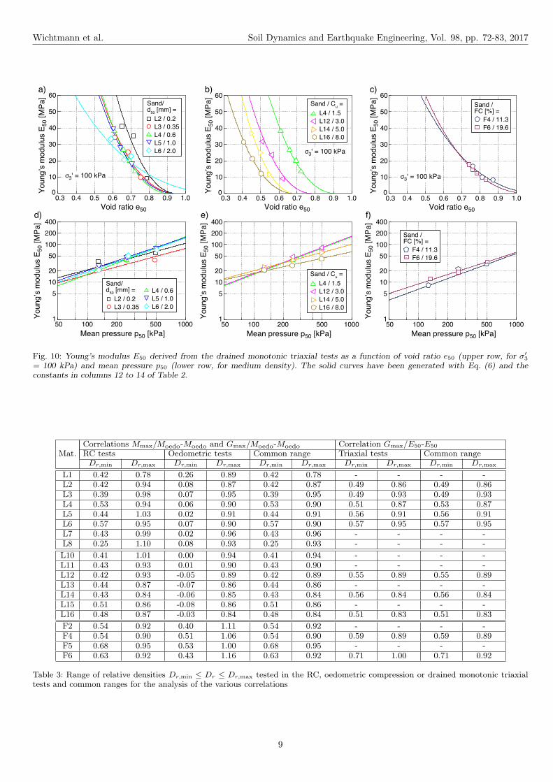
= 100 kPa) and mean pressure p50 (lower row, for medium density). The solid curves have been generated with Eq. (6) and theconstants in columns 12 to 14 of Table 2.

Correlations Mmax/Moedo-Moedo and Gmax/Moedo-Moedo Correlation Gmax/E50-E50

Mat. RC tests Oedometric tests Common range Triaxial tests Common rangeDr,min Dr,max Dr,min Dr,max Dr,min Dr,max Dr,min Dr,max Dr,min Dr,max

L1 0.42 0.78 0.26 0.89 0.42 0.78 - - - -L2 0.42 0.94 0.08 0.87 0.42 0.87 0.49 0.86 0.49 0.86L3 0.39 0.98 0.07 0.95 0.39 0.95 0.49 0.93 0.49 0.93L4 0.53 0.94 0.06 0.90 0.53 0.90 0.51 0.87 0.53 0.87L5 0.44 1.03 0.02 0.91 0.44 0.91 0.56 0.91 0.56 0.91L6 0.57 0.95 0.07 0.90 0.57 0.90 0.57 0.95 0.57 0.95L7 0.43 0.99 0.02 0.96 0.43 0.96 - - - -L8 0.25 1.10 0.08 0.93 0.25 0.93 - - - -

L10 0.41 1.01 0.00 0.94 0.41 0.94 - - - -L11 0.43 0.93 0.01 0.90 0.43 0.90 - - - -L12 0.42 0.93 -0.05 0.89 0.42 0.89 0.55 0.89 0.55 0.89L13 0.44 0.87 -0.07 0.86 0.44 0.86 - - - -L14 0.43 0.84 -0.06 0.85 0.43 0.84 0.56 0.84 0.56 0.84L15 0.51 0.86 -0.08 0.86 0.51 0.86 - - - -L16 0.48 0.87 -0.03 0.84 0.48 0.84 0.51 0.83 0.51 0.83

F2 0.54 0.92 0.40 1.11 0.54 0.92 - - - -F4 0.54 0.90 0.51 1.06 0.54 0.90 0.59 0.89 0.59 0.89F5 0.68 0.95 0.53 1.00 0.68 0.95 - - - -F6 0.63 0.92 0.43 1.16 0.63 0.92 0.71 1.00 0.71 0.92

Table 3: Range of relative densities Dr,min ≤ Dr ≤ Dr,max tested in the RC, oedometric compression or drained monotonic triaxialtests and common ranges for the analysis of the various correlations

9


L10 with 0.35 mm ≤ d50 ≤ 3.5 mm and 1.5 ≤ Cu ≤ 2.0)and Figure 11d to more well-graded clean sands (materialsL11 to L16 with d50 = 0.6 mm and 2.5 ≤ Cu ≤ 8). Notethat no data for L8 are provided in Figure 11 because noMmax(e, p) data are available for that material.

The relationships between Mmax/Moedo and Moedo

shown in Figure 11 depend on pressure. Higher pressuresmean larger static stiffness values Moedo and lower stiffnessratios Mmax/Moedo, which agrees well with the tendencyof the correlations provided in Figure 1. The influence ofdensity on the curves in the Mmax/Moedo-Moedo diagrams,however, depends on the grain size distribution curve. Forconstant values of pressure, a higher density of course cor-responds to larger Moedo values. The ratio Mmax/Moedo,however, may either increase or decrease with increasingDr. A reduction of Mmax/Moedo with increasing Moedo (i.e.increasing density) was found for most of the uniform sandsand gravels with or without fines, which again is in ac-cordance with the trend of the correlations from the lit-erature (Figure 1). The opposite tendency, however, wasobserved for the more well-graded granular materials. Thedifferent inclinations of the Mmax/Moedo-Moedo curves areconnected with the a parameters in Eqs. (2) and (4), de-scribing the void ratio dependence of the small-strain orlarge-strain stiffness, respectively. While a1,Ms for Moedo isonly slightly affected by the grain size distribution curve(see Table 2, somewhat lower a1,Ms values were observedfor the finer sands, while a1,Ms is rather independent ofCu), the variation of aMd for Mmax with granulometry ismuch more pronounced. The parameter aMd decreases withCu and strongly grows with the fines content (Table 2). Alarger aMd value means a less pronounced void ratio de-pendence of the small-strain stiffness. Keeping a1,Ms con-stant, low values of aMd lead to a positive inclination ofthe Mmax/Moedo-Moedo curves (as in case of the more well-graded sands in Figure 11d) while the opposite tendency isobtained for high aMd values (see the data for the silty andclean fine sands in Figure 11b).

The ranges of the correlations shown in Figure 1 havebeen also added in the diagrams of Figure 11. While thecorrelation recommended by DGGT [9] fits well for cleanand silty fine sands (Figure 11b), it underestimates the dy-namic stiffness of coarse (Figure 11c) and well-graded (Fig-ure 11d) granular materials. Therefore, the conclusions ofthe earlier investigation documented in [44, 46] were con-firmed. The range of the correlation proposed by Benz &Vermeer [4] encompasses the data for the coarse and well-graded granular materials (Figure 11c,d), but most of thedata for clean and silty fine sands fall below that range(Figure 11b). It can be concluded that none of the correla-tions proposed in the literature covers the whole range ofMmax/Moedo - Moedo data collected in the present studyfor the various tested grain size distribution curves.

The correlations derived from the data of the presentstudy have been summarized in Figure 11e. For simplic-ity reasons, the ranges for clean sands from Figures 11cand Figure 11d have been summarized because they werealmost congruent. Therefore, the diagram provides a cor-relation for clean and silty uniform fine sands (d50 ≤ 0.2mm, 0 % ≤ FC ≤ 20 %) and another one for coarser andmore well-graded clean sands (0.35 ≤ d50 ≤ 3.5 mm and 2.5≤ Cu ≤ 8). These correlations are recommended for a morereliable estimation of Mmax/Moedo in practice, considering

the grain size distribution curve of a given granular mate-rial. In contrast to the relationships collected in Figure 1,the range of applicability (mean pressures 50 kPa ≤ p ≤300 kPa, relative densities about 0.4 ≤ Dr ≤ 0.9) of thenew correlations shown in Figure 11e is clearly defined.

6.2 Correlation between Gmax and Moedo

For the design of foundations under dynamic loading, usu-ally the shear modulus Gmax and not Mmax is needed. Ifcorrelation diagrams as those in Figure 11 are applied, anassumption concerning Poisson’s ratio ν is necessary in or-der to convert Mmax to Gmax. A direct correlation betweenGmax andMoedo would be advantageous since it makes suchassumption dispensable.

In order to derive such a direct correlation, the dynamicshear modulus Gmax was calculated from Eq. (1) using theconstants given in columns 2 to 4 of Table 2. The Moedo

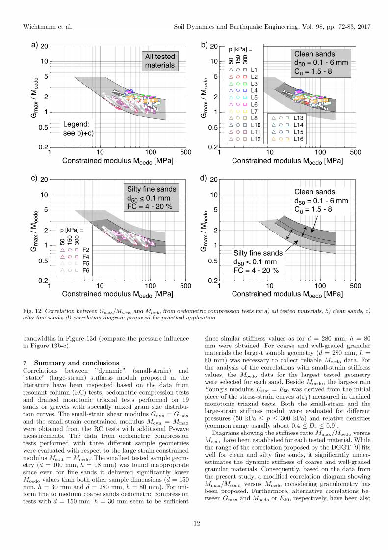
data were already known from the analysis presented inSection 6.1. In Figure 12 the ratio Gmax/Moedo is plottedversus Moedo. Figure 12a presents the data of all testedmaterials, Figure 12b those of all clean sands and gravels(0.1 mm ≤ d50 ≤ 6 mm, 1.5 ≤ Cu ≤ 8, including also datafor L8) and Figure 12c the values for the silty fine sandsF2 - F6. Evidently, for a given material the Gmax/Moedo-Moedo curves in Figure 12 show the same tendencies as theMmax/Moedo-Moedo relationships in Figure 11. Again, thestiffness ratios determined for the clean granular materialslie above those evaluated for the fine sands possessing acertain amount of non-plastic fines. Based on Figure 12b,c,Figure 12d presents a correlation diagram recommendedfor a practical application based on the current experimen-tal study, distinguishing between clean sands and silty finesands.

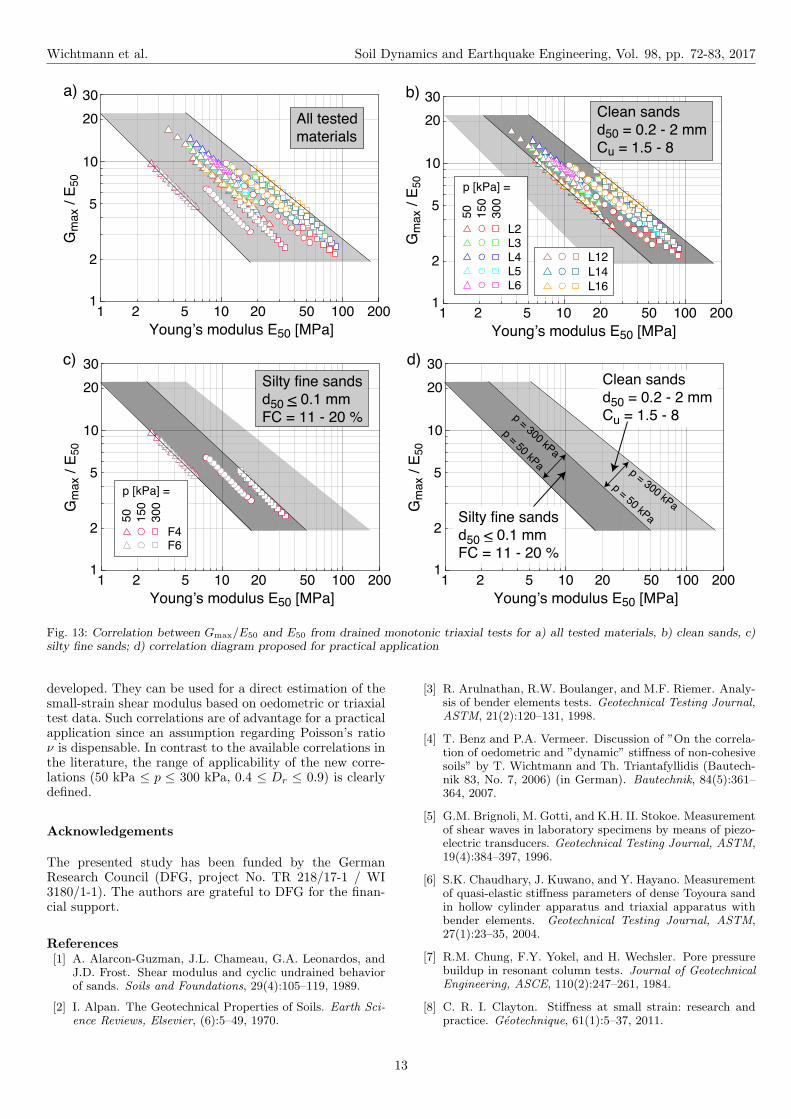
6.3 Correlation between Gmax and E50

A correlation between Gmax and E50 from the drainedmonotonic triaxial tests has been also established, basedon the Young’s moduli calculated from Eq. (6) with theparameters in columns 12 to 14 of Table 2. The correlationhas been evaluated for all ten sands for which E50(e, p)data were available, and for the common ranges of Dr val-ues from the RC and the triaxial tests (Table 3). Figure 13acontains the data for all sands, while the diagrams in Figure13b,c distinguish between the clean sands L2 - L16 (Fig-ure 13b) and the silty sands F2 and F4 (Figure 13c). Forall tested sands and a given pressure, the ratio Gmax/E50

decreases with increasing values of E50. Considering a con-stant value of E50, the ratio Gmax/E50 usually grows withincreasing pressure. For a given pressure, the range of thestiffness ratios obtained for the various clean sands is sim-ilar (Figure 13b), i.e. there is no significant influence ofthe grain size distribution curve. The Gmax/E50 values ofthe silty fine sands lie significantly below those of the cleansands. Therefore, the correlation diagram recommended fora practical application (Figure 13d) distinguishes a rangefor clean granular materials and another one for silty finesands. The correlation shown in Figure 13d can be usedto estimate the dynamic shear modulus directly from theE50 data available from drained monotonic triaxial tests.The pressure-dependence can be considered by choosingthe lower range (for low pressures as p = 50 kPa), themiddle range (for medium pressures as p = 150 kPa) orthe upper range (for high pressures as p = 300 kPa) of the

10


1 10 100 5001

2

5

10

20

50

100

Constrained modulus Moedo [MPa]

Mm

ax / M

oedo

c) clean uniform sands

d50 = 0.35 - 3.5 mm

Cu = 1.5 - 2.0

1 10 100 5001

2

5

10

20

50

100


Mm

ax / M

oedo

d)more well-graded sands

d50 = 0.6 mm

Cu = 2.5 - 8.0

1 10 100 5001

2

5

10

20

50

100


Mm

ax / M

oedo

a)

All tested

materials

Legend:

see b)-d)

DGGT

Benz & Vermeer

(2007)

1 10 100 5001

2

5

10

20

50

100


Mm

ax / M

oedo

b)Clean and silty

fine sands

d50 < 0.2 mm

FC = 0 - 20 %

1 10 100 5001

2

5

10

20

50

100


Mm

ax / M

oedo

e)

Clean and silty

fine sands

d50 < 0.2 mm

FC = 0 - 20 %

Clean uniform sands

d50 = 0.35 - 3.5 mm

Cu = 2.5 - 8.0

L1

F2F4F5F6

50

150

300

p [kPa] =

L2

L11L12

50

150

300

p [kPa] =

L13L14L15L16

L3L4L5L6L7L10

50

150

300

p [kPa] =

Fig. 11: Correlation between Mmax/Moedo and Moedo from oedometric compression tests for a) all tested materials b) clean and siltyfine sands, c) clean uniform medium coarse sands to fine gravels, d) more well-graded clean sands; e) correlation diagram proposedfor practical application

11


F2F4F5F6

50

150

300

p [kPa] =

1 10 100 500


1

0.2

0.5

2

5

10

20

Gm

ax / M

oedo

c)

Silty fine sands

d50 < 0.1 mm

FC = 4 - 20 %

1 10 100 500


1

0.2

0.5

2

5

10

20

Gm

ax / M

oedo

d)

1 10 100 500


1

0.2

0.5

2

5

10

20

Gm

ax / M

oedo

a)

All tested

materials

Legend:

see b)+c)

1 10 100 500


1

0.2

0.5

2

5

10

20

Gm

ax / M

oe

do

b)

L1L2L3L4L5L6L7L8L10L11L12

50

150

300

p [kPa] =

L13L14L15L16

Clean sands

d50 = 0.1 - 6 mm

Cu = 1.5 - 8

Clean sands

d50 = 0.1 - 6 mm

Cu = 1.5 - 8

Silty fine sands

d50 < 0.1 mm

FC = 4 - 20 %

Fig. 12: Correlation between Gmax/Moedo and Moedo from oedometric compression tests for a) all tested materials, b) clean sands, c)silty fine sands; d) correlation diagram proposed for practical application

bandwidths in Figure 13d (compare the pressure influencein Figure 13b-c).

7 Summary and conclusionsCorrelations between ”dynamic” (small-strain) and”static” (large-strain) stiffness moduli proposed in theliterature have been inspected based on the data fromresonant column (RC) tests, oedometric compression testsand drained monotonic triaxial tests performed on 19sands or gravels with specially mixed grain size distribu-tion curves. The small-strain shear modulus Gdyn = Gmax

and the small-strain constrained modulus Mdyn = Mmax

were obtained from the RC tests with additional P-wavemeasurements. The data from oedometric compressiontests performed with three different sample geometrieswere evaluated with respect to the large strain constrainedmodulus Mstat = Moedo. The smallest tested sample geom-etry (d = 100 mm, h = 18 mm) was found inappropriatesince even for fine sands it delivered significantly lowerMoedo values than both other sample dimensions (d = 150mm, h = 30 mm and d = 280 mm, h = 80 mm). For uni-form fine to medium coarse sands oedometric compressiontests with d = 150 mm, h = 30 mm seem to be sufficient

since similar stiffness values as for d = 280 mm, h = 80mm were obtained. For coarse and well-graded granularmaterials the largest sample geometry (d = 280 mm, h =80 mm) was necessary to collect reliable Moedo data. Forthe analysis of the correlations with small-strain stiffnessvalues, the Moedo data for the largest tested geometrywere selected for each sand. Beside Moedo, the large-strainYoung’s modulus Estat = E50 was derived from the initialpiece of the stress-strain curves q(ε1) measured in drainedmonotonic triaxial tests. Both the small-strain and thelarge-strain stiffness moduli were evaluated for differentpressures (50 kPa ≤ p ≤ 300 kPa) and relative densities(common range usually about 0.4 ≤ Dr ≤ 0.9).

Diagrams showing the stiffness ratio Mmax/Moedo versusMoedo have been established for each tested material. Whilethe range of the correlation proposed by the DGGT [9] fitswell for clean and silty fine sands, it significantly under-estimates the dynamic stiffness of coarse and well-gradedgranular materials. Consequently, based on the data fromthe present study, a modified correlation diagram showingMmax/Moedo versus Moedo considering granulometry hasbeen proposed. Furthermore, alternative correlations be-tween Gmax and Moedo or E50, respectively, have been also

12


1 2 5 10 20 50 100 200

Young’s modulus E50 [MPa]

1

2

5

10

20

30

Gm

ax / E

50

a)

1 2 5 10 20 50 100 200


1

2

5

10

20

30

Gm

ax / E

50

b)

L2L3L4L5L6

50

150

300

p [kPa] =

L12

L14

L16

Clean sands

d50 = 0.2 - 2 mm

Cu = 1.5 - 8

F4F6

50

15

0

30

0

p [kPa] =

Silty fine sands

d50 < 0.1 mm

FC = 11 - 20 %

1 2 5 10 20 50 100 200


1

2

5

10

20

30

Gm

ax / E

50

c)

1 2 5 10 20 50 100 200


1

2

5

10

20

30

Gm

ax / E

50

d)

Clean sands

d50 = 0.2 - 2 mm

Cu = 1.5 - 8

Silty fine sands

d50 < 0.1 mm

FC = 11 - 20 %

All tested

materials

p = 300 kPa

p = 300 kPa

p = 50 kPa

p = 50 kPa

Fig. 13: Correlation between Gmax/E50 and E50 from drained monotonic triaxial tests for a) all tested materials, b) clean sands, c)silty fine sands; d) correlation diagram proposed for practical application

developed. They can be used for a direct estimation of thesmall-strain shear modulus based on oedometric or triaxialtest data. Such correlations are of advantage for a practicalapplication since an assumption regarding Poisson’s ratioν is dispensable. In contrast to the available correlations inthe literature, the range of applicability of the new corre-lations (50 kPa ≤ p ≤ 300 kPa, 0.4 ≤ Dr ≤ 0.9) is clearlydefined.

Acknowledgements

The presented study has been funded by the GermanResearch Council (DFG, project No. TR 218/17-1 / WI3180/1-1). The authors are grateful to DFG for the finan-cial support.

References[1] A. Alarcon-Guzman, J.L. Chameau, G.A. Leonardos, and

J.D. Frost. Shear modulus and cyclic undrained behaviorof sands. Soils and Foundations, 29(4):105–119, 1989.

[2] I. Alpan. The Geotechnical Properties of Soils. Earth Sci-ence Reviews, Elsevier, (6):5–49, 1970.

[3] R. Arulnathan, R.W. Boulanger, and M.F. Riemer. Analy-sis of bender elements tests. Geotechnical Testing Journal,ASTM, 21(2):120–131, 1998.

[4] T. Benz and P.A. Vermeer. Discussion of ”On the correla-tion of oedometric and ”dynamic” stiffness of non-cohesivesoils” by T. Wichtmann and Th. Triantafyllidis (Bautech-nik 83, No. 7, 2006) (in German). Bautechnik, 84(5):361–364, 2007.

[5] G.M. Brignoli, M. Gotti, and K.H. II. Stokoe. Measurementof shear waves in laboratory specimens by means of piezo-electric transducers. Geotechnical Testing Journal, ASTM,19(4):384–397, 1996.

[6] S.K. Chaudhary, J. Kuwano, and Y. Hayano. Measurementof quasi-elastic stiffness parameters of dense Toyoura sandin hollow cylinder apparatus and triaxial apparatus withbender elements. Geotechnical Testing Journal, ASTM,27(1):23–35, 2004.

[7] R.M. Chung, F.Y. Yokel, and H. Wechsler. Pore pressurebuildup in resonant column tests. Journal of GeotechnicalEngineering, ASCE, 110(2):247–261, 1984.

[8] C. R. I. Clayton. Stiffness at small strain: research andpractice. Geotechnique, 61(1):5–37, 2011.

13


[9] DGGT. Empfehlungen des Arbeitskreises 1.4 ”Baugrund-dynamik” der Deutschen Gesellschaft fur Geotechnik e.V.,2002.

[10] C.S. El Mohtar, V.P. Drnevich, M. Santagata, and A. Bo-bet. Combined resonant column and cyclic triaxial testsfor measuring undrained shear modulus reduction of sandwith plastic fines. Geotechnical Testing Journal, ASTM,36(4):1–9, 2013.

[11] V. Fioravante. Anisotropy of small strain stiffness of Ticinoand Kenya sands from seismic wave propagation measuredin triaxial testing. Soils and Foundations, 40(4):129–142,2000.

[12] V. Fioravante and R. Capoferri. On the use of multi-directional piezoelectric transducers in triaxial testing.Geotechnical Testing Journal, ASTM, 24(3):243–255, 2001.

[13] B.O. Hardin and W.L. Black. Sand stiffness under var-ious triaxial stresses. Journal of the Soil Mechanics andFoundations Division, ASCE, 92(SM2):27–42, 1966.

[14] B.O. Hardin and V.P. Drnevich. Shear modulus and damp-ing in soils: measurement and parameter effects. Journalof the Soil Mechanics and Foundations Division, ASCE,98(SM6):603–624, 1972.

[15] B.O. Hardin and M.E. Kalinski. Estimating the shear mod-ulus of gravelly soils. Journal of Geotechnical and Geoen-vironmental Engineering, ASCE, 131(7):867–875, 2005.

[16] B.O. Hardin and F.E. Richart Jr. Elastic wave velocitiesin granular soils. Journal of the Soil Mechanics and Foun-dations Division, ASCE, 89(SM1):33–65, 1963.

[17] H. Hertz. Uber die Beruhrung fester elastischer Korper.Journal reine und angewandte Mathematik, 92:156–171,1881.

[18] K. Ishihara. Liquefaction and flow failure during earth-quakes. The 33rd Rankine Lecture. Geotechnique,43(3):351–415, 1993.

[19] K. Ishihara. Soil Behaviour in Earthquake Geotechnics.Oxford Science Publications, 1996.

[20] T. Iwasaki, F. Tatsuoka, and Y. Takagi. Shear moduli ofsands under cyclic torsional shear loading. Soils and Foun-dations, 18(1):39–56, 1978.

[21] F. Jafarzadeh and H. Sadeghi. Experimental study on dy-namic properties of sand with emphasis on the degree ofsaturation. Soil Dynamics and Earthquake Engineering,32:26–41, 2012.

[22] T. Kokusho. Cyclic triaxial test of dynamic soil propertiesfor wide strain range. Soils and Foundations, 20(2):45–59,1980.

[23] S.L. Kramer. Geotechnical earthquake engineering.Prentice-Hall, Upper Saddle River, N.J., 1996.

[24] G. Lanzo, M. Vucetic, and M. Doroudian. Reduction ofshear modulus at small strains in simple shear. Journalof Geotechnical and Geoenvironmental Engineering, ASCE,123(11):1035–1042, 1997.

[25] X.S. Li and Z.Y. Cai. Effects of low-number previbra-tion cycles on dynamic properties of dry sand. Journalof Geotechnical and Geoenvironmental Engineering, ASCE,125(11):979–987, 1999.

[26] X.S. Li, W.L. Yang, C.K. Chen, and W.C. Wang. Energy-injecting virtual mass resonant column system. Journalof Geotechnical and Geoenvironmental Engineering, ASCE,124(5):428–438, 1998.

[27] D.C.F. Lo Presti, M. Jamiolkowski, O. Pallara, A. Caval-laro, and Pedroni S. Shear modulus and damping of soils.Geotechnique, 47(3):603–617, 1997.

[28] D.C.F. Lo Presti, O. Pallara, R. Lancellotta, M. Armandi,and R. Maniscalco. Monotonic and cyclic loading behaviourof two sands at small strains. Geotechnical Testing Journal,ASTM, (4):409–424, 1993.

[29] F.-Y. Menq and K.H. Stokoe II. Linear dynamic propertiesof sandy and gravelly soils from large-scale resonant tests.In Di Benedetto et al., editor, Deformation Characteristicsof Geomaterials, pages 63–71. Swets & Zeitlinger, Lisse,2003.

[30] R.D. Mindlin and H. Deresiewicz. Elastic spheres in contactunder varying oblique forces. Journal of Applied Mechanics,20:327–344, 1953.

[31] F. Radjai and D.E. Wolf. Features of static pressure indense granular media. Granular Matter, (1):3–8, 1998.

[32] F. Radjai, D.E. Wolf, M. Jean, and J.-J. Moreau. Bimodalcharacter of stress transmission in granular packings. Phys-ical Review Lett., 80(1):61–64, 1998.

[33] R.P. Ray and R.D. Woods. Modulus and damping due touniform and variable cyclic loading. Journal of Geotechni-cal Engineering, ASCE, 114(8):861–876, 1988.

[34] S.K. Saxena and K.R. Reddy. Dynamic moduli and damp-ing ratios for Monterey No. 0 sand by resonant columntests. Soils and Foundations, 29(2):37–51, 1989.

[35] C.K. Shen, X.S. Li, and Y.Z. Gu. Microcomputer basedfree torsional vibration test. Journal of Geotechnical Engi-neering, ASCE, 111(8):971–986, 1985.

[36] I. Towhata. Geotechnical Earthquake Engineering.Springer, 2008.

[37] M. Vucetic. Cyclic threshold shear strains in soils. Journalof Geotechnical Engineering, ASCE, 120(12):2208–2228,1994.

[38] Y.-H. Wang and K.-Y. Tsui. Experimental characteriza-tion of dynamic property changes in aged sands. Journalof Geotechnical and Geoenvironmental Engineering, ASCE,135(2):259–270, 2009.

[39] T. Wichtmann, M.A. Navarrete Hernandez, and T. Tri-antafyllidis. On the influence of a non-cohesive content offines on the small strain stiffness of quartz sand. Soil Dy-namics and Earthquake Engineering, 69(2):103–114, 2014.

[40] T. Wichtmann, A. Niemunis, and T. Triantafyllidis. Im-proved simplified calibration procedure for a high-cycle ac-cumulation model. Soil Dynamics and Earthquake Engi-neering, 70(3):118–132, 2015.

[41] T. Wichtmann and T. Triantafyllidis. Influence of the grainsize distribution curve of quartz sand on the small strainshear modulus Gmax. Journal of Geotechnical and Geoen-vironmental Engineering, ASCE, 135(10):1404–1418, 2009.

[42] T. Wichtmann and T. Triantafyllidis. On the influenceof the grain size distribution curve on P-wave velocity,constrained elastic modulus Mmax and Poisson’s ratio ofquartz sands. Soil Dynamics and Earthquake Engineering,30(8):757–766, 2010.

[43] T. Wichtmann and T. Triantafyllidis. Effect of uniformitycoefficient on G/Gmax and damping ratio of uniform to wellgraded quartz sands. Journal of Geotechnical and Geoen-vironmental Engineering, ASCE, 139(1):59–72, 2013.

[44] T. Wichtmann and Th. Triantafyllidis. Uber die Korrela-tion der odometrischen und der ”dynamischen” Steifigkeitnichtbindiger Boden. Bautechnik, 83(7):482 – 491, 2006.

[45] T. Wichtmann and Th. Triantafyllidis. Reply to the discus-sion of T. Benz and P.A. Vermeer on ”On the correlationof oedometric and ”dynamic” stiffness of non-cohesive soils(Bautechnik 83, No. 7, 2006) (in German). Bautechnik,84(5):364–366, 2007.

14


[46] T. Wichtmann and Th. Triantafyllidis. On the correlationof ”static” and ”dynamic” stiffness moduli of non-cohesivesoils. Bautechnik, Special Issue ”Geotechnical Engineer-ing”, July 2009, pages 28–39, 2009.

[47] J. Yang and X.Q. Gu. Shear stiffness of granular material atsmall strains: Does it depend on grain size? Geotechnique,63(2):165–179, 2013.

[48] P. Yu. Discussion of ”Moduli and Damping Factors forDynamic Analyses of Cohesionless Soils” by Seed et al.Journal of Geotechnical Engineering, ASCE, 114(8):954–957, 1988.

[49] J. Zhang, R.D. Andrus, and C.H. Juang. Normalized shearmodulus and material damping ratio relationships. Journalof Geotechnical and Geoenvironmental Engineering, ASCE,131(4):453–464, 2005.

15

on correlations between ”dynamic” (small-strain) and ... · on correlations between...

Documents