on admissible eigenvalue approximations from krylov ... · on admissible eigenvalue approximations...
TRANSCRIPT
On admissible eigenvalue approximations from
Krylov subspace methods for non-normal matrices
Jurjen Duintjer Tebbens
joint work with
Gérard Meurant
Crouzeix’s conjecture workshopAIM, San Jose, US, August 3, 2017.
1
Outline
Outline
1 Introduction
2 Ritz values
3 Harmonic Ritz values, GMRES and FOM polynomials
2

Outline
1 Introduction
3

Introduction
This talk is about some iterative methods designed for large, sparse matrices tofind eigenvalues, eigenvectors and solutions of linear systems.
4
Introduction
This talk is about some iterative methods designed for large, sparse matrices tofind eigenvalues, eigenvectors and solutions of linear systems.
More precisely, it is about Krylov subspace methods generating during the kthiteration the kth Krylov subspace
Kk(A, v) ≡ span{v, Av, . . . , Ak−1v}for a given a nonsingular matrix and nonzero vector
A ∈ Cn×n, v ∈ Cn (w.l.o.g. ‖v‖ = 1).
Note that
all vectors w ∈ Kk(A, v) = span{v, Av, ..., Ak−1v} are of the form
w = α0v + α1Av + · · · + αk−1Ak−1v = pk−1(A)v
for a polynomial pk−1 of degree k − 1.
we always consider both the matrix A and a starting vector v and theirinterplay can be crucial (also if we are in properties like the field of valuesor matrix polynomials which depend on the matrix only).
We will restrict ourselves to non-normal matrices (for which Crouzeix’sconjecture has not yet been proved).
4

Introduction
With non-normal matrices, we can very roughly divide the available methodsinto those using short recurrences (lower compuational costs) and those usinglong recurrences (enhanced stability properties).
5

Introduction
With non-normal matrices, we can very roughly divide the available methodsinto those using short recurrences (lower compuational costs) and those usinglong recurrences (enhanced stability properties).
We focus on the last class which is based on the Arnoldi orthogonalizationprocess [Arnoldi - 1951] for computing orthogonal bases of the Krylov subspaces.
5
Introduction
With non-normal matrices, we can very roughly divide the available methodsinto those using short recurrences (lower compuational costs) and those usinglong recurrences (enhanced stability properties).
We focus on the last class which is based on the Arnoldi orthogonalizationprocess [Arnoldi - 1951] for computing orthogonal bases of the Krylov subspaces.
In the kth iteration of the process (without breakdown) it computes thedecomposition
AVk = Vk+1Hk,
where the columns of Vk = [v1, . . . , vk] (the Arnoldi vectors) contain anorthogonal basis for the kth Krylov subspace Kk(A, v) and Hk is rectangularupper Hessenberg.
By deleting the last row we get the square matrix
Hk = V ∗
k AVk ∈ Ck×k;
Hk is the orthogonal restriction of A onto Kk(A, v) and A is a dilation of Hk.
5
Introduction
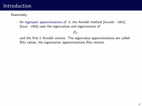
Essentially,
- for eigenpair approximations of A, the Arnoldi method [Arnoldi - 1951],
[Saad - 1980] uses the eigenvalues and eigenvectors of
Hk
and the first k Arnoldi vectors. The eigenvalue approximations are calledRitz values, the eigenvector approximations Ritz vectors.
6
Introduction
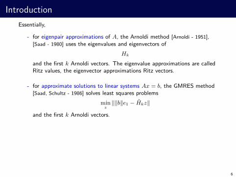
Essentially,
- for eigenpair approximations of A, the Arnoldi method [Arnoldi - 1951],
[Saad - 1980] uses the eigenvalues and eigenvectors of
Hk
and the first k Arnoldi vectors. The eigenvalue approximations are calledRitz values, the eigenvector approximations Ritz vectors.
- for approximate solutions to linear systems Ax = b, the GMRES method[Saad, Schultz - 1986] solves least squares problems
minz
‖‖b‖e1 − Hkz‖
and the first k Arnoldi vectors.
6
Introduction
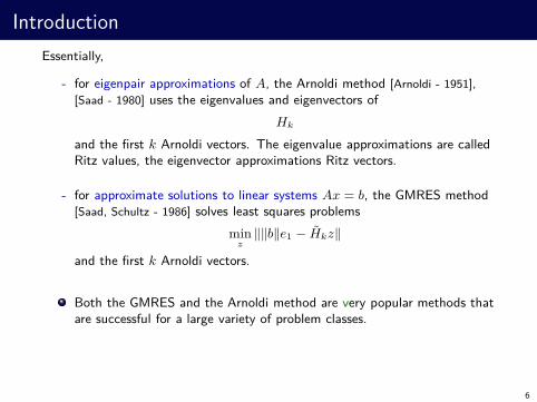
Essentially,
- for eigenpair approximations of A, the Arnoldi method [Arnoldi - 1951],
[Saad - 1980] uses the eigenvalues and eigenvectors of
Hk
and the first k Arnoldi vectors. The eigenvalue approximations are calledRitz values, the eigenvector approximations Ritz vectors.
- for approximate solutions to linear systems Ax = b, the GMRES method[Saad, Schultz - 1986] solves least squares problems
minz
‖‖b‖e1 − Hkz‖
and the first k Arnoldi vectors.
Both the GMRES and the Arnoldi method are very popular methods thatare successful for a large variety of problem classes.
6
Introduction
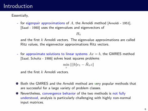
Essentially,
- for eigenpair approximations of A, the Arnoldi method [Arnoldi - 1951],
[Saad - 1980] uses the eigenvalues and eigenvectors of
Hk
and the first k Arnoldi vectors. The eigenvalue approximations are calledRitz values, the eigenvector approximations Ritz vectors.
- for approximate solutions to linear systems Ax = b, the GMRES method[Saad, Schultz - 1986] solves least squares problems
minz
‖‖b‖e1 − Hkz‖
and the first k Arnoldi vectors.
Both the GMRES and the Arnoldi method are very popular methods thatare successful for a large variety of problem classes.
Nevertheless, convergence behavior of the two methods is not fullyunderstood, analysis is particularly challenging with highly non-normalinput matrices.
6

Introduction
Often one tries to use the tools that are successful for analysis ofhermitian counterparts of GMRES and Arnoldi like the ConjugateGradients and the Lanczos method.
7
Introduction
Often one tries to use the tools that are successful for analysis ofhermitian counterparts of GMRES and Arnoldi like the ConjugateGradients and the Lanczos method.
For example, the basic tool for explaining Krylov subspace methods forhermitian linear systems is the eigenvalue distribution.
However, for GMRES it is known for some time that if GMRES generatesa certain residual norm history, the same history can be generated withany nonzero spectrum [Greenbaum, Strakoš - 1994].
Complemented with the fact that GMRES can generate arbitrarynon-increasing residual norms, this gives the result that anynon-increasing convergence curve is possible with any nonzero spectrum[Greenbaum , Pták, Strakoš - 1996].
A complete description of the class of matrices and right hand sides withprescribed convergence and eigenvalues was given in [Arioli , Pták, Strakoš
- 1998].
7
Convergence analysis for Krylov subspace methods
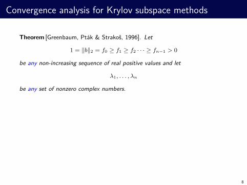
Theorem [Greenbaum, Pták & Strakoš, 1996]. Let
1 = ‖b‖2 = f0 ≥ f1 ≥ f2 · · · ≥ fn−1 > 0
be any non-increasing sequence of real positive values and let
λ1, . . . , λn
be any set of nonzero complex numbers.
8
Convergence analysis for Krylov subspace methods
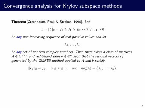
Theorem [Greenbaum, Pták & Strakoš, 1996]. Let
1 = ‖b‖2 = f0 ≥ f1 ≥ f2 · · · ≥ fn−1 > 0
be any non-increasing sequence of real positive values and let
λ1, . . . , λn
be any set of nonzero complex numbers. Then there exists a class of matrices
A ∈ Cn×n and right-hand sides b ∈ Cn such that the residual vectors rk
generated by the GMRES method applied to A and b satisfy
‖rk‖2 = fk, 0 ≤ k ≤ n, and eig(A) = {λ1, . . . , λn}.
8
Convergence analysis for Krylov subspace methods
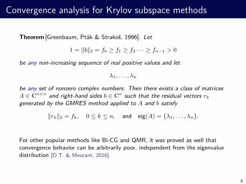
Theorem [Greenbaum, Pták & Strakoš, 1996]. Let
1 = ‖b‖2 = f0 ≥ f1 ≥ f2 · · · ≥ fn−1 > 0
be any non-increasing sequence of real positive values and let
λ1, . . . , λn
be any set of nonzero complex numbers. Then there exists a class of matrices
A ∈ Cn×n and right-hand sides b ∈ Cn such that the residual vectors rk
generated by the GMRES method applied to A and b satisfy
‖rk‖2 = fk, 0 ≤ k ≤ n, and eig(A) = {λ1, . . . , λn}.
For other popular methods like Bi-CG and QMR, it was proved as well thatconvergence behavior can be arbitrarily poor, independent from the eigenvaluedistribution [D.T. & Meurant, 2016].
8
Introduction
Other objects have been successful in explaining GMRES for particularproblems, including:
9
Introduction
Other objects have been successful in explaining GMRES for particularproblems, including:
The pseudo-spectrum, see e.g. [Trefethen, Embree - 2005],
9
Introduction
Other objects have been successful in explaining GMRES for particularproblems, including:
The pseudo-spectrum, see e.g. [Trefethen, Embree - 2005],
the field of values, see e.g. [Eiermann - 1993],
9
Introduction
Other objects have been successful in explaining GMRES for particularproblems, including:
The pseudo-spectrum, see e.g. [Trefethen, Embree - 2005],
the field of values, see e.g. [Eiermann - 1993],
the numerical polynomial hull, see e.g. [Greenbaum - 2002],
9
Introduction
Other objects have been successful in explaining GMRES for particularproblems, including:
The pseudo-spectrum, see e.g. [Trefethen, Embree - 2005],
the field of values, see e.g. [Eiermann - 1993],
the numerical polynomial hull, see e.g. [Greenbaum - 2002],
the Ritz values, i.e. the eigenvalues of the Hessenberg matrices generatedby the underlying Arnoldi process, see e.g. [van der Vorst, Vuik - 1993].
Although in practice eigenvalues do often influence convergence of GMRES,they cannot be used as a universal tool for explaining GMRES and such a toolis unlikely to exist.
9
Introduction
An important tool for hermitian eigenproblems solved with Krylov subspacemethods is the following interlacing property:
10
Introduction
An important tool for hermitian eigenproblems solved with Krylov subspacemethods is the following interlacing property:
Consider a tridiagonal Jacobi matrix Tm and its leading principal submatrix Tk
for some k < m. If the ordered eigenvalues of T k are
ρ(k)1 < ρ
(k)2 < . . . < ρ
(k)k ,
then in every open interval between two subsequent eigenvalues
(ρ(k)i−1, ρ
(k)i ), i = 2, . . . , k,
there lies at least one eigenvalue of Tm.
10

Introduction
An important tool for hermitian eigenproblems solved with Krylov subspacemethods is the following interlacing property:
Consider a tridiagonal Jacobi matrix Tm and its leading principal submatrix Tk
for some k < m. If the ordered eigenvalues of T k are
ρ(k)1 < ρ
(k)2 < . . . < ρ
(k)k ,
then in every open interval between two subsequent eigenvalues
(ρ(k)i−1, ρ
(k)i ), i = 2, . . . , k,
there lies at least one eigenvalue of Tm.
This interlacing property enables, among others, to prove the persistencetheorem (see [Paige - 1971, 1976, 1980] or [Meurant, Strakoš - 2006]) which iscrucial for controlling the convergence of Ritz values in the Lanczos method.
10
Introduction
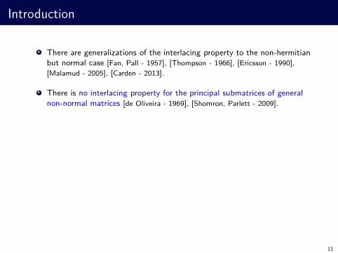
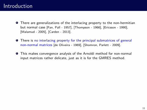
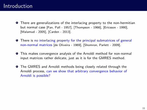
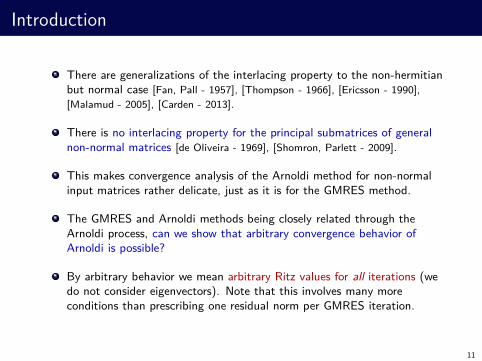
There are generalizations of the interlacing property to the non-hermitianbut normal case [Fan, Pall - 1957], [Thompson - 1966], [Ericsson - 1990],
[Malamud - 2005], [Carden - 2013].
11
Introduction
There are generalizations of the interlacing property to the non-hermitianbut normal case [Fan, Pall - 1957], [Thompson - 1966], [Ericsson - 1990],
[Malamud - 2005], [Carden - 2013].
There is no interlacing property for the principal submatrices of generalnon-normal matrices [de Oliveira - 1969], [Shomron, Parlett - 2009].
This makes convergence analysis of the Arnoldi method for non-normalinput matrices rather delicate, just as it is for the GMRES method.
The GMRES and Arnoldi methods being closely related through theArnoldi process, can we show that arbitrary convergence behavior ofArnoldi is possible?
By arbitrary behavior we mean arbitrary Ritz values for all iterations (wedo not consider eigenvectors). Note that this involves many moreconditions than prescribing one residual norm per GMRES iteration.
11
2. Prescribed convergence for Arnoldi’s method
Notation: Let the kth Hessenberg matrix Hk generated in Arnoldi’s methodhave the eigenvalue ρ and eigenvector y,
Hk y = ρ y.
Then
12
2. Prescribed convergence for Arnoldi’s method
Notation: Let the kth Hessenberg matrix Hk generated in Arnoldi’s methodhave the eigenvalue ρ and eigenvector y,
Hk y = ρ y.
Then
ρ is a Ritz value for A
Vky is a Ritz vector for A
12
2. Prescribed convergence for Arnoldi’s method
Notation: Let the kth Hessenberg matrix Hk generated in Arnoldi’s methodhave the eigenvalue ρ and eigenvector y,
Hk y = ρ y.
Then
ρ is a Ritz value for A
Vky is a Ritz vector for A
With the Arnoldi decomposition AVk = Vk+1Hk, we obtain for the Ritz-valueRitz-vector pair {ρ, Vky} the residual norm:
‖A(Vky)−ρ(Vky)‖ = ‖A(Vky)−VkHky‖ = ‖Vk+1Hky−VkHky‖ = hk+1,k|eTk y|.
Often for small hk+1,k|eTk y|, the Arnoldi method takes {ρ, Vky} as an
approximate eigenvalue-eigenvector pair of A. Note that a small value
hk+1,k|eTk y| needs not imply that ρ is close to a true eigenvalue of A, see e.g.
[Chatelin - 1993], [Godet-Thobie - 1993]; convergence analysis cannot be based on
this value but focusses instead on the quality of approximate invariant
subspaces [Beattie, Embree, Sorensen - 2005].
12
2. Prescribed convergence for Arnoldi’s method
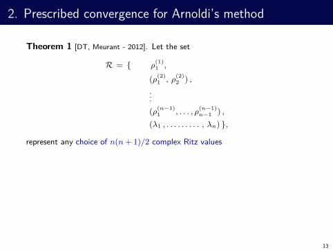
Theorem 1 [DT, Meurant - 2012]. Let the set
R = { ρ(1)1 ,
(ρ(2)1 , ρ
(2)2 ) ,
...
(ρ(n−1)1 , . . . , ρ
(n−1)n−1 ) ,
(λ1 , . . . . . . . . . , λn) },
represent any choice of n(n + 1)/2 complex Ritz values
13
2. Prescribed convergence for Arnoldi’s method
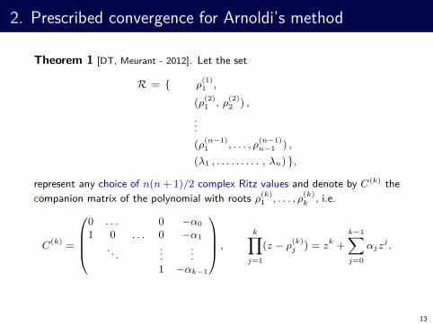
Theorem 1 [DT, Meurant - 2012]. Let the set
R = { ρ(1)1 ,
(ρ(2)1 , ρ
(2)2 ) ,
...
(ρ(n−1)1 , . . . , ρ
(n−1)n−1 ) ,
(λ1 , . . . . . . . . . , λn) },
represent any choice of n(n + 1)/2 complex Ritz values and denote by C(k) the
companion matrix of the polynomial with roots ρ(k)1 , . . . , ρ
(k)k , i.e.
C(k) =
0 . . . 0 −α0
1 0 . . . 0 −α1
. . ....
...1 −αk−1
,
k∏
j=1
(z − ρ(k)j ) = zk +
k−1∑
j=0
αjzj .
13
2. Prescribed convergence for Arnoldi’s method
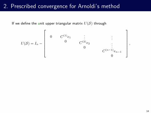
If we define the unit upper triangular matrix U(S) through
U(S) = In −
0 C(1)e1
0
...
C(2)e2
0
...
...
C(n−1)en−1
0
,
14
2. Prescribed convergence for Arnoldi’s method
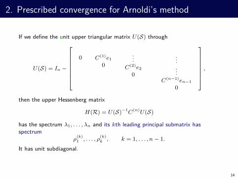
If we define the unit upper triangular matrix U(S) through
U(S) = In −
0 C(1)e1
0
...
C(2)e2
0
...
...
C(n−1)en−1
0
,
then the upper Hessenberg matrix
H(R) = U(S)−1C(n)U(S)
has the spectrum λ1, . . . , λn and its kth leading principal submatrix hasspectrum
ρ(k)1 , . . . , ρ
(k)k , k = 1, . . . , n − 1.
It has unit subdiagonal.
14

2. Prescribed convergence for Arnoldi’s method
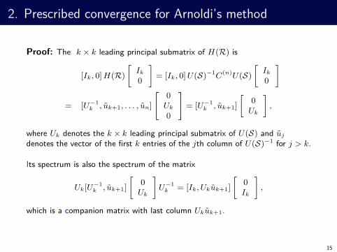
Proof: The k × k leading principal submatrix of H(R) is
[Ik, 0] H(R)
[
Ik
0
]
= [Ik, 0] U(S)−1C(n)U(S)
[
Ik
0
]
= [U−1k , uk+1, . . . , un]
[
0Uk
0
]
= [U−1k , uk+1]
[
0Uk
]
,
where Uk denotes the k × k leading principal submatrix of U(S) and uj
denotes the vector of the first k entries of the jth column of U(S)−1 for j > k.
15
2. Prescribed convergence for Arnoldi’s method
Proof: The k × k leading principal submatrix of H(R) is
[Ik, 0] H(R)
[
Ik
0
]
= [Ik, 0] U(S)−1C(n)U(S)
[
Ik
0
]
= [U−1k , uk+1, . . . , un]
[
0Uk
0
]
= [U−1k , uk+1]
[
0Uk
]
,
where Uk denotes the k × k leading principal submatrix of U(S) and uj
denotes the vector of the first k entries of the jth column of U(S)−1 for j > k.
Its spectrum is also the spectrum of the matrix
Uk[U−1k , uk+1]
[
0Uk
]
U−1k = [Ik, Ukuk+1]
[
0Ik
]
,
which is a companion matrix with last column Ukuk+1.
15
2. Prescribed convergence for Arnoldi’s method
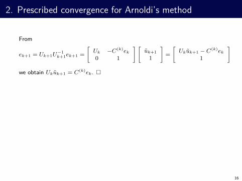
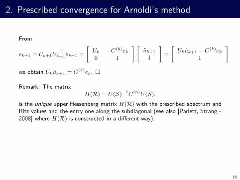
From
ek+1 = Uk+1U−1k+1ek+1 =
[
Uk −C(k)ek
0 1
] [
uk+1
1
]
=
[
Ukuk+1 − C(k)ek
1
]
we obtain Ukuk+1 = C(k)ek. �
16
2. Prescribed convergence for Arnoldi’s method
From
ek+1 = Uk+1U−1k+1ek+1 =
[
Uk −C(k)ek
0 1
] [
uk+1
1
]
=
[
Ukuk+1 − C(k)ek
1
]
we obtain Ukuk+1 = C(k)ek. �
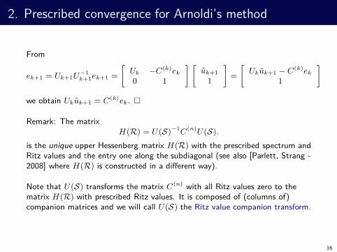
Remark: The matrixH(R) = U(S)−1C(n)U(S).
is the unique upper Hessenberg matrix H(R) with the prescribed spectrum andRitz values and the entry one along the subdiagonal (see also [Parlett, Strang -2008] where H(R) is constructed in a different way).
16
2. Prescribed convergence for Arnoldi’s method
From
ek+1 = Uk+1U−1k+1ek+1 =
[
Uk −C(k)ek
0 1
] [
uk+1
1
]
=
[
Ukuk+1 − C(k)ek
1
]
we obtain Ukuk+1 = C(k)ek. �
Remark: The matrixH(R) = U(S)−1C(n)U(S).
is the unique upper Hessenberg matrix H(R) with the prescribed spectrum andRitz values and the entry one along the subdiagonal (see also [Parlett, Strang -2008] where H(R) is constructed in a different way).
Note that U(S) transforms the matrix C(n) with all Ritz values zero to thematrix H(R) with prescribed Ritz values. It is composed of (columns of)companion matrices and we will call U(S) the Ritz value companion transform.
16
2. Prescribed convergence for Arnoldi’s method
Thus the Ritz values generated in the Arnoldi method can exhibit anyconvergence behavior: It suffices to apply the Arnoldi process with the initialArnoldi vector e1 and the matrix H(R) with arbitrarily prescribed Ritz values.Then the method generates the Hessenberg matrix H(R) itself.
17
2. Prescribed convergence for Arnoldi’s method
Thus the Ritz values generated in the Arnoldi method can exhibit anyconvergence behavior: It suffices to apply the Arnoldi process with the initialArnoldi vector e1 and the matrix H(R) with arbitrarily prescribed Ritz values.Then the method generates the Hessenberg matrix H(R) itself.
Question: Can the same prescribed Ritz values be generated with positiveentries other than one on the subdiagonal?
For σ1, σ2, . . . , σn−1 > 0 consider the diagonal similarity transformation
H ≡ diag (1, σ1, σ1σ2, . . . , Πn−1j=1 σj) H(R)
(
diag (1, σ1, σ1σ2, . . . , Πn−1j=1 σj)
)
−1.
Then the subdiagonal of H has the entries σ1, σ2, . . . , σn−1 and all leadingprincipal submatrices of H are similar the corresponding leading principalsubmatrices of H(R).
17
2. Prescribed convergence for Arnoldi’s method
This immediately leads to a parametrization of the matrices and initial Arnoldivectors that generate a given set of Ritz values R:
18
2. Prescribed convergence for Arnoldi’s method
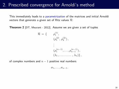
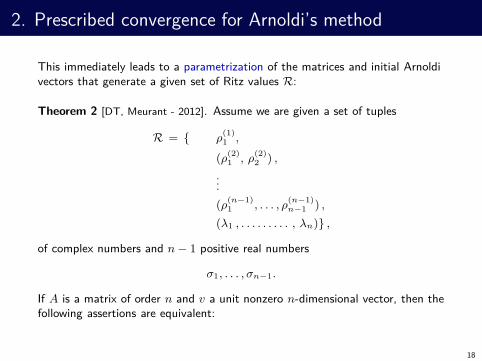
This immediately leads to a parametrization of the matrices and initial Arnoldivectors that generate a given set of Ritz values R:
Theorem 2 [DT, Meurant - 2012]. Assume we are given a set of tuples
R = { ρ(1)1 ,
(ρ(2)1 , ρ
(2)2 ) ,
...
(ρ(n−1)1 , . . . , ρ
(n−1)n−1 ) ,
(λ1 , . . . . . . . . . , λn)} ,
of complex numbers and n − 1 positive real numbers
σ1, . . . , σn−1.
18
2. Prescribed convergence for Arnoldi’s method
This immediately leads to a parametrization of the matrices and initial Arnoldivectors that generate a given set of Ritz values R:
Theorem 2 [DT, Meurant - 2012]. Assume we are given a set of tuples
R = { ρ(1)1 ,
(ρ(2)1 , ρ
(2)2 ) ,
...
(ρ(n−1)1 , . . . , ρ
(n−1)n−1 ) ,
(λ1 , . . . . . . . . . , λn)} ,
of complex numbers and n − 1 positive real numbers
σ1, . . . , σn−1.
If A is a matrix of order n and v a unit nonzero n-dimensional vector, then thefollowing assertions are equivalent:
18
2. Prescribed convergence for Arnoldi’s method
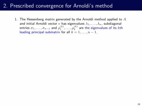
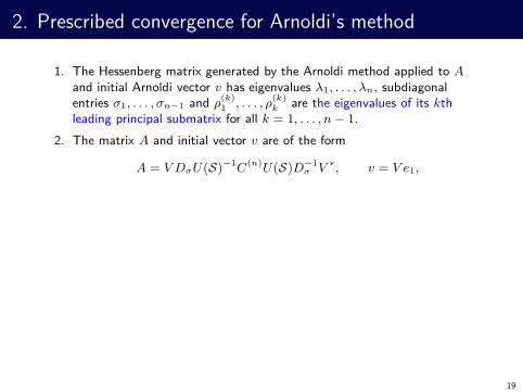
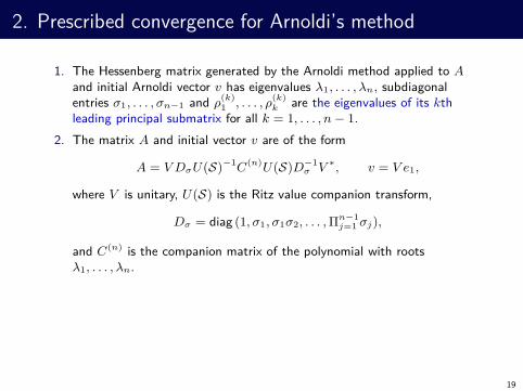
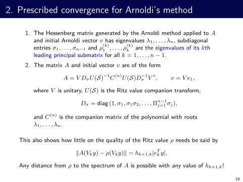
1. The Hessenberg matrix generated by the Arnoldi method applied to Aand initial Arnoldi vector v has eigenvalues λ1, . . . , λn, subdiagonalentries σ1, . . . , σn−1 and ρ
(k)1 , . . . , ρ
(k)k are the eigenvalues of its kth
leading principal submatrix for all k = 1, . . . , n − 1.
19
2. Prescribed convergence for Arnoldi’s method
1. The Hessenberg matrix generated by the Arnoldi method applied to Aand initial Arnoldi vector v has eigenvalues λ1, . . . , λn, subdiagonalentries σ1, . . . , σn−1 and ρ
(k)1 , . . . , ρ
(k)k are the eigenvalues of its kth
leading principal submatrix for all k = 1, . . . , n − 1.
2. The matrix A and initial vector v are of the form
A = V DσU(S)−1C(n)U(S)D−1σ V ∗, v = V e1,
where V is unitary, U(S) is the Ritz value companion transform,
Dσ = diag (1, σ1, σ1σ2, . . . , Πn−1j=1 σj),
and C(n) is the companion matrix of the polynomial with rootsλ1, . . . , λn.
This also shows how little on the quality of the Ritz value ρ needs be said by
‖A(Vky) − ρ(Vky)‖ = hk+1,k|eTk y|.
Any distance from ρ to the spectrum of A is possible with any value of hk+1,k!
19
2. Prescribed convergence for Arnoldi’s method
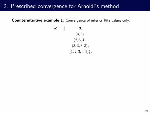
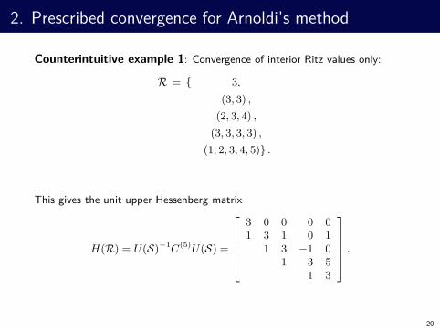
Counterintuitive example 1: Convergence of interior Ritz values only:
R = { 3,
(3, 3) ,
(2, 3, 4) ,
(3, 3, 3, 3) ,
(1, 2, 3, 4, 5)} .
20
2. Prescribed convergence for Arnoldi’s method
Counterintuitive example 1: Convergence of interior Ritz values only:
R = { 3,
(3, 3) ,
(2, 3, 4) ,
(3, 3, 3, 3) ,
(1, 2, 3, 4, 5)} .
This gives the unit upper Hessenberg matrix
H(R) = U(S)−1C(5)U(S) =
3 0 0 0 01 3 1 0 1
1 3 −1 01 3 5
1 3
.
20
2. Prescribed convergence for Arnoldi’s method
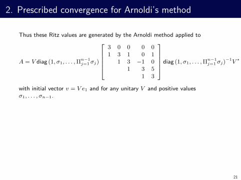
Thus these Ritz values are generated by the Arnoldi method applied to
A = V diag (1, σ1, . . . , Πn−1j=1 σj)
3 0 0 0 01 3 1 0 1
1 3 −1 01 3 5
1 3
diag (1, σ1, . . . , Πn−1j=1 σj)−1V ∗
with initial vector v = V e1 and for any unitary V and positive valuesσ1, . . . , σn−1.
21
2. Prescribed convergence for Arnoldi’s method
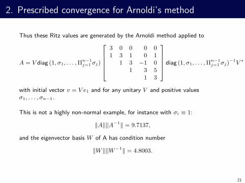
Thus these Ritz values are generated by the Arnoldi method applied to
A = V diag (1, σ1, . . . , Πn−1j=1 σj)
3 0 0 0 01 3 1 0 1
1 3 −1 01 3 5
1 3
diag (1, σ1, . . . , Πn−1j=1 σj)−1V ∗
with initial vector v = V e1 and for any unitary V and positive valuesσ1, . . . , σn−1.
This is not a highly non-normal example, for instance with σi ≡ 1:
‖A‖‖A−1‖ = 9.7137,
and the eigenvector basis W of A has condition number
‖W ‖‖W −1‖ = 4.8003.
21
2. Prescribed convergence for Arnoldi’s method
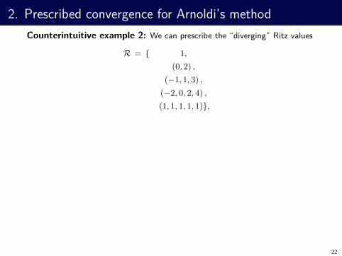
Counterintuitive example 2: We can prescribe the “diverging” Ritz values
R = { 1,
(0, 2) ,
(−1, 1, 3) ,
(−2, 0, 2, 4) ,
(1, 1, 1, 1, 1)},
22
2. Prescribed convergence for Arnoldi’s method
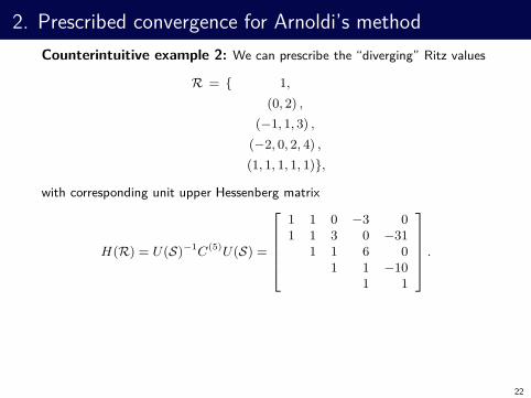
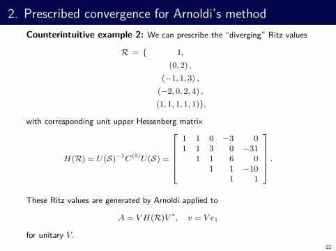
Counterintuitive example 2: We can prescribe the “diverging” Ritz values
R = { 1,
(0, 2) ,
(−1, 1, 3) ,
(−2, 0, 2, 4) ,
(1, 1, 1, 1, 1)},
with corresponding unit upper Hessenberg matrix
H(R) = U(S)−1C(5)U(S) =
1 1 0 −3 01 1 3 0 −31
1 1 6 01 1 −10
1 1
.
22
2. Prescribed convergence for Arnoldi’s method
Counterintuitive example 2: We can prescribe the “diverging” Ritz values
R = { 1,
(0, 2) ,
(−1, 1, 3) ,
(−2, 0, 2, 4) ,
(1, 1, 1, 1, 1)},
with corresponding unit upper Hessenberg matrix
H(R) = U(S)−1C(5)U(S) =
1 1 0 −3 01 1 3 0 −31
1 1 6 01 1 −10
1 1
.
These Ritz values are generated by Arnoldi applied to
A = V H(R)V ∗, v = V e1
for unitary V.
22
2. Prescribed convergence for Arnoldi’s method
The same “diverging” Ritz values are generated with the exponentiallydecreasing values 2−1, 2−2, 2−3 and 2−4 on the subdiagonal of the Hessenbergmatrix:
A = V
1 2 0 −192 00.5 1 12 0 −15872
0.25 1 48 00.125 1 −160
0.0625 1
V ∗, v = V e1.
23
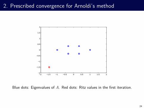
2. Prescribed convergence for Arnoldi’s method
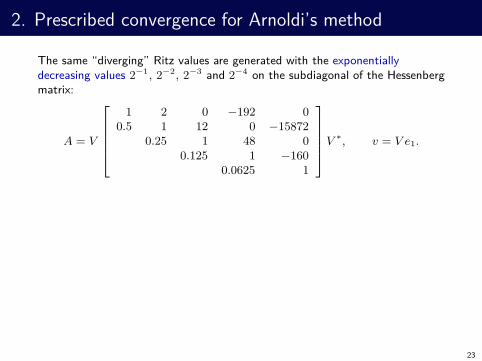
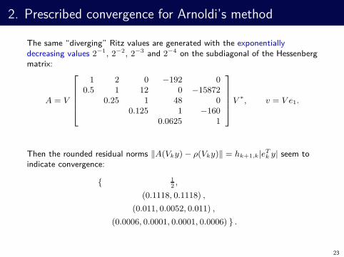
The same “diverging” Ritz values are generated with the exponentiallydecreasing values 2−1, 2−2, 2−3 and 2−4 on the subdiagonal of the Hessenbergmatrix:
A = V
1 2 0 −192 00.5 1 12 0 −15872
0.25 1 48 00.125 1 −160
0.0625 1
V ∗, v = V e1.
Then the rounded residual norms ‖A(Vky) − ρ(Vky)‖ = hk+1,k|eTk y| seem to
indicate convergence:
{ 12,
(0.1118, 0.1118) ,
(0.011, 0.0052, 0.011) ,
(0.0006, 0.0001, 0.0001, 0.0006) } .
23
2. Prescribed convergence for Arnoldi’s method
−2 −1.5 −1 −0.5 0 0.5 1 1.5 2−2
−1.5
−1
−0.5
0
0.5
1
1.5
2
Blue dots: Eigenvalues of A. Red dots: Ritz values in the first iteration.
24
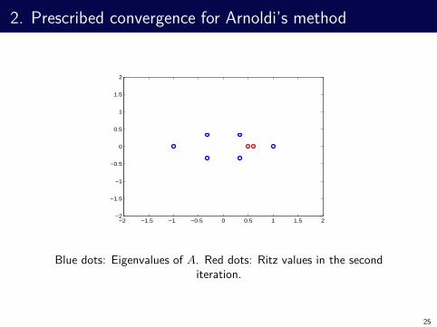
2. Prescribed convergence for Arnoldi’s method
−2 −1.5 −1 −0.5 0 0.5 1 1.5 2−2
−1.5
−1
−0.5
0
0.5
1
1.5
2
Blue dots: Eigenvalues of A. Red dots: Ritz values in the second
iteration.
25
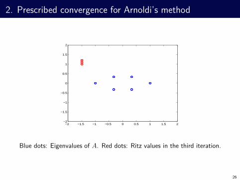
2. Prescribed convergence for Arnoldi’s method
−2 −1.5 −1 −0.5 0 0.5 1 1.5 2−2
−1.5
−1
−0.5
0
0.5
1
1.5
2
Blue dots: Eigenvalues of A. Red dots: Ritz values in the third iteration.
26
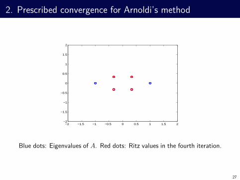
2. Prescribed convergence for Arnoldi’s method
−2 −1.5 −1 −0.5 0 0.5 1 1.5 2−2
−1.5
−1
−0.5
0
0.5
1
1.5
2
Blue dots: Eigenvalues of A. Red dots: Ritz values in the fourth iteration.
27
2. Prescribed convergence for Arnoldi’s method
−2 −1.5 −1 −0.5 0 0.5 1 1.5 2−2
−1.5
−1
−0.5
0
0.5
1
1.5
2
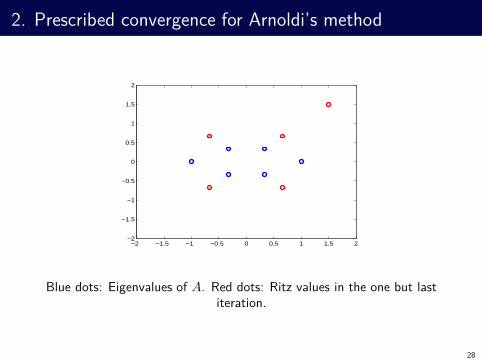
Blue dots: Eigenvalues of A. Red dots: Ritz values in the one but last
iteration.
28
2. Prescribed convergence for Arnoldi’s method
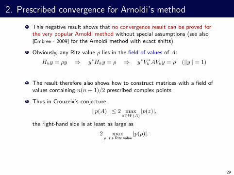
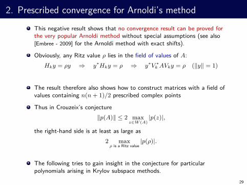
This negative result shows that no convergence result can be proved forthe very popular Arnoldi method without special assumptions (see also[Embree - 2009] for the Arnoldi method with exact shifts).
29
2. Prescribed convergence for Arnoldi’s method
This negative result shows that no convergence result can be proved forthe very popular Arnoldi method without special assumptions (see also[Embree - 2009] for the Arnoldi method with exact shifts).
Obviously, any Ritz value ρ lies in the field of values of A:
Hky = ρy ⇒ y∗Hky = ρ ⇒ y∗V ∗
k AVky = ρ (‖y‖ = 1)
The result therefore also shows how to construct matrices with a field ofvalues containing n(n + 1)/2 prescribed complex points
Thus in Crouzeix’s conjecture
‖p(A)‖ ≤ 2 maxz∈W (A)
|p(z)|,
the right-hand side is at least as large as
2 maxρ is a Ritz value
|p(ρ)|.
The following tries to gain insight in the conjecture for particularpolynomials arising in Krylov subspace methods.
29
3. Prescribed convergence for Arnoldi and GMRES
First, let us consider the GMRES polynomial.
30
3. Prescribed convergence for Arnoldi and GMRES
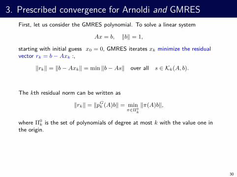
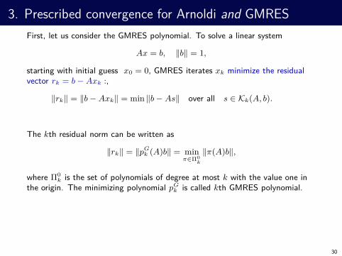
First, let us consider the GMRES polynomial. To solve a linear system
Ax = b, ‖b‖ = 1,
starting with initial guess x0 = 0, GMRES iterates xk minimize the residualvector rk = b − Axk :,
‖rk‖ = ‖b − Axk‖ = min ‖b − As‖ over all s ∈ Kk(A, b).
30
3. Prescribed convergence for Arnoldi and GMRES
First, let us consider the GMRES polynomial. To solve a linear system
Ax = b, ‖b‖ = 1,
starting with initial guess x0 = 0, GMRES iterates xk minimize the residualvector rk = b − Axk :,
‖rk‖ = ‖b − Axk‖ = min ‖b − As‖ over all s ∈ Kk(A, b).
The kth residual norm can be written as
‖rk‖ = ‖pGk (A)b‖ = min
π∈Π0
k
‖π(A)b‖,
where Π0k is the set of polynomials of degree at most k with the value one in
the origin.
30
3. Prescribed convergence for Arnoldi and GMRES
First, let us consider the GMRES polynomial. To solve a linear system
Ax = b, ‖b‖ = 1,
starting with initial guess x0 = 0, GMRES iterates xk minimize the residualvector rk = b − Axk :,
‖rk‖ = ‖b − Axk‖ = min ‖b − As‖ over all s ∈ Kk(A, b).
The kth residual norm can be written as
‖rk‖ = ‖pGk (A)b‖ = min
π∈Π0
k
‖π(A)b‖,
where Π0k is the set of polynomials of degree at most k with the value one in
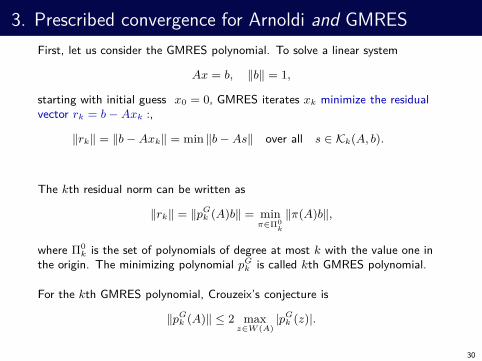
the origin. The minimizing polynomial pGk is called kth GMRES polynomial.
30
3. Prescribed convergence for Arnoldi and GMRES
First, let us consider the GMRES polynomial. To solve a linear system
Ax = b, ‖b‖ = 1,
starting with initial guess x0 = 0, GMRES iterates xk minimize the residualvector rk = b − Axk :,
‖rk‖ = ‖b − Axk‖ = min ‖b − As‖ over all s ∈ Kk(A, b).
The kth residual norm can be written as
‖rk‖ = ‖pGk (A)b‖ = min
π∈Π0
k
‖π(A)b‖,
where Π0k is the set of polynomials of degree at most k with the value one in
the origin. The minimizing polynomial pGk is called kth GMRES polynomial.
For the kth GMRES polynomial, Crouzeix’s conjecture is
‖pGk (A)‖ ≤ 2 max
z∈W (A)|pG
k (z)|.
30
3. Prescribed convergence for Arnoldi and GMRES
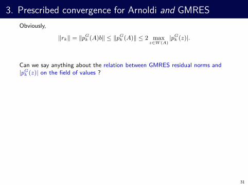
Obviously,
‖rk‖ = ‖pGk (A)b‖ ≤ ‖pG
k (A)‖ ≤ 2 maxz∈W (A)
|pGk (z)|.
31
3. Prescribed convergence for Arnoldi and GMRES
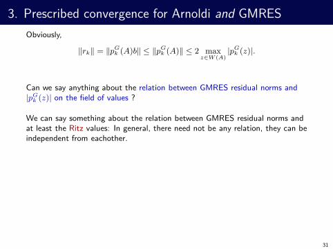
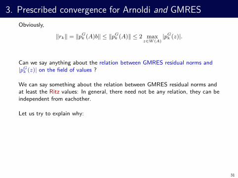
Obviously,
‖rk‖ = ‖pGk (A)b‖ ≤ ‖pG
k (A)‖ ≤ 2 maxz∈W (A)
|pGk (z)|.
Can we say anything about the relation between GMRES residual norms and|pG
k (z)| on the field of values ?
31

3. Prescribed convergence for Arnoldi and GMRES
Obviously,
‖rk‖ = ‖pGk (A)b‖ ≤ ‖pG
k (A)‖ ≤ 2 maxz∈W (A)
|pGk (z)|.
Can we say anything about the relation between GMRES residual norms and|pG
k (z)| on the field of values ?
We can say something about the relation between GMRES residual norms andat least the Ritz values:
31
3. Prescribed convergence for Arnoldi and GMRES
Obviously,
‖rk‖ = ‖pGk (A)b‖ ≤ ‖pG
k (A)‖ ≤ 2 maxz∈W (A)
|pGk (z)|.
Can we say anything about the relation between GMRES residual norms and|pG
k (z)| on the field of values ?
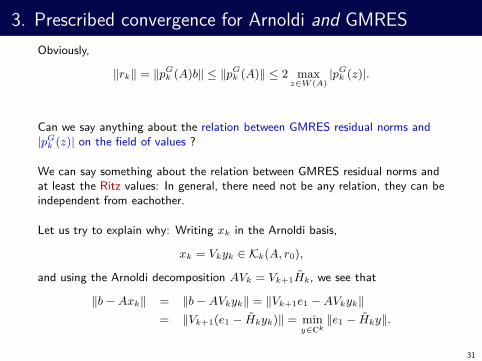
We can say something about the relation between GMRES residual norms andat least the Ritz values: In general, there need not be any relation, they can beindependent from eachother.
31
3. Prescribed convergence for Arnoldi and GMRES
Obviously,
‖rk‖ = ‖pGk (A)b‖ ≤ ‖pG
k (A)‖ ≤ 2 maxz∈W (A)
|pGk (z)|.
Can we say anything about the relation between GMRES residual norms and|pG
k (z)| on the field of values ?
We can say something about the relation between GMRES residual norms andat least the Ritz values: In general, there need not be any relation, they can beindependent from eachother.
Let us try to explain why:
31
3. Prescribed convergence for Arnoldi and GMRES
Obviously,
‖rk‖ = ‖pGk (A)b‖ ≤ ‖pG
k (A)‖ ≤ 2 maxz∈W (A)
|pGk (z)|.
Can we say anything about the relation between GMRES residual norms and|pG
k (z)| on the field of values ?
We can say something about the relation between GMRES residual norms andat least the Ritz values: In general, there need not be any relation, they can beindependent from eachother.
Let us try to explain why: Writing xk in the Arnoldi basis,
xk = Vkyk ∈ Kk(A, r0),
and using the Arnoldi decomposition AVk = Vk+1Hk, we see that
‖b − Axk‖ = ‖b − AVkyk‖ = ‖Vk+1e1 − AVkyk‖= ‖Vk+1(e1 − Hkyk)‖ = min
y∈Ck
‖e1 − Hky‖.
31
3. Prescribed convergence for Arnoldi and GMRES
Thus the residual norms generated by the GMRES method are fully determinedby the Hessenberg matrix Hk.
32
3. Prescribed convergence for Arnoldi and GMRES
Thus the residual norms generated by the GMRES method are fully determinedby the Hessenberg matrix Hk.
We have seen that the subdiagonal entries of Hk can be chosenarbitrarily, for any prescribed Ritz values in the kth iteration.
32
3. Prescribed convergence for Arnoldi and GMRES
Thus the residual norms generated by the GMRES method are fully determinedby the Hessenberg matrix Hk.
We have seen that the subdiagonal entries of Hk can be chosenarbitrarily, for any prescribed Ritz values in the kth iteration.
Hence there is a chance we can modify the behavior of GMRES whilemaintaining the prescribed Ritz values.
Example from earlier: Consider the prescribed ’diverging’ Ritz values
R = { 1,
(0, 2) ,
(−1, 1, 3) ,
(−2, 0, 2, 4) ,
(1, 1, 1, 1, 1)} ,
and the prescribed subdiagonal entries of the generated Hessenberg matrix
σ1 = 2−1, σ2 = 2−2, σ3 = 2−3, σ4 = 2−4.
32
3. Prescribed convergence for Arnoldi and GMRES
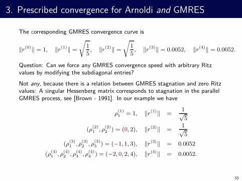
The corresponding GMRES convergence curve is
‖r(0)‖ = 1, ‖r(1)‖ =
√
1
5, ‖r(2)‖ =
√
1
5, ‖r(3)‖ = 0.0052, ‖r(4)‖ = 0.0052.
Question: Can we force any GMRES convergence speed with arbitrary Ritzvalues by modifying the subdiagonal entries?
Not any, because there is a relation between GMRES stagnation and zero Ritzvalues: A singular Hessenberg matrix corresponds to stagnation in the parallelGMRES process, see [Brown - 1991]. In our example we have
ρ(1)1 = 1, ‖r(1)‖ =
1√5
(ρ(2)1 , ρ
(2)2 ) = (0, 2), ‖r(2)‖ =
1√5
(ρ(3)1 , ρ
(3)2 , ρ
(3)3 ) = (−1, 1, 3), ‖r(3)‖ = 0.0052
(ρ(4)1 , ρ
(4)2 , ρ
(4)3 , ρ
(4)4 ) = (−2, 0, 2, 4), ‖r(4)‖ = 0.0052.
33
3. Prescribed convergence for Arnoldi and GMRES
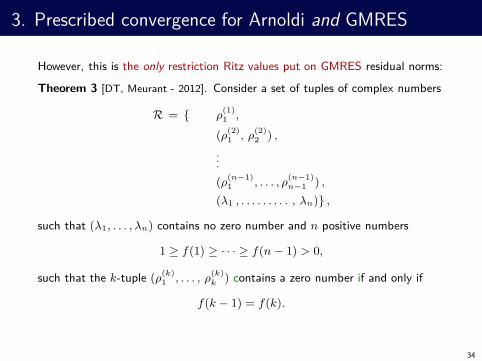
However, this is the only restriction Ritz values put on GMRES residual norms:
Theorem 3 [DT, Meurant - 2012]. Consider a set of tuples of complex numbers
R = { ρ(1)1 ,
(ρ(2)1 , ρ
(2)2 ) ,
...
(ρ(n−1)1 , . . . , ρ
(n−1)n−1 ) ,
(λ1 , . . . . . . . . . , λn)} ,
such that (λ1, . . . , λn) contains no zero number and n positive numbers
1 ≥ f(1) ≥ · · · ≥ f(n − 1) > 0,
such that the k-tuple (ρ(k)1 , . . . , ρ
(k)k ) contains a zero number if and only if
f(k − 1) = f(k).
34
3. Prescribed convergence for Arnoldi and GMRES
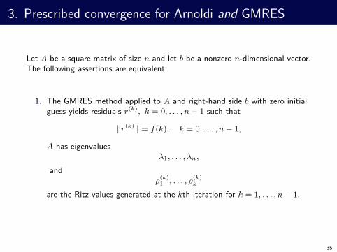
Let A be a square matrix of size n and let b be a nonzero n-dimensional vector.The following assertions are equivalent:
1. The GMRES method applied to A and right-hand side b with zero initialguess yields residuals r(k), k = 0, . . . , n − 1 such that
‖r(k)‖ = f(k), k = 0, . . . , n − 1,
A has eigenvaluesλ1, . . . , λn,
andρ
(k)1 , . . . , ρ
(k)k
are the Ritz values generated at the kth iteration for k = 1, . . . , n − 1.
35
3. Prescribed convergence for Arnoldi and GMRES
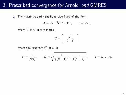
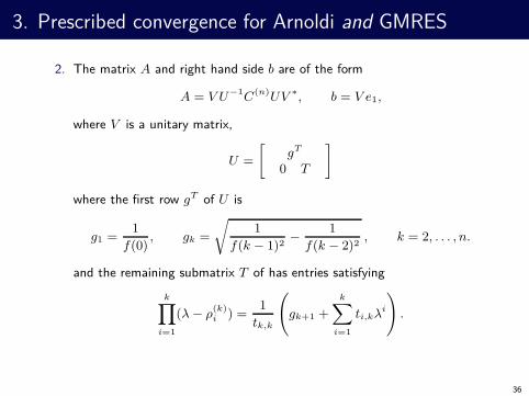
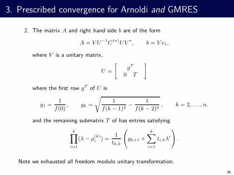
2. The matrix A and right hand side b are of the form
A = V U−1C(n)UV ∗, b = V e1,
where V is a unitary matrix,
U =
[
gT
0 T
]
where the first row gT of U is
g1 =1
f(0), gk =
√
1
f(k − 1)2− 1
f(k − 2)2, k = 2, . . . , n.
36
3. Prescribed convergence for Arnoldi and GMRES
2. The matrix A and right hand side b are of the form
A = V U−1C(n)UV ∗, b = V e1,
where V is a unitary matrix,
U =
[
gT
0 T
]
where the first row gT of U is
g1 =1
f(0), gk =
√
1
f(k − 1)2− 1
f(k − 2)2, k = 2, . . . , n.
and the remaining submatrix T of has entries satisfying
k∏
i=1
(λ − ρ(k)i ) =
1
tk,k
(
gk+1 +
k∑
i=1
ti,kλi
)
.
Note we exhausted all freedom modulo unitary transformation.
36
3. Prescribed convergence for Arnoldi and GMRES
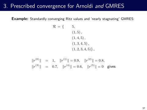
Example: Standardly converging Ritz values and ’nearly stagnating’ GMRES:
R = { 5,
(1, 5) ,
(1, 4, 5) ,
(1, 3, 4, 5) ,
(1, 2, 3, 4, 5)} ,
‖r(0)‖ = 1, ‖r(1)‖ = 0.9, ‖r(2)‖ = 0.8,
‖r(3)‖ = 0.7, ‖r(4)‖ = 0.6, ‖r(5)‖ = 0 gives
37
3. Prescribed convergence for Arnoldi and GMRES
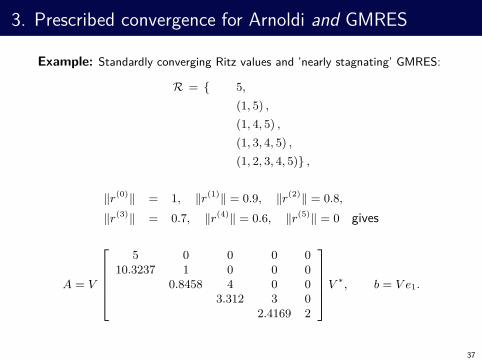
Example: Standardly converging Ritz values and ’nearly stagnating’ GMRES:
R = { 5,
(1, 5) ,
(1, 4, 5) ,
(1, 3, 4, 5) ,
(1, 2, 3, 4, 5)} ,
‖r(0)‖ = 1, ‖r(1)‖ = 0.9, ‖r(2)‖ = 0.8,
‖r(3)‖ = 0.7, ‖r(4)‖ = 0.6, ‖r(5)‖ = 0 gives
A = V
5 0 0 0 010.3237 1 0 0 0
0.8458 4 0 03.312 3 0
2.4169 2
V ∗, b = V e1.
37
3. Prescribed convergence for Arnoldi and GMRES
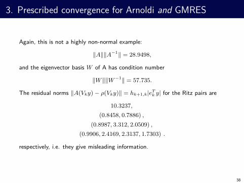
Again, this is not a highly non-normal example:
‖A‖‖A−1‖ = 28.9498,
and the eigenvector basis W of A has condition number
‖W ‖‖W −1‖ = 57.735.
The residual norms ‖A(Vky) − ρ(Vky)‖ = hk+1,k|eTk y| for the Ritz pairs are
10.3237,
(0.8458, 0.7886) ,
(0.8987, 3.312, 2.0509) ,
(0.9906, 2.4169, 2.3137, 1.7303) .
respectively, i.e. they give misleading information.
38
3. Prescribed convergence for Arnoldi and GMRES
Summarizing, any GMRES residual norms are possible with any Ritz values inall iterations.
39
3. Prescribed convergence for Arnoldi and GMRES
Summarizing, any GMRES residual norms are possible with any Ritz values inall iterations.
We have proved two more analogue results:
Any GMRES residual norms are possible with any harmonic Ritz values inall iterations.
39
3. Prescribed convergence for Arnoldi and GMRES
Summarizing, any GMRES residual norms are possible with any Ritz values inall iterations.
We have proved two more analogue results:
Any GMRES residual norms are possible with any harmonic Ritz values inall iterations. This is perhaps even more surprising, because the harmonicRitz values are the roots of GMRES polynomials.
39
3. Prescribed convergence for Arnoldi and GMRES
Summarizing, any GMRES residual norms are possible with any Ritz values inall iterations.
We have proved two more analogue results:
Any GMRES residual norms are possible with any harmonic Ritz values inall iterations. This is perhaps even more surprising, because the harmonicRitz values are the roots of GMRES polynomials. However, harmonic Ritzvalues are not in general in the field of values of A, so this has noimplications for Crouzeix’s conjecture for the GMRES polynomial.
Any FOM residual norms are possible with any Ritz values in all iterations.
The FOM method differs from the GMRES method in that the residual norm isnot minimized, but the kth FOM residual vector is characterized through
rFk ⊥ Kk(A, b).
39
3. Prescribed convergence for Arnoldi and GMRES
The corresponding residual norms are related through to formula
1
‖rFk ‖ =
√
1
‖rGk ‖2
− 1
‖rGk−1‖2
.
Note that FOM residual norms need not be non-increasing and are not definedif the corresponding GMRES iterate stagnates.
40
3. Prescribed convergence for Arnoldi and GMRES
The corresponding residual norms are related through to formula
1
‖rFk ‖ =
√
1
‖rGk ‖2
− 1
‖rGk−1‖2
.
Note that FOM residual norms need not be non-increasing and are not definedif the corresponding GMRES iterate stagnates.
What seems interesting to me in the context of the Crouzeix’s conjecture isthat the Ritz values are the roots of the FOM polynomials:
FOM polynomials might lead to a way to test if the conjecture can bedisproved. For the kth FOM polynomial pF
k we have,
0 = 2 maxρ is a Ritz value
|pFk (ρ)| < ‖rF
k ‖ = ‖pFk (A)b‖ ≤ ‖pF
k (A)‖.
Note the residual norms can be chosen arbitrarely large...
The construction to prescribe Ritz values and FOM residual norms is thefollowing:
40

3. Prescribed convergence for Arnoldi and GMRES
The matrix A and right hand side b are of the form
A = V U−1C(n)UV ∗, b = V e1,
where V is a unitary matrix,
U =
[
gT
0 T
]
where to force FOM residual norms f(0), . . . , f(n − 1), f(i) > 0, the first rowgT of U can be chosen as
gk =1
f(k − 1), k = 1, . . . , n
and the remaining submatrix T of has entries satisfying
k∏
i=1
(λ − ρ(k)i ) =
1
tk,k
(
gk+1 +
k∑
i=1
ti,kλi
)
.
41

Thank you for your attention.
42
Related publications
A. Greenbaum, V. Pták and Z. Strakoš, Any nonincreasing convergence curve is possible for GMRES,
SIAM J. Matrix Anal. Appl., 17 (1996), pp. 465–469.
M. Arioli, V. Pták and Z. Strakoš, Krylov sequences of maximal length and convergence of GMRES, BIT
Num. Maths., 38 (1996), pp. 636–643.
J. Duintjer Tebbens and G. Meurant, Any Ritz value behavior is possible for Arnoldi and for GMRES,
SIAM J. Matrix Anal. Appl., 33 (2012), pp. 958–978.
J. Duintjer Tebbens and G. Meurant, Prescribing the behavior of early terminating GMRES and Arnoldi
iterations, Numer. Algorithms, 65 (2014), pp. 69–90.
J. Duintjer Tebbens, G. Meurant, H. Sadok and Z. Strakoš, On investigating GMRES convergence using
unitary matrices, Lin. Alg. Appl., 450 (2014), pp. 83–107.
G. Meurant and J. Duintjer Tebbens, The role eigenvalues play in forming GMRES residual norms with
non-normal matrices, Numer. Algorithms, 68 (2015), pp. 143–165.
J. Duintjer Tebbens and G. Meurant, On the convergence of QOR and QMR Krylov methods for solving
nonsymmetric linear systems, BIT Num. Maths., 56 (2016), pp. 77–97.
43