On a numerical subgrid upscaling algorithm for

Stokes–Brinkman equations

O. Ilieva, Z. Lakdawalaa, V. Starikoviciusb

aFraunhofer ITWM, Fraunhofer-Platz 1, D-67663 Kaiserslautern, Germanyiliev, lakdawala@itwm.fhg.de

bVilnius Gediminas Technical University, Vilnius, Lithuaniavadimas.starikovicius@sc.vgtu.lt

Abstract

This paper discusses a numerical subgrid resolution approach for solving theStokes-Brinkman system of equations, which is describing coupled flow inplain and in highly porous media. Various scientific and industrial problemsare described by this system, and often the geometry and/or the permeabil-ity vary on several scales. A particular target is the process of oil filtration.In many complicated filters, the filter medium or the filter element geometryare too fine to be resolved by a feasible computational grid. The subgridapproach presented in the paper is aimed at describing how these fine detailsare accounted for by solving auxiliary problems in appropriately chosen gridcells on a relatively coarse computational grid. This is done via a systematicand a careful procedure of modifying and updating the coefficients of theStokes-Brinkman system in chosen cells. This numerical subgrid approachis motivated from one side from homogenization theory, from which we bor-row the formulations for the so called cell problem, and from the other sidefrom the numerical upscaling approaches, such as Multiscale Finite Volume,Multiscale Finite Element, etc. Results on the algorithm’s efficiency, bothin terms of computational time and memory usage, are presented. Compari-son with solutions on full fine grid (when possible) are presented in order toevaluate the accuracy. Advantages and limitations of the considered subgridapproach are discussed.

Keywords: Stokes-Brinkman equations, subgrid approach, multiscaleproblems, numerical upscaling.

Preprint submitted to Elsevier July 4, 2010

1. Introduction

The demands of the industry regularly pose new challenging problems to ap-plied mathematics. In many cases the existing algorithms do not work, andnew specialized algorithms for classes of industrial problems are demanded.Developing algorithms for a class of filtration problems (filtering solid par-ticles out of liquid) is discussed in this paper. Numerical simulations, whenthey can be performed, allow significant reduction in time and costs for de-sign of new filter elements with proper flow rate - pressure drop ratio. TheCFD simulations assisting this design are characterized by three peculiarities:

• The filtering porous layers are usually manufactured with certain varia-tions in the weight (i.e., in porosity and permeability), and consistentlywith this, accuracy of 5 to 8 per cent for the pressure drop across a filterelement is the target of the simulations.

• High accuracy for the flow velocity within a filter element is not re-quired, as long as the pressure drop over the complete filter element isproperly computed.

• 30-36 simulations with different flow rates and different viscosities haveto be performed for each geometry to evaluate the performance of thefilter element at different flow and temperature conditions.

Our aim is to account for these peculiarities, in order to develop efficientalgorithm for this particular class of problems.In the case of liquid filtration, the flow is usually laminar, and at low andmoderate temperatures it is slow (due to higher viscosity), and it is describedby the Stokes-Brinkman system of equations (see, e.g., [22] and referencestherein):

ρ∂~u

∂t−∇ · (µ∇~u)︸ ︷︷ ︸

Stokes

+

Darcy︷ ︸︸ ︷µK

−1~u+∇p = ~f︸ ︷︷ ︸ (1)

∇ · ~u = 0,

where

µ =

µ in Ωf

µeff in Ωp

~f =

~fNS in Ωf

~fB in Ωp

K−1

=

0 in Ωf

K−1 in Ωp

2

Here ~u, p stand for velocity and pressure respectively, ρ, µ and K denotethe density, viscosity, and the permeability tensor of the porous medium,respectively.

The Stokes equations (cf. [4, 19]) govern the flow in pure fluid regions. TheBrinkman equations (cf. [7]) are introduced as an extension to the Darcymodel for the flow in porous media for the case of highly porous media (note,that porosity of the non-woven filtering media, which is our primary interest,is often more than 0.9). Concerning the hierarchy of the models for theporous media flow, we refer to the recent review in [10]. The Stokes-Brinkmansystem is used to describe the coupled flow in plain and in porous media. Forits justification, see [18]. Some details on modeling and simulation of flowthrough oil filters using the Stokes-Brinkman and Navier-Stokes-Brinkmansystems of equations can be found in [30, 15, 22].

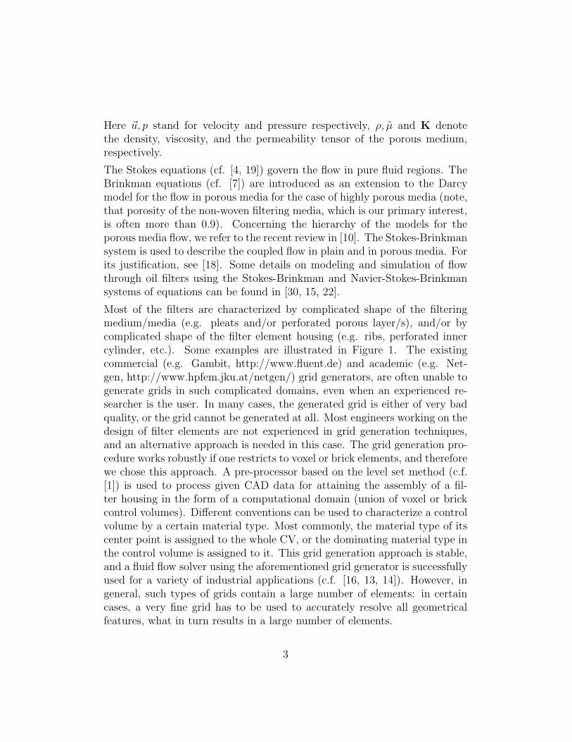
Most of the filters are characterized by complicated shape of the filteringmedium/media (e.g. pleats and/or perforated porous layer/s), and/or bycomplicated shape of the filter element housing (e.g. ribs, perforated innercylinder, etc.). Some examples are illustrated in Figure 1. The existingcommercial (e.g. Gambit, http://www.fluent.de) and academic (e.g. Net-gen, http://www.hpfem.jku.at/netgen/) grid generators, are often unable togenerate grids in such complicated domains, even when an experienced re-searcher is the user. In many cases, the generated grid is either of very badquality, or the grid cannot be generated at all. Most engineers working on thedesign of filter elements are not experienced in grid generation techniques,and an alternative approach is needed in this case. The grid generation pro-cedure works robustly if one restricts to voxel or brick elements, and thereforewe chose this approach. A pre-processor based on the level set method (c.f.[1]) is used to process given CAD data for attaining the assembly of a fil-ter housing in the form of a computational domain (union of voxel or brickcontrol volumes). Different conventions can be used to characterize a controlvolume by a certain material type. Most commonly, the material type of itscenter point is assigned to the whole CV, or the dominating material type inthe control volume is assigned to it. This grid generation approach is stable,and a fluid flow solver using the aforementioned grid generator is successfullyused for a variety of industrial applications (c.f. [16, 13, 14]). However, ingeneral, such types of grids contain a large number of elements: in certaincases, a very fine grid has to be used to accurately resolve all geometricalfeatures, what in turn results in a large number of elements.

3

Figure 1: Some examples of the complex geometries and complicated shapes of the filteringmedia.

For the cases where the geometrical features are at different scales, variousapproaches for multiscale problems can be adopted to provide an increasein the efficiency of the flow algorithms. Recall that the Darcy equation canbe rigorously derived as a macroscopic model for flow in porous media, inthe case of periodic or statistically homogeneous porous media. The Stokessystem of equations at pore scale (c.f. [27]) is the basis of these derivations.Depending on the the porosity, Allaire [6] homogenizes the Stokes problem tothe Darcy or the Brinkman system. Clearly, the homogenization approach isvery restrictive, i.e. it can be used only for periodic or statistically homoge-neous porous media, and for the Stokes (and not for Navier-Stokes) systemat the pore scale. The homogenization theory works in the case of scaleseparation, and it allows for a drastic reduction of the computational costs:only one auxiliary problem is solved in a periodicity cell on the fine scale,its solution is post-processed to compute the coefficients of the macroscopicequation, and the macroscopic equation is further solved at the coarse scale.The coefficients of the macroscopic equation in this case are called upscaled,homogenized, or effective coefficients. For the cases when the homogeniza-tion theory does not work, its ideas can still be imported to the numericalupscaling approaches, such as the Multiscale Finite Element Method (Ms-FEM) [23], the Mixed MsFEM, [3], the Multiscale Finite Volume Method[21, 8, 5] and the Subgrid Method [26, 24, 9, 17]. Another approach whichserves as a building block for numerical upscaling procedures, is the volumeaveraging approach combined with the Representative Elementary Volume(REV) concept (cf. [12]). Unlike the homogenization theory, this approachis not based on asymptotic expansions, but on the volumetric averaging offunctions and their derivatives. For example, if a block of porous medium islarge enough (i.e. representative), its Darcy permeability is defined from the

4

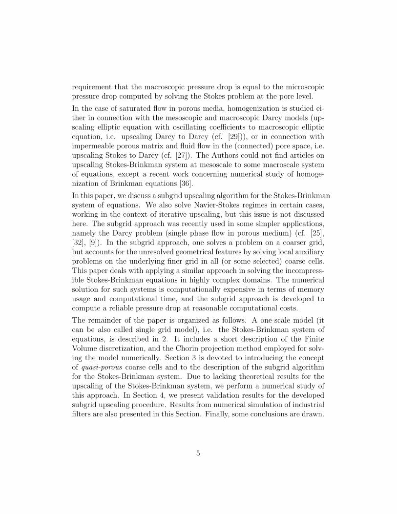
requirement that the macroscopic pressure drop is equal to the microscopicpressure drop computed by solving the Stokes problem at the pore level.

In the case of saturated flow in porous media, homogenization is studied ei-ther in connection with the mesoscopic and macroscopic Darcy models (up-scaling elliptic equation with oscillating coefficients to macroscopic ellipticequation, i.e. upscaling Darcy to Darcy (cf. [29])), or in connection withimpermeable porous matrix and fluid flow in the (connected) pore space, i.e.upscaling Stokes to Darcy (cf. [27]). The Authors could not find articles onupscaling Stokes-Brinkman system at mesoscale to some macroscale systemof equations, except a recent work concerning numerical study of homoge-nization of Brinkman equations [36].

In this paper, we discuss a subgrid upscaling algorithm for the Stokes-Brinkmansystem of equations. We also solve Navier-Stokes regimes in certain cases,working in the context of iterative upscaling, but this issue is not discussedhere. The subgrid approach was recently used in some simpler applications,namely the Darcy problem (single phase flow in porous medium) (cf. [25],[32], [9]). In the subgrid approach, one solves a problem on a coarser grid,but accounts for the unresolved geometrical features by solving local auxiliaryproblems on the underlying finer grid in all (or some selected) coarse cells.This paper deals with applying a similar approach in solving the incompress-ible Stokes-Brinkman equations in highly complex domains. The numericalsolution for such systems is computationally expensive in terms of memoryusage and computational time, and the subgrid approach is developed tocompute a reliable pressure drop at reasonable computational costs.

The remainder of the paper is organized as follows. A one-scale model (itcan be also called single grid model), i.e. the Stokes-Brinkman system ofequations, is described in 2. It includes a short description of the FiniteVolume discretization, and the Chorin projection method employed for solv-ing the model numerically. Section 3 is devoted to introducing the conceptof quasi-porous coarse cells and to the description of the subgrid algorithmfor the Stokes-Brinkman system. Due to lacking theoretical results for theupscaling of the Stokes-Brinkman system, we perform a numerical study ofthis approach. In Section 4, we present validation results for the developedsubgrid upscaling procedure. Results from numerical simulation of industrialfilters are also presented in this Section. Finally, some conclusions are drawn.

5

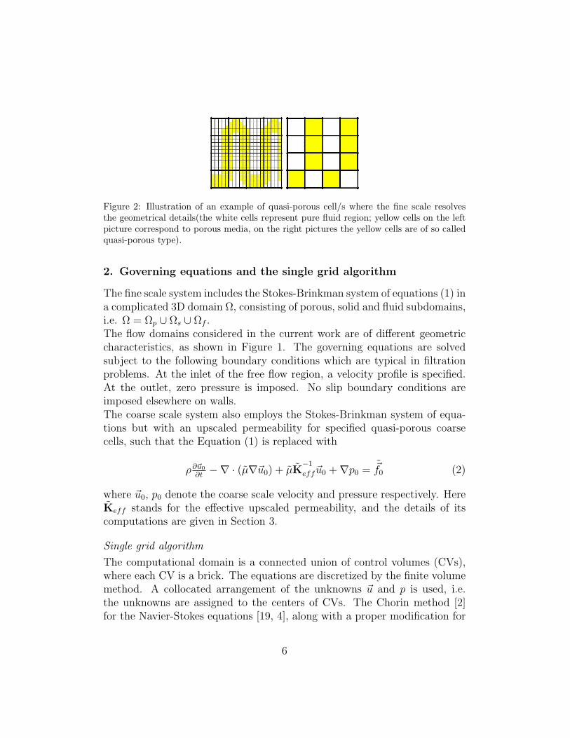
Figure 2: Illustration of an example of quasi-porous cell/s where the fine scale resolvesthe geometrical details(the white cells represent pure fluid region; yellow cells on the leftpicture correspond to porous media, on the right pictures the yellow cells are of so calledquasi-porous type).

2. Governing equations and the single grid algorithm

The fine scale system includes the Stokes-Brinkman system of equations (1) ina complicated 3D domain Ω, consisting of porous, solid and fluid subdomains,i.e. Ω = Ωp ∪ Ωs ∪ Ωf .The flow domains considered in the current work are of different geometriccharacteristics, as shown in Figure 1. The governing equations are solvedsubject to the following boundary conditions which are typical in filtrationproblems. At the inlet of the free flow region, a velocity profile is specified.At the outlet, zero pressure is imposed. No slip boundary conditions areimposed elsewhere on walls.The coarse scale system also employs the Stokes-Brinkman system of equa-tions but with an upscaled permeability for specified quasi-porous coarsecells, such that the Equation (1) is replaced with

ρ∂~u0

∂t−∇ · (µ∇~u0) + µK

−1

eff~u0 +∇p0 = ~f0 (2)

where ~u0, p0 denote the coarse scale velocity and pressure respectively. HereKeff stands for the effective upscaled permeability, and the details of itscomputations are given in Section 3.

Single grid algorithm

The computational domain is a connected union of control volumes (CVs),where each CV is a brick. The equations are discretized by the finite volumemethod. A collocated arrangement of the unknowns ~u and p is used, i.e.the unknowns are assigned to the centers of CVs. The Chorin method [2]for the Navier-Stokes equations [19, 4], along with a proper modification for

6

Stokes-Brinkman case [22], is used as a projection method decoupling velocityand continuity equations (note, the Chorin projection for unsteady Stokesproblem is very close to the preconditioners for unsteady Stokes problemsuggested in [35]) . The fractional time step discretization scheme can bewritten as

(ρ~u∗ − ρ~un) + τ(−D +B)~u∗ = τGpn (3)(ρ~un+1 − ρ~u∗

)+ τ(B~un+1 −B~u∗) = τ(Gpn+1 −Gpn) (4)

GTρ~un+1 = 0 (5)

where D~u denote the operator corresponding to the discretized viscous terms.The particular form of these operators depend on the spatial discretizations.G and GT denote the discretized gradient and divergence operator. B~u de-notes the Darcy operator in the momentum equations whereas the superscriptk+1 and k denotes the new and the old time level, respectively.

The sum of Equations (3) and (4) results in an implicit discretization of themomentum equations. Equation (3) is solved with respect to the velocitiesusing the old value of the pressure gradient, thus obtaining a prediction forthe velocity. To solve the second equation for pressure correction, one takesthe divergence from it and uses the continuity equation. The resulting equa-tion is a Poisson type equation for the pressure correction which is discussedin detail in [22].

3. Subgrid Algorithm

In this section, a subgrid algorithm for the Stokes-Brinkman system is dis-cussed. The goal is to develop an algorithm which computes not only thepressure drop across a filter element on a relatively coarse grid, but also pre-serves the pressure drop accuracy corresponding to a finer grid. The ideais to account for a subgrid resolution on the coarse grid by solving properlocal auxiliary problems on the fine grid, and using their solution for cal-culating the permeability of quasi-porous coarse cells. In fact, solving localproblems in order to account for the fine scale features is a common approachfor numerical upscaling methods, such as MsFEM, MSFV, etc.

For a given computational domain, Ω, we consider a fine grid and a coarsegrid. The fine grid is assumed to contain all important geometrical details,

7

but solving the Stokes-Brinkman system of equations on this grid is memoryand CPU intensive, or even impossible. As discussed in the Introduction, amaterial type (in our case fluid, solid, or porous) is assigned to each fine gridcell during the pre-processing stage. The coarse grid has a size, such thatthe problem is solvable at acceptable computational costs. Each coarse cellis a union of fine grid cells. Each coarse cell is considered, and the coarsegrid cells containing mixture of solid & liquid, or liquid & porous, or solid& porous, or solid & liquid & porous fine grid cells, are defined as quasi-porous cells, for which effective (upscaled) permeability tensors have to becomputed. It is assumed that the Stokes-Brinkman equations describe theflow on the fine grid and on the coarse grid. In the latter case, the coarse scalepermeability is the effective (upscaled) permeability tensor Keff . Currently,the diagonal permeability tensor i.e. Keff = K11, K22, K33 is considered,and the extension to the full tensor is ongoing work.

The computation of upscaled coefficients requires solving the local fine scaleproblem in some coarse grid cells. Two approaches are considered:

• The upscaled (effective) permeability is computed for each individualquasi-porous coarse grid cell. Similar to the block-permeability up-scaling procedure for single phase flow in porous media (cf. [31]), thelocalization boundary conditions are specified on its boundary (see dis-cussion below for more details; possible oversampling is also discussedbelow);

• Alternatively, certain union of coarse cells is considered as a singleblock for which auxiliary problem is solved on the underlying fine grid.Thereafter, the upscaled (effective) permeability is assigned to each ofthe coarse cells forming the block. This approach is motivated by theRepresentative Elementary Volume concept, where a reasonably largeheterogeneous (at a fine scale) volume has to be considered, in orderto assign effective (upscaled) coarse scale properties to it.

The upscaling approach considered here is similar to the one used by Durlof-sky et al.[11] for the elliptic pressure equation, and to the approach consideredand justified in the recent article [36]. The Darcy law is used there to computethe effective (upscaled) permeability of a coarse cell from the averaged finegrid pressure and velocity. In general, different types of (localization) bound-ary conditions can be specified for the auxiliary problems. Periodic boundaryconditions suit very well for periodic geometries. The pressure drop in one

8

of the directions, and no flow (or symmetry) in the remaining directions, areoften used. In the homogenization approach considered in [6], the constantvelocity at infinity is prescribed as the boundary condition for the auxiliaryproblem. It is well known that the choice of the localization boundary con-ditions plays an important role in numerical upscaling methods, and we arecurrently working on comparing results for different (localization) boundaryconditions. This work, however, will be reported elsewhere. Currently, thefollowing local boundary conditions are considered for the auxiliary problemsfor the Stokes-Brinkman system:

• inflow velocity Uin at the inlet face (for the current direction);

• outflow b.c. at the outlet face: p = Pout,∂u∂n

= 0;

• symmetry b.c. elsewhere.

The auxiliary problems are solved for each direction d. Next, the averageinlet pressure Pin is computed from the local fine scale solution and is usedto obtain the effective permeability Kdd of the quasi-porous cell in directiond from the Darcy law [12, 36]:

Kdd =µUinLd

Pin − Pout

, (6)

where Ld is the distance between the inlet and outlet faces. The use of thisapproach is motivated by the fact that we are interested in computing theaccurate pressure drop of the complete filter element. By calculating theeffective permeability using Equation (6), we account for the resistance ofthe geometrical features which were otherwise unresolved on the coarse com-putational grid. Note, that in [36], this approach for computing the effectivepermeability was carefully and systematically compared to the standard for-mula from the homogenization literature (e.g., [6, 27]), and a very goodagreement was found.

Implementation of the subgrid method

Here, we discuss the Subgrid method. The algorithm consists of four maincomponents:

1. Selection of the quasi-porous coarse cells

9

2. Solution of the auxiliary problems with a fine grid resolution on selectedcoarse cells with boundary conditions, as specified above

3. Computation of the effective permeabilities for the quasi-porous cells

4. Solution of the full coarse scale problem, using the calculated effectivepermeabilities.

Step (1) includes a mapping of each coarse cell onto the underlying unionof fine grid cells. If the composition of fine grid cells contains a mixtureof fluid and/or porous and/or solid, it is marked with a ’quasi-porous’ flag.Alternatively, at this stage, a block of coarse cell can be specified as quasi-porous.

Step (2) defines the local auxiliary problem on the quasi-porous coarse cells.The same space discretization, i.e. the finite-volume method, is consideredon the fine scale and a solution is computed. Note, that additional layers canbe added to a quasi-porous cell. In upscaling techniques, this is known asoversampling. Mostly, the domain is extended by a ’bordering ring’ with finegrid cells. We consider additional fine scale ’bordering layers’ of type ’fluid’on a specified boundary. The number of additional layers is denoted by l inthe next section. If l = 0, it is a purely local auxiliary solve. If l = 1, itmeans that the auxiliary problem is solved in coarse cell extended with onefluid layer in the specified direction, as shown on Figure 5(d).

Step (3) assigns the effective permeability tensors to the coarse cells, post-processing the auxiliary fine grid solution computed from step (2). Steps (2)and (3) are performed for every quasi-porous cell selected in step (1). Note,that in the case when the coarse cells/blocks are periodic (e.g., this is thecase when each coarse quasi-porous block contains one pleat), the auxiliaryproblem needs to be solved once for each type of quasi-porous coarse cells.Furthermore, the once computed permeabilities are reused in the compu-tations with the same geometry, but with a different flow rate or viscosity(recall that 30-36 simulations have to be performed for each filter elementgeometry).

Step (4) includes the standard algorithm which solves the Stokes-Brinkmansystem of equations on the coarse grid.

Remark 1 : (1) The same solver is used for solving global coarse scale problemand auxiliary problems on the fine grid. (2) Different stopping criteria canbe specified for the local and for the global problems.

10

Remark 2: If the number of quasi-porous blocks is too large, Steps (2)-(3)become the most time consuming part of the solution procedure. Implemen-tation is modular-based and the subgrid algorithm is parallelized, so that theauxiliary problems are distributed to different processes for faster computa-tions.

4. Results and validation

The results from numerical simulations are presented in this section. Theperformed simulations can be divided into three groups:

• Validation for thin porous layer and for the upscaled permeability com-putation (Subsections 4.1 and 4.2). Stokes flow around a spherical ob-stacle is considered in the Subsection 4.1 to check the influence of theused voxel grid as well;

• Numerical study of Brinkman to Brinkman upscaling. As mentionedearlier, the upscaling approaches for Stokes and for Darcy flows aretheoretically considered in the literature, and due to the lack of the-oretical results for the upscaling of Brinkman equation, we perform anumerical study here (we refer also to the recent paper [36]);

• Simulations for the industrial filters with complicated geometry of theporous media (perforated layer in one case, pleats in the other case),and complicated geometry (solid mesh supporting the perforated layerin one case, and complicated filter element housing in the other case).

Whenever possible, the results from the simulations with the upscaled equa-tions are compared with the results obtained solving the fine grid problemfor the same geometry. This is the methodology employed for the validationof the developed subgrid algorithm. It should be noted that the single gridsimulations have already been validated against measurements(c.f. [30]).

The computations and CPU time measurements were performed on dedicatednode of Fraunhofer ITWM cluster ’Hercules’ with dual Intel Xeon 5148LV(’Woodcrest’) processor (2.33 GHz).

4.1. Permeability for a periodicity cell: flow around a sphere

For better understanding of the subgrid algorithm, an example of an auxil-iary problem for a quasi-porous coarse cell is considered. Consider a cube

11

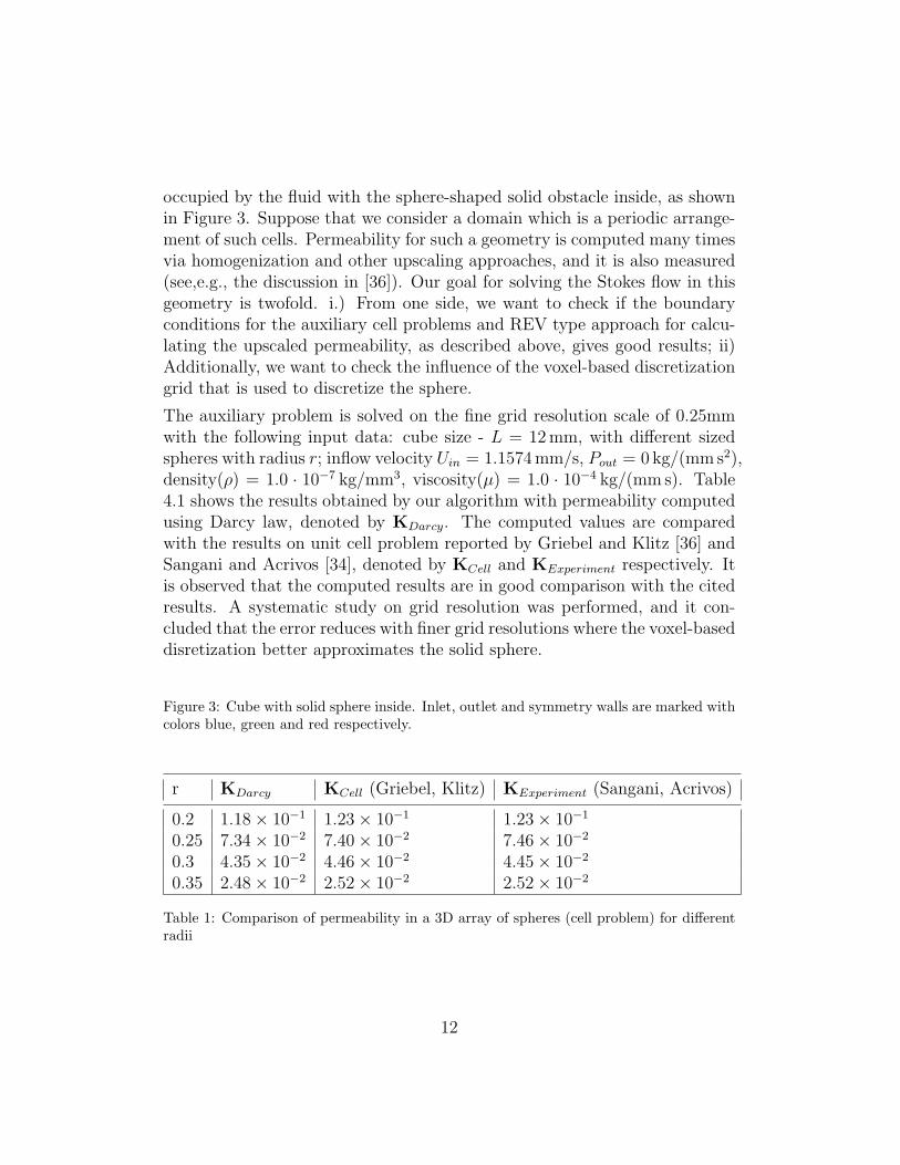
occupied by the fluid with the sphere-shaped solid obstacle inside, as shownin Figure 3. Suppose that we consider a domain which is a periodic arrange-ment of such cells. Permeability for such a geometry is computed many timesvia homogenization and other upscaling approaches, and it is also measured(see,e.g., the discussion in [36]). Our goal for solving the Stokes flow in thisgeometry is twofold. i.) From one side, we want to check if the boundaryconditions for the auxiliary cell problems and REV type approach for calcu-lating the upscaled permeability, as described above, gives good results; ii)Additionally, we want to check the influence of the voxel-based discretizationgrid that is used to discretize the sphere.

The auxiliary problem is solved on the fine grid resolution scale of 0.25mmwith the following input data: cube size - L = 12 mm, with different sizedspheres with radius r; inflow velocity Uin = 1.1574 mm/s, Pout = 0 kg/(mm s2),density(ρ) = 1.0 · 10−7 kg/mm3, viscosity(µ) = 1.0 · 10−4 kg/(mm s). Table4.1 shows the results obtained by our algorithm with permeability computedusing Darcy law, denoted by KDarcy. The computed values are comparedwith the results on unit cell problem reported by Griebel and Klitz [36] andSangani and Acrivos [34], denoted by KCell and KExperiment respectively. Itis observed that the computed results are in good comparison with the citedresults. A systematic study on grid resolution was performed, and it con-cluded that the error reduces with finer grid resolutions where the voxel-baseddisretization better approximates the solid sphere.

Figure 3: Cube with solid sphere inside. Inlet, outlet and symmetry walls are marked withcolors blue, green and red respectively.

r KDarcy KCell (Griebel, Klitz) KExperiment (Sangani, Acrivos)

0.2 1.18× 10−1 1.23× 10−1 1.23× 10−1

0.25 7.34× 10−2 7.40× 10−2 7.46× 10−2

0.3 4.35× 10−2 4.46× 10−2 4.45× 10−2

0.35 2.48× 10−2 2.52× 10−2 2.52× 10−2

Table 1: Comparison of permeability in a 3D array of spheres (cell problem) for differentradii

12

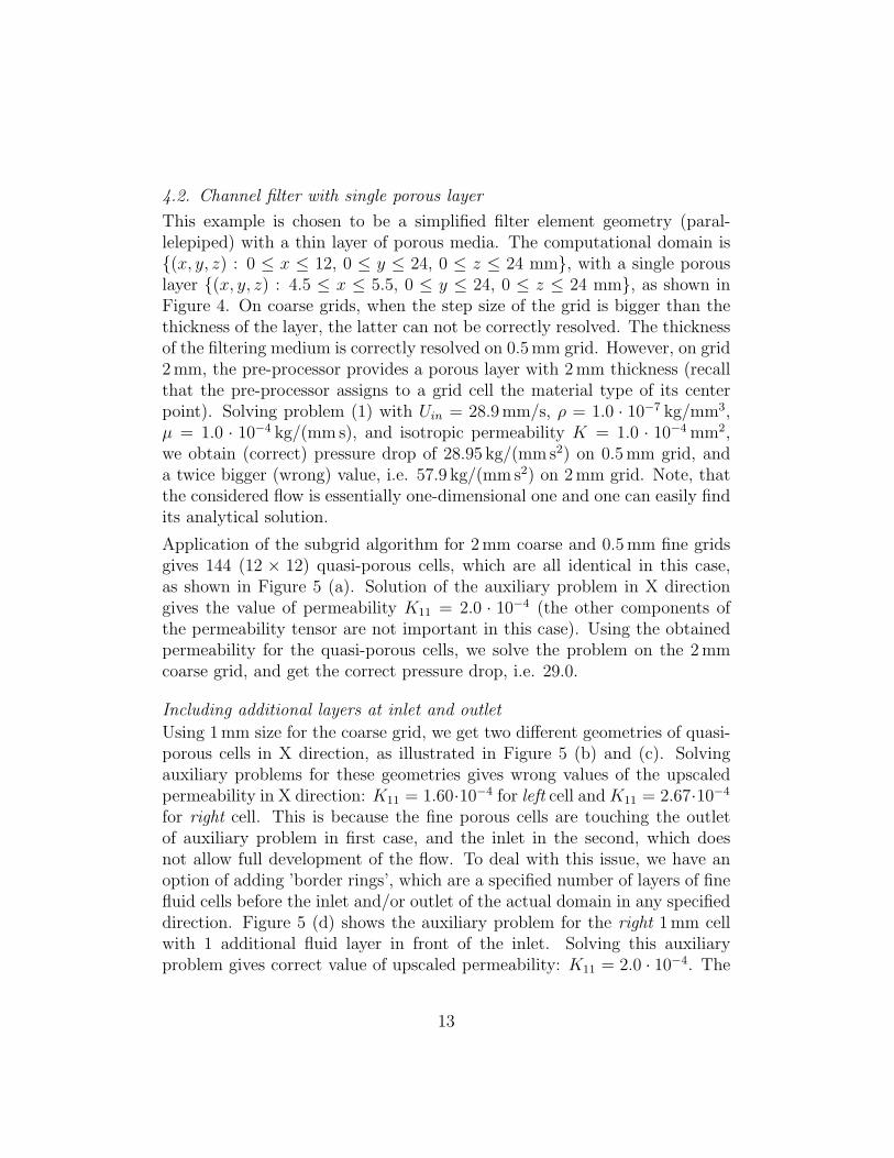
4.2. Channel filter with single porous layer

This example is chosen to be a simplified filter element geometry (paral-lelepiped) with a thin layer of porous media. The computational domain is(x, y, z) : 0 ≤ x ≤ 12, 0 ≤ y ≤ 24, 0 ≤ z ≤ 24 mm, with a single porouslayer (x, y, z) : 4.5 ≤ x ≤ 5.5, 0 ≤ y ≤ 24, 0 ≤ z ≤ 24 mm, as shown inFigure 4. On coarse grids, when the step size of the grid is bigger than thethickness of the layer, the latter can not be correctly resolved. The thicknessof the filtering medium is correctly resolved on 0.5 mm grid. However, on grid2 mm, the pre-processor provides a porous layer with 2 mm thickness (recallthat the pre-processor assigns to a grid cell the material type of its centerpoint). Solving problem (1) with Uin = 28.9 mm/s, ρ = 1.0 · 10−7 kg/mm3,µ = 1.0 · 10−4 kg/(mm s), and isotropic permeability K = 1.0 · 10−4 mm2,we obtain (correct) pressure drop of 28.95 kg/(mm s2) on 0.5 mm grid, anda twice bigger (wrong) value, i.e. 57.9 kg/(mm s2) on 2 mm grid. Note, thatthe considered flow is essentially one-dimensional one and one can easily findits analytical solution.

Application of the subgrid algorithm for 2 mm coarse and 0.5 mm fine gridsgives 144 (12 × 12) quasi-porous cells, which are all identical in this case,as shown in Figure 5 (a). Solution of the auxiliary problem in X directiongives the value of permeability K11 = 2.0 · 10−4 (the other components ofthe permeability tensor are not important in this case). Using the obtainedpermeability for the quasi-porous cells, we solve the problem on the 2 mmcoarse grid, and get the correct pressure drop, i.e. 29.0.

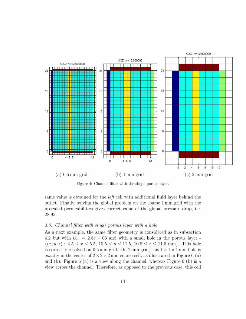
Including additional layers at inlet and outlet

Using 1 mm size for the coarse grid, we get two different geometries of quasi-porous cells in X direction, as illustrated in Figure 5 (b) and (c). Solvingauxiliary problems for these geometries gives wrong values of the upscaledpermeability in X direction: K11 = 1.60·10−4 for left cell and K11 = 2.67·10−4

for right cell. This is because the fine porous cells are touching the outletof auxiliary problem in first case, and the inlet in the second, which doesnot allow full development of the flow. To deal with this issue, we have anoption of adding ’border rings’, which are a specified number of layers of finefluid cells before the inlet and/or outlet of the actual domain in any specifieddirection. Figure 5 (d) shows the auxiliary problem for the right 1 mm cellwith 1 additional fluid layer in front of the inlet. Solving this auxiliaryproblem gives correct value of upscaled permeability: K11 = 2.0 · 10−4. The

13

(a) 0.5 mm grid (b) 1 mm grid (c) 2 mm grid

Figure 4: Channel filter with the single porous layer.

same value is obtained for the left cell with additional fluid layer behind theoutlet. Finally, solving the global problem on the coarse 1 mm grid with theupscaled permeabilities gives correct value of the global pressure drop, i.e.28.95.

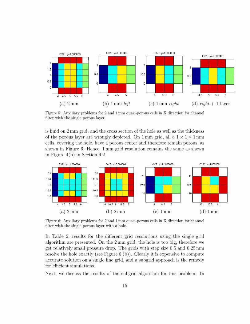
4.3. Channel filter with single porous layer with a hole

As a next example, the same filter geometry is considered as in subsection4.2 but with Uin = 2.8e − 03 and with a small hole in the porous layer -(x, y, z) : 4.5 ≤ x ≤ 5.5, 10.5 ≤ y ≤ 11.5, 10.5 ≤ z ≤ 11.5 mm. This holeis correctly resolved on 0.5 mm grid. On 2 mm grid, this 1× 1× 1 mm hole isexactly in the center of 2×2×2 mm coarse cell, as illustrated in Figure 6 (a)and (b). Figure 6 (a) is a view along the channel, whereas Figure 6 (b) is aview across the channel. Therefore, as opposed to the previous case, this cell

14

(a) 2 mm (b) 1 mm left (c) 1 mm right (d) right + 1 layer

Figure 5: Auxiliary problems for 2 and 1 mm quasi-porous cells in X direction for channelfilter with the single porous layer.

is fluid on 2 mm grid, and the cross section of the hole as well as the thicknessof the porous layer are wrongly depicted. On 1 mm grid, all 8 1× 1× 1 mmcells, covering the hole, have a porous center and therefore remain porous, asshown in Figure 6. Hence, 1 mm grid resolution remains the same as shownin Figure 4(b) in Section 4.2.

(a) 2 mm (b) 2 mm (c) 1 mm (d) 1 mm

Figure 6: Auxiliary problems for 2 and 1 mm quasi-porous cells in X direction for channelfilter with the single porous layer with a hole.

In Table 2, results for the different grid resolutions using the single gridalgorithm are presented. On the 2 mm grid, the hole is too big, therefore weget relatively small pressure drop. The grids with step size 0.5 and 0.25 mmresolve the hole exactly (see Figure 6 (b)). Clearly it is expensive to computeaccurate solution on a single fine grid, and a subgrid approach is the remedyfor efficient simulations.

Next, we discuss the results of the subgrid algorithm for this problem. In

15

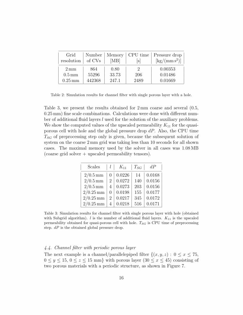
Grid Number Memory CPU time Pressure dropresolution of CVs [MB] [s] [kg/(mm s2)]

2 mm 864 0.80 2 0.003530.5 mm 55296 33.73 206 0.014860.25 mm 442368 247.1 2489 0.01669

Table 2: Simulation results for channel filter with single porous layer with a hole.

Table 3, we present the results obtained for 2 mm coarse and several (0.5,0.25 mm) fine scale combinations. Calculations were done with different num-ber of additional fluid layers l used for the solution of the auxiliary problems.We show the computed values of the upscaled permeability K11 for the quasi-porous cell with hole and the global pressure drop dP . Also, the CPU timeTSG of preprocessing step only is given, because the subsequent solution ofsystem on the coarse 2 mm grid was taking less than 10 seconds for all showncases. The maximal memory used by the solver in all cases was 1.08 MB(coarse grid solver + upscaled permeability tensors).

Scales l K11 TSG dP

2/0.5 mm 0 0.0226 14 0.01682/0.5 mm 2 0.0272 140 0.01562/0.5 mm 4 0.0273 203 0.01562/0.25 mm 0 0.0198 155 0.01772/0.25 mm 2 0.0217 345 0.01722/0.25 mm 4 0.0218 516 0.0171

Table 3: Simulation results for channel filter with single porous layer with hole (obtainedwith Subgrid algorithm). l is the number of additional fluid layers. K11 is the upscaledpermeability obtained for quasi-porous cell with hole. TSG is CPU time of preprocessingstep. dP is the obtained global pressure drop.

4.4. Channel filter with periodic porous layer

The next example is a channel/parallelepiped filter (x, y, z) : 0 ≤ x ≤ 75,0 ≤ y ≤ 15, 0 ≤ z ≤ 15 mm with porous layer (30 ≤ x ≤ 45) consisting oftwo porous materials with a periodic structure, as shown in Figure 7.

16

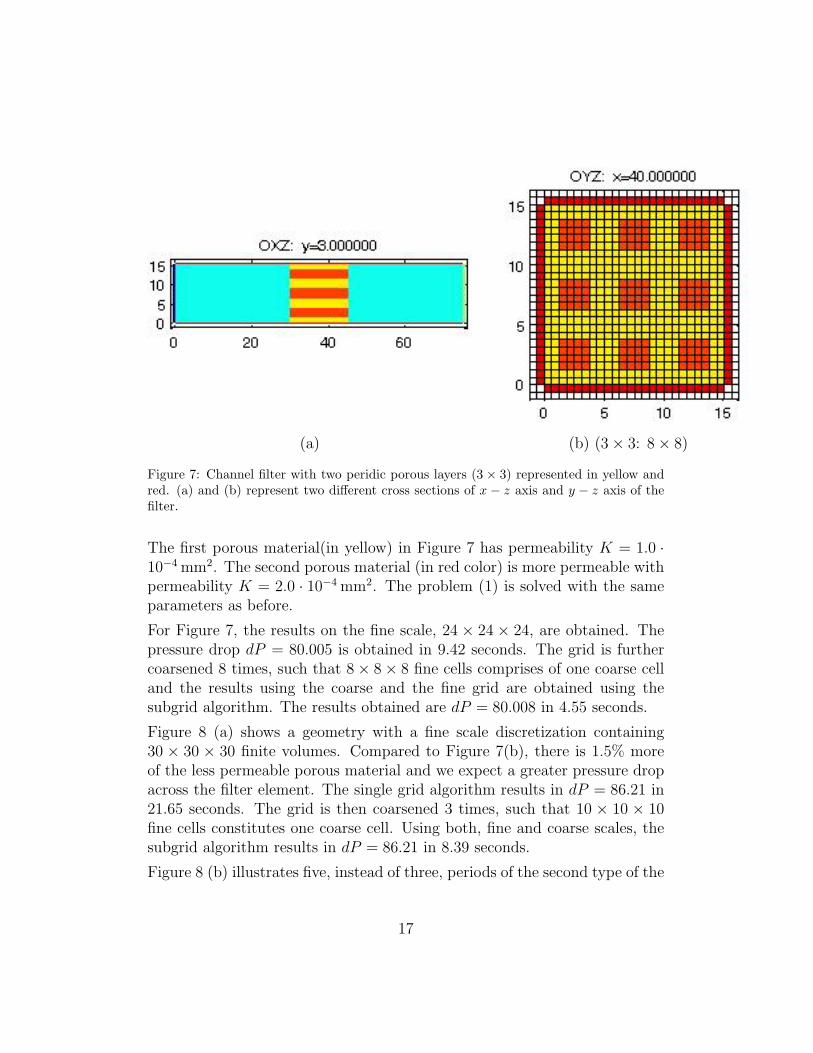
(a) (b) (3× 3: 8× 8)

Figure 7: Channel filter with two peridic porous layers (3 × 3) represented in yellow andred. (a) and (b) represent two different cross sections of x − z axis and y − z axis of thefilter.

The first porous material(in yellow) in Figure 7 has permeability K = 1.0 ·10−4 mm2. The second porous material (in red color) is more permeable withpermeability K = 2.0 · 10−4 mm2. The problem (1) is solved with the sameparameters as before.

For Figure 7, the results on the fine scale, 24 × 24 × 24, are obtained. Thepressure drop dP = 80.005 is obtained in 9.42 seconds. The grid is furthercoarsened 8 times, such that 8× 8× 8 fine cells comprises of one coarse celland the results using the coarse and the fine grid are obtained using thesubgrid algorithm. The results obtained are dP = 80.008 in 4.55 seconds.

Figure 8 (a) shows a geometry with a fine scale discretization containing30 × 30 × 30 finite volumes. Compared to Figure 7(b), there is 1.5% moreof the less permeable porous material and we expect a greater pressure dropacross the filter element. The single grid algorithm results in dP = 86.21 in21.65 seconds. The grid is then coarsened 3 times, such that 10 × 10 × 10fine cells constitutes one coarse cell. Using both, fine and coarse scales, thesubgrid algorithm results in dP = 86.21 in 8.39 seconds.

Figure 8 (b) illustrates five, instead of three, periods of the second type of the

17

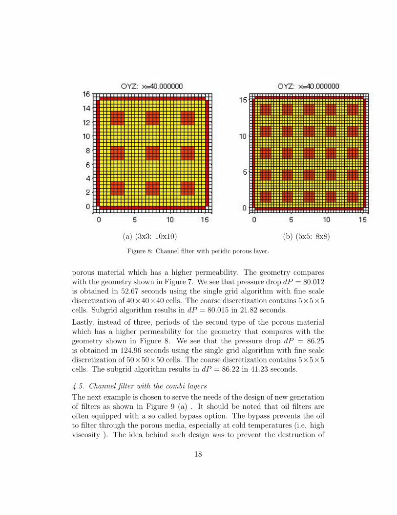
(a) (3x3: 10x10) (b) (5x5: 8x8)

Figure 8: Channel filter with peridic porous layer.

porous material which has a higher permeability. The geometry compareswith the geometry shown in Figure 7. We see that pressure drop dP = 80.012is obtained in 52.67 seconds using the single grid algorithm with fine scalediscretization of 40×40×40 cells. The coarse discretization contains 5×5×5cells. Subgrid algorithm results in dP = 80.015 in 21.82 seconds.

Lastly, instead of three, periods of the second type of the porous materialwhich has a higher permeability for the geometry that compares with thegeometry shown in Figure 8. We see that the pressure drop dP = 86.25is obtained in 124.96 seconds using the single grid algorithm with fine scalediscretization of 50×50×50 cells. The coarse discretization contains 5×5×5cells. The subgrid algorithm results in dP = 86.22 in 41.23 seconds.

4.5. Channel filter with the combi layers

The next example is chosen to serve the needs of the design of new generationof filters as shown in Figure 9 (a) . It should be noted that oil filters areoften equipped with a so called bypass option. The bypass prevents the oilto filter through the porous media, especially at cold temperatures (i.e. highviscosity ). The idea behind such design was to prevent the destruction of

18

the filter due to the high pressure in such cases. Instead, the oil bypassesthe filtering medium via some small pipe. Obviously, the bypassed oil is notfiltered in this situation. Alternatively, the new league of filters are designedwithout the bypass option, but with an additional layer of a fine perforatedfilter layer that allows the oil to flow through the holes at cold temperatures.Additionally, a coarse filter layer in the form of a solid mesh is added to filterout the large particles. With the support of the numerical simulations, thesize of the holes and the distance between the two porous layers are designedsuch that most oil flows through the porous part of the first layer at hightemperature, and not through the holes. It is common understanding thatthe porous layers are the primary cause of the pressure drop across the filter.This is true only when the filter element is designed in a way that there isenough space between the inlet(bottom) and the porous layer, and betweenthe porous layer and the outlet(top). Therefore, we study this filter in asimplified geometry, i.e. a simple channel geometry as shown in Figure 9(b). The considered filter element is parallel piped (x, y, z) : 2 ≤ x ≤ 67,−11 ≤ y ≤ −2, −67 ≤ z ≤ −2 mm with two filtering porous layers and asupporting solid mesh between them, as shown in Figure 10 (b). Additionally,the first porous layer (−8 ≤ y ≤ −7) has a set of 6 × 6 holes, as shown inFigure 10 (b), where each hole is a cube: 1 × 1 × 1 mm, as illustrated inFigure 11 (a).When using the 2 mm resolution, the mesh layer is not captured at all andboth porous layers have the wrong, doubled thickness, on this grid: −8 ≤y ≤ −6 and −6 ≤ y ≤ −4, respectively. The 1 mm grid represents thechannel and all three layers (including the solid mesh) correctly except forthe holes in the first porous layer. As shown in Figure 11, all 4 1× 1× 1 mmcells, covering the hole, have a porous center and therefore are represented asporous in 1 mm grid. The 0.5 and 0.25 mm grids resolve the whole geometryof the filter exactly.

System 1 is solved with the following flow parameters: Uin = 3.944773 mm/s,ρ = 1.0 · 10−7 kg/mm3, µ = 1.0 · 10−4 kg/(mm s), isotropic permeability offirst porous layer, K = 4.2 · 10−5 mm2, and isotropic permeability of secondporous layer, K = 7.5 · 10−4 mm2. Note that in this test case the main flowis in Y direction.

In Table 4, the results of single grid algorithm for different grid resolutions arepresented. It is due to the aforementioned errors in the geometry resolutionfor 2 to 1 mm grids, that the resulting pressure drop is over estimated. As one

19

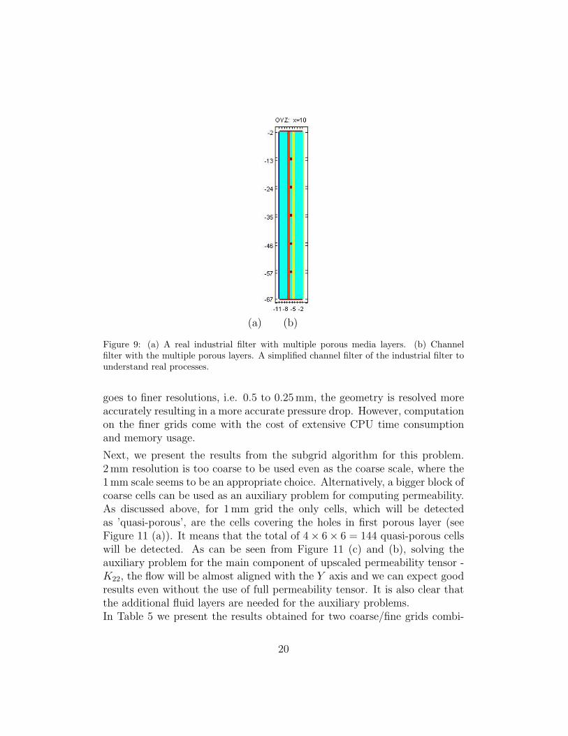
(a) (b)

Figure 9: (a) A real industrial filter with multiple porous media layers. (b) Channelfilter with the multiple porous layers. A simplified channel filter of the industrial filter tounderstand real processes.

goes to finer resolutions, i.e. 0.5 to 0.25 mm, the geometry is resolved moreaccurately resulting in a more accurate pressure drop. However, computationon the finer grids come with the cost of extensive CPU time consumptionand memory usage.

Next, we present the results from the subgrid algorithm for this problem.2 mm resolution is too coarse to be used even as the coarse scale, where the1 mm scale seems to be an appropriate choice. Alternatively, a bigger block ofcoarse cells can be used as an auxiliary problem for computing permeability.As discussed above, for 1 mm grid the only cells, which will be detectedas ’quasi-porous’, are the cells covering the holes in first porous layer (seeFigure 11 (a)). It means that the total of 4× 6× 6 = 144 quasi-porous cellswill be detected. As can be seen from Figure 11 (c) and (b), solving theauxiliary problem for the main component of upscaled permeability tensor -K22, the flow will be almost aligned with the Y axis and we can expect goodresults even without the use of full permeability tensor. It is also clear thatthe additional fluid layers are needed for the auxiliary problems.In Table 5 we present the results obtained for two coarse/fine grids combi-

20

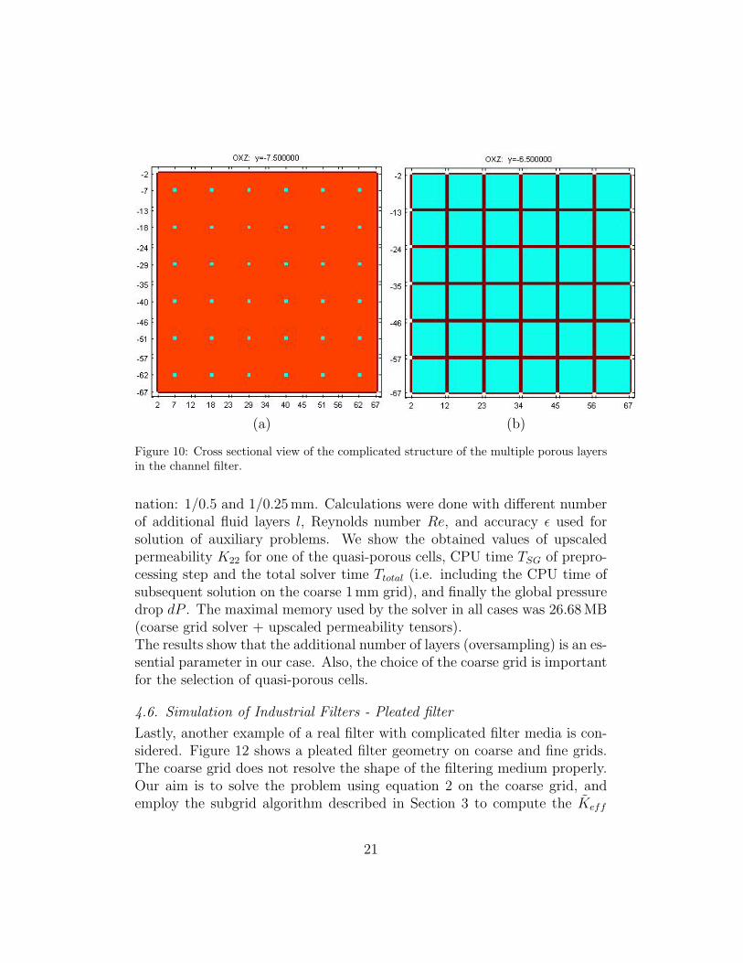
(a) (b)

Figure 10: Cross sectional view of the complicated structure of the multiple porous layersin the channel filter.

nation: 1/0.5 and 1/0.25 mm. Calculations were done with different numberof additional fluid layers l, Reynolds number Re, and accuracy ε used forsolution of auxiliary problems. We show the obtained values of upscaledpermeability K22 for one of the quasi-porous cells, CPU time TSG of prepro-cessing step and the total solver time Ttotal (i.e. including the CPU time ofsubsequent solution on the coarse 1 mm grid), and finally the global pressuredrop dP . The maximal memory used by the solver in all cases was 26.68 MB(coarse grid solver + upscaled permeability tensors).The results show that the additional number of layers (oversampling) is an es-sential parameter in our case. Also, the choice of the coarse grid is importantfor the selection of quasi-porous cells.

4.6. Simulation of Industrial Filters - Pleated filter

Lastly, another example of a real filter with complicated filter media is con-sidered. Figure 12 shows a pleated filter geometry on coarse and fine grids.The coarse grid does not resolve the shape of the filtering medium properly.Our aim is to solve the problem using equation 2 on the coarse grid, andemploy the subgrid algorithm described in Section 3 to compute the Keff

21

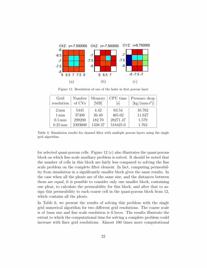
(a) (b) (c)

Figure 11: Resolution of one of the holes in first porous layer

Grid Number Memory CPU time Pressure dropresolution of CVs [MB] [s] [kg/(mm s2)]

2 mm 5445 4.42 63.54 16.7621 mm 37400 26.49 465.02 11.627

0.5 mm 299200 182.70 28271.47 1.5790.25 mm 2393600 1338.37 518425.0 1.762

Table 4: Simulation results for channel filter with multiple porous layers using the singlegrid algorithm.

for selected quasi-porous cells. Figure 12 (c) also illustrates the quasi-porousblock on which fine scale auxiliary problem is solved. It should be noted thatthe number of cells in this block are fairly less compared to solving the finescale problem on the complete filter element. In fact, computing permeabil-ity from simulation in a significantly smaller block gives the same results. Inthe case when all the pleats are of the same size, and the distances betweenthem are equal, it is possible to consider only one smaller block, containingone pleat, to calculate the permeability for this block, and after that to as-sign this permeability to each coarse cell in the quasi-porous block from 12,which contains all the pleats.

In Table 6, we present the results of solving this problem with the singlegrid numerical algorithm for two different grid resolutions. The coarse scaleis of 1mm size and fine scale resolution is 0.5mm. The results illustrate theextent to which the computational time for solving a complete problem couldincrease with finer grid resolutions. Almost 100 times more computational

22

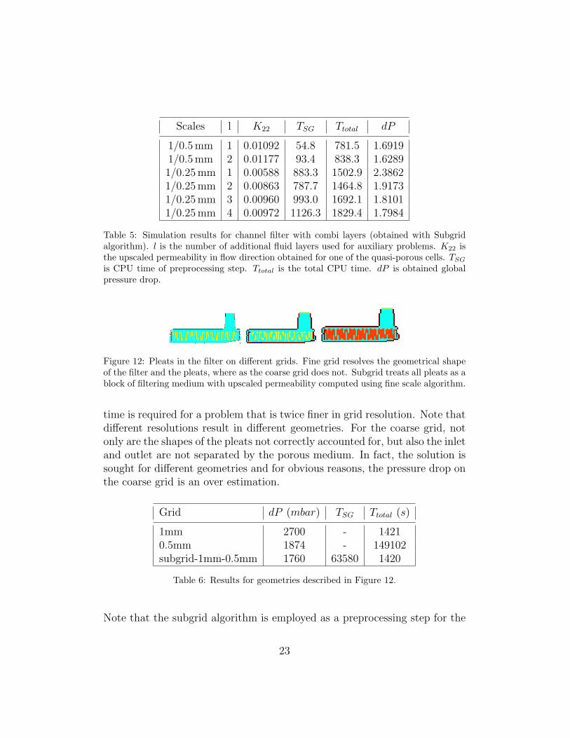
Scales l K22 TSG Ttotal dP

1/0.5 mm 1 0.01092 54.8 781.5 1.69191/0.5 mm 2 0.01177 93.4 838.3 1.62891/0.25 mm 1 0.00588 883.3 1502.9 2.38621/0.25 mm 2 0.00863 787.7 1464.8 1.91731/0.25 mm 3 0.00960 993.0 1692.1 1.81011/0.25 mm 4 0.00972 1126.3 1829.4 1.7984

Table 5: Simulation results for channel filter with combi layers (obtained with Subgridalgorithm). l is the number of additional fluid layers used for auxiliary problems. K22 isthe upscaled permeability in flow direction obtained for one of the quasi-porous cells. TSG

is CPU time of preprocessing step. Ttotal is the total CPU time. dP is obtained globalpressure drop.

Figure 12: Pleats in the filter on different grids. Fine grid resolves the geometrical shapeof the filter and the pleats, where as the coarse grid does not. Subgrid treats all pleats as ablock of filtering medium with upscaled permeability computed using fine scale algorithm.

time is required for a problem that is twice finer in grid resolution. Note thatdifferent resolutions result in different geometries. For the coarse grid, notonly are the shapes of the pleats not correctly accounted for, but also the inletand outlet are not separated by the porous medium. In fact, the solution issought for different geometries and for obvious reasons, the pressure drop onthe coarse grid is an over estimation.

Grid dP (mbar) TSG Ttotal (s)

1mm 2700 - 14210.5mm 1874 - 149102subgrid-1mm-0.5mm 1760 63580 1420

Table 6: Results for geometries described in Figure 12.

Note that the subgrid algorithm is employed as a preprocessing step for the

23

single grid algorithm. Moreover, in industry, the subgrid method benefitsfrom the fact that for each fixed geometry, many simulations are done usingdifferent physical parameters, such as density, viscosity, inflow velocities etc.for assessing the filter performance. In this case, the subgrid method can beused only once and precomputed upscaled permeabilities for the quasi-porouscells/blocks can be further used in subsequent simulations.

5. Summary

A subgrid method is considered as a computational method for achievingdesired accurate solutions for our problem. It is mainly employed for caseswhere the coarse computational grid is unable to accurately account for thecomplicated geometry and/or the filter media. The single grid algorithmis used as the building block for solving auxiliary problems on the quasi-porous cells and for solving the global coarse scale problem, with specialemphasis based on re-usability of solvers. The method emphasizes on thedetermination of upscaled quantities for use in subsequent coarse scale globalsimulations. Fine scale solution is sought only on some quasi-porous cell/sor collectively on a block (a collection of coarse cells). The results werepresented for the computer simulation experiments using three dimensionalmodels of oil filters. It is observed that the cell/block permeability is stronglyinfluenced by the resolving grid. The CPU time and memory usage is reducedsignificantly using the subgrid method with the resulting desired accuracy ofthe pressure drop, which characterizes the flow through filters.

[1] A. Kumar, Numerical Estimation of Surface Parameters by Level SetMethods, PhD Thesis, Technical University of Kaiserslautern, 2003.

[2] A. J. Chorin, Numerical Solution of Navier-Stokes equation, Mathemat-ics of Computation 22 (1968), 745-760.

[3] A. F. Gulbransen, V.L. Hauge, K.A. Lie, A Multiscale Mixed Finite Ele-ment Method for Vuggy and Naturally Fractured Reservoirs, 21st NordicSeminar on Computational Mechanics, Trondheim, 149-152, 2008.

[4] C.A.J. Fletcher, Computational techniques for fluid dynamics. Springer,Berlin etc., 1991.

24

[5] G. Bonfigli, P. Jenny, An efficient multi-scale poisson solver for theincompressible navier-stokes equations with immersed boundaries. J.Comp. Phys., 228(12), 2009.

[6] G. Allaire, Homogenization of the Navier-Stokes equations in open setsperforated with tiny holes. i: Abstract framework, a volume distributionof holes, Arch. Ration. Mech. Anal. 113 (1991), no. 3, 209-259.

[7] H.C. Brinkman, A calculation of the viscous force exerted by a flowingfluid on a dense swarm of particles, Appli. Sci. Res., t. A1, (1947), 27-34.

[8] H. Hajibeygi, G. Bonfigli, M. A. Hesse, and P. Jenny. Iterative multiscalefinite-volume method. J. Comp. Phys., 227(19):8604-8621, Oct 2008.

[9] J. Willems, Numerical Upscaling for Multiscale Flow Problems, PhDthesis, Technical University of Kaiserslautern, 2009.

[10] K. R. Rajagopal, On a hierarchy of approximate models for flows ofincompressible fluids through porous solids, Math. Models Meth. Appl.Sci., 17 (2007), 215-252.

[11] L.J. Durlofsky, Numerical calculation og equivalent grid block perme-ability tensors for heterogeneous porous media, Water Resources Re-search 27, 669-708, 1991.

[12] M. Kaviany, Principles of Heat Transfer in Porous Media. Springer, NewYork etc., 1991.

[13] M. Dedering, W. Stausberg, O. Iliev, Z. Lakdawala, R. Ciegis, V.Starikovicius, On new Challenges for CFD Simulation in Filtration, Pro-ceedings of World Filtration Congress, Leipzig, 2008.

[14] O. Iliev, Z. Lakdawala, R. Ciegis, V. Starikovicius, M. Dedering,P.Popov, Advanced CFD simulation of filtration processes, Proceedingsof Filtech, Wiesbaden, 2009.

[15] O. Iliev, V. Laptev, On numerical simulation of flow through oil filters.Comput. Vis. Sci., 6 (2004) 139–146.

[16] O. Iliev, V. Laptev, D. Vassileva, Algorithms and software for computersimulation of flow through oil filters. Proc. FILTECH Europa, 2003,Dusseldorf, pp.327–334.

25

[17] O. Iliev, R.D. Lazarov, and J. Willems, Fast numerical upscaling ofheat equation for fibrous materials, J. Computing and Visualization inScience, 2009.

[18] Ph. Angot, Analysis of singular perturbations on the Brinkman problemfor fictitious domain models of viscous flows. Math. Meth. Appl. Sci.,22 (1999) 1395–1412.

[19] P. Gresho, R. Sani, Incompressible flow and the finite element method.Volume 1: Advection-diffusion and isothermal laminar flow. In collabo-ration with M. S. Engelman. Chichester: Wiley. 1044 p. (1998).

[36] M. Griebel and M. Klitz. Homogenisation and Numerical Simulationof Flow in Geometries with Textile Microstructures. SIAM MMS, 2009.Submitted. Also available as SFB611 preprint no 404 / 2008.

[21] P. Jenny and I. Lunati. Multi-scale finite-volume method for ellipticproblems with heterogeneous coefficients and source terms. Proc. Appl.Math. Mech., 6(1):485-486, 2006.

[22] R. Ciegis, O. Iliev, Z. Lakdawala, On parallel numerical algorithms forsimulating industrial filtration problems. Computational Methods in Ap-plied Mathematics 7(2), 118-134(2007).

[23] T.Y. Hou, Y. Efendiev, Multiscale Finite Element Methods. Surveysand Tutorials in the Applied Mathematical Sciences, Band 4, Springer,2009.

[24] T. Arbogast, Analysis of a two-scale, locally conservative subgrid up-scaling for elliptic problems, SIAM J. Numer. Anal. 42 (2004), no. 2,576598.

[25] T. Arbogast, S. L. Bryant, A two-scale numerical subgrid technique forwaterflood simulations, SPE Journal 7 (2002) 446-457.

[26] T. Arbogast, Implementation of a locally conservative numerical subgridupscaling scheme for two-phase Darcy flow, Computational Geosciences6, 453-481, 2002.

[27] U. Hornung. Homogenization and porous media, Springer Verlag NewYork Inc., New York, USA, 1996.

26

[28] V. Starikovicius, R. Ciegis, O. Iliev, Z.Lakdawala, A parallel solver forthe 3D Simulation of Flows through Oil Filters, Springer Optimizationand its applications, Volume 27, 181-191(2008).

[29] V.V. Jikov, S.M. Kozlov, Oleinik O.A., Homogenization of DifferentialOperators and Integral Functionals, Springer-Verlag, Berlin, 1994.

[30] V. Laptev, Numerical solution of coupled flow in plain and porous media.PhD thesis, Technical University of Kaiserslautern, 2003.

[31] X.H. Wu, Y. Efendiev and T.Y. Hou, Analysis of upscaling absolutepermeability. Discrete Contin. Dyn. Syst., Series B 2, No. 2, 185-204(2002).

[32] Y. Chen, L.J. Durlofsky, M. Gerritsen, X.H. Wen, A Coupled Local-Global Upscaling Approach for Simulating Flow in Highly Heteroge-neous Formations, Advances in Water Resources, 26, 1041-1060 2003.

[33] Y. Jung, S. Torquato, Fluid permeabilities of triply periodic minimalsurfaces, Physical Review Em 72, 056319, 2005.

[34] A. Sangani, A.Acrivos, Int. J. Multiphase Flow, 8, 343, 1982.

[35] James H. Bramble and Joseph E. Pasciak, 1988. A preconditioning tech-nique for indefinite systems resulting from mixed approximations of el-liptic problems. Math. Comp., 50(181): 1-17.

[36] M. Griebel, M. Klitz. Homogenisation and Numerical Simulation of Flowin Geometries with Textile Microstructures. SIAM MMS, 2009.

27