ollivier’s ricci curvature, local clustering and curvature ...ollivier’s ricci curvature, local...

Discrete Comput Geom (2014) 51:300–322DOI 10.1007/s00454-013-9558-1

Ollivier’s Ricci Curvature, Local Clusteringand Curvature-Dimension Inequalities on Graphs

Jürgen Jost · Shiping Liu

Received: 23 May 2012 / Accepted: 21 October 2013 / Published online: 13 November 2013© Springer Science+Business Media New York 2013

Abstract In this paper, we explore the relationship between one of the most ele-mentary and important properties of graphs, the presence and relative frequency oftriangles, and a combinatorial notion of Ricci curvature. We employ a definition ofgeneralized Ricci curvature proposed by Ollivier in a general framework of Markovprocesses and metric spaces and applied in graph theory by Lin–Yau. In analogy withcurvature notions in Riemannian geometry, we interpret this Ricci curvature as a con-trol on the amount of overlap between neighborhoods of two neighboring vertices. Itis therefore naturally related to the presence of triangles containing those vertices, ormore precisely, the local clustering coefficient, that is, the relative proportion of con-nected neighbors among all the neighbors of a vertex. This suggests to derive lowerRicci curvature bounds on graphs in terms of such local clustering coefficients. Wealso study curvature-dimension inequalities on graphs, building upon previous workof several authors.

J. Jost · S. Liu (B)Max Planck Institute for Mathematics in the Sciences, Leipzig 04103, Germanye-mail: [email protected]

J. Joste-mail: [email protected]

J. JostDepartment of Mathematics and Computer Sciences, University of Leipzig, Leipzig 04103, Germany

J. JostSanta Fe Institute for the Sciences of Complexity, Santa Fe, NM 87501, USA

S. LiuAcademy of Mathematics and Systems Science, Chinese Academy of Sciences, Beijing 100190,China

Present address:S. LiuDepartment of Mathematical Sciences, Durham University, Durham DH1 3LE, UKe-mail: [email protected]

mailto:[email protected]



Discrete Comput Geom (2014) 51:300–322 301

Keywords Ollivier’s Ricci curvature · Curvature dimension inequality · Localclustering · Graph Laplace operator

1 Introduction

When one studies empirical graphs, one of the most obvious and basic propertiesto investigate is the presence and number of triangles, that is, connected triples ofvertices. In bipartite graphs, for instance, there are no triangles, whereas in a com-plete graph, every triple of vertices constitutes a triangle. A basic observation then isthat when two neighboring vertices are contained in a triangle, their neighborhoodsof radius 1 (let us assign to every edge the length 1 for the discussion in this intro-duction) share the third vertex of the triangle. That is, the more triangles those twoneighboring vertices are contained in, the larger the overlap of their neighborhoods.This suggests an analogy with the notion of Ricci curvature in Riemannian geometrywhere a lower bound on the Ricci curvature also controls the amount of overlapsof distance balls from below. This is what we are going to explore in a quantitativemanner in this paper.

In fact, Ricci curvature is a fundamental concept in Riemannian geometry, see e.g.[18]. It is a quantity computed from second derivatives of the metric tensor. It controlshow fast geodesics starting at the same point diverge on average. Equivalently, itcontrols how fast the volume of distance balls grows as a function of the radius.As already indicated, it also controls the amount of overlap of two distance balls interms of their radii and the distance between their centers. In fact, such lower boundsfollow from a lower bound on the Ricci curvature. It was then natural to look forgeneralizations of such phenomena on metric spaces more general than Riemannianmanifolds. That is, the question to find substitutes for the lower bounds on the abovementioned second derivative combinations of the metric tensor that yield the samegeometric control on a general metric space. By now, there exist several insightfuldefinitions of synthetic Ricci curvature on general metric measure spaces, see Sturm[29, 30], Lott–Villani [22], Ohta [23], Ollivier [24] etc.

As indicated, in this paper, we want to explore the implications of such ideasin graph theory. The geometric idea is that a lower Ricci curvature bound preventsgeodesics from diverging too fast and balls from growing too fast in volume. On agraph, the analogue of geodesics starting in different directions, but eventually ap-proaching each other again, would be a triangle. Therefore, it is natural that the Riccicurvature on a graph should be related to the relative abundance of triangles. The lat-ter is captured by the local clustering coefficient introduced by Watts–Strogatz [33].Thus, the intuition of Ricci curvature on a graph should play with the relative fre-quency of triangles a vertex shares with its neighbors. In fact, more precisely, sincethe local clustering coefficient averages over the neighbors of a vertex, this shouldreally related to some notion of scalar curvature, as an average of Ricci curvatures indifferent directions, that is, for different neighbors of a given vertex.

Among the several definitions of generalized Ricci curvature in the literature men-tioned above, the one of Ollivier works particularly well on discrete spaces likegraphs. It is formulated in terms of the transportation distance between local mea-sures:

κ(x, y) := 1 − W1(mx,my), (1.1)

302 Discrete Comput Geom (2014) 51:300–322

where x, y are vertices in our graph that are neighbors (written as x ∼ y) and themeasure mx = 1

dx, where dx is the degree of x, puts equal weight on all neighbors.

W1(mx,my) is the transportation distance between the two measures mx and my (de-fined more precisely below). When two balls strongly overlap, as is the case in Rie-mannian geometry when the Ricci curvature has a large lower bound, then it is easierto transport the mass of one to the other. Analogously, in the graph case, when the twovertices share many triangles, then the transportation distance should be smaller, andthe curvature therefore correspondingly larger. This is the idea of Ollivier’s definitionas we see it and explore in this paper. We shall obtain both upper and lower boundsfor Ollivier’s Ricci curvature on graphs in Sect. 3, which are optimal on many graphs.

Let us now formulate our main result (recalled and proved below as Theorem 3).

Theorem 1 On a locally finite graph, we put for any pair of neighboring verticesx, y,

�(x, y) := number of triangles which include x, y as vertices =∑

x1,x1∼x,x1∼y

1.

We then have

κ(x, y) ≥ −(

1 − 1

dx

− 1

dy

− �(x, y)

dx ∧ dy

)

+−

(1 − 1

dx

− 1

dy

− �(x, y)

dx ∨ dy

)

+

+ �(x, y)

dx ∨ dy

. (1.2)

where s+ := max(s,0), s ∨ t := max(s, t), s ∧ t := min(s, t).

This equality is sharp for instance for a complete graph of n vertices where the leftand the right hand side both equal to n−2

n−1 .The local clustering coefficient introduced by Watts–Strogatz [33] is

c(x) := number of edges between neighbors of x

number of possible existing edges between neighbors of x, (1.3)

which measures the extent to which neighbors of x are directly connected, i.e.,

c(x) = 1

dx(dx − 1)

∑

y,y∼x

�(x, y). (1.4)

Thus, this local clustering coefficient is an average over the �(x, y) for the neighborsof x. Thus, we might also introduce some kind of scalar curvature (suggested inProblem Q in Ollivier [25]) as

κ(x) := 1

dx

∑

y,y∼x

κ(x, y). (1.5)

For illustration, let us consider the case where our graph is d-regular, that is, dz = d

for all vertices z. When 1 ≥ 2d

+ �(x,y)d

for all y ∼ x, we would then get

κ(x) ≥ −2 + 4

d+ 3(d − 1)

dc(x). (1.6)


This example nicely illustrates the relation between Ollivier’s curvature and theWatts–Strogatz clustering coefficient.

Without the triangle terms �(x, y) (which is the crucial term for our purposes),Theorem 1 is due to Lin–Yau [19, 21], and we take their proof as our starting point.Lin–Yau also obtain analogues of Bochner type inequalities and eigenvalue estimatesas known from Riemannian geometry.

In Riemannian geometry, the Bochner formula encodes deep analytic propertiesof Ricci curvature. It is a key ingredient in proving many results, e.g. the spectralgap of the Laplace–Beltrami operator. A lower bound of the Ricci curvature impliesa curvature-dimension inequality involving the Laplace–Beltrami operator throughthe Bochner formula. In an important work, Bakry and Émery [2, 3] generalize thisinequality to generators of Markov semigroups, which works on measure spaces.Their inequality contains plentiful information and implies a lot of functional in-equalities including spectral gap inequalities, Sobolev inequalities, and logarithmicSobolev inequalities and many celebrated geometric theorems (see [1] and the refer-ences therein). Lin–Yau [21] study such inequalities on locally finite graphs.

In the present paper, we also want to find relations on locally finite graphs be-tween Ollivier’s Ricci curvature and Bakry–Émery’s curvature-dimension inequal-ities, which represent the geometric and analytic aspects of graphs, respectively.Again, this is inspired by Riemannian geometry where one may attach a Brownianmotion with a drift to a Riemannian metric [24]. We also mention that the definitionsgiven by Sturm and Lott–Villani are also consistent with that of Bakry–Émery [22,29, 30]. So exploring the relations on nonsmooth spaces may provide a good point ofview to connect Ollivier’s definition to Sturm and Lott–Villani’s (in this respect, seealso Ollivier–Villani [26]). In Sect. 4, we use the local clustering coefficient again toestablish more precise curvature-dimension inequalities than those of Lin–Yau [21].And with this in hand, we prove curvature-dimension inequalities under the conditionthat Ollivier’s Ricci curvature of the graph is positive.

Further analytical results following from curvature-dimension inequalities on fi-nite graphs have been described in [19], and Lin–Lu–Yau [20] study a modified def-inition of Ollivier’s Ricci curvature on graphs. Recently, Paeng [27] studied upperbounds for the diameter and volume of finite simple graphs in terms of Ollivier’sRicci curvature. For other works of synthetic Ricci curvatures on discrete spaces, seeDodziuk–Karp [14], Chung–Yau [9], Bonciocat–Sturm [7], and on cell complexessee Forman [17], Stone [28] etc.

We point out that, as in Riemannian geometry, both Ollivier’s Ricci curvature andBakry–Émery’s curvature-dimension inequality can give lower bound estimates ofthe first eigenvalue λ1 for the Laplace operator (see Ollivier [24], Bakry [1]). There-fore our results in fact relate λ1 to the Watts–Strogatz local clustering coefficient,or the number of cycles with length 3. In [10], Diaconis and Stroock obtain severalgeometric bounds for eigenvalues of graphs, one of which is related to the numberof odd length cycles. For more geometric quantities and methods concerning eigen-value estimates in the study of Markov chains, see [11–13] and the references therein.We further explore the interaction between Ollivier’s Ricci curvature and eigenvaluesestimates in joint work with Frank Bauer, see [6].

In this paper, G = (V ,E) will denote an undirected connected simple graph with-out loops, where V is the set of vertices and E is the set of edges. V could be an


infinite set. But we require that G is locally finite, i.e., for every x ∈ V , the numberof edges connected to x is finite. For simplicity and in order to see more geometry,we mainly work on unweighted graphs. But we will also derive similar results onweighted graphs. In that case, we denote by wxy the weight associated to x, y ∈ V ,where x ∼ y (we may simply put wxy = 0 if x and y are not neighbors, to simplifythe notation). The unweighted case corresponds to wxy = 1 whenever x ∼ y. Thedegree of x ∈ V is dx = ∑

y,y∼x wxy .

2 Ollivier’s Ricci Curvature and Bakry–Émery’s Calculus

In this section, we present some basic facts about Ollivier’s Ricci curvature andBakry–Emery’s Γ2 calculus, in particular on graphs.

2.1 Ollivier’s Ricci Curvature

Ollivier’s Ricci curvature works on a general metric space (X,d), on which we at-tach to each point x ∈ X a probability measure mx(·). We denote this structure by(X,d,m).

For a locally finite graph G = (V ,E), we define the metric d as follows. Forneighbors x, y, d(x, y) = 1. For general distinct vertices x, y, d(x, y) is the length ofthe shortest path connecting x and y, i.e. the number of edges of the path. We attachto each vertices x ∈ V a probability measure

mx(y) ={

wxy

dx, if y ∼ x;

0, otherwise.(2.1)

An intuitive illustration of this is a random walker that sits at x and then choosesamongst the neighbors of x with equal probability 1

dx.

Definition 1 (Ollivier) On (X,d,m), for any two distinct points x, y ∈ X, the(Ollivier–) Ricci curvature of (X,d,m) along (xy) is defined as

κ(x, y) := 1 − W1(mx,my)

d(x, y). (2.2)

Here, W1(mx,my) is the optimal transportation distance between the two proba-bility measures mx and my , defined as follows (cf. Villani [31, 32], Evans [16]).

Definition 2 For two probability measures μ1, μ2 on a metric space (X,d), the trans-portation distance between them is defined as

W1(μ1,μ2) := infξ∈∏

(μ1,μ2)

∫

X×X

d(x, y) dξ(x, y), (2.3)

where∏

(μ1,μ2) is the set of probability measures on X × X projecting to μ1and μ2.


In other words, ξ satisfies

ξ(A × X) = μ1(A), ξ(X × B) = μ2(B), ∀A,B ⊂ X.

Remark 1 Intuitively, this distance measures the optimal cost to move one pileof sand to another one with the same mass. For case of a graph G = (G,d,m),the supports of mx and my are finite discrete sets, and thus, ξ is just a ma-trix with terms ξ(x′, y′) representing the mass moving from x′ ∈ support of mx toy′ ∈ support of my . That is, in this case,

W1(mx,my) = infξ

∑

x′,x′∼x

∑

y′,y′∼y

d(x′, y′)ξ

(x′, y′),

where the infimum is taken over all matrices ξ which satisfy

∑

x′,x′∼x

ξ(x′, y′) = wyy′

dy

,∑

y′,y′∼y

ξ(x′, y′) = wxx′

dx

.

We also call ξ a transfer plan. If we can find a particular transfer plan, we then get anupper bound for W1 and therefore a lower bound for κ .

A very important property of transportation distance is the Kantorovich duality(see, e.g. Theorem 1.14 in Villani [31]). We state it here in our particular graph set-ting.

Proposition 1 (Kantorovich Duality)

W1(mx,my) = supf,1−Lip

[ ∑

z,z∼x

f (z)mx(z) −∑

z,z∼y

f (z)dmy(z)

],

where the supremum is taken over all functions on G that satisfy∣∣f (x) − f (y)

∣∣ ≤ d(x, y),

for any x, y ∈ V , x �= y.

From this property, a good choice of a 1-Lipschitz function f will yield a lowerbound for W1 and therefore an upper bound for κ .

Remark 2 We list some basic first observations about this curvature concept (seeOllivier [24]):

• κ(x, y) ≤ 1.• Rewriting (2.2) gives W1(mx,my) = d(x, y)(1 − κ(x, y)), which is analogous to

the expansion in the Riemannian case.• A lower bound κ(x, y) ≥ k for any x, y ∈ X implies

W1(mx,my) ≤ (1 − k)d(x, y), (2.4)

which can be seen as some kind of Lipschitz continuity of measures.


2.2 Bakry–Émery’s Curvature-Dimension Inequality

2.2.1 Laplace Operator

We will study the following operator which is an analogue of the Laplace–Beltramioperator in Riemannian geometry.

Definition 3 The Laplace operator on (X,d,m) is defined as follows:

�f (x) =∫

X

f (y)dmx(y) − f (x), for functions f : X −→ R. (2.5)

For our choice of {mx(·)}, this is the graph Laplacian studied by many authors,see e.g. [4, 5, 8, 14, 21].

2.2.2 Bochner Formula and Curvature-Dimension Inequality

In the Riemannian case, many analytical consequences of a lower bound of the Riccicurvature are obtained through the well-known Bochner formula,

1

2�

(|∇f |2) = |Hessf |2 + ⟨∇(�f ),∇f⟩ + Ric(∇f,∇f ).

Analytically, |Hessf |2 is difficult to define on a nonsmooth space. But usingSchwarz’s inequality, we have

|Hessf |2 ≥ (�f )2

m,

where m is the dimension constant. So we can use

1

2�

(|∇f |2) ≥ (�f )2

m+ ⟨∇(�f ),∇f

⟩ + K|∇f |2 (2.6)

to characterize Ric ≥ K .Bakry–Émery [1–3] take this inequality as the starting point and directly use the

operators to define curvature bounds. Starting from an operator �, they define itera-tively,

Γ0(f, g) = fg,

Γ (f,g) = 1

2

{�Γ0(f, g) − Γ0(f,�g) − Γ0(�f,g)

},

Γ2(f, g) = 1

2

{�Γ (f,g) − Γ (f,�g) − Γ (�f,g)

}.

In fact, Γ (f,f ) is an analogue of |∇f |2, and Γ2(f,f ) is an analogue of 12�|∇f |2 −

〈∇(�f ),∇f 〉 in (2.6).


Definition 4 We say an operator � satisfies a curvature-dimension inequalityCD(m,K) if for all functions f in the domain of the operator

Γ2(f,f )(x) ≥ 1

m

(�f (x)

)2 + K(x)Γ (f,f )(x), ∀x ∈ X, (2.7)

where m ∈ [1,+∞] is the dimension parameter, K(x) is the curvature function.

As studied in Lin–Yau [21], applying this construction to the operator (2.5) gives

Γ (f,f )(x) = 1

2

∫

X

(f (y) − f (x)

)2dmx(y). (2.8)

In fact generally

Γ (f,g)(x) = 1

2

∫

X

(f (y) − f (x)

)(g(y) − g(x)

)dmx(y).

For the sake of convenience, we will denote

Hf(x) := 1

4

∫

X

∫

X

(f (x) − 2f (y) + f (z)

)2dmy(z) dmx(y).

By the calculation in Lin–Yau [21] we get

�Γ (f,f )(x) = 2 Hf(x)

−∫

X

∫

X

(f (x) − 2f (y) + f (z)

)(f (x) − f (y)

)dmy(z) dmx(y),

2Γ (f,�f )(x) = −(�f (x)

)2

−∫

X

∫

X

(f (z) − f (y)

)(f (x) − f (y)

)dmy(z) dmx(y),

and then,

Γ2(f,f ) = Hf(x) − Γ (f,f )(x) + 1

2

(�f (x)

)2. (2.9)

3 Ollivier’s Ricci Curvature and Triangles

In this section, we mainly prove lower bounds for Ollivier’s Ricci curvauture onlocally finite graphs. In particular we shall explore the implication between lowerbounds of the curvature and the number of triangles including neighboring vertices;the latter is encoded in the local clustering coefficient. We remark that we only needto bound κ(x, y) from below for neighboring x, y, since by the triangle inequalityof W1, this will also be a lower bound for κ(x, y) of any pair of x, y. (See Proposi-tion 19 in Ollivier [24].)


3.1 Unweighted Graphs

In this subsection, we only consider unweighted graphs.In Lin–Yau [21], they prove a lower bound of Ollivier’s Ricci curvature on locally

finite graphs G. Here, for later purposes, we include the case where G may havevertices of degree 1 and get the following modified result.

Theorem 2 On a locally finite graph G = (V ,E), we have for any pair of neighbor-ing vertices x, y,

κ(x, y) ≥ −2

(1 − 1

dx

− 1

dy

)

+=

{−2 + 2

dx+ 2

dy, if dx > 1 and dy > 1;

0, otherwise.

Remark 3 Notice that if dx = 1, then we can calculate κ(x, y) = 0 exactly. So, eventhough in this case −2 + 2

dx= 0, κ(x, y) ≥ 2

dydoes not hold.

For completeness, we state the proof of Theorem 2 here. It is essentially the onein Lin–Yau [21] with a small modification.

Proof of Theorem 2 Since d(x, y) = 1 for x ∼ y, we have

κ(x, y) = 1 − W1(mx,my). (3.1)

Using Kantorovich duality, we get

W1(mx,my) = supf,1−Lip

(1

dx

∑

z,z∼x

f (z) − 1

dy

∑

z′,z′∼y

f(z′)

)

= supf,1−Lip

(1

dx

∑

z,z∼x,z �=y

(f (z) − f (x)

) − 1

dy

∑

z′,z′∼y,z′ �=x

(f

(z′) − f (y)

)

+ 1

dx

(f (y) − f (x)

) − 1

dy

(f (x) − f (y)

) + (f (x) − f (y)

))

≤ dx − 1

dx

+ dy − 1

dy

+∣∣∣∣1 − 1

dx

− 1

dy

∣∣∣∣

= 2 − 1

dx

− 1

dy

+∣∣∣∣1 − 1

dx

− 1

dy

∣∣∣∣

= 1 + 2

(1 − 1

dx

− 1

dy

)

+. (3.2)

Inserting the above estimate into (3.1) gives

κ(x, y) ≥ −2

(1 − 1

dx

− 1

dy

)

+. �

Note that trees attain this lower bound. This coincides with the geometric intuitionof curvature. Since trees have the fastest volume growth rate, it is plausible that theyhave the smallest curvature.


Proposition 2 We consider a tree T = (V ,E). Then for any neighboring x, y, wehave

κ(x, y) = −2

(1 − 1

dx

− 1

dy

)

+. (3.3)

Proof In fact with Theorem 2 in hand, we only need to prove that 1+2(1− 1dx

− 1dy

)+is also a lower bound of W1. If one of x, y is a vertex of degree 1, say dx = 1, it isobvious that W1(mx,my) = 1. So we only need to deal with the case 1− 1

dx− 1

dy≥ 0.

We can find a 1-Lipschitz function f on a tree as follows.

f (z) =

⎧⎪⎪⎪⎨

⎪⎪⎪⎩

0, if z ∼ y, z �= x;

1, if z = y;

2, if z = x;

3, if z ∼ x, z �= x.

(3.4)

Since on a tree, the path joining two vertices are unique, there is no further pathbetween neighbors of x and y. So this can be easily extended to a 1-Lipschitz functionon the whole graph. Then by Kantorovich duality, we have

W1(mx,my) ≥ 1

dx

(3(dx − 1) + 1

) − 1

dy

· 2

= 3 − 2

dx

− 2

dy

. (3.5)

This completes the proof. �

In order to make clear the geometric meaning of the term (1− 1dx

− 1dy

)+, and alsoto prepare the idea used in the next theorem, we give another method to get the upperbound of W1. That works through a particular transfer plan. If

1 − 1

dx

− 1

dy

≥ 0, or 1 − 1

dy

≥ 1

dx

,

then for my , the mass at all z such that z ∼ y, z �= x is larger than that of mx at y.So we can move the mass 1

dxat y to z, z ∼ y, z �= x for distance 1. Symmetrically,

we can move a mass of 1dy

at the vertices z which satisfy z ∼ x, z �= y to x for

distance 1. The remaining mass of (1 − 1dx

− 1dy

) needs to be moved for distance 3.This gives

W1(mx,my) ≤(

1

dx

+ 1

dy

)× 1 +

(1 − 1

dx

− 1

dy

)× 3

= 3 − 2

dx

− 2

dy

. (3.6)


If

1 − 1

dx

− 1

dy

≤ 0,

we only need to move the mass of mx for distance 1 to the support of my . So we havein this case W1(mx,my) = 1. This gives the same upper bound as in (3.2).

From the view of transfer plans, the existence of triangles including neighboringvertices would save a lot of transport costs and therefore affect the curvature heavily.We denote for x ∼ y,

�(x, y) := number of triangles which include x, y as vertices =∑

x1,x1∼x,x1∼y

1.

Remark 4 This quantity �(x, y) is related to the local clustering coefficient intro-duced by Watts–Strogatz [33],

c(x) := number of edges between neighbors of x

number of possible existing edges between neighbors of x,

which measures the extent to which neighbors of x are directly connected. In fact, wehave the relation

c(x) = 1

dx(dx − 1)

∑

y,y∼x

�(x, y). (3.7)

We will explore the relation between the curvature κ(x, y) and the number oftriangles �(x, y). A critical observation is that κ(x, y) is symmetric w.r.t. x and y. Sowe try to express the curvature through symmetric quantities:

dx ∧ dy := min{dx, dy}, dx ∨ dy := max{dx, dy}.

Theorem 3 On a locally finite graph G = (V ,E), we have for any pair of neighbor-ing vertices x, y,

κ(x, y) ≥ −(

1 − 1

dx

− 1

dy

− �(x, y)

dx ∧ dy

)

+−

(1 − 1

dx

− 1

dy

− �(x, y)

dx ∨ dy

)

++ �(x, y)

dx ∨ dy

.

Moreover, this inequality is sharp for certain graphs.

Remark 5 If �(x, y) = 0, then this lower bound reduces to the one in Theorem 2.

Example 1 On a complete graph Kn (n ≥ 2) with n vertices, �(x, y) = n − 2 for anyx, y. So Theorem 3 implies

κ(x, y) ≥ n − 2

n − 1.

In fact, we can easily check that the above inequality is an equality. Also notice thaton those graphs, the local clustering coefficient c(x) = 1 attains the largest value.


Before carrying out the proof of Theorem 3, we fix some notations. The vertices z

that are adjacent to x or y, where x ∼ y, are divided into three classes.

• common neighbors of x, y: z ∼ x and z ∼ y:• x’s own neighbors: z ∼ x, z � y, z �= y;• y’s own neighbors: z ∼ y, z � x, z �= x.

Proof of Theorem 3 We suppose w.l.o.g.,

dx = dx ∨ dy, dy = dx ∧ dy.

In principle, our transfer plan moving mx to my should be as follows.

1. Move the mass of 1dx

from y to y’s own neighbors;

2. Move a mass of 1dy

from x’s own neighbors to x;3. Fill gaps using the mass at x’s own neighbors. Filling the gaps at common neigh-

bors costs 2 and the one at y’s own neighbors costs 3.

A critical point will be whether (1) and (2) can be realized or not. It is easy to seethat we can realize step (1) if and only if

1 − 1

dy

− �(x, y)

dy

≥ 1

dx

, or A := 1 − 1

dx

− 1

dy

− �(x, y)

dx ∧ dy

≥ 0. (3.8)

That is, after taking off the mass at x and common neighbors, my still has at least amass of 1

dx. Step (2) can be realized if and only if

1 − 1

dx

− �(x, y)

dx

≥ 1

dy

, or B := 1 − 1

dx

− 1

dy

− �(x, y)

dx ∨ dy

≥ 0. (3.9)

That is, after taking off the mass at y and common neighbors, mx still has enoughmass to fill 1

dy. Obviously, A ≤ B .

We will divide the discussion into three cases according to whether the first twosteps can be realized or not.

• 0 ≤ A ≤ B . This means we can adopt the above transfer plan. By definition ofW1(mx,my), we get

W1(mx,my) ≤ 1

dx

× 1 + 1

dy

× 1 +(

1

dy

− 1

dx

)× �(x, y) × 2

+[

1 − 1

dx

− 1

dy

−(

1

dy

− 1

dx

)× �(x, y) − 1

dx

�(x, y)

]× 3

= 3 − 2

dx

− 2

dy

− �(x, y)

dy

− 2�(x, y)

dx

.

Or in a symmetric way,

W1(mx,my) ≤ 3 − 2

dx ∨ dy

− 2

dx ∧ dy

− �(x, y)

dx ∧ dy

− 2�(x, y)

dx ∨ dy

. (3.10)


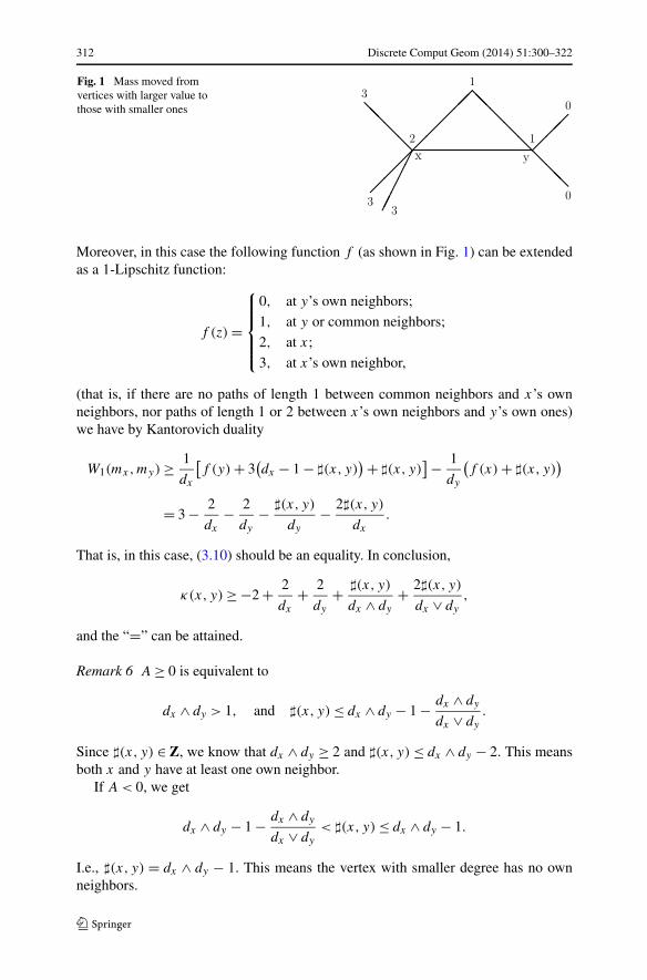
Fig. 1 Mass moved fromvertices with larger value tothose with smaller ones

Moreover, in this case the following function f (as shown in Fig. 1) can be extendedas a 1-Lipschitz function:

f (z) =

⎧⎪⎪⎪⎨

⎪⎪⎪⎩

0, at y’s own neighbors;

1, at y or common neighbors;

2, at x;

3, at x’s own neighbor,

(that is, if there are no paths of length 1 between common neighbors and x’s ownneighbors, nor paths of length 1 or 2 between x’s own neighbors and y’s own ones)we have by Kantorovich duality

W1(mx,my) ≥ 1

dx

[f (y) + 3

(dx − 1 − �(x, y)

) + �(x, y)] − 1

dy

(f (x) + �(x, y)

)

= 3 − 2

dx

− 2

dy

− �(x, y)

dy

− 2�(x, y)

dx

.

That is, in this case, (3.10) should be an equality. In conclusion,

κ(x, y) ≥ −2 + 2

dx

+ 2

dy

+ �(x, y)

dx ∧ dy

+ 2�(x, y)

dx ∨ dy

,

and the “=” can be attained.

Remark 6 A ≥ 0 is equivalent to

dx ∧ dy > 1, and �(x, y) ≤ dx ∧ dy − 1 − dx ∧ dy

dx ∨ dy

.

Since �(x, y) ∈ Z, we know that dx ∧ dy ≥ 2 and �(x, y) ≤ dx ∧ dy − 2. This meansboth x and y have at least one own neighbor.

If A < 0, we get

dx ∧ dy − 1 − dx ∧ dy

dx ∨ dy

< �(x, y) ≤ dx ∧ dy − 1.

I.e., �(x, y) = dx ∧ dy − 1. This means the vertex with smaller degree has no ownneighbors.


• A < 0 ≤ B . In this case we cannot realize step (1) but step (2) can be realized.By the above remark, A < 0 implies that y has no own neighbors. Our transfer planshould be step (2) at first. Since B ≥ 0 also implies

1 − 1

dy

− �(x, y)

dx

≥ 1

dx

, (3.11)

so we can move the mass of 1dx

at y for distance 1 to common neighbors. Finally, wefill the gap at common neighbors for distance 2. In a formula,

W1(mx,my) ≤ 1

dx

× 1 + 1

dy

× 1 +(

1 − 1

dx

− 1

dy

− �(x, y)

dx

)× 2

= 2 − 1

dx

− 1

dy

− 2�(x, y)

dx

.

Or in a symmetric manner,

W1(mx,my) ≤ 2 − 1

dx ∨ dy

− 1

dx ∧ dy

− 2�(x, y)

dx ∨ dy

. (3.12)

Moreover, in case the following function f can be extended as a 1-Lipschitz one,

f (z) =

⎧⎪⎨

⎪⎩

0, at common neighbors;

1, at x and y;

2, at x’s own neighbor,

(that is, if there are no paths of length 1 between common neighbors and x’s ownneighbors) we have by Kantorovich duality

W1(mx,my) ≥ 1

dx

[f (y) + 2

(dx − 1 − �(x, y)

)] − 1

dy

f (x)

= 2 − 1

dx

− 1

dy

− 2�(x, y)

dx

.

In conclusion,

κ(x, y) ≥ −1 + 1

dx

+ 1

dy

+ 2�(x, y)

dx ∨ dy

,

and the “=” can be attained.

Remark 7 Noting that if �(x, y) = dx ∧ dy − 1 then B ≥ 0 is equivalent to

dx ∨ dy ≥ dx ∧ dy

dx ∧ dy − 1dx ∧ dy. (3.13)

In this case, one of dx , dy has no own neighbors, and if the other one has sufficientlymany own neighbors, B ≥ 0 will be satisfied.


• A ≤ B < 0. In this case, neither step (1) nor (2) is applicable. Also, y has no ownneighbor, and B < 0 implies that we can move all the mass at x’s own neighbors to x

at first. And then we move the mass of 1dx

at y for distance 1 to fill the gaps at x andthe common neighbors. In a formula,

W1(mx,my) ≤(

1 − �(x, y)

dx

)× 1 = 1 − �(x, y)

dx

.

Or in a symmetric way,

W1(mx,my) ≤ 1 − �(x, y)

dx ∨ dy

. (3.14)

We can find a 1-Lipschitz function

f (z) ={

0, at x and common neighbors;

1, at y and x’s own neighbors.

Then by Kantorovich duality

W1(mx,my) ≥ 1

dx

(f (y) + dx − 1 − �(x, y)

) − 1

dy

× 0

= 1 − �(x, y)

dx

.

In this case f can be extended to a 1-Lipschitz function on the graph, so we get finally

κ(x, y) = �(x, y)

dx

.

Luckily, we can write those three cases in a uniform formula. �

Remark 8 From extending f to a 1-Lipschitz function, we see that the paths oflength 1 or 2 between neighbors of x and y have an important effect on the cur-vature. That is, in addition to triangles, quadrangles and pentagons are also related toOllivier’s Ricci curvature. But polygons with more than five edges do not impact it.

Remark 9 If we see the graph G = (V ,E) as a metric measure space (G,d,m), thenthe term �(x, y)/dx ∨dy is exactly mx ∧my(G) := mx(G)− (mx −my)+(G), i.e. theintersection measure of mx and my . From a metric view, the vertices x1 that satisfyx1 ∼ x, x1 ∼ y constitute the intersection of the unit metric spheres Sx(1) and Sy(1).

From Theorem 3, we can force the curvature κ(x, y) to be positive by increasingthe number �(x, y).

Theorem 4 On a locally finite graph G = (V ,E), for any neighboring x, y, we have

κ(x, y) ≤ �(x, y)

dx ∨ dy

. (3.15)


Proof Since except for the mass at common neighbors which we need not move, theothers have to be moved for a distance at least 1, we have

W1(mx,my) ≥(

1 − �(x, y)

dx ∨ dy

)× 1. �

So if κ(x, y) > 0, then �(x, y) is at least 1. Moreover, if κ(x, y) ≥ k > 0, we have

�(x, y) ≥ �kdx ∨ dy�, (3.16)

where �a� := min{A ∈ Z|A ≥ a}, for a ∈ R.We will denote D(x) := maxy,y∼x dy . By the relation (3.7), we can get immedi-

ately

Corollary 1 The scalar curvature at x can be controlled by the local clustering co-efficient at x,

dx − 1

dx

c(x) ≥ κ(x) ≥ −2 + dx − 1

dx ∨ D(x)c(x).

Remark 10 In fact in some special cases, we can get more precise lower bounds:

κ(x) ≥

⎧⎪⎪⎨

⎪⎪⎩

−2 + 2dx

+ 2D(x)

+ [ (dx−1)dx

+ 2(dx−1)dx∨D(x)

]c(x), if A ≥ 0 for all y ∼ x;

−1 + 1dx

+ 1D(x)

+ 2(dx−1)dx∨D(x)

c(x), if A < 0 ≤ B for all y ∼ x;dx−1

dx∨D(x)c(x), if B < 0 for all y ∼ x.

3.2 Weighted Graphs

The preceding considerations readily extend to weighted graphs.

Theorem 5 On a weighted locally finite graph G = (V ,E), we have

κ(x, y) ≥ −2

(1 − wxy

dx

− wxy

dy

)

+. (3.17)

Moreover, weighted trees attain this lower bound.

Theorem 6 On a weighted locally finite graph G = (V ,E), we have

κ(x, y) ≥ −(

1 − wxy

dx

− wxy

dy

−∑

x1,x1∼x,x1∼y

wx1x

dx

∨ wx1y

dy

)

+

−(

1 − wxy

dx

− wxy

dy

−∑

x1,x1∼x,x1∼y

wx1x

dx

∧ wx1y

dy

)

+

+∑

x1,x1∼x,x1∼y

wx1x

dx

∧ wx1y

dy

.

The inequality is sharp for certain graphs.


Remark 11 Notice that the term replacing the number of triangles here satisfies

∑

x1,x1∼x,x1∼y

wx1x

dx

∧ wx1y

dy

= mx ∧ my(G).

Proof Similar to the proof of Theorem 3, we need to understand the following twoterms:

Aw := 1 − wxy

dx

− wxy

dy

−∑

x1,x1∼x,x1∼y

wx1x

dx

∨ wx1y

dy

,

Bw := 1 − wxy

dx

− wxy

dy

−∑

x1,x1∼x,x1∼y

wx1x

dx

∧ wx1y

dy

.

Only the transfer plan in the case Aw < 0 ≤ Bw needs a more careful discussion. �

Theorem 7 On a weighted locally finite graph G = (V ,E), we have for any neigh-boring x, y

κ(x, y) ≤∑

x1,x1∼x,x1∼y

wx1x

dx

∧ wx1y

dy

. (3.18)

4 Curvature-Dimension Inequalities

In this section, we establish curvature-dimension inequalities on locally finite graphs.A very interesting one is the inequality under the condition κ ≥ k > 0. Curvature-dimension inequalities on locally finite graphs are studied in Lin–Yau [21]. We firststate a detailed version of their results. Let us denote Dw(x) := maxy,y∼x

dy

wyx. Notice

that on an unweighted graph, this is the D(x) we used in Sect. 3.

Theorem 8 On a weighted locally finite graph G = (V ,E), the Laplace operator �

satisfies

Γ2(f,f )(x) ≥ 1

2

(�f (x)

)2 +(

2

Dw(x)− 1

)Γ (f,f )(x). (4.1)

Remark 12 Since in this case we attach the measure (2.1), we get

Hf(x) = 1

4

1

dx

∑

y,y∼x

wxy

dy

∑

z,z∼y

wyz

(f (x) − 2f (y) + f (z)

)2.

We only need to choose special z = x in the second sum and then (2.8) and (2.9)imply the theorem.


4.1 Unweighted Graphs

We again restrict ourselves to unweighted graphs.We observe that the existence of triangles causes cancelations in calculating the

term Hf(x). This gives

Theorem 9 On a locally finite graph G = (V ,E), the Laplace operator satisfies

Γ2(f,f )(x) ≥ 1

2

(�f (x)

)2 +(

1

2t (x) − 1

)Γ (f,f )(x), (4.2)

where

t (x) := miny,y∼x

(4

dy

+ 1

D(x)�(x, y)

).

Remark 13 Notice that if there is a vertex y, y ∼ x, such that �(x, y) = 0, this willreduce to (4.1).

Proof Starting from (2.9), the main work is to compare Hf(x) with

Γ (f,f )(x) = 1

2

1

dx

∑

y,y∼x

(f (y) − f (x)

)2.

First we try to write out Hf(x) as

Hf(x) = 1

4

1

dx

∑

y,y∼x

[4

dy

(f (x) − f (y)

)2 + 1

dy

∑

z,z∼y,z �=x

(f (x) − 2f (y) + f (z)

)2].

If there is a vertex x1 which satisfies x1 ∼ x, x1 ∼ y, we have

1

dy

(f (x) − 2f (y) + f (x1)

)2 + 1

dx1

(f (x) − 2f (x1) + f (y)

)2

≥ 1

D(x)

[(f (x) − f (y)

)2 + (f (y) − f (x1)

)2 + 2(f (x) − f (y)

)(f (x1) − f (y)

)

+ (f (x) − f (x1)

)2 + (f (y) − f (x1)

)2 + 2(f (y) − f (x1)

)(f (x) − f (x1)

)]

= 1

D(x)

[(f (x) − f (y)

)2 + 4(f (y) − f (x1)

)2 + (f (x) − f (x1)

)2]

≥ 1

D(x)

(f (x) − f (y)

)2. (4.3)

So the existence of a triangle which includes x and y will give another term

1

D(x)

(f (y) − f (x)

)2


to the sum in Hf(x). Since this effect is symmetric w.r.t. y and x1, we can get

Hf(x) ≥ 1

4

1

dx

∑

y,y∼x

(4

dy

+ 1

D(x)�(x, y)

)(f (y) − f (x)

)2

≥ t (x)1

4

1

dx

∑

y,y∼x

(f (y) − f (x)

)2

= t (x) · 1

2Γ (f,f )(x).

Inserting this into (2.9) completes the proof. �

Recalling Theorem 4 and the subsequent discussion, we get the followingcurvature-dimension inequalities on graphs with positive Ollivier–Ricci curvature.

Corollary 2 On a locally finite graph G = (V ,E), if κ(x, y) > 0, then we have

Γ2(f,f )(x) ≥ 1

2

(�f (x)

)2 +(

5

2D(x)− 1

)Γ (f,f )(x). (4.4)

Corollary 3 On a locally finite graph G = (V ,E), if κ(x, y) ≥ k > 0, then we have

Γ2(f,f )(x) ≥ 1

2

(�f (x)

)2

+(

1

2min

y,y∼x

{4

dy

+ �kdx ∨ dy�D(x)

}− 1

)Γ (f,f )(x). (4.5)

Remark 14 Observe that a rough inequality in this case is

Γ2(f,f )(x) ≥ 1

2

(�f (x)

)2 +(

2

D(x)+ kdx

2D(x)− 1

)Γ (f,f )(x).

Comparing this one with (4.1), we see that positive κ increases the curvature functionhere.

Remark 15 We point out that the condition κ(x, y) ≥ k > 0 implies that the diameterof the graph is bounded by 2

k(see Proposition 23 in Ollivier [24]). So in this case the

graph is a finite one.

Let us revisit the example of a complete graph Kn (n ≥ 2) with n vertices. Recallin Example 1, we know

κ(x, y) = n − 2

n − 1, ∀x, y.


For the curvature-dimension inequality on Kn, Theorem 9 or Corollary 3 using theabove κ implies

Γ2(f,f ) ≥ 1

2(�f )2 +

(2

n − 1− 1 + 1

2

n − 2

n − 1

)Γ (f,f )

= 1

2(�f )2 + 4 − n

2(n − 1)Γ (f,f ). (4.6)

Moreover, the curvature term in the above inequality cannot be larger. To see this, wecalculate, using the same trick as in (4.3),

Hf(x) = 1

4(n − 1)2

∑

y,y∼x

∑

z,z∼x

(f (x) − 2f (y) + f (z)

)2

= n + 2

2(n − 1)Γ (f,f )(x) + 1

(n − 1)2

∑

(x1,x2)

(f (x1) − f (x2)

)2,

where∑

(x1,x2)means the sum over all unordered pairs of neighbors of x. Recalling

(2.9), we get

Γ2(f,f )(x) = 1

2(�f )2(x) + 4 − n

2(n − 1)Γ (f,f )(x)

+ 1

(n − 1)2

∑

(x1,x2)

(f (x1) − f (x2)

)2. (4.7)

For any vertex x, we can find a particular function f ,

f (z) ={

2, when z = x;

1, when z ∼ x,(4.8)

such that the last term in (4.7) vanishes, and Γ (f ,f ) �= 0. This means the curvatureterm in (4.6) is optimal for dimension parameter 2.

But the curvature term 4−n2(n−1)

behaves very differently from κ . In fact as n → +∞,

4 − n

2(n − 1)↘ −1

2whereas κ ↗ 1.

To get a curvature-dimension inequality with a curvature term which behaveslike κ , it seems that we should adjust the dimension parameter. In fact, we have

Proposition 3 On a complete graph Kn (n ≥ 2) with n vertices, the Laplace operator� satisfies for m ∈ [1,+∞],

Γ2(f,f )(x) ≥ 1

m

(�f (x)

)2 +(

4 − n

2(n − 1)+ m − 2

m

)Γ (f,f )(x). (4.9)

Moreover, for every fixed dimension parameter m, the curvature term is optimal.


Proof We have from (4.7)

Γ2(f,f )(x) = 1

m(�f )2(x) + 4 − n

2(n − 1)Γ (f,f )(x)

+ 1

(n − 1)2

∑

(x1,x2)

(f (x1) − f (x2)

)2 +(

1

2− 1

m

)(�f )2.

Let us denote the sum of the last two terms by I . Then we have

I = 1

(n − 1)2

{(1

2− 1

m

) ∑

y,y∼x

(f (y) − f (x)

)2

+∑

(x1,x2)

[(f (x1) − f (x)

)2 + (f (x2) − f (x)

)2

+(

2

(1

2− 1

m

)− 2

)(f (x1) − f (x)

)(f (x2) − f (x)

)]}

= 1

(n − 1)2

[(1

2− 1

m

) ∑

y,y∼x

(f (y) − f (x)

)2

+(

1 − m + 2

2m

)(n − 2)

∑

y,y∼x

(f (y) − f (x)

)2

+∑

(x1,x2)

m + 2

2m

(f (x1) − f (x2)

)2]

= m − 2

mΓ (f,f )(x) + m + 2

2m(n − 1)2

∑

(x1,x2)

(f (x1) − f (x2)

)2.

This finishes the proof. �

An interesting point appears when we choose the dimension parameter m of Kn

as n − 1. Then we have

Γ2(f,f ) ≥ 1

n − 1(�f )2 + 1

2

n − 2

n − 1Γ (f,f ),

where the curvature term is exactly 12κ . From the fact that Kn could be considered

as the boundary of a (n − 1) dimensional simplex, the m we choose here seems alsonatural.

Remark 16 We point out another similar fact here. On a locally finite graph withmaximal degree D and minimal degree larger than 1, Theorem 2 and Theorem 8imply that

κ(x, y) ≥ 2

(2

D− 1

), ∀x, y, (4.10)


and

Γ2(f,f ) ≥ 1

2(�f )2 +

(2

D− 1

)Γ (f,f ), (4.11)

respectively. It is not difficult to see that for regular trees with degree larger than 1,the curvature term in (4.11) is optimal. (Just consider the extension of the function(4.8), taking values 0 on vertices which are not x and neighbors of x there.) So onregular trees, the curvature term is also exactly 1

2κ .

Remark 17 In Erdös–Harary–Tutte [15], they define the dimension of a graph G asthe minimum number n such that G can be embedded into a n dimensional Euclideanspace with every edge of G having length 1. It is interesting that by their definition,the dimension of Kn is also n − 1 and the dimension of any tree is at most 2.

From the above observations, it seems natural to expect stronger relations betweenthe lower bound of κ and the curvature term in the curvature-dimension inequality ifone chooses proper dimension parameters.

4.2 Weighted Graphs

We have similar results on weighted graphs here, with similar proofs.

Theorem 10 On a weighted locally finite graph G = (V ,E), the Laplace operatorsatisfies

Γ2(f,f )(x) ≥ 1

2

(�f (x)

)2 +(

1

2tw(x) − 1

)Γ (f,f )(x), (4.12)

where

tw(x) := miny,y∼x

{4wxy

dy

+∑

x1,x1∼x,x1∼y

(wxy

dy

∧ wxx1

dx1

)wx1y

wxy

}.

Acknowledgements The research leading to these results has received funding from the European Re-search Council under the European Union’s Seventh Framework Programme (FP7/2007-2013)/ERC grantagreement n◦267087.

We thank Persi Diaconis for pointing out Ollivier’s notion of Ricci curvature to us.

References

1. Bakry, D.: Functional inequalities for Markov semigroups. In: Dani, S.G., Graczyk, P. (eds.) Proba-bility Measures on Groups: Recent Directions and Trends, pp. 91–147. Tata, Bombay (2006)

2. Bakry, D., Émery, M.: Diffusions hypercontractives. In: Azéma, J., Yor, M. (eds.) Séminaire de prob-abilités, XIX. Lecture Notes in Math., vol. 1123, p. 177–206. Springer, Berlin (1985)

3. Bakry, D., Émery, M.: Hypercontractivité de semi-groupes de diffusion. C. R. Math. Acad. Sci. 299,775–778 (1984)

4. Banerjee, A., Jost, J.: On the spectrum of the normalized graph Laplacian. Linear Algebra Appl. 428,3015–3022 (2008)

5. Bauer, F., Jost, J.: Bipartite and neighborhood graphs and the spectrum of the normalized graph Lapla-cian. Commun. Anal. Geom. 21(4), 787–845 (2013). doi:10.4310/CAG.2013.v21.n4.a2

http://dx.doi.org/10.4310/CAG.2013.v21.n4.a2


6. Bauer, F., Jost, J., Liu, S.: Ollivier–Ricci curvature and the spectrum of the normalized graph Laplaceoperator. Math. Res. Lett. 19(6), 1185–1205 (2012). doi:10.4310/MRL.2012.v19.n6.a2

7. Bonciocat, A.-I., Sturm, K.-T.: Mass transportation and rough curvature bounds for discrete spaces. J.Funct. Anal. 256, 2944–2966 (2009)

8. Chung, F.R.K.: Spectral Graph Theory. CBMS Regional Conference Series in Mathematics, vol. 92.Am. Math. Soc., Providence (1997)

9. Chung, F.R.K., Yau, S.T.: Logarithmic Harnack inequalities. Math. Res. Lett. 3, 793–812 (1996)10. Diaconis, P., Stroock, D.: Geometric bounds for eigenvalues of Markov chains. Ann. Appl. Probab. 1,

36–61 (1991)11. Diaconis, P., Saloff-Coste, L.: Logarithmic Sobolev inequalities for finite Markov chains. Ann. Appl.

Probab. 6, 695–750 (1996)12. Diaconis, P.: From shuffling cards to walking around the building: an introduction to modern Markov

chain theory. In: Proceedings of the International Congress of Mathematicians, Vol. I. Doc. Math., pp.187–204 (1998)

13. Diaconis, P.: The Markov chain Monte Carlo revolution. Bull., New Ser., Am. Math. Soc. 46, 179–205(2009)

14. Dodziuk, J., Karp, L.: Spectral and Function Theory for Combinatorial Laplacians. Contemp. Math.,vol. 73. Amer. Math. Soc., Providence (1988)

15. Erdös, P., Harary, F., Tutte, W.T.: On the dimension of a graph. Mathematika 12, 118–122 (1965)16. Evans, L.C.: Partial differential equations and Monge–Kantorovich mass transfer. In: Bott, R., Jaffe,

A., Jerison, D., Lusztig, G., Yau, S.T. (eds.) Current Developments in Mathematics, pp. 65–126. In-ternational Press, Boston (1999)

17. Forman, R.: Bochner’s method for cell complexes and combinatorial Ricci curvature. Discrete Com-put. Geom. 29, 323–374 (2003)

18. Jost, J.: Riemannian Geometry and Geometric Analysis, 6th edn. Springer, Berlin (2011)19. Lin, Y.: Ricci curvature on graphs. John H. Barrett Memorial Lecture (2010). http://www.math.utk.

edu/barrett/2010/talks/YongLinRicci.pdf20. Lin, Y., Lu, L., Yau, S.T.: Ricci curvature of graphs. Tohoku Math. J. 63, 605–627 (2011)21. Lin, Y., Yau, S.T.: Ricci curvature and eigenvalue estimate on locally finite graphs. Math. Res. Lett.

17, 343–356 (2010)22. Lott, J., Villani, C.: Ricci curvature for metric measure spaces via optimal transport. Ann. Math. 169,

903–991 (2009)23. Ohta, S.-I.: On the measure contraction property of metric measure spaces. Comment. Math. Helv.

82, 805–828 (2007)24. Ollivier, Y.: Ricci curvature of Markov chains on metric spaces. J. Funct. Anal. 256, 810–864 (2009)25. Ollivier, Y.: A survey of Ricci curvature for metric spaces and Markov chains. In: Kotani, M., Hino,

M., Kumagai, T. (eds.) Probabilistic Approach to Geometry. Adv. Stud. Pure Math., vol. 57, pp. 343–381. Math. Soc. Japan, Tokyo (2010)

26. Ollivier, Y., Villani, C.: A curved Brunn–Minkowski inequality on the discrete hypercube. SIAM J.Discrete Math. 26(3), 983–996 (2012). doi:10.1137/11085966X

27. Paeng, S.-H.: Volume, diameter of a graph and Ollivier’s Ricci curvature. Eur. J. Comb. 33(8), 1808–1819 (2012). doi:10.1016/j.ejc.2012.03.029

28. Stone, D.A.: A combinatorial analogue of a theorem of Myers. Ill. J. Math. 20, 12–21 (1976). Correc-tion: Ill. J. Math. 20, 551–554 (1976)

29. Sturm, K.-T.: On the geometry of metric measure spaces. I. Acta Math. 196, 65–131 (2006)30. Sturm, K.-T.: On the geometry of metric measure spaces. II. Acta Math. 196, 133–177 (2006)31. Villani, C.: Topics in Optimal Transportation. Graduate Studies in Mathematics, vol. 58. Am. Math.

Soc., Providence (2003)32. Villani, C.: Optimal Transport, Old and New. Grundlehren der Mathematischen Wissenschaften,

vol. 338. Springer, Berlin (2009)33. Watts, D.J., Strogatz, S.H.: Collective dynamics of ‘small-world’ networks. Nature 393, 440–442

(1998)

http://dx.doi.org/10.4310/MRL.2012.v19.n6.a2

http://www.math.utk.edu/barrett/2010/talks/YongLinRicci.pdf

http://www.math.utk.edu/barrett/2010/talks/YongLinRicci.pdf

http://dx.doi.org/10.1137/11085966X

http://dx.doi.org/10.1016/j.ejc.2012.03.029

ollivier’s ricci curvature, local clustering and curvature ...ollivier’s ricci curvature, local...

Documents