offshoring and productivity revisited: a time-series analysisftp.iza.org/dp7323.pdf · offshoring...

DI

SC

US

SI

ON

P

AP

ER

S

ER

IE

S

Forschungsinstitut zur Zukunft der ArbeitInstitute for the Study of Labor

Offshoring and Productivity Revisited:A Time-Series Analysis

IZA DP No. 7323

March 2013

Pablo Agnese

Offshoring and Productivity Revisited:

A Time-Series Analysis

Pablo Agnese FH Düsseldorf

and IZA

Discussion Paper No. 7323 March 2013

IZA

P.O. Box 7240 53072 Bonn

Germany

Phone: +49-228-3894-0 Fax: +49-228-3894-180

E-mail: [email protected]

Any opinions expressed here are those of the author(s) and not those of IZA. Research published in this series may include views on policy, but the institute itself takes no institutional policy positions. The IZA research network is committed to the IZA Guiding Principles of Research Integrity. The Institute for the Study of Labor (IZA) in Bonn is a local and virtual international research center and a place of communication between science, politics and business. IZA is an independent nonprofit organization supported by Deutsche Post Foundation. The center is associated with the University of Bonn and offers a stimulating research environment through its international network, workshops and conferences, data service, project support, research visits and doctoral program. IZA engages in (i) original and internationally competitive research in all fields of labor economics, (ii) development of policy concepts, and (iii) dissemination of research results and concepts to the interested public. IZA Discussion Papers often represent preliminary work and are circulated to encourage discussion. Citation of such a paper should account for its provisional character. A revised version may be available directly from the author.

mailto:[email protected]

IZA Discussion Paper No. 7323 March 2013

ABSTRACT

Offshoring and Productivity Revisited: A Time-Series Analysis*

The subject of offshoring and productivity has not yet received the attention it deserves. Here I propose a simple framework for estimating the contribution of these strategies to the growth rate of labor productivity from a time-series perspective. This framework is then used to assess the impact of offshoring on skill upgrading and the labor share. For both empirical questions I take up the study of a group of Japanese industries during the recent years of slow growth. The results should be interpreted with caution yet clearly suggest that offshoring can improve labor productivity in the Semiconductors industry. Moreover, offshoring is found to be the source of important changes among industries with different skills (skill upgrading) and an important factor behind the fall of the labor share. JEL Classification: J23, J24, E25 Keywords: offshoring, labor productivity, skill upgrading, labor share Corresponding author: Pablo Agnese FH Düsseldorf Department of Business Studies Universitätsstraße, Gebäude 23.32 40225 Düsseldorf Germany E-mail: [email protected]

* I am thankful for financial support received from Fundacion BBVA through project grant 162-06.

mailto:[email protected]

1 Introduction

Much has been said about o¤shoring and its employment e¤ects� which might seem

at times to be quite ambiguous. Far less, however, has been said on the productivity

e¤ects. Here we will take up the up the study of o¤shoring and productivity using a

time-series perspective for the industry, something on which the literature has not yet

produced a clear consensus. To achieve this I will take a look at a major event in the

Japanese economy: the �lost decade�� that period of economic contraction which spans

from somewhere in the 1990s to present days, and which is characterized by a slowdown

of the growth rate of productivity. With this landscape in mind, our main objective

will be to assess the impact of o¤shoring strategies on the performance of industries.

I will propose a simple model whereby it will be possible to derive the net e¤ect

of o¤shoring on the growth rate of labor productivity for di¤erent industries. This

�rst empirical exercise will simulate the growth rate of labor productivity after the

East Asian crisis (1997) assuming that the o¤shoring strategies remained unchanged at

that initial level. Considering that over the last few years the o¤shoring of Japanese

activities has really leaped forward (see Agnese, 2012), then it is of interest to see

whether these activities may have prevented a more pronounced downturn of economic

activity.1 A second empirical exercise will look upon o¤shoring as a source of skill-

biased technological change, in the sense that these managerial strategies can lead to

skill upgrading as well as to changes in the industry�s labor share. Given that the labor

share has been falling in most of the developed world, it will be useful to see how much

o¤shoring has contributed to that change in Japan.

The Japan Industrial Productivity (JIP) Database (RIETI, 2011) will provide the

data on a vast number of economic activities classi�ed as 108 industries, out of which we

will be using four for reasons that will become clear below. Our main results, which are

in line with the recent literature, point to the existence of positive e¤ects of o¤shoring

on the growth rate of labor productivity for some of the industries (see Amiti and

Wei, 2009, for the US, Girma and Görg, 2004, for the UK, and Hijzen et al., 2010, for

Japan). Our second set of results suggests that o¤shoring can be seen as a source of

skill-biased technological change because of, �rst, the presence of skill upgrading (e.g.

high-skill workers see their wages increase due to higher productivity) and, second, the

negative e¤ect of o¤shoring on the labor share (e.g. �rms resources from labor to more

capital-intensive activities).2

1The recent Japanese experience is very well documented in several places and from di¤erent angles(see Caballero et al., 2008, Fukao and Kwon, 2006, Hayashi and Prescott, 2002, or Krugman, 1998,among many others).

2References on skill upgrading abound (see, among several others, Berman et al., 1994, and Feenstraand Hanson, 1996, for the US, Geishecker and Görg, 2005, for Germany, Head and Ries, 2002, for Japan,or Hijzen et al., 2005, for the UK). I am unaware, however, of any studies on the relationship between

2

The industries I will be focusing on are classi�ed by the JIP Database as informa-

tion technology (IT) manufacturing industries. Table 1 condenses some comparative

information on the broad sectors within the database for which data were available

(1976�2008), and shows that IT-Manufacturing industries are traditionally more pro-

ductive. Even when all sectors have been hardly hit by the slump, the IT-Manufacturing

sector has still managed to fare reasonably well.

Table 1: Labor productivity growth rate, broad sector averages (%).

1976-2008 1976-1980 1981-1990 1991-2000 2001-2008

IT-Manufacturing 5.81 8.14 9.51 3.40 2.73

IT 4.32 5.99 6.68 3.21 1.73

Manufacturing 3.53 6.24 6.86 2.19 -0.63

All 2.80 3.68 4.69 2.78 -0.09

Source (all tables and �gures): JIP Database (RIETI, 2011), own calculations.

Figure 1 complements the previous information and shows more in detail the down-

ward trend of labor productivity for the same broad sectors. This general decline in the

performance of the economy was severely felt especially after the 1997 crisis, when the

growth rate of labor productivity stood at negative levels for many of the years that

followed.

Figure 1. Labor productivity growth rate, broad sector averages (%).

12

8

4

0

4

8

12

16

20

24

1980 1985 1990 1995 2000 2005

Avg ITManufacturingAvg ITAvg ManufacturingAvg all

a. Waning growth, 19762008

Asian crisis (1997)

12

8

4

0

4

8

12

97 98 99 00 01 02 03 04 05 06 07 08

Avg ITManufacturingAvg ITAvg ManufacturingAvg all

b. The aftermath of the Asian crisis, 19972008

Since IT-Manufacturing industries were the least a¤ected by the sti�ing economic

conditions during the aftermath of the Asian crisis, we might want to know whether

the industries there do share some speci�c trait that could explain their not so bad per-

formances. IT industries are at the front of innovation and technological developments;

o¤shoring and the labor income share.

3

o¤shoring, in particular, can be thought of as a managerial innovation whereby �rms,

as with any other technological improvement, can become more e¢ cient. We need now

to measure o¤shoring before going any further.

Feenstra and Hanson (1996) �rst de�ned o¤shoring as the share of imported inter-

mediate inputs in the total purchase of nonenergy inputs:

osit =IitQt

�itDit

where Ii is purchases of inputs i by industry i, Q is total inputs (excluding energy)

used by i, �i is total imports of good i, and Di its domestic demand. This is a narrow

de�nition of o¤shoring for it only accounts for the intermediate inputs that �rms within

industry i import from foreign �rms in the same industry. I think this narrow measure

makes for a better choice when using aggregate industry-level data, as it will diminish

the aggregation-o¤shoring bias (on this issue see Fukao and Arai, 2013). Moreover, the

�rst term in the de�nition above generally stems from the census data or Input-Output

tables, while the second term, an economy-wide import share, is obtained from trade

data. In our case, though, given that the data are taken from the same source, it is to

expect that the measurement errors underlying the whole endeavor will be signi�cantly

reduced.

Figure 2. O¤shoring intensity and IT-Manufacturing (%).

0.5

1.0

1.5

2.0

2.5

3.0

3.5

4.0

1980 1985 1990 1995 2000 2005

ITManufacturing (avg.)ITManufacturing + other (avg.)

a. In perspective, 19762008

0

2

4

6

8

10

12

1980 1985 1990 1995 2000 2005

SemiconductorsElectronic partsIndustry machineryElectronic equipmentITManufacturing (avg.)

b. Selected industries, 19762008

To drive the point home we need to highlight the trend of o¤shoring intensity of

IT-Manufacturing industries among the most representative ones3 within the database.

3Among these were some non-IT Manufacturing and some IT non-Manufacturing. Note that highlydeveloped industries, while being exposed to new technologies more rapidly, can also engage in whathas come to be known as �services�o¤shoring. The use of a narrow measure of o¤shoring prevents usfrom further breaking down the data into �materials�and �services o¤shoring�, as it is sometimes done(see, for instance, Amiti and Wei, 2009, for the US, or Ito and Tanaka, 2010, for Japan).

4

Figure 2a shows an important di¤erence regarding these strategies. Furthermore, Figure

2b zooms in on a small set of IT-Manufacturing industries that show di¤erent trends.

Two of these industries, Semiconductors and Electronic Parts, are distinctly above the

sector�s average, whereas the other two, Industry machinery and Electronic equipment,

are clearly below. Seemingly, highly productive IT-Manufacturing industries can have

very di¤erent o¤shoring strategies.

With the exception of Industry machinery, the industries show a high growth rate

of labor productivity during the post-crisis years (1997�present). It is left to wonder if

o¤shoring might have had anything to do with these their experiences. In addition, we

might want to know if o¤shoring played any role in the major changes that took place

during those years (e.g. a signi�cant drop in the labor income share).

The paper is organized as follows. Section 2 re�ects on the decision to favor a

time-series study instead of panel data analysis, and then goes over the details of the

model. Section 3 discusses the data and methodology, shows the estimation of the model

for the four industries discussed earlier, and then o¤ers the diagnosis of our empirical

analysis. Section 4 uses the models from the previous section to produce two dynamic

accounting exercises regarding the e¤ects of o¤shoring on productivity and the labor

share; this section also o¤ers some remarks on the possibility of skill upgrading. Section

5 concludes.

2 Empirical framework

2.1 To pool or not to pool?

The o¤shoring phenomenon is now under thorough examination within the academic

�eld, with the majority of empirical work being conducted at the �rm level.4 Due to the

dimensions of these databases it is generally useful to pool the information somehow

and estimate the e¤ects on the average �rm. This heterogeneity usually implies the

use of GMM-type estimators, which can capture the di¤erences among cross-sections

more e¢ ciently than pooled estimators and, at the same time, can address the potential

endogeneity of the o¤shoring variable.

The JIP Database (RIETI, 2011), however, only collects industry level data for a

wide set of activities in 108 Japanese industries. The natural strategy would be to pool

all industries so as to estimate the e¤ects on the average industry, just as is done for

the �rm. But when it comes to industry data we should be aware of the aggregation

problem; that is, even when �rms can be very di¤erent within the same industry, it is

even more likely that these di¤erences are more pronounced across industries. Under

4This is true for most of the references cited in the Introduction and footnote 2.

5

these circumstances it will be more interesting to focus separately on the four IT-

Manufacturing industries presented in the introduction while adopting a time-series

perspective. In addition, industry-level data, as opposed to �rm data, allows for an

easier interpretation of the labor share e¤ects of o¤shoring� something on which the

literature has yet to provide some answers.

Firms in highly developed industries like the ones involved in this study do share

several characteristics. Most of these characteristics come from the technological side,

but some of them stem from the human resource management practices (see for instance

Tsai, 2010, for the semiconductor industry). The point is that within each of the four

industries we want to look into, there is a high degree of homogeneity as to downplay the

possible aggregation bias5 which is inherent to these studies. Of course, o¤shoring must

still be instrumented as to address the endogeneity as in the case of panel estimation.

The next section presents a simple setting that will be later used to carry out our

dynamic accounting exercises.

2.2 A simple model

Here I propose a simple model that I will later use to track down the possible e¤ects of

o¤shoring on productivity growth. For this purpose I assume a Cobb-Douglas produc-

tion function as below:

Y = A (os)K�N1�� (1)

where Y is the output supplied by the �rm, K its stock of capital, N its employment

level, � and 1�� the input elasticities,6 and A the technology shifter� which is depen-dent on the o¤shoring index as de�ned above and satis�es that A0(os) > 0, as o¤shoring

can increase productivity in numerous ways (more on this below).

The marginal productivities in this case are given by:

MPK =@Y

@K= �A (os)K��1N1�� (2)

MPN =@Y

@N= (1� �)A (os)K�N�� (3)

Costs are de�ned as usual, as the total expenditures on inputs:

C = RK +WN

5The use of a narrow o¤shoring index, as explained earlier, contributes too in this direction.6For reasons of exposition I will stick to the constant returns to scale hypothesis, but this should

not be necessarily so. I will get back to this point later.

6

where R and W are the input prices, real interest rate and real average wages. Cost

minimization, given a certain level of output, determines that the ratio of marginal

productivities be equal to the ratio of factor prices, that is MPNMPK

= WR. Expressing

the latter as �MPNMPK

= �WRimplies that the slope of the isoquant (e.g. the marginal

rate of substitution) and isocost are both equal. From the cost de�nition above we

know that K =�CR

��WR

�N and @K

@N= �

�WR

�, and from (2) and (3) we know that

�MPNMPK

= �h(1��)�

KN

i. Finally, the cost minimization equilibrium condition is, as always:

��(1� �)�

K

N

�= �

�W

R

�From here it is possible to derive the conditional factor demand for both capital

and labor. Clearing up N in the equilibrium condition above we get N = (1��)�

RWK,

which we plug then into (1) to obtain the conditional factor demand for capital K =hA (os)�1

��1��1�� W

R

�1��iY . To obtain the conditional factor demand for labor we

substitute the last expression into (1), which yields the following symmetrical expres-

sion:

N =

�A (os)�1

�1� ��

��R

W

��Y (4)

where employment is dependent, among other things, on the o¤shoring intensity index.

Aggregating (1) and (4) to the industry level, taking logs, and adding lags, errors,

and the time subscript, we get an estimable system which is useful for tracking down

the e¤ects of o¤shoring on the industry�s labor productivity:

yt = �1 + �1yt�1 + �1nt + �kt + �1ost + "1 (5)

nt = �2 + �2nt�1 + wt + �2yt + �2ost + "2 (6)

�t ' yt � nt (7)

where the small letters are the variables in logs with their corresponding coe¢ cients,

to wit: �1 and �2 the output and employment inertia coe¢ cients,7 �1 and � the em-

ployment and capital elasticities to output, the wage elasticity to employment, �1and �2 the o¤shoring semi-elasticities, and "1 and "2 the normally distributed errors

with constant variance. Finally, let � be the productivity of labor, which is de�ned as

the ratio of output to the labor input. Since both output and labor are expressed in

7Introducing dynamics here allows us to conceive the existence of some frictions within the labormarket. For the labor demand in particular, these can be interpreted as the adjustment costs employersface when signi�cant training and �ring costs are present� and these frictions are consistent with thepresence of involuntary unemployment which, in turn, are an expected outcome of o¤shoring practicesfor some workers.

7

logarithms we can approximate labor productivity by (7)� and then track down the

changes in � (��) as we set out to do originally.

I also expect the following signs for the coe¢ cients: 0 < �1 < 1, 0 < �2 < 1, as

to guarantee dynamic stability,8 �1 > 0 and � > 0,9 < 0 (a negatively sloped labor

demand), �2 > 0, and �1 > 0 and �2 < 0. On the latter two coe¢ cients a few remarks

are in order.

Amiti and Wei (2009) identify four possible channels through which o¤shoring can

a¤ect productivity: (i) static e¢ ciency gain, (ii) restructuring, (iii) learning externali-

ties, and (iv) variety e¤ects. First, when �rms decide to relocate activities to overseas

locations they relocate the less e¢ cient parts and average productivity increases due

to a compositional e¤ect. Second, the remaining workers may become more e¢ cient if

�rms can restructure in a way that pushes out the technology frontier. Third, �rms can

learn to improve the way activities are performed by importing services. And fourth,

productivity could increase due to the use of new material or service input varieties.

The model above cannot distinguish the exact channel of the productivity gain arising

from o¤shoring, yet we can assume that these are embedded into �1 and �2.

3 Empirical analysis

3.1 Data and methodology

The data I use for this study come from the JIP Database (RIETI, 2011), ranging

from 1970 to 2008 and including 108 industries from di¤erent branches of economic

activity� services and manufacturing being the main categories. The four industries

under study are categorized as both manufacturing and IT-intensive industries.

8For a dynamic model of the type:

A0yt =nXi=1

Aiyt�i +nXi=0

Dixt�i + "t;

where yt is a vector of endogenous variables, xt a vector of exogenous variables, Ai�s and Di�s arecoe¢ cient matrices, and "t a vector of strict white noise error terms; then the dynamic system aboveis stable if, for given values of the exogenous variables, all the roots of the determinantal equation(where B is the backshift operator)

jA0 �A1B:::�AnBnj = 0

lie outside the unit circle. The estimated equations below satisfy this condition.9The constant returns to scale hypothesis would require that �1

(1��2)+ �(1��2)

= 1: Notice that downbelow I do not constrain the equations as to ful�ll this hypothesis (the estimation results are not thatdi¤erent from one another anyhow). Non-constant returns would imply that (1) and (4) should beslightly changed but this is of no real importance for the empirical analysis below.

8

Table 2: Summary statistics, 1976-2008.

Industry / Variable Mean Max. Min. Std. dv.

Semiconductors

N : employment (workers) 145,192 236,251 7,252 80,217

W : average real wages (million yen) 4.12 16.46 1.06 3.38

Y : real output (million yen) 1,245,543 4,274,040 14,160 1,145,483

K : real net capital stock (million yen) 4,715,221 12,665,640 402,851 3,764,188

os : o¤shoring index (%) 2.28 11.57 0.04 3.45

�� : labor productivity growth rate (%) 9.58 77.24 -33.93 18.85

Electronic parts



Y : real output (million yen) 2,412,535 6,686,689 240,717 1,769,861

K : real net capital stock (million yen) 2,928,973 6,185,476 526,448 1,994,487



Industry machinery



Y : real output (million yen) 2,819,787 3,841,516 1,550,403 642,478

K : real net capital stock (million yen) 5,594,873 9,077,593 2,217,262 2,241,890



Electronic equipment



Y : real output (million yen) 882,535 1,770,692 153,761 475,369

K : real net capital stock (million yen) 1,006,303 1,842,645 218,022 500,279



Note: 33 observations (1976-2008); Y is gross value added (at factor prices), and Y , K, and W

were de�ated using the GDP de�ator (JIP Database 2011). Variables not in logs.

Table 2 summarizes the main information on the time-series I use in the estima-

tion below. Notice that, as in all tables and �gures, the industries are ordered by

their �o¤shoring intensity�, namely: 1o semiconductors, 2o electronic parts, 3o industry

9

machinery, 4o electronic equipment.10

The estimation strategy involves the Autoregressive Distributed Lagged (ARDL)

approach by Pesaran (1997), Pesaran and Shin (1999), and Pesaran et al. (2001).

The ARDL yields consistent estimates for the short and long-run that can used when

regressors are either I(1) or I(0), as it is our case. For each industry I estimate a two-

equation system that allows me to track down the changes in labor productivity and

assess the contribution of o¤shoring.

Equations (5) and 6 are �rst estimated separately and evaluated against a set of

diagnostic tests. Both equations are then estimated jointly with the three-stage least

squares method (3SLS), which accounts for potential endogeneity and cross-equation

correlation. The potential endogeneity of some of the variables is something we should

take into consideration. In particular for the o¤shoring index, endogeneity can be

further magni�ed by the presence of measurement errors. To solve for this we instrument

wages, capital, and the o¤shoring index, with the past values of wages and capital.11

As a �nal step we should check on the validity of the long-run relationships among

the growing variables in the models. For this I reparametrize the estimated equations

as error correction models (ECMs) and obtain the cointegrating vectors (CVs) among

the I(1) variables. Even when the ECM on its own gives proof of cointegration of the

time-series involved, I also use Johansen�s cointegration procedure (Johansen, 1988)

to check whether the long-run relationships conform with those obtained through the

estimation of the two-equation model. I will get back to this later.

3.2 Estimation

Tables 3a to 3d present the two-equation models for all four industries. Note that in

all cases the coe¢ cients are properly signed (e.g. as hypothesized above), and in most

cases turn out signi�cant at conventional levels. The o¤shoring coe¢ cients, however,

turn out with a lower signi�cance and, in some cases, are non-signi�cant at all (it is

denoted with an � in the tables).12 For the Semiconductors industry they are signi�cant

10The broad economic sectors in the JIP Database correspond to the codes: 1�7 for primary in-dustries, 8�59 for manufacturing, 60�61 construction, 62�66 energy, and 67�108 services. Our fourindustries of interest are coded and fully labeled as follows: 51. Semiconductor devices and integratedcircuits; 52. Electronic parts; 50. Electronic equipment and electric measuring instruments; and 42.General industry machinery. See Appendix A for a correspondence between these four industries inthe JIP and other well-known databases and international classi�cations.11We also try with other exogenous instruments for the o¤shoring index in particular, namely: the

investment in information technology used to produce software and hardware, but the results arenot changed signi�cantly (see Appendix B). Moreover, the endogeneity of o¤shoring does not pose soserious a problem for industry level data as it does for �rm level data. Regardless, the validity of theinstruments and of the overidentifying restrictions must still be checked� this I do below by means ofa conventional Sargan test.12The dynamic structure of all four models is rather unpromising too. However, it should be stressed

that the introduction of dynamics is due to the fact that they are a source of frictions which can bring

10

at 5% in both equations (Table 3a); for the Electronic parts industry it is signi�cant

only in the production function at 5% level (Table 3b); for Industry machinery it is only

(yet highly) signi�cant in the labor demand equation, at 1% level (Table 3c); and for

Electronic equipment it is neither signi�cant in the labor demand nor in the production

function.

Because the number of instruments exceeds the number of regressors in the proposed

models we must test for the validity of the overidentifying restrictions. Under the null

hypothesis that these are valid, the Sargan statistic is distributed as �2(k�p) with k the

number of instruments and p the number of estimated coe¢ cients. Not rejecting the test

at conventional levels (e.g. above 5%) is indicative of the exogeneity of the instruments

used.13

In spite of these not totally convincing results, it should be noted that all o¤shoring

coe¢ cients are properly signed. That is, in all cases o¤shoring seems to exert a negative

impact on the demand for labor and a positive one on production. This is in agreement

with the economic intuition as pointed out before (see Amiti and Wei, 2009). Even

when our goal is to track down the changes in labor productivity that have taken place

in the past few years, it is possible here to come up with an extent of the magnitude

of the e¤ects involved in the di¤erent sectors. But for this it will be needed to get the

long-run elasticities to make the e¤ects comparable among the industries.

Table 4 shows the short and long-run elasticities for the models. Notice that we refer

to these as semi-elasticities because the o¤shoring index is not expressed in logarithms.14

The columns labeled as �SRn�os and �SRy�os correspond to the short-run semi-elasticities as

estimated in Tables 3a to 3d, while the columns labeled as �LRn�os and �LRy�os correspond

to the long-run semi-elasticities and are calculated simply as �LRn�os =�1

(1��2)and �LRy�os =

�2(1��2)

.

When it comes to "employment loss" the e¤ects are only signi�cant within Semicon-

ductors and Industry machinery, with larger e¤ects on the latter. These e¤ects should

come as no surprise since even when these industries qualify as IT, they entail di¤erent

activities and, hence, rather di¤erent occupational skills (see Appendix A). It can be

safely argued that for Industry machinery the skill requirements are far less important

than for any of the other three. Therefore, we should expect that workers within this

particular industry be more prone to su¤er the negative e¤ects of o¤shoring activities.

On the other hand, o¤shoring seems to have positive and signi�cant e¤ects only within

the Semiconductors and Electronic parts industries, with larger e¤ects on the latter.

about involuntary unemployment� and this is consistent with the o¤shoring story.13See Appendix B for an alternative estimation with additional instruments.14This responds only to presentation purposes, and it should be interpreted as the percentage change

(%) in the dependent variable, on average, when the o¤shoring index increases by one percentage point.

11

Table3a:Semiconductors.

2-Eq.system

(1976-2008),3SLS

Dependentvariable:nt

Dependentvariable:y t

coe¢cient

coe¢cient

cnt:

1.01

[0:000]

cnt:

-5.80[0:002]

nt�1

0.04

[0:485]

y t�1

0.08

[0:562]

wt

-0.63[0:000]

nt

0.79

[0:000]

y t0.82

[0:000]

kt

0.58

[0:021]

ost

-1.88[0:049]

ost

6.04

[0:022]

r20.995

0.985

S[0:052]

[0:134]

Table3b:Electronicparts.

2-Eq.system

(1976-2008),3SLS



coe¢cient

coe¢cient

cnt:

2.64

[0:000]

cnt:

-5.80[0:018]

nt�1

0.19

[0:129]

y t�1

0.41

[0:028]

wt

-0.50[0:000]

nt

0.86

[0:005]

y t0.59

[0:000]

kt

0.20

[0:101]

os� t

-1.44[0:333]

ost

10.88[0:016]

r20.988

0.975

S[0:750]

[0:888]

Table3c:Industrymachinery.

2-Eq.system

(1976-2008),3SLS



coe¢cient

coe¢cient

cnt:

5.45

[0:000]

cnt:

-7.75[0:004]

nt�1

0.17

[0:067]

y t�1

0.17

[0:380]

wt

-0.26[0:000]

nt

1.20

[0:000]

y t0.39

[0:000]

kt

0.28

[0:011]

ost

-3.67[0:000]

os� t

2.60

[0:382]

r20.943

0.938

S[0:348]

[0:685]

Table3d:Electronicequipment.

2-Eq.system

(1976-2008),3SLS



coe¢cient

coe¢cient

cnt:

2.73

[0:000]

cnt:

-5.84[0:099]

nt�1

0.47

[0:009]

y t�1

0.04

[0:794]

wt

-0.29[0:000]

nt

0.58

[0:215]

y t0.29

[0:000]

kt

0.86

[0:002]

os� t

-3.96[0:196]

os� t

17.54[0:539]

r20.966

0.825

S[0:817]

[0:145]

Note:p-valuesinbrackets;r2theadjustedr-squared;Sthep-valuefortheSargantest;�o¤shoringcoe¢cientnotsigni�cant.

12

Table 4: O¤shoring short and long-run semi-elasticities.

�SRn�os �LRn�os �SRy�os �LRy�os

Semiconductors -1.88 -1.97 6.04 6.59

Electronic parts -1.44� -1.78� 10.88 18.33

Industry machinery -3.67 -4.41 2.60� 3.14�

Electronic equipment -3.96� -7.52� 17.54� 18.36�

� Not signi�cant.

3.3 Diagnosis

A �rst check on the estimated models is given by Figure 3. There it is shown how the

models track the changes in labor productivity for the whole sample of study (1976-

2008). Do note however that only Figures 3a (Semiconductors) and 3d (Electronic

equipment) seem to o¤er a relatively good �t; yet this should not be problematic since

we are tracking down a growth rate that we de�ned as the di¤erence of two endogenous

variables� hence the not-so-perfect �t in some cases. The gray-shaded areas represent

the sub-period of interest for our next empirical exercise, which goes from the beginning

of the Asian crisis (1997) up to the end of the sample (2008).

A second check is o¤ered in Table 5, which shows the misspeci�cation and stability

tests for the four two-equation systems. Misspeci�cation tests include: heteroskedastic-

ity (HET) and conditional heteroskedasticity (ARCH) tests; Lagrange multiplier test

for serial correlation (SC); Ramsey�s linearity test (LIN); and Jarque-Bera test for nor-

mality (NOR). The stability tests are the Cusum and Cusum2, ensuring structural

stability of the estimated equations. With a very few exceptions (denoted with an �)

the proposed tests are easily passed in all models.

A �nal check involves the cointegration analysis underlying time-series analysis.15

To see if the series cointegrate, and as an alternative to the ARDL approach, I present

the results obtained by Johansen�s multivariate method� which has been proved to

outperform other conventional techniques (e.g. Engle-Granger), for it can deliver all

possible CVs. For both equations in each of our four models I estimate a VAR speci�-

cation featuring the same variables, lag order, and sample period, as those used in the

ARDL approach. The optimal model selection for the VAR speci�cations (e.g. inter-

cepts or trends, both restricted and unrestricted, or any possible combination) is done

via Pantula principle (Johansen, 1992, Pantula 1989), and involves moving from the

more to the less restrictive of the speci�cations.

15The results on the unit root tests of the series involved are available on request.

13

Figure 3. Productivity growth rate: Actual and �tted values.

60

40

20

0

20

40

60

1980 1985 1990 1995 2000 2005

ActualFitted

a. Semiconductors

40

30

20

10

0

10

20

30

40

1980 1985 1990 1995 2000 2005

ActualFitted

b. Electronic parts

15

10

5

0

5

10

15

20

1980 1985 1990 1995 2000 2005

ActualFitted

c. Industry machinery

100

50

0

50

100

150

1980 1985 1990 1995 2000 2005

ActualFitted

d. Electronic equipment

Table 6 presents the results of both analyses. On the �rst column under the ARDL

approach we �nd the results of the reparametrized equations as ECMs. Negative and

signi�cant coe¢ cients imply cointegration in all cases. The second and third columns, in

turn, show the values of the CVs for the ARDL approach and Johansen�s method. The

last column displays the results of an LR test, distributed as a �2(q) with q the number of

restrictions, when restricting the values under Johansen to those of the long-run ARDL

values. We can see from this column that none of the restrictions can be rejected at

conventional critical values, indicating cointegration among the growing variables in

each equation.

14

Table5:Diagnostictests.

Labordemand

Semiconductors

Electronicparts

Industrymachinery

Electronicequipment

Misspeci�cation

tests

SC[�2(1)]

9.23[0.002]�

0.20[0.650]

1.63[0.201]

0.27[0.601]

LIN[�2(1)]

5.49[0.020]�

2.79[0.095]

0.03[0.856]

0.05[0.827]

NOR[�2(2)]

1.79[0.409]

1.38[0.502]

1.07[0.596]

0.69[0.706]

HET[�2(1)]

0.28[0.593]

0.15[0.696]

1.06[0.304]

1.45[0.228]

ARCH[�2(1)]

3.95[0.056]

0.04[0.834]

1.55[0.222]

0.11[0.745]

Stabilitytests(5%signif.)

Cusum

XX

XX

Cusum

2X

XX

X

Output

Semiconductors

Electronicparts

Industrymachinery

Electronicequipment

Misspeci�cation

tests

SC[�2(1)]

10.20[0.001]�

0.03[0.857]

7.82[0.005]�

3.00[0.083]

LIN[�2(1)]

13.15[0.001]�

1.53[0.216]

0.10[0.757]

6.21[0.013]�

NOR[�2(2)]

3.12[0.210]

0.96[0.618]

0.37[0.831]

121.6[0.000]�

HET[�2(1)]

0.57[0.810]

4.32[0.040]�

0.53[0.468]

0.28[0.598]

ARCH[�2(1)]

1.52[0.227]

0.33[0.571]

4.12[0.051]

0.03[0.858]

Stabilitytests(5%signif.)

Cusum

XX

XX

Cusum

2X

XX

XNote:5%

criticalvaluesare�2(1)=3.84;�2(2)=5.99;�notsigni�cantoronlymarginallysigni�cant.

15

Table 6: Validity of the long-run relationships.ARDL Johansen LR test

ecmt�1 CV CV

[LD]�n w y

� �n w y

�Semiconductors:-0.91 (0:000)

�1 �0:73 0:87

� �1 �0:90 0:94

��2 (2) = 3:16 [0:205]

Electronic parts:-0.61 (0:000)

�1 �0:68 0:74

� �1 �0:66 0:72

��2 (3) = 2:92 [0:404]

Ind. machinery:-0.73 (0:000)

�1 �0:36 0:48

� �1 �0:24 0:49

��2 (2) = 4:01 [0:134]

Electronic eqpmt :-0.53 (0:000)

�1 �0:60 0:56

� �1 �0:62 0:54

��2 (2) = 3:90 [0:142]

[OUT ]�y n k

� �y n k

�Semiconductors:-0.90 (0:000)

�1 0:77 0:76

� �1 0:50 1:08

��2 (2) = 1:93 [0:381]

Electronic parts:-0.46 (0:014)

�1 1:51 0:35

� �1 0:83 0:28

��2 (2) = 2:60 [0:272]

Ind. machinery:-0.86 (0:000)

�1 1:39 0:36

� �1 1:50 0:46

��2 (2) = 4:39 [0:111]

Electronic eqpmt :-0.85 (0:000)

�1 0:30 1:07

� �1 0:79 0:85

��2 (2) = 4:01 [0:134]

Notes: CV = cointegrating vector; LD is labor demand, OUT is output; p-values in parentheses;and 5% critical values for the LR test are: �2(2) = 5.99, �2(3) = 7.82.

4 E¤ects of o¤shoring

4.1 Labor productivity

We can now use the estimated models to obtain the contributions of the o¤shoring

index to the growth in labor productivity. These contributions are computed through a

dynamic simulation of the estimated models as follows: we �rst �x the o¤shoring index

in each industry at the level of certain arbitrary year, then we solve the model, and

�nally we retrieve the new path of the endogenous variable. For us that initial year

corresponds with the beginning of the Asian crisis in 1997� as the gray shaded areas

indicate above in Figure 3. The endogenous variable is the labor productivity growth

rate (��)� as was shown to perform badly from 1997 onwards.

To illustrate this I plot the results of these simulations as Figures 4a, 5a, 6a, and

7a, along with the simulated trajectories of the o¤shoring index as Figures 4b, 5b, 6b,

and 7b. The �rst set of �gures ("a") show both the actual trajectory of the growth rate

of labor productivity and the simulated trajectory had the o¤shoring index remained

at the 1997 value. Notice that the average growth rates for both trajectories are made

16

explicit in the �gures. The second set of �gures ("b") show both the actual trajectory

of the o¤shoring index with the trajectory �xed at the 1997 value. Therefore, what we

get from Figures 4 to 7 is the individual contribution of o¤shoring to the changes in

labor productivity or, in other words, what the growth rate of productivity would have

been if o¤shoring had remained at its 1997 level. As can be seen from the �gures, for

all four industries o¤shoring went up during 1997-2008, for some more and for others

less.

Figure 4. Semiconductors: O¤shoring contribution to productivity.

60

40

20

0

20

40

60

97 98 99 00 01 02 03 04 05 06 07 08

Actual (avg. 9.28)Simulated (avg. 5.47)

a. Productivity growth rate (%)

0

2

4

6

8

10

12

97 98 99 00 01 02 03 04 05 06 07 08

ActualHeld at 1997

b. Offshoring intensity (%)

1.54

11.57

Firms within the Semiconductors industry are, according to the data, highly in-

volved in o¤shoring practices. Being perhaps among the most technologically oriented

industry within and outside of Japan, the Japanese semiconductor sector has achieved

signi�cantly high levels of o¤shoring intensity in the past few years (Figure 4b), espe-

cially through the hands of the big players like Toshiba and Renesas.16 Our analysis

suggests that had o¤shoring remained unchanged at its 1997 level then the productivity

growth rate would have been lower (5.47 on average, instead of 9.28, as seen in Figure

4a).

Most multinational companies can be said to have interests in several industries.

Such is the case, for instance, of Panasonic, Fujistsu, Sony, Toshiba and the Hitachi

Group, just to new a few, with interests in several and varied industries. However,

their contribution over the last years to the growth of the electronics industry cannot

go unnoticed.17 As for the o¤shoring trend it is positive but not as important as in

16These two alone account for around 8% share of the international market (iSuppli Corporationsupplied rankings, 2011). See Wakasugi (1988) for a case study on the evolution of the Semicon-ductors industry in Japan and how it acquired its international competitive capability through �ercecompetition.17Japanese electronics �rms are highly respected worldwide, as is documented by the OECD In-

17

the Semiconductors industry (see Figures 5b and 7b),18 yet it is more than enough

for having a larger impact on productivity growth (see Figures 5a and 7a; and see

also Yamada, 1990). The traditional reluctance of Japanese �rms in general, and of

those within the electronics sector (broadly de�ned) in particular, is starting to show

signs of breaking down not only because of the more aggressive Asian competitors but

also because of the increased risk pro�le of many �rms in Japan�s post-earthquake and

post-tsunami economy (see WSJ, 2011).

Figure 5. Electronic parts: O¤shoring contribution to productivity.

60

40

20

0

20

40

97 98 99 00 01 02 03 04 05 06 07 08



2

3

4

5

6

7

97 98 99 00 01 02 03 04 05 06 07 08

ActualHeld at 1997


2.30

5.40

On the other hand, Industry machinery �rms (Figures 6a and 6b) are not in the

least a¤ected by the positive trend of o¤shoring in recent years. According to our analy-

sis, labor productivity is una¤ected in spite of the considerable increase in o¤shoring.

Moreover, and as suggested before, o¤shoring might well not be employment friendly

for this particular industry. Indeed, for reasons of costs and proximity many Japanese

�rms are starting to relocate their low-end activities to China (where large numbers of

Japanese speakers can be found), as well as to some other Southeast Asian countries

with an abundant and cheap labor force.19

formation Technology Outlook (2010). There, 44 economies were reported as bases for the top 250ICT-�rms in 2009: 75 (30%) were based in the United States, 52 were based in Japan and 18 in ChineseTaipei.18Firms within the Electronics parts and Electronic equipment industries, as de�ned in the Appendix

A, cannot be easily distinguished from one another for their many daily activities frequently overlapboth classi�cations.19See the Forrester report (2007) for an analysis on the o¤shoring opportunities of Japan in China

and India; and Ito and Tanaka (2010) for evidence on Japan which is consistent with this section.

18

Figure 6. Industry machinery: O¤shoring contribution to productivity.

8

6

4

2

0

2

4

6

97 98 99 00 01 02 03 04 05 06 07 08



1.2

1.6

2.0

2.4

2.8

3.2

3.6

97 98 99 00 01 02 03 04 05 06 07 08

ActualHeld at 1997


1.59

3.48

Table 7 sums up the results of the dynamic accounting exercise so far. The �rst two

columns show the values of the o¤shoring index for 1997 and 2008 respectively, which

correspond to the two ends of the simulation period (see Figure 3 above). The next

columns exhibit, respectively, the di¤erence for that period, the contribution in terms

of productivity growth rate, and the contribution per percentage point (p.p.).

Figure 7. Electronic equipment: O¤shoring contribution to productivity.

40

30

20

10

0

10

20

30

40

97 98 99 00 01 02 03 04 05 06 07 08



1.4

1.6

1.8

2.0

2.2

2.4

2.6

2.8

3.0

97 98 99 00 01 02 03 04 05 06 07 08

ActualHeld at 1997


1.98

2.59

As noted before, the Semiconductors industry is the only one showing signi�cant es-

timated coe¢ cients of the o¤shoring variable in both equations. In terms of contribution

to productivity, however, both electronics industries produce larger numbers� yet the

contribution of the Electronic equipment industry should be interpreted carefully due

to the lack of signi�cance of both coe¢ cients. Lastly, we found no e¤ect on productivity

for the less IT-intensive industry, labeled as Industry machinery.

19

Table 7: O¤shoring contribution to productivity.

os1997 os2008 �os� Cont. to �� Cont. per 1 p.p.

Semiconductors 1.54 11.57 10.03 3.81 0.38

Electronic partsy 2.30 5.40 3.10 8.87 2.86

Industry machineryy 1.59 3.48 1.89 ' 0 ' 0Electronic equipmentz 1.98 2.59 0.61 0.89 1.46

� In percentage points; �� actual minus simulated average (Figs. 4a, 5a, 6a, 7a).y O¤shoring coe¢ cients partially signi�cant or z not signi�cant in estimation.

4.2 Skill upgrading and the labor share

A broad branch of literature20 deals with o¤shoring as a source of skill-biased techno-

logical change (SBTC), where high-skill workers see their wages increase relatively to

that of low-skill ones due to their greater ability to adapt to the new technologies. In

other words, SBTC can be understood as a change in relative wages re�ecting a change

in productivity levels (or skill upgrading).

The two separate regressions in Table 8 throw some light on the matter. Using the

data from our four industries we run a regression of the relative wages on the o¤shoring

index. Table 8a shows the relative wages of high to low-skill IT-Manufacturing indus-

tries regressed on the o¤shoring index of high-skill IT-Manufacturing industries, while

Table 8b shows the relative wages of low to high-skill regressed on the o¤shoring of

low-skill.21

Table 8: Skill upgrading.

Single-eq. (1976-2008), OLS

(a) Dependent variable: wh;t=wl;t (b) Dependent variable: wl;t=wh;t

coe¢ cient coe¢ cient

cnt: 0.33 [0.000] cnt: 2.83 [0.000]

osh;t 25.04 [0.000] osl;t -84.84 [0.000]

r2 0.933 0.641

s:e: 0.119 0.454

Note: p-values in brackets; r2 the adjusted r-squared; s:e: the standard error;

w average real wages; h high-skill and l low-skill IT manufacturing.

The estimations show that (a) when o¤shoring takes place in the highly developed

sector of IT-Manufacturing industries the relative wages go up, and (b) likewise, when

20See footnote 2 in the Introduction.21High-skill IT-Manufacturing is de�ned as the average of our industries of study leaving Industry

machinery out; low-kill is simply de�ned as Industry machinery. I have worked with all possiblecombinations for these de�nitions but none produced the unambiguous and signi�cant results shownon Table 8 (e.g. skill upgrading).

20

o¤shoring occurs in the less developed sector the relative wages go up in the highly

developed sector. Figure 8 shows both the trends of relative wages (8a) and average

wages in each industry (8b), and reinforces the idea that skill upgrading has been taking

place among the industries involved in our study, especially after the East Asian crisis

(1997).

Figure 8. Relative wages and skill upgrading.

0.0

0.4

0.8

1.2

1.6

2.0

2.4

1980 1985 1990 1995 2000 2005

w_h / w_l

a. Relative wages, 19762008

0.5

0.0

0.5

1.0

1.5

2.0

2.5

3.0

1980 1985 1990 1995 2000 2005

SemiconductorsElectronic partsIndustry machineryElectronic equipment

b. Average wages, 19762008 (logs)

Another way to determine whether o¤shoring can be seen as a source of SBTC is

by trying to measure its e¤ects on the labor income share.22 If we de�ne the labor

share (LS) as the share of wages in the (gross)23 value added at factor prices, then it is

possible for us to rearrange equations (1) and (4) above to track down its path over the

recent years. For instance, when the LS goes down due to o¤shoring then resources are

being reallocated from labor to capital-intensive activities (e.g. SBTC). To see this we

will focus on the industry where, not surprisingly, the LS has fallen the most in recent

times, the one we labeled Industry machinery� also the �low-skill� IT-Manufacturing

industry as we de�ned it in the previous exercise.

Following the notation in (1)�(4) the LS can be expressed as

LSt = wt � (yt � nt) (8)

We need now to assume certain behavior of the wages so as to make them endoge-

nous. For this we propose a simple relationship:

wt = �3 + 3wt�1 + ��t + �3ost + "3 (9)

22As far as I know this line of research has not yet been developed in the literature.23This word here makes a great deal of a di¤erence in the case of Japan since depreciation has been

really important, and not taking account of it (net value added) might well lead to exaggerating thereal extent of the LS (on this see Wakita, 2006).

21

where real wages depend on their past values, productivity, and the o¤shoring intensity

index (as a measure of labor market conditions), and the coe¢ cients comply with 0 <

3 < 1 (dynamic stability), �LRw�� = 1 (the long-run elasticity of wages to productivity

being equal to 1),24 and �3 < 0 (due to international competition).

Endogenizing (9) in the system (1)�(4) allows us to track the changes in (8) by the

same dynamic accounting exercise as before. Table 9 presents the estimation of the

now 3-equation system for Industry machinery alone. Notice that the coe¢ cients are

not much di¤erent from those obtained before (Table 3c), and the o¤shoring coe¢ cient

in the output equation is now marginally signi�cant.

Table 9: Endogenous wages, Industry machinery.

3-Eq. system (1976-2008), 3SLS

Dependent variable: nt Dependent variable: yt Dependent variable: wt

coe¢ cient coe¢ cient coe¢ cient

cnt: 5.46 [0:000] cnt: -7.43 [0:005] cnt: -0.05 [0:161]

nt�1 0.17 [0:061] yt�1 0.31 [0:106] wt�1 0.72 [0:000]

wt -0.26 [0:000] nt 1.12 [0:000] �t 0.28 [ y ]

yt 0.39 [0:000] kt 0.20 [0:060] os�t -1.76 [0:178]

ost -3.68 [0:000] os�t 4.07 [0:163]

r2 0.944 0.935 0.924

S [0:348] [0:685] [0:335]

Note: p-values in brackets; r2 the adjusted r-squared; S the p-value for the Sargan test;� o¤shoring coe¢ cient marginally signi�cant; y restricted coe¢ cient as to �LRw�� = 1.

Figure 9 shows the results of the dynamic simulation for Industry machinery with

endogenous wages. Figure 9a presents the �tted values and highlights the major drop

in the LS in recent years (2002�2008),25 while Figure 9b displays the contribution of

o¤shoring to the change in the LS during this period. Note that this is no small

contribution, for the LS would have fallen less than it did had o¤shoring remained �xed

at its 2002 level. Instead, the LS dropped almost 20 p.p. (from 87.6 to 67.7) and not

12 p.p. (from 87.6 to 75.9).

24I fail to reject this restriction for the wage equation so the coe¢ cients there are restricted accord-ingly.25Notice that the LS was not constant throughout the period, something which is consistent with

non-constant returns to scale.

22

Figure 9. The LS and o¤shoring, Industry machinery.

60

64

68

72

76

80

84

88

92

1980 1985 1990 1995 2000 2005

ActualFitted

a. LS (%), actual and fitted values

64

68

72

76

80

84

88

2002 2003 2004 2005 2006 2007 2008

ActualSimulated (offshoring held at 2002)

b. LS (%) and offshoring contribution

87.6

67.7

75.9

5 Final remarks

The subject of o¤shoring and productivity is still on its early days when compared to

studies dealing with the more direct and not so friendly employment e¤ects. As we have

seen, productivity improvements can be achieved in some �rms riding on the o¤shoring

wave. Here we have focused on a small group of highly productive IT-Manufacturing

industries in Japan during the long-lived (and still going) slump.

We have uncovered signi�cant positive e¤ects on the growth rate of labor produc-

tivity in the Semiconductors industry that are of the order of 3.81 average p.p. during

1997-2008 (or 0.38 per 1 p.p. of increase in the o¤shoring index). In addition, we have

obtained positive and large, yet marginally signi�cant e¤ects, for the Electronic parts

industry (8.87 average p.p. and 2.86 per 1 p.p. of increase in o¤shoring). Finally, the

e¤ects in the Electronic equipment industry were statistically not signi�cant and those

in Industry machinery were non-existent. Despite the lack of uniformity in the results,

our analysis points to the importance of o¤shoring strategies for some �rms, precisely

on a time where they most need it, not only because of the slump, but also because of

the increased competition of neighboring countries.

We have also produced some evidence on the existence of skill-biased technological

change among these industries. First, we have found that relative wages tend to move

with o¤shoring while favoring those industries with higher-skill labor. And second,

for the relatively low-skill industry, we have estimated an important contribution of

o¤shoring to the signi�cant drop in the labor share. These results indicate that o¤-

shoring might be at the root of the big changes taking place both in Japan and in other

developed economies in recent years.

23

References

Agnese, P., 2012, Employment e¤ects of o¤shoring across sectors and occupations in Japan,Asian Economic Journal, 26 (4), 289�311.

Amiti, M. and S-J. Wei, 2009, Service o¤shoring and productivity: Evidence from the US,The World Economy, 32, 203�220.

Berman, E., J. Bound, and Z. Griliches, 1994, Changes in the demand for skilled laborwithin U.S. manufacturing: Evidence from the Annual Survey of Manufacturers, The Quar-terly Journal Economics, 109 (2), 367�397.

Caballero, R., T. Hoshi, and A. Kashyap, 2008, Zombie lending and depressed restructur-ing in Japan, American Economic Review, 98 (5), 1943�77.

Feenstra, R. and G. Hanson, 1996, Globalization, outsourcing, and wage inequality, Amer-ican Economic Review, 86 (2), 240�245.

Forrester, 2007, Japan�s o¤shore evolution: Baby steps toward China and India, by J.Browne and J. McCarthy.

Fukao, K. and H. Kwon, 2006, Why did Japan�s TFP growth slow down in the LostDecade? An empirical analysis based on �rm-level data of manufacturing �rms, JapaneseEconomic Review, 57 (2), 195�228.

Fukao, K. and S. Arai, 2013, O¤shoring bias in Japan�s manufacturing sector, RIETIDiscussion Paper 13-E-002:

Geishecker, I. and H. Görg, 2005, Do unskilled workers always lose from fragmentation?,North American Journal of Economics and Finance, 16 (1), 81�92.

Girma, S. and H. Görg, 2004, Outsourcing, foreign Ownership, and productivity: Evidencefrom UK establishment-level data, Review of International Economics, 12 (5), 817�832.

Hayashi, F. and E. Prescott, 2002, The 1990s in Japan: A lost decade, Review of EconomicDynamics, 5, 206�235.

Head, K. and J. Ries, 2002, O¤shore production and skill upgrading by Japanese manu-facturing �rms, Journal of International Economics, 58 (1), 81�105.

Hijzen, A., H. Görg, and R. Hine, 2005, International outsourcing and the skill structureof labour demand in the United Kingdom, The Economic Journal, 115, 860�878.

Hijzen, A., I. Tomohiko, and Y. Todo, 2010, Does O¤shoring Pay? Firm-Level Evidencefrom Japan, Economic Inquiry, 48 (4), 880�895.

iSuppli Corporation supplied rankings, 2011.Ito, K. and K. Tanaka, Does material and service o¤shoring improve domestic productiv-

ity? Evidence from Japanese manufacturing industries, RIETI Discussion Paper 10-E-010:Johansen, S., 1988, Statistical analysis of cointegrating vectors, Journal of Economic

Dynamics and Control, 12, 231�254.Johansen, S., 1992, Determination of cointegration rank in the presence of a linear trend,

Oxford Bulletin of Economics and Statistics, 54 (3), 383�97.Krugman, P., 1998, It�s back: Japan�s slump and the return of the liquidity trap, Brooking

Papers on Economic Activity, 2, 137�187.OECD (2010), OECD Information Technology Outlook 2010, OECD Publishing. http:

//dx.doi.org/10.1787/it_outlook-2010-en

Pantula, S., 1989, Testing for unit roots in time series data, Econometric Theory, 5 (2),256�71.

Pesaran, M., 1997, The role of economic theory in modelling the long-run, The EconomicJournal, 107 (440), 178�191.

24

Pesaran, M. and Y. Shin, 1999, An autoregressive distributed-lag modelling approach tocointegration analysis, 371�413, in Strom, S. (ed), Econometrics and Economic Theory in theTwentieth Century: The Ragnar Frisch Centennial Symposium, Cambridge University Press,Cambridge.

Pesaran, M., Y. Shin, and R.J. Smith, 2001, Bounds testing approaches to the analysis oflevel relationships, Journal of Applied Econometrics, 16 (3), 289�326.

RIETI, Hitotsubashi University, and ESRI, Japan, Japan Industrial Productivity Data-base, 2011.

Tsai, C.-J., 2010, HRM in SMEs: homogeneity or heterogeneity? A study of Taiwanesehigh-tech �rms, The International Journal of Human Resource Management, 21 (10), 1689�1711.

Wakasugi, R., 1988, Research and development and innovations in high technology indus-try: The Case of the semiconductor industry, The Japanese Economy, 17 (1), 3�35.

Wakita, S., 2006, S., 2006, The Lost Decade in the Japanese Labor Market: Labor�s shareand Okun�s Law, Public Policy Review, 2 (1), 77�96.

Wall Street Journal (April 11, 2011), Even Japan Inc. looks o¤shore, by C. Dawson.Yamada, B., 1990, Internationalization strategies of Japanese electronics companies: im-

plications for Asian newly industrializing economies (NIEs),Working Paper No. 28 (FormerlyTechnical Paper No. 28) OECD Development Centre.

25

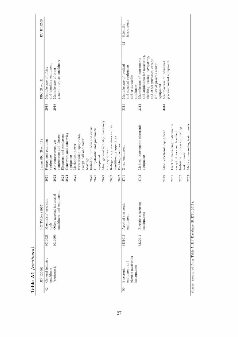
AIndustryconcordance

TableA1:Industryconcordanceamonginternationaldatabases.

JIP(2006)

I-OTables(1995)

JapanSIC

(Rev.11)

ISIC

(Rev.3)

EUKLEMS

51Semiconductor

3341011

Semiconductordevices

2912

Semiconductordevices

3210

Manufactureofelectronic

29Electronicvalves

devicesand

valvesandtubesandother

andtubes

integratedcircuits

electroniccomponents

3341012

Integratedcircuits

2913

Integratedcircuits

52Electronicparts

3359011

Electrontubes

2793

Magnetictapesanddiscs

3210

Manufactureofelectronic

29Electronicvalves

valvesandtubesandother

andtubes

electroniccomponents

3359021

Liquidcrystaldevices

2911

Electrontubes

3230

ManufactureofTVand

31RadioandTV

radioreceivers,soundor

receivers

videorecordingor

reproducingapparatus,

andassociatedgoods

3359031

Magnetictapesanddiscs

2914

Resistors,capacitors,

transformersand

compositeparts

3359099

Otherelectronic

2915

Electroacoustictransducers,

components

magneticheads,andsmallmotors

2916

Connectors,switchesandrelays

2917

Switchingpowersupplies

2918

Printedcircuit

2919

Misc.parts

42Generalindustry

3011011

Boilers

2611

Boilers

2813

Manufactureofsteam

24Fabricated

machinery

generators,exceptcentral

metalproducts

heatinghotwaterboilers

3011021

Turbines

2612

Steam

engines,turbinesand

2893

Manufactureofcutlery,

25Machinery,NEC

waterwheels,exceptmarine

handtoolsandgeneral

engines

hardware

3011031

Engines

2613

Internalcombustionengines

2911

Manufactureofengines

andturbinesexceptaircraft,

vehicleandcycleengines

3012011

Conveyors

2619

Misc.enginesandturbines

2912

Manufactureofpumps,

compressors,tapsandvalves

3013011

Refrigeratorsandair

2644

Machinists�precisiontools

2913

Manufactureofbearings,

conditioningapparatus

exceptpowdermetallurgy

gears,gearinganddriving

products

elements

3019011

Pumpsandcompressors

2668

Vacuumequipmentand

2914

Manufactureofovens,

vacuumcomponent

furnacesandfurnaceburners

manufacture

26

TableA1(continued)

JIP(2006)

I-OTables(1995)

JapanSIC

(Rev.11)

ISIC

(Rev.3)

EUKLEMS

42Generalindustry

3019021

Machinists�precision

2671

Pumpsandpumping

2915

Manufactureoflifting

machinery

tools

equipment

andhandlingequipment

(continued)

3019099

Othergeneralindustrial

2672

Aircompressors,gas

2919

Manufactureofother

machineryandequipment

compressorsandblowers

generalpurposemachinery

2673

Elevatorsandescalators

2674

Conveyorsandconveying

equipment

2675

Mechanicalpower

transmissionequipment,

exceptballandroller

bearings

2676

Industrialfurnacesandovens

2677

Oilhydraulicandpneumatic

equipment

2679

Misc.generalindustrymachinery

andequipment

2682

Refrigeratingmachinesandair

conditioningapparatus

2697

Packingmachines

50Electronic

3331011

Appliedelectronic

2741

X-rayequipment

3311

Manufactureofmedical

32Scienti�c

equipmentand

equipment

andsurgicalequipment

instruments

electricmeasuring

andorthopaedic

instruments

appliances

3332011

Electricmeasuring

2743

Medicalinstrumentselectronic

3312

Manufactureofinstruments

instruments

equipment

andappliancesformeasuring,

checking,testing,navigating,

andotherpurposes,except

industrialprocesscontrol

equipment

2749

Misc.electronicequipment

3313

Manufactureofindustrial

processcontrolequipment

2751

Electricmeasuringinstruments

exceptotherwiseclassi�ed

2752

Industrialprocesscontrolling

instruments

2753

Medicalmeasuringinstruments

Source:excerptedfrom

Table7,JIPDatabase(RIETI,2011).

27

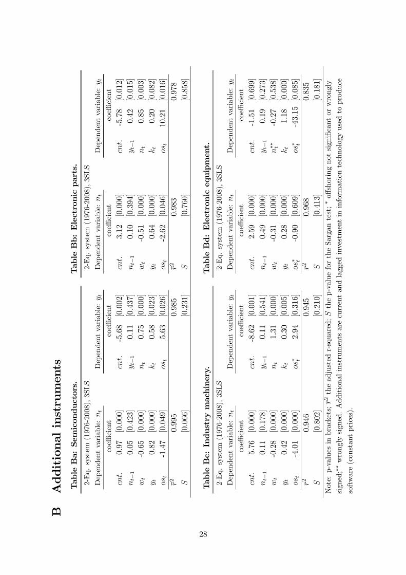
BAdditionalinstruments

TableBa:Semiconductors.

2-Eq.system

(1976-2008),3SLS



coe¢cient

coe¢cient

cnt:

0.97

[0:000]

cnt:

-5.68[0:002]

nt�1

0.05

[0:423]

y t�1

0.11

[0:437]

wt

-0.65[0:000]

nt

0.75

[0:000]

y t0.82

[0:000]

kt

0.58

[0:023]

ost

-1.47[0:049]

ost

5.63

[0:026]

r20.995

0.985

S[0:066]

[0:231]

TableBb:Electronicparts.

2-Eq.system

(1976-2008),3SLS



coe¢cient

coe¢cient

cnt:

3.12

[0:000]

cnt:

-5.78[0:012]

nt�1

0.10

[0:394]

y t�1

0.42

[0:015]

wt

-0.51[0:000]

nt

0.85

[0:003]

y t0.64

[0:000]

kt

0.20

[0:082]

ost

-2.62[0:046]

ost

10.21[0:016]

r20.983

0.978

S[0:760]

[0:858]

TableBc:Industrymachinery.

2-Eq.system

(1976-2008),3SLS



coe¢cient

coe¢cient

cnt:

5.76

[0:000]

cnt:

-8.62[0:001]

nt�1

0.11

[0:178]

y t�1

0.11

[0:541]

wt

-0.28[0:000]

nt

1.31

[0:000]

y t0.42

[0:000]

kt

0.30

[0:005]

ost

-4.01[0:000]

os� t

2.94

[0:316]

r20.946

0.945

S[0:802]

[0:210]

TableBd:Electronicequipment.

2-Eq.system

(1976-2008),3SLS



coe¢cient

coe¢cient

cnt:

2.59

[0:000]

cnt:

-1.51[0:699]

nt�1

0.49

[0:000]

y t�1

0.19

[0:273]

wt

-0.31[0:000]

n�� t

-0.27[0:538]

y t0.28

[0:000]

kt

1.18

[0:000]

os� t

-0.90[0:609]

os� t

-43.15

[0:085]

r20.968

0.835

S[0:413]

[0:181]

Note:p-valuesinbrackets;r2theadjustedr-squared;Sthep-valuefortheSargantest;�o¤shoringnotsigni�cantorwrongly

signed;��wronglysigned.Additionalinstrumentsarecurrentandlaggedinvestmentininformationtechnologyusedtoproduce

software(constantprices).

28

offshoring and productivity revisited: a time-series analysisftp.iza.org/dp7323.pdf · offshoring...

Documents