Fast randomized iteration: diffusion Monte Carlo through the lens

of numerical linear algebra

Lek-Heng Lim1 and Jonathan Weare1,2

1Department of Statistics, University of Chicago2James Franck Institute, University of Chicago

Abstract

We review the basic outline of the highly successful diffusion Monte Carlo technique com-monly used in contexts ranging from electronic structure calculations to rare event simulationand data assimilation, and propose a new class of randomized iterative algorithms based on sim-ilar principles to address a variety of common tasks in numerical linear algebra. From the pointof view of numerical linear algebra, the main novelty of the Fast Randomized Iteration schemesdescribed in this article is that they work in either linear or constant cost per iteration (andin total, under appropriate conditions) and are rather versatile: we will show how they applyto solution of linear systems, eigenvalue problems, and matrix exponentiation, in dimensionsfar beyond the present limits of numerical linear algebra. While traditional iterative methodsin numerical linear algebra were created in part to deal with instances where a matrix (of sizeO(n2)) is too big to store, the algorithms that we propose are effective even in instances wherethe solution vector itself (of size O(n)) may be too big to store or manipulate. In fact, our workis motivated by recent DMC based quantum Monte Carlo schemes that have been applied tomatrices as large as 10108×10108. We provide basic convergence results, discuss the dependenceof these results on the dimension of the system, and demonstrate dramatic cost savings on arange of test problems.

1 Introduction

Numerical linear algebra has been the cornerstone of scientific computing from its earliest daysand randomized approaches to solving problems in linear algebra have a history almost as long asnumerical linear algebra itself (see e.g. [1, 18, 19, 25, 34, 35, 36, 37, 38, 62]).1 As the size of matricesencountered in typical applications has increased (e.g. as we sought greater and greater accuracy innumerical solution of partial differential equations), so has the attention paid to the performance oflinear algebra routines on very large matrices both in terms of memory usage and operations count.Today, in applications ranging from numerical solution of partial differential equations (PDE) todata analysis, we are frequently faced with the need to solve linear algebraic problems at andbeyond the boundary of applicability of classical techniques. In response, randomized numericallinear algebra algorithms are receiving renewed attention and, over the last decade, have becomean immensely popular subject of study within the applied mathematics and computer sciencecommunities (see e.g. [14, 20, 21, 22, 24, 28, 44, 46, 54, 55, 61, 64]).

The goal of this article is to, after providing a brief introduction to the highly successful diffusionMonte Carlo (DMC) algorithm, suggest a new class of algorithms inspired by DMC for problems in

1As pointed out in [30] many classical iterative techniques in numerical linear algebra are intimately related toMarkov chain Monte Carlo (MCMC) schemes.

1

arX

iv:1

508.

0610

4v3

[m

ath.

NA

] 9

Oct

201

7

numerical linear algebra. DMC is used in applications including electronic structure calculations,rare event simulation, and data assimilation, to efficiently approximate expectations of the typeappearing in Feynman–Kac formulae, i.e., for weighted expectations of Markov processes typicallyassociated with parabolic partial differential equations (see e.g. [16]). While based on principlesunderlying DMC, the Fast Randomized Iteration (FRI) schemes that we study in this article aredesigned to address arguably the most classical and common tasks in matrix computations: linearsystems, eigenvector problems, and matrix exponentiation, i.e., solving for v in

Av = b, Av = λv, v = exp(A)b (1)

for matrices A that might not have any natural association with a Markov process.FRI schemes rely on basic principles similar to those at the core of other randomized methods

that have appeared recently in the numerical linear algebra literature but they differ substantiallyin detail and in the problems they address. These differences will be remarked on again later,but roughly, while many recent randomized linear algebra techniques rely on a single samplingstep, FRI methods randomize repeatedly and, as a consequence, are more sensitive to errors inthe constructed randomizations. FRI schemes are not, however, the first to employ randomizationwithin iterative schemes (see in particular [1] and [34]). In fact the strategy of replacing expensiveintegrals or sums (without immediate stochastic interpretation) appearing in iterative protocols hasa long history in a diverse array of fields. For example, it was used in schemes for the numericalsolution of hyperbolic systems of partial differential equations in [11]. That strategy is representedtoday in applications ranging from density functional calculations in physics and chemistry (seee.g. [3]) to maximum likelihood estimation in statistics and machine learning (see e.g. [8]). Thoughrelated in that they rely on repeated randomization within an iterative procedure, these schemesdiffer from the methods we consider in that they do not use a stochastic representation of thesolution vector itself. In contrast to these and other randomized methods that have been usedin linear algebra applications, our focus is on problems for which the solution vector is extremelylarge so they can only be treated by linear or constant cost algorithms. In fact, the scheme that isour primary focus is ideally suited to problems so large that the solution vector itself is too largeto store so that no traditional iterative method (even for sparse matrices) is appropriate. This ispossible because our scheme computes only low dimensional projections of the solution vector andnot the solution vector itself. The full solution is replaced by a sequence of sparse random vectorswhose expectations are close to the true solution and whose variances are small.

Diffusion Monte Carlo (see e.g. [2, 7, 10, 26, 32, 33, 40, 42, 45]) is a central component in thequantum Monte Carlo (QMC) approach to computing the electronic ground state energy of theSchrodinger–Hamiltonian operator2

Hv = −1

2∆v + U v. (2)

We are motivated in particular by the work in [7] in which the authors apply a version of the DMCprocedure to a finite (but huge) dimensional projection of H onto a discrete basis respecting ananti-symmetry property of the desired eigenfunction. The approach in [7] and subsequent papershave yielded remarkable results in situations where the projected Hamiltonian is an extremely largematrix (e.g. 10108 × 10108, see [59]) and standard approaches to finite dimensional eigenproblemsare far from reasonable (see [4, 5, 6, 12, 13, 59]).

The basic DMC approach is also at the core of schemes developed for a number of applicationsbeyond electronic structure. In fact, early incarnations of DMC were used in the simulation of small

2The symbol ∆ is used here and below to denote the usual Laplacian operator on functions of Rd, ∆u =∑di=1 ∂

2xiu.

U is a potential function that acts on v by pointwise multiplication. Though this operator is symmetric, the FRIschemes we introduce below are not restricted to symmetric eigenproblems.

2

probability events [39, 56] for statistical physics models. Also in statistical physics, the transfermatrix Monte Carlo (TMMC) method was developed to compute the partition functions of certainlattice models by exploiting the observation that the partition function can be represented as thedominant eigenvalue of the so-called transfer matrix, a real, positive, and sparse matrix (see [48]).TMMC may be regarded as an application of DMC to discrete eigenproblems. DMC has alsobecome a popular method for many data assimilation problems and the notion of a “compression”operation introduced below is very closely related to the “resampling” strategies developed for thoseproblems (see e.g. [31, 41, 15]).

One can view the basic DMC (or MCMC for that matter) procedure as a combination of twosteps: In one step an integral operator (a Green’s function) is applied to an approximate solutionconsisting of a weighted finite sum of delta functions, in another step the resulting function (whichis no longer a finite mixture of delta functions) is again approximated by a finite mixture of deltafunctions. The more delta functions allowed in the mixture, the higher the accuracy and cost ofthe method. A key to understanding the success of these methods is the observation that not alldelta functions (i.e., at all positions in space) need appear in the mixture. A similar observationholds for the methods we introduce: FRI schemes need not access all entries in the matrix ofinterest to yield an accurate solution. In fact, we prove that the cost to achieve a fixed level ofaccuracy with our methods can be bounded independently of the size of the matrix, though inmany applications one should expect some dependence on dimension. As with other randomizedschemes, when an effective deterministic method is available it will very likely outperform themethods we propose; our focus is on problems for which satisfactory deterministic alternatives arenot available (e.g. when the size of the intermediate iterates or final result are so large as to prohibitany conceivable deterministic methods). Moreover, the schemes that we propose are a supplementand not a replacement for traditional dimensional reduction strategies (e.g. intelligent choice ofbasis). Indeed, successful application of DMC within practical QMC applications relies heavily ona change of variables based on approximations extracted by other methods (see the discussion ofimportance sampling in [26]).

The theoretical results that we provide are somewhat atypical of results commonly presentedin the numerical linear algebra literature. In the context of linear algebra applications, both DMCand FRI schemes are most naturally viewed as randomizations of standard iterative procedures andtheir performance is largely determined by the structure of the particular deterministic iterationbeing randomized. For this reason, as well as to avoid obscuring the essential issues with the detailsof individual cases, we choose to frame our results in terms of the difference between the iterates vtproduced by a general iterative scheme and the iterates generated by the corresponding randomizedscheme Vt (rather than considering the difference between Vt and limt→∞ vt). In ideal situations(see Corollary 1) our bounds are of the form

|||Vt − vt||| := supf∈Cn, ‖f‖∞≤1

√E [|f · Vt − f · vt|2] ≤ C√

m(3)

where the (in general t-dependent) constant C is independent of the dimension n of the problem andm ≤ n controls the cost per iteration of the randomized scheme (one iteration of the randomizedscheme is roughly a factor of n/m less costly than its deterministic counterpart and the two schemesare identical when m = n). The norm in (3) measures the root mean squared deviation in lowdimensional projections of the iterates. This choice is important as described in more detail inSections 3 and 4. For more general applications, one can expect the constant C, which incorporatesthe stability properties of the randomized iteration, to depend on dimension. In the worst casescenario, the randomized scheme is no more efficient than its deterministic counterpart (in otherwords, reasonable performance may require m ∼ n). Our numerical simulations, in which n/mranges roughly between 107 and 1014, strongly suggest that this scenario may be rare.

3

We will begin our development in Section 2 with a description of the basic diffusion MonteCarlo procedure. Next, in Section 3 we describe how ideas borrowed from DMC can be applied togeneral iterative procedures in numerical linear algebra. As a prototypical example, we describehow randomization can be used to dramatically decrease the cost of finding the dominant eigen-value and (projections of) the dominant eigenvector. Also in that section, we consider the specificcase in which the iteration mapping is an ε-perturbation of the identity, relevant to a wide rangeof applications involving evolutionary differential equations. In this case a poorly chosen random-ization scheme can result in an unstable algorithm while a well chosen randomization can result inan error that decreases with ε (over ε−1 iterations). Next, in Sections 4 and 5, we establish severalsimple bounds regarding the stability and error of our schemes. Finally, in Section 6 we providethree computational examples to demonstrate the performance of our approach. A simple, educa-tional implementation of Fast Randomized Iteration applied to our first computational example isavailable online (see [63]).

Remark 1. In several places we have included remarks that clarify or emphasize concepts that mayotherwise be unclear to readers more familiar with classical, deterministic, numerical linear algebramethods. We anticipate that some of these remarks will be useful to this article’s broader audienceas well.

2 Diffusion Monte Carlo within quantum Monte Carlo

The ground state energy, λ∗, of a quantum mechanical system governed by the Hamiltonian in (2)is the smallest eigenvalue (with corresponding eigenfunction v∗) of the Hermitian operator H. Thestarting point for a DMC calculation is the imaginary-time Schrodinger equation34

∂tv = −Hv (4)(for a review of QMC see [26]). One can, in principle, use power iteration to find λ∗: beginningfrom an initial guess v0 (and assuming a gap between λ∗ and the rest of the spectrum of H), theiteration

λt = −1

εlog

∫e−εHvt−1(x) dx and vt =

e−εHvt−1∫e−εHvt−1(x) dx

(5)

will converge to the pair (λ∗, v∗) where v∗ is the eigenfunction corresponding to λ∗. Here the integralis over x ∈ Rd.Remark 2. For readers who are more familiar with the power method in numerical linear algebra,this may seem a bit odd but a discrete analogue of (5) is just vt = Avt−1/‖Avt−1‖1 applied toa positive definite matrix A = exp(−εH) ∈ Cn×n where H is Hermitian.5 The slight departurefrom the usual power method is only in (i) normalizing by a 1-norm (or rather, by the sum ofentries 1TAvt−1 since both v and A are non-negative), and (ii) iterating on exp(−εH) instead ofon H directly (the goal in this context is to find the smallest eigenvalue of H not the magnitude-dominant eigenvalue of H). The iteration on the eigenvalue is then λt = −ε−1 log‖Avt−1‖1 sinceλ∗(H) = −ε−1 log λ∗(A).

3The reader familiar with quantum mechanics but unfamiliar with QMC may wonder why we begin with theimaginary time Schrodinger equation and not the usual Schrodinger equation i∂tv = −Hv. The reason is that whilethe solutions to both equations can be expanded in terms of the eigenfunctions of H, for the usual Schrodingerequation the contributions to the solution from eigenfunctions with larger eigenvalues do not decay relative to theground state. By approximating the solution to the imaginary time equation for large times we can approximate theground state eigenfunction of H.

4 In practical QMC applications one solves for ρ = v∗v where v is an approximate solution found in advanceby other methods. The new function ρ is the ground state eigenfunction of a Hamiltonian of the form Hv =− 1

2∆v + div(bv) + Uv. The implications for the discussion in this section are minor.5Note that the matrix H is not the same as the operator H on a function space, and is only introduced for the

purposes of relating the expression in (5) to the usual power method for matrices

4

The first step in any (deterministic or stochastic) practical implementation of (5) is discretiza-tion of the operator e−εH. Diffusion Monte Carlo often uses the second order time discretization

e−εH ≈ Kε = e−ε2Ue

ε2

∆e−ε2U .

A standard deterministic approach would then proceed by discretizing the operator Kε in space andreplacing e−εH in (5) with the space and time discretized approximate operator. The number ofspatial discretization points required by such a scheme to achieve a fixed accuracy will, in general,grow exponentially in the dimension d of x.

Diffusion Monte Carlo uses two randomization steps to avoid this explosion in cost as d increases.These randomizations have the effect of ensuring that the random approximations V m

t of the iteratesvt are always of the form

V mt (x) =

∑Nt

j=1W

(j)t δ

X(j)t

(x)

where δy(x) is the Dirac delta function centered at y ∈ Rd, the W(j)t are real, non-negative numbers

with E[∑Nt

j=1W(j)t

]= 1, and, for each j ≤ Nt, X

(j)t ∈ Rd. As will be made clear in a moment, the

integer m superscripted in our notation controls the number of delta functions, Nt, included in theabove expression for V m

t .The fact that the function V m

t is non-zero at only Nt values is crucial to the efficiency of diffusionMonte Carlo. Starting with N0 = m and from an initial condition of the form

V m0 =

1

m

∑m

j=1δX

(j)0

the first factor of e−ε2U applied to V m

0 results in

1

m

∑m

j=1e−

ε2U(X

(j)0 )δ

X(j)0

which can be assembled in O(m) operations. The first of the randomization steps used in DMCrelies on the well known relationship∫

f(x)[eε2

∆δy](x) dx = Ey [f(Bε)] (6)

where f is a test function, Bs is a standard Brownian motion evaluated at time s ≥ 0, and thesubscript on the expectation is meant to indicate that B0 = y (i.e., in the expectation in (6) Bε isa Gaussian random variable with mean y and variance ε). In fact, this representation is a specialcase of the Feynman–Kac formula

∫f(x)[e−εHδy](x) dx = Ey

[f(Bε)e

−∫ ε0 U(Bs) ds

]. Representation

(6) suggests the approximation

KεVm

0 ≈ V m1 =

1

m

∑m

j=1e−

ε2

(U(ξ

(j)1 )+U(X

(j)0 ))δξ(j)1

where, conditioned on the X(j)0 , the ξ

(j)1 are independent and ξ

(j)1 is normally distributed with mean

X(j)0 and covariance εI (here I is the d× d identity matrix). This first randomization has allowed

an approximation of KεVm

0 by a distribution, V m1 , that is again supported on only m points in Rd.

One might, therefore, attempt to define a sequence V mt iteratively by the recursion

V mt+1 =

V mt+1∫

V mt+1(x) dx

=∑m

j=1W

(j)t+1 δξ(j)t+1

where we have recursively defined the weights

W(j)t+1 =

e−ε2

(U(ξ

(j)t+1)+U(X

(j)t ))W

(j)t∑m

`=1 e− ε

2

(U(ξ

(`)t+1)+U(X

(`)t ))W

(`)t

5

with W(j)0 = 1/m for each j. The cost of this randomization procedure is O(dm) so that the total

cost of a single iteration is O(dm).At each step the weights in the expression for the iterates V m

t are multiplied by additional

random factors. These factors are determined by the potential U and the positions of the ξ(j)t . On

the other hand, the ξ(j)t , evolve without reference to the potential function U (they are discretely

sampled points from m independent Brownian motions). As a consequence, over many iterations

one can expect extreme relative variations in the W(j)t and, therefore, poor accuracy in V m

t as anapproximation of the functions vt produced by (5).

The second randomization employed by the DMC algorithm is the key to controlling the growthin variance and generalizations of the idea will be key to designing fast randomized iteration schemesin the next section. In order to control the variation in weights, at step t, DMC randomly re-

moves points ξ(j)t corresponding to small weights W

(j)t and duplicates points corresponding to large

weights. The resulting number of points stored at each iteration, Nt, is close to, or exactly, m. Atstep t, a new distribution Y m

t is generated from V mt so that

E [Y mt | V m

t ] = V mt

by “resampling” a new collection of Nt+1 points from the Nt points ξ(j)t with associated probabilities

W(j)t . The resulting points are labeled X

(j)t and the new distribution Y m

t takes the form

Y mt =

1

Nt

∑Nt+1

j=1δX

(j)t.

The next iterate V mt+1 is then built exactly as before but with V m

t replaced by Y mt . All methods to

select the X(j)t generate, for each j, a non-negative integer N

(j)t with

E[N

(j)t

∣∣ {W (`)t

}m`=1

]= mW

(j)t

and then sets N(j)t of the elements in the collection {X(j)

t }Nt+1

j=1 equal to ξ(j)t so that Nt+1 =∑Nt

j=1N(j)t . For example, one popular strategy in DMC generates the N

(j)t independently with

P[N

(j)t =

⌊mW

(j)t

⌋]=⌈mW

(j)t

⌉−mW (j)

t ,

P[N

(j)t =

⌈mW

(j)t

⌉]= mW

(j)t −

⌊mW

(j)t

⌋.

(7)

The above steps define a randomized iterative algorithm to generate approximations V mt of

vt. The second randomization procedure (generating Y mt from V m

t ) will typically require O(m)operations, preserving the overall O(dm) per iteration cost of DMC (as we have described it). Thememory requirements of the scheme are also O(dm). The eigenvalue λ∗ can be approximated, forexample, by

−1

εlog

(1

T

∑T

t=1

1

Nt

∑Nt

j=1e− ε

2

(U(ξ

(j)t+1)+U(X

(j)t )

))for T large.

Before moving on to more general problems notice that the scheme just outlined applies just aseasily to space-time discretizations of e−εH. For example, if we set h =

√(1 + 2d)ε and denote by

Edh ⊂ Rd the uniform rectangular grid with resolution h in each direction, the operator e−εH canbe discretized using

e−εH ≈ Kε,h = e−ε2Ue

ε2

∆he−ε2U

where, for any vector g ∈ Edh ,

∆hg(x) =1

ε

(−g(x) +

1

1 + 2d

∑y∈Edh, ‖y−x‖2≤h

g(y)

)

6

(here we find it convenient to identify functions g : Edh → R and vectors in REdh). The operatore−ε∆h again has a stochastic representation; now the representation is in terms of a jump Markovprocess with jumps from a point in Edh to one of its nearest neighbors on the grid (for an interestingapproach to discretizing stochastic differential equations taking advantage of a similar observationsee [9]).

Remark 3. The reader should notice that not only will we be unable to store the matrix Kε,h

(which is exponentially large in d) or afford to compute Kε,hv for a general vector v, but we willnot even be able to store the iterates vt generated by the power method. Even the sparse matrixroutines developed in numerical linear algebra to deal with large matrices are not reasonable forthis problem.

In this discrete context, a direct application of the DMC approach (as in [48]) would representthe solution vector as a superposition of standard basis elements6 and replace calculation of Kε,hvby a random approximation whose cost is (for this particular problem) free of any direct dependenceon the size of Kε,h (though its cost can depend on structural properties of Kε,h which may be relatedto its size), whose expectation is exactly Kε,hv, and whose variance is small. The approach in [7]is also an application of these same basic DMC steps to a discrete problem, though in that casethe desired eigenvector has entries of a priori unkown sign, requiring that the solution vector berepresented by a superposition of signed standard basis elements.

In this article we take a different approach to adapting DMC to discrete problems. Instead ofreproducing in the discrete setting exactly the steps comprising DMC, consider a slightly modifiedscheme that omits direct randomization of an approximation to eε∆h , and instead relies solely ona general random mapping Φm

t very similar to the map from V mt to Y m

t but which takes a vector

V mt ∈ REdh with non-negative entries and ‖V m

t ‖1 = 1 (i.e., a probability measure on {1, 2, . . . , |Edh |})and produces a new random vector Y m

t with m, or nearly m, non-zero components and satisfyingE [Y m

t | V mt ] = V m

t as above. Starting from a non-negative initial vector V m0 ∈ Edh with ‖V m

0 ‖1 = 1and with at most O(md) non-zero entries, V m

t+1 is generated from V mt as follows:

Step 1. Generate Y mt = Φm

t (V mt ) with approximately or exactly m non-zero entries.

Step 2. Set V mt+1 =

Kε,hYmt

‖Kε,hYmt ‖1

.

Just as at iteration t, DMC produces a random approximation of the result of t iterations of poweriteration for the infinite dimensional integral operator e−εH, the above steps produce a randomapproximation of the result of t iterations of the power iteration for the matrix Kε,h. The improvedefficiency of DMC is due to the application of the integral operator to a finite sum of delta functionsin place of a more general function. Similarly, the efficiency of the finite dimensional method inthe above two step procedure is a consequence of replacement of a general vector v in the productKε,hv by a sparse approximation, Φm

t (v).For the random mapping Φm

t (v) we might, for example, adapt the popular resampling choicementioned above and choose the entries of Y m

t independently with

P[(Y mt )j =

⌊(V mt )jm

⌋/m]

=⌈(V mt )jm

⌉− (V m

t )jm,

P[(Y mt )j =

⌈(V mt )jm

⌉/m]

= (V mt )jm−

⌊(V mt )jm

⌋.

(8)

Note that this rule results in a vector Y mt with expectation exactly equal to V m

t . On the otherhand, when the number of non-zero entries in V m

t is large, many of those entries must be less than

6The delta functions represent the indices of vt that we are keeping track of; δξ is more commonly denoted eξ innumerical linear algebra — the standard basis vector with 1 in the ξth coordinate and zero elsewhere.

7

1/m (because ‖V mt ‖1 = 1) and will have some probability of being set equal to zero in Y m

t . In fact,the number of non-zero entries in Y m

t has expectation and variance bounded by m. The details ofthe mappings Φm

t , which we call compression mappings, will be described later in Section 5 where,for example, we will find that the cost of applying the mapping Φm

t will typically be O(n) whenits argument has n non-zero entries (in this setting n = O(md)). And while the cost of applying

Kε,h to an arbitrary vector in REdh is |Edh |, the cost of applying Kε,h to a vector with m non-zeroentries is only O(md). The total cost of the scheme per iteration is therefore O(md) in storageand operations. These cost requirements are dependent on the particular spatial discretization ofeε∆; if we had chosen a discretization corresponding to a dense matrix Kε,h then the cost reductionwould be much less extreme. Nonetheless, as we will see in Section 3, the scheme just describedcan be easily generalized and, as we will see in Sections 4 and 6, will often result in methods thatare significantly faster than their deterministic counterparts.

Remark 4. Rather than focusing on sampling indices of entries in a vector v, as is typical of someof the literature on randomized numerical linear algebra, we focus on constructing an accuratesparse representation of v. This is primarily a difference of perspective, but has consequences forthe accuracy of our randomizations. For example, the techniques in [18, 19] and in [20, 21, 22]would correspond, in our notation and context, to setting for v ∈ Rn

Φmt (v) =

‖v‖1m

n∑j=1

vj|vj |

N(j)t ej (9)

where ej is the jth standard basis element and the random vector(N

(1)t , N

(2)t , . . . , N

(n)t

)∼Multinomial(m, p1, . . . , pn)

with pj = |vj |/‖v‖1. As for all Monte Carlo methods, the sparse characteristic of this representationis responsible for gains in efficiency. And, when error is measured by the norm in (3), only a randomsparse representation can be accurate for general v. But random index selection yields only one ofmany possible random sparse representations of v and not one that is particularly accurate. In fact,effective fast randomized iteration schemes of the type introduced in this paper cannot be based solelyon random index selection as in (9). In the setting of this section, if we were to use (9) in place ofthe rule in (8) the result would be an unstable scheme (the error would become uncontrollable as εis decreased). As we will see in Section 5, much more accurate sparse representations are possible.

Even restricting ourselves to the quantum Monte Carlo context, there is ample motivation togeneralize the DMC scheme. Often one wishes to approximate not the smallest eigenvalue of Hbut instead the smallest eigenvalue corresponding to an antisymmetric (in exchange of particlepositions) eigenfunction. DMC as described in this section, cannot be applied directly to com-puting this value, a difficulty commonly referred to as the Fermion sign problem. Several authorshave attempted to address this issue with various modifications of DMC. In particular, Alavi andcoworkers recently developed a version of DMC for a particular spatial disretization of the Hamilto-nian (in the configuration interaction basis) that exactly preserves antisymmetry (unlike the finitedifference discretization we just described). Run to convergence, their method provides the sameapproximation as the so called full CI method but can be applied with a much larger basis (e.g. inexperiments by Alavi and coworkers reported in [59] up to 10108 total functions in the expansionof the solution). Though the generalizations of DMC represented by the two step procedure in thelast paragraph and by the developments in the next section are motivated by the scheme proposedin [7], they differ substantially in their details and can be applied to a wider range of problems(including different discretizations of H). Finally we remark that, while we have considered DMCin the particular context of computing the ground state energy of a Hamiltonian, the method isused for a much wider variety of tasks with only minor modification to its basic structure. For

8

example, particle filters (see e.g. [15]) are an application DMC to on-line data assimilation andsubstantive differences are mostly in the interpretation of the operator to which DMC is applied(and the fact that one is typically interested in the solution after finitely many iterations).

3 A general framework

Consider the general iterative procedure,

vt+1 =M(vt) (10)

for vt ∈ Cn. Eigenproblems, linear systems, and matrix exponentiation can each be accomplishedby versions of this iteration. In each of those settings the cost of evaluatingM(v) is dominated bya matrix-vector multiplication. We assume that the cost (in terms of floating point operations andstorage) of performing the required matrix-vector multiplication makes it impossible to carry outrecursion (10) to the desired precision. As in the steps described at the end of the last section, wewill consider the error resulting from replacement of (10) by

V mt+1 =M (Φm

t (V mt )) . (11)

where the compression maps Φmt : Cn → Cn are independent, inexpensive to evaluate, and enforce

sparsity in the V mt iterates (the number of non-zero entries in V m

t will be O(m)) so that M canbe evaluated at much less expense. When M is a perturbation of identity and an O(n) scheme isappropriate (see Sections 3.2 and 4 below) we will also consider the scheme,

V mt+1 = V m

t +M (Φmt (V m

t ))− Φmt (V m

t ). (12)

The compressions Φmt will satisfy (or very nearly satisfy) the statistical consistency criterion

E [Φmt (v)] = v

and will have to be carefully constructed to avoid instabilities and yield effective methods. Fordefiniteness one can imagine that Φm

t is defined by a natural extension of (8)

P

[(Φm

t (v))j =vj

m|vj |

⌊m|vj |‖v‖1

⌋]=

⌈m|vj |‖v‖1

⌉− m|vj |‖v‖1

,

P

[(Φm

t (v))j =vj

m|vj |

⌈m|vj |‖v‖1

⌉]=m|vj |‖v‖1

−⌊m|vj |‖v‖1

⌋ (13)

to accept arguments v ∈ Cn (V mt is no longer a non-negative real number). This choice has several

drawbacks, not least of which is its cost, and we do not use it in our numerical experiments. Alter-native compression schemes, including the one used in our numerical simulations, are considered indetail in Section 5. There we will learn that one can expect that, for any pair f, v ∈ Cn,√

E [|fHΦmt (v)− fHv|2] ≤ 2√

m‖f‖∞‖v‖1 (14)

(the superscript H is used throughout this article to denote the conjugate transpose of a vector withcomplex entries). These errors are introduced at each iteration and need to be removed to obtainan accurate estimate. Depending on the setting, we may rely on averaging over long trajectories,averaging over parallel simulations (replicas), or dynamical self-averaging (see Sections 3.2 and 4),to remove the noise introduced by our randomization procedure. Because the specific choice of Mand the form of averaging used to remove noise can differ substantially by setting, we will describethe schemes within the context of specific (and common) iterative procedures.

3.1. The eigenproblem revisited Consider, for example, a more general eigenproblem than theone we considered in Section 2. Given K ∈ Cn×n the goal is to determine λ∗ ∈ C and v∗ ∈ Cn suchthat

Kv∗ = λ∗v∗ (15)

9

and such that, for any other solution pair (λ, v), |λ| < |λ∗|. In what follows in this section we willassume that this problem has a unique solution. The standard methods of approximate solution of(15) are variants of the power method, a simple version of which performs

vt+1 =Kvt‖Kvt‖1

, λt+1 =uHKvtuHvt

(16)

where u ∈ Cn is chosen by the user. Under generic conditions, these converge to the correct (λ∗, v∗)starting from an appropriate initial vector v0 (see e.g. [17]). The scheme in (16) requires O(n2)work per iteration and at least O (n) storage. In this article, we are interested in situations inwhich these cost and storage requirements are unreasonable.

From O(n2)to O (nm) For the iteration in (16) the randomized scheme (11) (along with an

approximation of λ∗) becomes

V mt+1 =

KΦmt (V m

t )

‖KΦmt (V m

t )‖1, Λmt+1 =

uHKΦmt (V m

t )

uHV mt

,

Vmt =

1

t

t∑s=1

V ms , Λ

mt , =

1

t

t∑s=1

Λmt

(17)

where Vmt and Λ

mt are trajectory averages estimating v∗ and λ∗. In (17), the compressions Φm

t areindependent of one another. Using the rules defining Φm

t in Section 5, construction of Φmt (V m

t )at each step will require O(n) operations. Since multiplication of the vector Φm

t (V mt ) by a dense

matrix K requires O(nm) operations, this scheme has O(nm) cost and O(n) storage per iterationrequirement.

Iteration (12) on the other hand replaces (16) with

V mt+1 = V m

t +

(KΦm

t (V mt )

‖KΦmt (V m

t )‖1− Φm

t (V mt )

), Λmt+1 =

uHKΦmt (V m

t )

uHV mt

. (18)

By the same arguments as above, this iteration will also have cost and storage requirements ofO(nm) and O(n) respectively. When K = I + εA for some matrix A and small parameter ε > 0,the iteration in (18) bears strong resemblance to the Robbins–Monro stochastic approximationalgorithm [53, 43]. In fact, as we will see in Section 4, when the mappingM is of the form v+εb(v)the convergence of methods of the form in (11) and (12) is reliant on the self-averaging phenomenonalso at the heart of stochastic approximation. We will also learn that for M of this form one canexpect the error corresponding to (12) to be smaller than the error corresponding to (11).

From O(nm) to O(m) For many problems even O(nm) cost and storage requirements are un-acceptable. This is the case, for example, when n is so large that a vector of length n cannot bestored. But now suppose that K is sparse with at most q non-zero entries per column. BecauseΦmt−1(V m

t−1) has O(m) non-zero entries, the product KΦmt−1(V m

t−1) (and hence also V mt ) has at most

O(qm) entries and requires O(qm) operations to assemble. On the other hand, if V mt has at most

O(qm) non-zero entries, then application of Φmt to V m

t requires only O(qm) operations. Conse-quently, as long as V m

0 has at most O(qm) non-zero entries, the total number of floating pointoperations required by (17) reduces to O (qm) per iteration. This observation does not hold formethods of the form (12) which will typically result in dense iterates V m

t and a cost of O(n) evenwhen K is sparse.

As we have mentioned (and as was true in Section 2), in many settings even storing the fullsolution vector is impossible. Overcoming this impediment requires a departure from the usualperspective of numerical linear algebra. Instead of trying to approximate all entries of v∗, our goalbecomes to compute

f∗ = fHv∗

10

for some some vector (or small number of vectors) f. This change in perspective is reflected inthe form of our compression rule error estimate in (14) and in the form of our convergence resultsin Section 4 that measure error in terms of dot products with test vectors as in (3) above. Asdiscussed in more detail in Section 4, the choice of error norm in (3) is essential to our eventualerror estimates. Indeed, were we to estimate a more standard quantity such as

E [‖V mt − vt‖1]

we would find that the error decreased proportional to (n−m)/n requiring that m increase with nto achieve fixed accuracy. The algorithmic consequence of our focus on computing low dimensionalprojections of v∗ is simply the removal in (17) of the equation defining V

mt and insertion of

Fmt = fHV mt and F

mt =

1

t

t∑s=1

Fms (19)

which produces an estimate Fmt of f∗.

Remark 5. While estimation of f∗ may seem an unusual goal in the context of classical iterativeschemes it is completely in line with the goals of any Markov chain Monte Carlo scheme whichtypically seek only to compute averages with respect to the invariant measure of a Markov chainand not to completely characterize that measure.

Schemes with O (m) storage and operations requirements per-iteration can easily be designedfor any general matrix. Accomplishing this for a dense matrix requires an additional randomizationin which columns of K (or of some factor of K) are randomly set to zero independently at eachiteration, e.g. again in the context of power iteration, assuming that V m

t−1 has at mostO(m) non-zeroentries, one can use

V mt+1 =

Y mt+1

‖Y mt+1‖1

with Y mt+1 =

n∑j=1

(Φmt (V m

t ))j Φmjt ,jt (Kj) (20)

in place of (17), where here Kj is used to denote the jth column of K and each Φmjt ,jt is an

independent copy of Φmjtt which are assumed independent of Φm

t . The number of entries retainedin each column is controlled by mj

t which can, for example, be set to

mjt =

⌈ ‖Kj‖1|(V mt )j |∑n

`=1‖K`‖1|(V mt )`|

m

⌉or mj

t =⌈|(V m

t )j |m⌉

at each iteration and the resulting vector can then be compressed so that it has exactly or approx-imately m non-zero entries. Use of (20) in place of (17) will result in a scheme whose cost periteration is independent of n if the compressions of the columns have cost independent of n. Thismay be possible without introducing significant error, for example, when the entries in the columnsof K can take only a small number of distinct values. Notice that one obtains the update in (17)from (20) by removing the compression of the columns. Consequently, given V m

t , the conditionalvariance of V m

t+1 generated by (20) will typically exceed the conditional variance resulting from(17).

3.2. Peturbations of identity We now consider the case thatM is a perturbation of the identity,i.e., that

M(v)− v = ε b(v) + o(ε) (21)

where ε is a small positive parameter. This case is of particular importance because, when the goalis to solve a differential equation initial value problem

d

dty = b(y), y(0) = y0, (22)

11

discrete-in-time approximations take the form (10) with M of the form in (21). As is the casein several of our numerical examples, the solution to (22) may represent, for example, a semi-discretization (a discretization in space) of a partial differential equation (PDE).

Several common tasks in numerical linear algebra, not necessarily directly related to ODE orPDE can also be addressed by considering (22). For example, suppose that we solve the ordinarydifferential equation (ODE) (22) with b(y) = Ay− r for some r ∈ Cn and any n×n complex valuedmatrix A. The solution to (22) in this case is

y(t) = etAy0 +A−1(I − etA

)r.

Setting r = 0 in the last display we find that any method to approximate ODE (22) for t = 1 canbe used to approximate the product of a given vector and the exponential of the matrix A. Onthe other hand, if r 6= 0 and all eigenvalues of A have negative real part then, for very large t, thesolution to (22) converges to A−1r. In fact, in this case we obtain the continuous time variant ofJacobi iteration for the equation Ax = r. Like Jacobi iteration, it can be extended to somewhatmore general matrices. Discretizing (22) in time with b(y) = Ay − r and a small time step allowstreatment of matrices with a wider range of eigenvalues than would be possible with standardJacobi iteration.

Some important eigenproblems are also solved using anM satisfying (21). For example, this isthe case when the goal is to compute the eigenvalue/vector pair corresponding to the eigenvalue oflargest real part (rather than of largest magnitude) of a differential operator, e.g. the Schrodingeroperator discussed in Section 2. While the power method applied directly to a matrix A convergesto the eigenvector of A corresponding to the eigenvalue of largest magnitude, the angle betweenthe vector exp(tA)y0 and the eigenvector corresponding to the eigenvalue of A with largest realpart converges to zero (assuming y0 is not orthogonal to that eigenvector). If we discretize (22)in time with b(v) = Av and renormalize the solution at each time step (to have unit norm) thenthe iteration will converge to the desired eigenvector (or a ε dependent approximation of thateigenvector).

As we will learn in the next section, designing effective fast randomized iteration schemes forthese problems requires that the error in the stochastic representation M◦Φm

t of M decrease suf-ficiently rapidly with ε. In particular, in order for our schemes to accurately approximate solutionsto (22) over intervals of O(1) units of time (i.e., over O (1/ε) iterations of the discrete scheme), wewill need, and will verify in certain cases, that√

E [|fHM (Φmt (v))− fHM(v)|2] ∼

√ε.

Obtaining a bound of this type will require that we use a carefully constructed random compressionΦmt such as those described in Section 5. In fact, when a scheme with O(n) cost per iteration is

acceptable, iteration (11) can be replaced by (12), i.e., by

V mt+1 = V m

t + ε b (Φmt (V m

t )) + o(ε) (23)

in which case we can expect errors over O(ε−1)

iterations that vanish with ε (rather than merelyremaining stable). As we will see in more detail in the next section, the principle of dynamicself-averaging is essential to the convergence of either (11) or (12) when M is a perturbation ofidentity. The same principle is invoked in the contexts of, for example, multi-scale simulation (seee.g. [52] and [23] and the many references therein) and stochastic approximation (see e.g. [43] andthe many references therein).

4 Convergence

Many randomized linear algebra schemes referenced in the opening paragraph of this article rely attheir core on an approximation of a product such as AB, where, for example, A and B are n × n

12

matrices, by a product of the form AΘB where Θ is an n× n random matrix with E [Θ] = I andso that AΘB can be assembled at much less expense than AB. For example, one might choose Θto be a diagonal matrix with only m � n non-zero entries on the diagonal so that ΘB has onlym non-zero rows and AΘB can be assembled in O(n2m) operations instead of O(n3) operations.Alternatively one might choose Θ = ξξT where ξ is a n×m random matrix with independent entries,each having mean 0 and variance 1/m. With this choice one can again construct AΘB in O(n2m)operations. Typically, this randomization is carried out once in the course of the algorithm. Theerror made in such an approximation can be expected to be of size O(1/

√m) where the prefactor

depends (very roughly) on the size of the matrices (and other structural properties) but does notdepend directly on n (see e.g. [37, Equation 30] or [20, Theorem 1]).

In the schemes that we consider, we apply a similar randomization to speed matrix vectormultiplication at each iteration of the algorithm (though our compression rules vary in distributionfrom iteration to iteration). As explored below, the consequence is that any stability propertyof the original, deterministic iteration responsible for its convergence, will be weakened by therandomization and that effect may introduce an additional n dependence in the cost of the algorithmto achieve a fixed accuracy. The compression rule must therefore be carefully constructed tominimize error. Compression rules are discussed in detail in Section 5. In this section, we considerthe error resulting from (11) and (12) for an unspecified compression rule satisfying the genericerror properties established (with caveats) in Section 5. Both because it provides a dramaticillustration of the need to construct accurate compression rules and because of its importance inpractical applications, we pay particular attention to the case in which M is an ε-perturbationof the identity. Our results rely on classical techniques in the numerical analysis of deterministicand stochastic dynamical systems and, in particular, are typical of basic results concerning theconvergence of stochastic approximation (see e.g. [43] for a general introduction and [47] for resultsin the context of machine learning) and interacting particle methods (see e.g. [16] for a generalintroduction and [57] for results in the context of QMC). They concern the mean squared sizeof the difference between the output, V m

t , of the randomized scheme and the output, vt, of itsdeterministic counterpart and are chosen to efficiently highlight important issues such as the roleof stability properties of the deterministic iteration (10), the dependence of the error on the sizeof the solution vector, n, and the role of dynamic self-averaging. More sophisticated results (suchas Central Limit Theorems and asymptotic and non-asymptotic exponential bounds on deviationprobabilities) are possible following developments in, for example, [43] and [16, 57]. In the interest ofreducing the length of this article we list the proofs of all of our results separately in a supplementaldocument.

Our notion of error will be important. It will not be possible to prove, for example thatE [‖V m

t − vt‖1] remains small without a strong dependence on n. It is not even the case thatE [‖Φm

t (v)− v‖1] is small when n is large and ‖v‖1 = 1. Take, for example, the case that vi = 1/n. Inthis case any scheme that sets n−m entries to zero will result in an error ‖Φm

t (v)−v‖1 ≥ (n−m)/n.On the other hand, we need to choose a measure of error sufficiently stringent so that our eventualerror bounds imply that our methods accurately approximate observables of the form fHvt. Forexample, analogues of all of the results below using the error metric (E[‖V m

t − vt‖22])1/2 could beestablished. However, error bounds of this form are not, by themselves, enough to imply dimensionindependent bounds on the error in fHvt because they ignore correlations between the componentsof V m

t . Indeed, in general one can only expect that (E[|fHV mt − fHvt|])1/2 ≤

√n(E‖V m

t − vt‖22])1/2

when ‖f‖∞ ≤ 1

Remark 6. It is perhaps more typical in numerical linear algebra to state error bounds in termsof the quantity one ultimately hopes to approximate and not in terms of the distance to another

13

approximation of that quantity. For example, one might wonder why our results are not stated interms of the total work required to achieve (say with high probability) an error of a specified sizein an approximation of the dominate eigenvalue of a matrix. Our choice to consider the differencebetween V m

t and vt is motivated by the fact that the essential characteristics contributing to errorsdue to randomization are most naturally described in terms of the map defining the deterministiciteration. More traditional characterizations of the accuracy of the schemes can be inferred fromthe bounds provided below and error bounds for the corresponding deterministic iterative schemes.

Motivated by our stated goal, as described in Section 3, of estimating quantities of the formfHvt we measure the size of the (random) errors produced by our scheme using the norm

|||X||| = sup‖f‖∞≤1

√E [|fHX|2] (24)

where X is a random variable with values in Cn (all random variables referenced are assumed to befunctions on a single probability space which will be left unspecified). This norm is the (∞, 2)-norm[27, Section 7] of the square root of the second moment matrix of X, i.e.,

|||X||| = ‖B‖∞,2 = sup‖f‖∞≤1

‖Bf‖2

whereBHB = E [XXH] .

It is not difficult to see that the particular square root chosen does not affect the value of the norm.It will become apparent that our choice of the norm in (24) is a natural one for our convergenceresults in this and the next section.

The following alternate characterization of ||| · ||| will be useful later.

Lemma 1. The norm in (24) may also be expressed as

|||X||| = sup‖G‖∞,∗≤1

√E[‖GX‖21

], (25)

where‖G‖∞,∗ :=

∑n

i=1max

j=1,...,n|Gij | (26)

is the dual norm7 of the ∞-norm of G ∈ Cn×n,

‖G‖∞ = max‖f‖∞≤1

‖Gf‖∞ = maxi=1,...,n

∑n

j=1|Gij |.

Note that if the variable X is not random then one can choose fi = Xi/|Xi| in (24) and find that|||X||| = ‖X‖1. When X is random we have the upper bound |||X|||2 ≤ E

[‖X‖21

]. If, on the other

hand, X is random but has mean zero and independent components then |||X|||2 = E[‖X‖22

].

Concerning the relationship between these two norms more generally, we rely on the followinglemma.

Lemma 2. Let A be any n× n Hermitian matrix with entries in C. Then

sup‖f‖∞≤1

fHAf ≥ traceA.

Lemma 2, applied to the second moment matrix ofX, implies that |||X|||2 ≥ E[‖X‖22

]. Summarizing

these relationships we haveE[‖X‖22

]≤ |||X|||2 ≤ E

[‖X‖21

]. (27)

The norms appearing in (27) are all equivalent. What is important about the inequalities in (27)for our purposes is that they are independent of dimension.

7See [27, Proposition 7.2].

14

Basic conditions. Consistent with results in the next section we will assume that the typical errorfrom our compression rule is

|||Φmt (v)− v||| ≤ γ√

m‖v‖1 (28)

for v ∈ Cn, where γ is a constant that is independent of m and n. We will also assume that

E[‖Φm

t (v)‖21]≤ Cb‖v‖21 (29)

for some constant Cb independent of m and n (for the compression scheme used in Section 6, (29)is an equality with Cb = 1). For all of the compression methods detailed in Section 5 (includingthe one used in our numerical experiments in Section 6), the statistical consistency condition

E [Φmt (v)] = v (30)

is satisfied exactly and we will assume that it holds exactly in this section. Modification of theresults of this section to accommodate a bias ‖E [Φm

t (v)]− v‖1 6= 0 is straightforward.

As a result of the appearance of ‖v‖1 in (28), in our eventual error bounds it will be impossibleto avoid dependence on ‖V m

t ‖1. The growth of these quantities is controllable by increasing m,but the value of m required will often depend on the n. The next theorem concerns the size ofE[‖V m

t ‖21]. After the statement and proof of the theorem we discuss how the various quantities

appearing there can be expected to depend on n. In this theorem and in the rest of our results itwill be convenient to recognize that, in many applications, the iterates V m

t and Y mt = Φm

t (V mt )

are confined within some subset of Cn. For example, the iterates may all have a fixed norm or mayhave all non-negative entries. We use the symbol X to identify this subset (which differs dependingon the problem). Until Theorem 6 at the end of this section, our focus will be on iteration (11)though all of our results have analogues when (11) is replaced by iteration (12).

Theorem 1. Assume that V mt is generated by either (11) with a compression rule satisfying (28)

and (30). Suppose that U is a twice continuously differentiable function from X to R, satisfying

U(M(v)) ≤ αU(v) +R for all v ∈ Xfor some constants α and R, and

‖v‖21 ≤ β U(v) for all v ∈ Xfor some constant β. Assume further that there is a constant σ and a matrix G ∈ Cn×n satisfying‖G‖∞,∗ ≤ 1, so that, for z ∈ Cn,

supv∈Cn

zH(D2U(v)

)z ≤ σ‖Gz‖21

where D2U is the matrix of second derivatives of U . Then

E[‖V m

t ‖21]≤ βR

[1− αt

(1 + βγ2σ

2m

)t1− α

(1 + βγ2σ

2m

) ]+ βαt(

1 +βγ2σ

2m

)tU(V m

0 ).

First, the reader should notice that setting γ = 0 in Theorem 1 shows that the deterministiciteration (10) is stable whenever α < 1. However, even for anM corresponding to a stable iteration,the randomized iteration (11) may not be stable (and will, in general, be less stable). If the goalis to estimate, e.g. a fixed point of M, the user will first have to choose m large enough that therandomized iteration is stable.

Though it is not explicit in the statement of Theorem 1, in general the requirements for stabilitywill depend on n. Consider, for example, the case of a linear iteration, M(v) = Kv. This iterationis stable if the largest eigenvalue (in magnitude) is less than 1. If we choose U(v) = ‖v‖22 then wecan take α to be the largest eigenvalue of KHK and R = 0 in the statement of Theorem 1. The

15

bound ‖ · ‖1 ≤√n‖ · ‖2 (and the fact that it is sharp) suggests that we will have to take β = n in

Theorem 1 (note that we can take σ = 1 in the eventual bound). This scaling suggests that, toguarantee stability we need to choose m ∼ n.

Fortunately this prediction is often (but not always) pessimistic. For example, if K is a matrixwith non-negative real entries and V m

0 has non-negative real entries then the iterates V mt will have

real, non-negative entries (i.e., v ∈ X implies vi ≥ 0). We can therefore use U(v) = (1Tv)2 = ‖v‖21for v ∈ X and find that we can take α = ‖K‖21, R = 0, and β = 1, in the statement of Theorem 1.With this choice of U we can again choose σ = 1 so that n does not appear directly in the stabilitybound. We anticipate that most applications will fall somewhere between these two extremes;maintaining stability will require increasing m as n is increased but not in proportion to theincrease in n.

Having characterized the stability our schemes we now move on to bounding their error. We havecrafted the theorem below to address both situations in which one is interested in the error aftera finite number of iterations and situations that require error bounds independent of the numberof iterations. In general, achieving error bounds independent of the number of iterations requiresthat M satisfy stronger stability properties than those implied by the conditions in Theorem 1.While the requirements in Theorem 1 could be modified to imply the appropriate properties formost applications, we opt instead for a more direct approach and modify our stability assumptionson M to (31) and (32) below. In this theorem and below we will make use the notation Mt

s todenote M composed with itself t − s times. In our proof of the bound in Theorem 2 below wedivide the error into two terms, one of which is a sum of individual terms with vanishing conditionalexpectations. Much like sums of independent, mean zero, random variables with finite variance, thesize (measured by the square root of the second moment) of their sum can be expected to grow lessthan linearly with the number of iterations (see the proof of Theorem 2). This general observation iscalled dynamic self-averaging and results in an improved error bound. The improvement is essentialin the context of perturbations of the identity and we will mention it again below when we focuson that case.

Theorem 2. Suppose that the iterates V mt of (11) remain in X ⊂ Cn. Fix a positive integer T.

Assume that there are constants α ≥ 0, L1, and L2, so that for every pair of integers s ≤ r ≤ T andfor every vector f ∈ Cn with ‖f‖∞ ≤ 1 there are matrices G and G′ in Cn×n satisfying ‖G‖∞,∗ ≤ 1and a bounded, measurable Cn×n valued function, A, such that

supv,v∈X

|fHMrs(v)− fHMr

s(v)|‖Gv −Gv‖1

≤ L1αr−s (31)

and

supv,v∈X

|fHMrs(v)− fHMr

s(v)− fHA(v)(v − v)|‖G′v −G′v‖21

≤ L2αr−s. (32)

Then the error at step t ≤ T satisfies the bound

|||V mt − vt||| ≤ α

[γ

1√m

(L1 + L2)

(1− α2t

1− α2

)1/2

Mt + γ2 1

mL2

1− αt

1− αM2t

]where M2

t = supr<tE[‖V m

r ‖21].

Conditions (31) and (32) is easily verified for general linear mapsM = K with α = ‖K‖1. Theconditions are more difficult to verify for the power iteration map

M(v) =Kv

‖Kv‖1.

A condition close to (31) holds for all v, v with ‖v‖1 = ‖v‖1 = 1 but the parameter α in generaldepends on the proximity of v and v to the space spanned by all of the non-dominant eigenvectors

16

(see e.g. [60, Theorem 1.1]). For large enough m we can ensure that all iterates V mt remain at least

some fixed distance from the space spanned by the non-dominant eigenvectors but this will oftenrequire that m grow with n.

As the following corollary establishes, when the matrix K is real and non-negative we expectboth matrix multiplication and power iteration to have errors independent of dimension.

Corollary 1. Suppose that K is a real, entry-wise non-negative, irreducible, n×n matrix and thatV m

0 is real and non-negative with at most m non-zero entries. Then for both M(v) = Kv andM(v) = Kv/‖Kv‖1, the bound on |||V m

t − vt||| in Theorem 2 is independent of dimension n. Let vLand vR be the unique dominant left and right eigenvectors of K with corresponding eigenvalue λ∗.If S is the stochastic matrix with entries Sij = λ−1

∗ (vL)iKij/(vL)j and

α = sup‖v‖1=1

1Tv=0

‖Sv‖1

then α < 1 and the total error for the randomized iteration (11) with M(v) = Kv/‖Kv‖1 (i.e., forrandomized power iteration) as an approximation of vR is bounded by

|||V mt − vR||| ≤ C1

α

1− α1√m

+ C2 αt |||V m

0 − vR||| (33)

for some constants C1 and C2 that depend on maxj{(vL)j}/minj{(vL)j}, but do not otherwisedepend on the iteration index, dimension, α, or K.

The total error bound on randomized power iteration in Corollary 1 is a finite dimensionalanalogue of similar results concerning convergence of DMC and related schemes (see [16] and thereferences therein). In fact, the transformation from K to S in Corollary 1 is a finite dimensionalanalogue of a transformation that is essential to the efficiency of QMC in practical applications (seethe discussion of importance sampling in [26]) and that was used in [57] to establish error boundsfor a QMC scheme by an argument similar to the proof of Corollary 1.

As discussed in Section 3, when K is a dense matrix, the cost per iteration (measured in terms offloating point operations) of computing Φm

t (V mt ) is O(n), while the cost of assembling the product

KΦmt (V m

t ) is O(mn). On the other hand, when K has at most q non-zero entries per column, thenumber of non-zero entries in V m

t will be at most km so that the cost of computing Φmt (V m

t ) is onlyO(km) and the cost of assembling KΦm

t (V mt ) is only O(km). As a consequence of these observations

and the bound in 33 we see that within any family of sparse (with a uniformly bounded numberof non-zero entries per column) entry-wise non-negative matrices among which the parameter αis uniformly bounded below 1 and the ratio maxj{(vL)j}/minj{(vL)j} is uniformly bounded, thetotal cost to achieve a fixed accuracy is completely independent of dimension.

For more general problems one can expect the speedup over the standard deterministic powermethod to be roughly between a factor of n and no speedup at all (it is clear that the randomizedscheme can be worse than its deterministic counterpart when that method is a reasonable alter-native). Identification of more general conditions under which one should expect sublinear scalingfor FRI in the particular context of power iteration seems a very interesting problem, but is notpursued here.

4.1. Bias Even for a very general iteration the effect of randomization is evident when one considersthe size of the expected error (rather than the expected size of the error). When M(v) = Kv andV mt is generated by (11), one can easily check that zt = E [V m

t ] satisfies the iteration zt+1 = Kzt,i.e., zt = vt. Even when the mappingM is non-linear, the expected error, E [V m

t ]−vt, is often muchsmaller than the error, V m

t − vt, itself. The following is just one simple result in this direction anddemonstrates that one can often expect the bias to be O(m−1) (which should be contrasted to anexpected error of O(m−1/2)). The proof is very similar to the proof of Theorem 2 and is omitted.

17

Theorem 3. Under the same assumptions as in Theorem 2 and using the same notation, the biasat step t ≤ T satisfies the bound

‖E [V mt ]− vt‖1 ≤

γ2L2

m

α(1− αt)1− α

M2t .

4.2. Perturbations of identity. When the goal is to solve ordinary or partial differential equa-tions, stronger assumptions on the structure of M are appropriate. We now consider the case inwhich M is a perturbation of the identity. More precisely we will assume that

M(v) = v + ε b(v). (34)

Though we will not write it explicitly, further dependence of b on ε is allowed as long as theassumptions on b below hold uniformly in ε. In the differential equations setting ε can be thoughtof as a time discretization parameter as in Section 2.

An additional condition. When M is a perturbation of identity, it is reasonable to strengthenour assumptions on the error made at each compression step. The improvement stems from thefact that the mappingM nearly preserves the sparsity of its argument. As we will explain in detailin the next section, if v ∈ Sm where

Sm = {z ∈ Cn : |{j : zj 6= 0}| ≤ m}and w ∈ Cn, then it is reasonable to assume that, for example,

|||Φmt (v + w)− v − w||| ≤ γp√

m‖w‖

121 ‖v + w‖

121 (35)

for some constant γp independent of m and n.

The following Lemma illustrates how such a bound on the compression rule can translate intosmall compression errors when M is a perturbation of the identity.

Lemma 3. Suppose that the iterates V mt of (11) remain in X ⊂ Cn and that the compression rule

satisfies (35) and (29). Suppose that M(v) = v + εb(v) with ‖b(v)‖1 ≤ L(1 + ‖v‖1) for all v ∈ X .Then for some constant γ,

|||Φmt (V m

t )− V mt |||

2 ≤ γ2 ε

m

√E[‖V m

t ‖21]√

1 + E[‖V m

t−1‖21]

(36)

We now provide versions of Theorems 1 and 2 appropriate whenM is a perturbation of identity.The proofs of both of these theorems are very similar to the proofs of Theorems 1 and 2 and are,at least in part, omitted. First we address stability in the perturbation of identity case.

Theorem 4. Suppose that the iterates V mt of (11) remain in X ⊂ Cn and that the compression

rule satisfies (35), (29), and (30). Suppose that M(v) = v + εb(v) with ‖b(v)‖1 ≤ L(1 + ‖v‖1) forall v ∈ X . Suppose further that U satisfies the conditions in the statement of Theorem 1 with theexception of the following: Now

U(M(v)) ≤ eεα U(v) + εR.

Then

supt<T/ε

E[‖V m

t ‖21]≤ βR

[ε+

exp[T(α+ βγ2σ

2m

)]− 1

α+ βγ2σ2m

]+ β exp

[T

(α+

βγ2σ

2m

)]U(V m

0 )

where γ is the constant appearing in (36) and β and σ, are defined in the statement of Theorem 1.

18

What is important about the statement of Theorem 4 is that the bound remains stable as εdecreases despite the fact that the set being supremized over is increasing. Under the assumptionsin the theorem (which are only reasonable whenM is a perturbation of the identity) one can expectthat the iterates can be bounded over O

(ε−1)

iterations uniformly in ε.The following theorem interprets the result of Theorem 2 whenM is a perturbation of identity.

One might expect that, over O(ε−1) iterations, O (√ε) errors made during the compression step

would accumulate and lead to an error of O(ε−1/2). Indeed, this is exactly what would happen ifthe errors made in the compression step were systematic (i.e., if the compression bias was O (

√ε)).

Fortunately, when the compression rule satisfies the consistency criterion (30) the errors self averageand their effect on the overall error of the scheme is reduced. As mentioned above, this phenomenonplayed a role in the structure of the result in Theorem 2 and its proof, but its role is more crucialin Theorem 5 which provides uniform in ε bounds on the error of (11) over O(ε−1) iterations.Without the reduction in the growth of the error with t provided by self-averaging it would not bepossible to achieve an error bound over O

(ε−1)

iterations that is stable as ε decreases.

Theorem 5. Suppose that the iterates V mt of (11) remain in X ⊂ Cn and that the compression

rule satisfies (35), (29), and (30). Suppose that M(v) = v + εb(v) with ‖b(v)‖1 ≤ L(1 + ‖v‖1) forall v ∈ X . Fix a real number T > 0 and assume that, for some real number α and some constantsL1 and L2 and for every pair of integers s ≤ r ≤ T/ε, for every vector f ∈ Cn with ‖f‖∞ ≤ 1 thereare matrices G and G′ in Cn×n satisfying ‖G‖∞,∗ ≤ 1 and a bounded, measurable Cn×n valuedfunction A so that

supv,v∈X

|fHMrs(v)− fHMr

s(v)|‖Gv −Gv‖1

≤ L1e−εα(r−s) (37)

and

supv,v∈X

|fHMrs(v)− fHMr

s(v)− fHA(v)(v − v)|‖Gv −Gv‖21

≤ L2e−εα(r−s). (38)

Then the error at step t ≤ T/ε satisfies the bound

|||V mt − vt||| ≤

γ(L1 + L2)√m

(e−2αTE

[‖V m

0 ‖21]

+1− e−2αT

2αMT

√1 +M2

T

)1/2

+γ2L2

m

(e−2αTE

[‖V m

0 ‖21]

+1− e−αT

αMT

√1 +M2

T

).

where M2T = supr<T/εE

[‖V m

r ‖21].

Though the error established in the last claim is stable as ε decreases, we have mentioned inSection 3.2 that when M is a perturbation of identity, by using iteration (12) instead of (11), onemight be able to obtain errors that vanish as ε decreases (keeping m fixed). This is the subject ofTheorem 6 below which, like Theorem 5 relies crucially on self-averaging of the compression errors.Note that iteration (12) typically requires O (n) operations per iteration and storage of length nvectors. We have the following theorem demonstrating the decrease in error with ε in this setting.

Theorem 6. Suppose that the iterates V mt of (12) remain in X ⊂ Cn and that (28) holds. Under

the same assumptions on M as in Theorem 5, the error at step t ≤ T/ε satisfies the bound

supt≤T/ε

|||V mt − vt||| ≤

√εγ√m

(L1 + L2)L1

(1− e−2αT

2α

) 12

eαεMT +εγ2L2L

21

m

(1− e−αT

α

)M2T

where M2T = supr<T/εE

[‖V m

r ‖21].

19

5 Compression rules

In this section we give a detailed description of the compression rule used in our numerical simu-lations as well as several others, and an analysis of the accuracy of those schemes. Programmedefficiently, and assuming that v has exactly n nonzero entries, all of the schemes we discuss in thissection will require at most O(n) floating point operations including the generation of as few asone uniform random variate and O(n+m log n) floating point comparisons. It is likely that bettercompression schemes are possible, for example by incorporation of ideas from [33]. The readershould note that in this section n represents the number of non-zero entries in the input vector vof the compression rule and not the dimension associated with a particular problem (which maybe much larger). In our implementation of (11), when the underlying matrix is sparse (so that anO(m) work/storage per iteration method is possible) we store only the indices and values of thenon-zero entries in any vector (including matrix columns).

We begin by discussing the simple choice

(Φmt (v))j =

{Nj‖v‖1m

vj|vj | if |vj | > 0,

0 if |vj | = 0,(39)

where each Nj is a random, non-negative, integer with

E [Nj | v] =m|vj |‖v‖1

(40)

so that E [Φmt (v)] = v and the consistency condition (30) is satisfied. Notice that if we define a

collection of N =∑n

j=1Nj integers {X(j)} so that exactly Nj elements of the collection are equalto j, then the output of a compression scheme of this type can be written

Φmt (v) =

‖v‖1m

∑N

j=1

vX(j)

|vX(j) |eX(j)

where ej is the jth standard basis vector in Rn. When the input vector v is real Φmt (v) is a

finite dimensional analogue of the DMC resampling step described in Section 2. In the infinitedimensional setting the efficiency of DMC is due to the application of an integral operator, e−εH,to a finite sum of delta functions in place of a more general function. Likewise, the gain in efficiencyof an FRI scheme over deterministic methods is a consequence of replacement of a general vector vin the product Kv by a sparse approximation, Φm

t (v). Though we will deviate somewhat from theform in (13) to arrive at the compression scheme used in the numerical simulations reported on inSection 6, essential elements of (13) will be retained.

Notice that the consistency condition (40) leaves substantial freedom in the specification of thejoint distribution of the Nj . For example, one simple choice might be to select the vector of Nj fromthe multinomial distribution with parameters m and (|v1|, |v2|, . . . , |vn|)/‖v‖1. This choice wouldresult in a compression scheme satisfying (28), (29), and (30), as required in Theorems 1 and 2 inSection 4. However, it would not satisfy (35) and would be a particularly poor choice when Mis a perturbation of the identity. In fact, this choice would lead to unstable schemes as the sizeof the perturbation decreases. An alternative, much more accurate choice that will lead below (inLemma 5) to a compression scheme satisfying (35) is to select the Nj independently with

P

(Nj =

⌈m|vj |‖v‖1

⌉)= 1−P

(Nj =

⌊m|vj |‖v‖1

⌋)=m|vj |‖v‖1

−⌊m|vj |‖v‖1

⌋. (41)

Note that this rule randomly rounds m|vj |/‖v‖1 to a nearby integer and satisfies (40). The com-pression rule (39) with (41) has already appeared above in (13). When v has exactly n non-zeroentries, the corresponding cost to assemble Φm

t by this rule is O(n) operations.However, we have emphasized repeatedly in this article that the cost savings at each iteration of

an FRI scheme is entirely do to sparsity introduced by our compressions. And the results of the last

20

section reveal that compression schemes with large variance will typically give rise to FRI schemeswith large error. In this regard the compression rule in (39) is clearly suboptimal. In particular,for any entry j for which m|vj |/‖v‖1 > 1, the jth component of Φm

t (v) is non-zero with probability1 so that the error (Φm

t (v))j − vj is not compensated by an increase in sparsity. To improve thescheme we can introduce a rule for exactly preserving sufficiently large entries of v. To that end,let σ be a permutation of {1, 2, . . . , n} so that the elements of vσ have decreasing magnitude (i.e.,vσ is a rearrangement of the entries of v so that, for each j, |vσj | ≥ |vσj+1 |) and let

τmv = min{

0 ≤ ` ≤ m :∑n

j=`+1|vσj | ≥ (m− `)|vσ`+1

|}. (42)

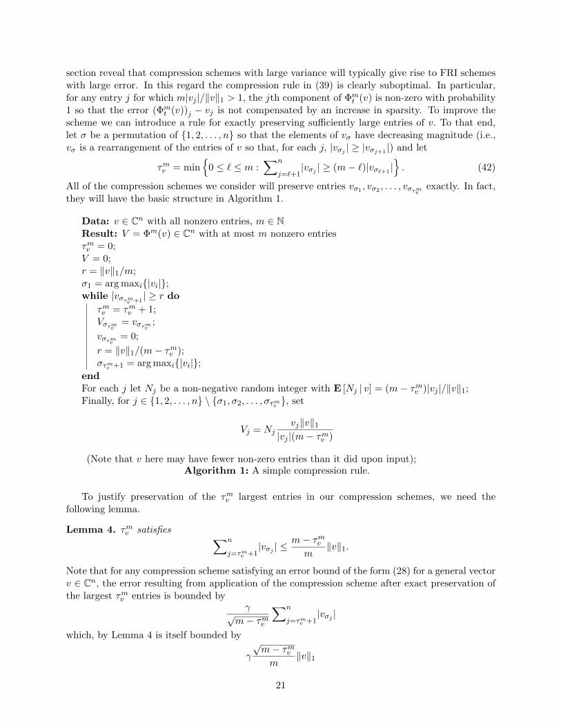
All of the compression schemes we consider will preserve entries vσ1 , vσ2 , . . . , vστmv exactly. In fact,they will have the basic structure in Algorithm 1.

Data: v ∈ Cn with all nonzero entries, m ∈ NResult: V = Φm(v) ∈ Cn with at most m nonzero entriesτmv = 0;V = 0;r = ‖v‖1/m;σ1 = arg maxi{|vi|};while |vστmv +1

| ≥ r do

τmv = τmv + 1;Vστmv = vστmv ;

vστmv = 0;

r = ‖v‖1/(m− τmv );στmv +1 = arg maxi{|vi|};

endFor each j let Nj be a non-negative random integer with E [Nj | v] = (m− τmv )|vj |/‖v‖1;Finally, for j ∈ {1, 2, . . . , n} \ {σ1, σ2, . . . , στmv }, set

Vj = Njvj‖v‖1

|vj |(m− τmv )

(Note that v here may have fewer non-zero entries than it did upon input);Algorithm 1: A simple compression rule.

To justify preservation of the τmv largest entries in our compression schemes, we need thefollowing lemma.

Lemma 4. τmv satisfies ∑n

j=τmv +1|vσj | ≤

m− τmvm

‖v‖1.

Note that for any compression scheme satisfying an error bound of the form (28) for a general vectorv ∈ Cn, the error resulting from application of the compression scheme after exact preservation ofthe largest τmv entries is bounded by

γ√m− τmv

∑n

j=τmv +1|vσj |

which, by Lemma 4 is itself bounded by

γ

√m− τmvm

‖v‖1

21

and is always an improvement over (28).Lemma 5 summarizes the properties of the compression scheme resulting from preserving the

largest τmv entries of an input vector v ∈ Cn exactly and applying (39) with (41) with m replacedby m− τmv to the remaining entries. In particular, Lemma 5 implies that the compression schemesatisfies conditions (28), (29), and (35).

Lemma 5. Let v, w ∈ Cn and assume that v has at most m non-zero entries. For Φmt defined by

Algorithm 1 with (41)

|||Φt(v + w)− v − w||| ≤√

2‖w‖

121 ‖v + w‖

121√

m. (43)

Concerning the size of the resampled vector we have the bound

E[‖Φm

t (v + w)‖21]≤ ‖v + w‖21 + 2

‖v + w‖1‖w‖1m

.

Finally, if τmv+w > 0 then P [Φt(v + w) = 0] = 0. If τmv+w = 0 then

P [Φt(v) = 0] ≤(

min

{‖w‖1‖v + w‖1

,1

e

})m.

In practice this compression scheme would need to be modified to avoid the possibility thatΦmt (v) = 0. As Lemma 5 demonstrates, the probability of this event is extremely small. The issue

can be avoided by simply sampling Φmt (v) until Φm

t (v) 6= 0, i.e., sample Φmt (v) conditioned on the

event {Φmt (v) 6= 0} , and multiplying each entry of the resulting vector by P [Φm

t (v) 6= 0] which canbe computed exactly. A more significant issue is that, while Lemma 5 does guarantee that thecompression scheme just described satisfies (35), the scheme does not guarantee that the numberof non-zero entries in Φm

t (v) does not exceed m as required by Lemma 3 in the last section. Theresults of that section can be modified accordingly or the compression scheme can be modified sothat Φm

t (v) has no more than m non-zero entries (by randomly selecting additional entries to set tozero). Instead of pursuing these modifications here we move on to describe the compression schemeused to generate the results reported in the next section.

Like the compression scheme considered in Lemma 5, the compression scheme used to generatethe results in Section 6 begins with an application of Algorithm 1. To fully specify the scheme weneed to specify the rule used to generate the Nj random variables for j ∈ {σk : k > τmv }. Fork = 1, 2, . . . ,m− τmv , define the random variables

U (k) =1

m− τmv(k − 1 + U) . (44)

where U is a single uniformly chosen random variable on the interval (0,1). We then set

Nσj =∣∣∣{k : U (k)

∑n

j=τmv +1|vσj | ∈ Ij

}∣∣∣ (45)

where we have defined the intervals Iτmv +1 =[0, |vστmv +1

|)

and, for i = τmv + 2, . . . , n,

Ii =[∑i−1

j=τmv +1|vσj |,

∑i

j=τmv +1|vσj |

). (46)

As for the rule in (41), the variables Nj generated according to (45) satisfy

E [Nj | v] =(m− τmv )|vj |∑ni=τmv +1|vσi |

so that the compression mapping Φmt resulting from use of (45) with Algorithm 1 satisfies (30).

From the definition of τmv , we know that for j > τmv , (m − τmv )|vj | ≤∑n

i=τmv +1|vσi | which impliesby (45) that Nj ∈ {0, 1}.

22

Unlike (41), (45) results in Nj that are correlated and satisfy∑n

j=τmv +1Nj = m − τmv exactly(not just in expectation). The corresponding compression scheme exactly preserves the `1-normof v and results in a vector Φm

t (v) with at most m non-zero entries. Note that this compressionscheme, like the one considered in Lemma 5 only requires knowledge of set {σ1, σ2, . . . , στmv } anddoes not require sorting of the entire input vector v. Perhaps the most obvious advantage of thisscheme over the one that generates the Nj according to (41) is that the compression scheme using(45) only requires a single random variate per iteration (compared to up to n for (41)). Dependingon the cost of evaluating M(V m

t ), this advantage could be substantial.Notice that, if we replace the U (k) in (44) by independent random variables uniformly chosen

in (0, 1), then the Nj would be distributed multinomially, which we have already mentioned is apoor choice. Relative to multinomial Nj , the increased correlation between the U (k) defined in (44)results in substantially decreased variance for the Nj but also increased covariance. An unfortunateconsequence of this increased covariance is that the analogue of the error bound (43) from Lemma 5does not hold for Nj generated according to (45). In fact, the rule in (45) is very closely related tothe systematic resampling scheme used frequently in the context of sequential Monte Carlo (see e.g.[15]) which is well known to fail to converge for certain sequences of input vectors.8 Nonetheless,in unreported numerical comparisons we found that the rule (45) resulted in FRI schemes withsignificantly lower error than for (41).

6 Numerical tests

In this section we describe the application of the framework above to particular matrices arisingin (i) the computation of the per-spin partition function of the 2D Ising model, (ii) the spec-tral gap of a diffusion process governing the evolution of a system of up to five, 2-dimensionalparticles (i.e., up to ten spatial dimensions), and (iii) a free energy landscape for that process.The corresponding numerical linear algebra problems are, respectively, (i) computing the domi-nant eigenvalue/eigenvector of matrices up to size 1015 × 1015, (ii) computing the second largesteigenvalue/eigenvector of matrices up to size 1020× 1020, and (iii) solving a linear system involvingexponentiation of matrices up to size 1020×1020. Aside from sparsity, these matrices have no knownreadily exploitable structure for computations.

All but the first test problem involve matrices with entries of any sign. As we learned in Section4, we can often expect much better error scaling with dimension when applying FRI to problemsinvolving matrices with all non-negative entries. The numerical results in this section suggest thatdramatic speedups are possible even for more general matrices.

The reader may wonder why we consider random compressions instead of simple thresholding,i.e., a compression rule in which, if σj is the index of the jth largest (in magnitude) of v, vσj issimply set to zero for all j > m (the resulting vector can be normalized to preserve `1-norm or not).In the rest of this paper we will refer to methods using such a compression rule as truncation-by-size(TbS) schemes. TbS schemes have been considered by many authors (see e.g. [29, 58, 49, 50]) andare a natural approach. Note however that the error (if the compression is not normalized),∣∣∣∑

j>mfσjvσj

∣∣∣ ,for the thresholding compression can be as large as ‖f‖∞‖v‖1 (1−m/n) which only vanishes if m isincreased faster than n. In contrast, the random compressions above can have vanishing error evenwhen n is infinite. This observation is key to understanding the substantial reduction in error wefind for our fast randomized scheme over TbS in numerical results presented in this section. In ourfirst test example the TbS scheme converges to a value far from a high quality estimate of the true

8If applied to the same vector v as m increases, the scheme does converge

23

value (a relative error of 98% compared to 8% for FRI). In the subsequent examples TbS iterationappears to converge (in the iteration index t) to substantially different values for each fixed choiceof m whereas FRI shows much more consistent behavior in m. Moreover, in practice we observe nocost savings per iteration for TbS over FRI.

Finally we comment that, in order for the FRI approach to yield significant performance im-provements, one must use an efficient implementation of matrix by sparse vector multiplication.In the examples below we list the i, j pairs for which the product Kijvj is nonzero, then sort theproducts according to the i-index and finally, add the products with common i. This is a simpleand sub-optimal solution. More details can be found in the example code available in [63].

6.1. A transfer matrix eigenproblem In this example we find the dominant eigenvalue λ∗of the transfer matrix K of the 2-dimensional `-spin Ising model. This eigenvalue is the per-spinpartition function of the infinite spin Ising model, i.e.,

λ∗(T,B) = lim`→∞

(∑σe

1T

∑|(i,j)−(i′,j′)|=1 σijσi′j′+Bσij

)1/`

where σij ∈ {−1, 1} and the sum in the exponent is over pairs of indices on a square 2-dimensional,periodic lattice with ` sites. The outer sum is over all 2` possible values of σ, and for larger `, onecannot possibly compute it directly. The matrix K is 2` × 2`. For example, in the case ` = 3,

K =

a a−1

b b−1

a a−1

b b−1

b b−1

c c−1

b b−1

c c−1

(47)

wherea = e(2−B)/T , b = e−B/T , c = e−(2+B)/T .

We therefore also cannot hope to apply the power method (or its relatives) directly to K when `is large. In our experiments we set T = 2.2, B = 0.01, and ` = 50 so that n = 2` > 1015, Weapply both the FRI and TbS, O(1) schemes to computing λ∗ as well as to computing the sum of allcomponents of the corresponding eigenvector, v∗ (normalized to have sum equal to 1), with indexgreater than or equal to 249, i.e.,

f∗ =∑

j≥n/2(v∗)j .

Knowledge of the partition function λ∗ as a function of temperature T and field strength Ballows one to determine useful quantities such as the average magnetization (sum of spin values)and to diagnose phase transitions [29]. Our choice to estimate λ∗ and f∗ is motivated in part by thefact that these quantities can be approximated accurately by the corresponding values for smallerIsing systems. We will compare our results to those for the 24-spin Ising model which we cansolve by standard power iteration. For an effective specialized method for this problem see [51]. Asimple, educational implementation of Fast Randomized Iteration applied to this problem can befound here [63].

In Figure 1 we report the trajectory averages of the approximations Λmt and Fmt generated bythe FRI scheme (iteration (17) using Algorithm 1) with m = 220, 221, 222, 223, and 224 and 105

total iterations. The best (highest m) approximation of λ∗ is 2.584 and the best approximation off∗ is 0.606. The results for the 24-spin Ising problem are λ∗ ≈ 2.596 and f∗ ≈ 0.658 a differenceof roughly 0.5% and 8% from the respective approximations generated by the FRI method. In

24

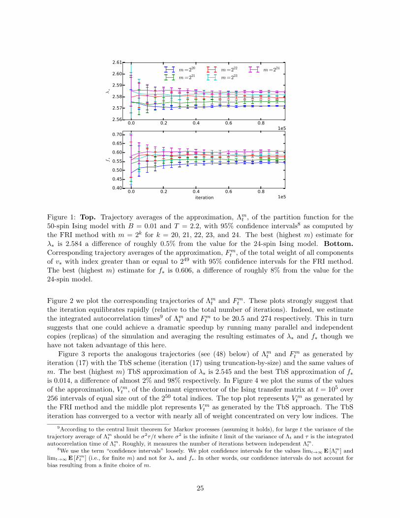
0.0 0.2 0.4 0.6 0.81e5

2.56

2.57

2.58

2.59

2.60

2.61

λ∗

m=220

m=221

m=222

m=223

m=224

0.0 0.2 0.4 0.6 0.8iteration 1e5

0.40

0.45

0.50

0.55

0.60

0.65

0.70

f∗

Figure 1: Top. Trajectory averages of the approximation, Λmt , of the partition function for the50-spin Ising model with B = 0.01 and T = 2.2, with 95% confidence intervals8 as computed bythe FRI method with m = 2k for k = 20, 21, 22, 23, and 24. The best (highest m) estimate forλ∗ is 2.584 a difference of roughly 0.5% from the value for the 24-spin Ising model. Bottom.Corresponding trajectory averages of the approximation, Fmt , of the total weight of all componentsof v∗ with index greater than or equal to 249 with 95% confidence intervals for the FRI method.The best (highest m) estimate for f∗ is 0.606, a difference of roughly 8% from the value for the24-spin model.

Figure 2 we plot the corresponding trajectories of Λmt and Fmt . These plots strongly suggest thatthe iteration equilibrates rapidly (relative to the total number of iterations). Indeed, we estimatethe integrated autocorrelation times9 of Λmt and Fmt to be 20.5 and 274 respectively. This in turnsuggests that one could achieve a dramatic speedup by running many parallel and independentcopies (replicas) of the simulation and averaging the resulting estimates of λ∗ and f∗ though wehave not taken advantage of this here.

Figure 3 reports the analogous trajectories (see (48) below) of Λmt and Fmt as generated byiteration (17) with the TbS scheme (iteration (17) using truncation-by-size) and the same values ofm. The best (highest m) TbS approximation of λ∗ is 2.545 and the best TbS approximation of f∗is 0.014, a difference of almost 2% and 98% respectively. In Figure 4 we plot the sums of the valuesof the approximation, V m

t , of the dominant eigenvector of the Ising transfer matrix at t = 105 over256 intervals of equal size out of the 250 total indices. The top plot represents V m

t as generated bythe FRI method and the middle plot represents V m

t as generated by the TbS approach. The TbSiteration has converged to a vector with nearly all of weight concentrated on very low indices. The

9According to the central limit theorem for Markov processes (assuming it holds), for large t the variance of thetrajectory average of Λmt should be σ2τ/t where σ2 is the infinite t limit of the variance of Λt and τ is the integratedautocorrelation time of Λmt . Roughly, it measures the number of iterations between independent Λmt .

8We use the term “confidence intervals” loosely. We plot confidence intervals for the values limt→∞E [Λmt ] andlimt→∞E [Fmt ] (i.e., for finite m) and not for λ∗ and f∗. In other words, our confidence intervals do not account forbias resulting from a finite choice of m.

25

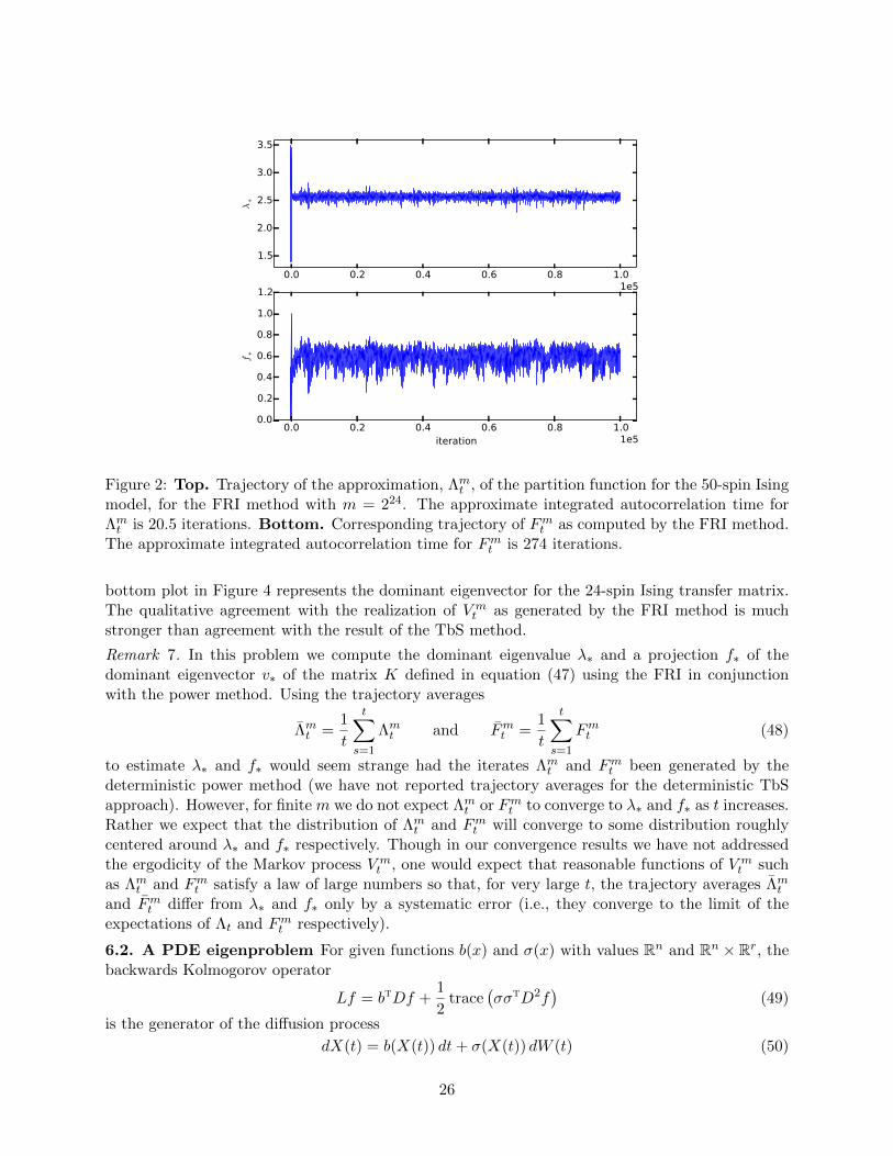
0.0 0.2 0.4 0.6 0.8 1.01e5

1.5

2.0

2.5

3.0

3.5

λ∗

0.0 0.2 0.4 0.6 0.8 1.0iteration 1e5

0.0

0.2

0.4

0.6

0.8

1.0

1.2

f∗

Figure 2: Top. Trajectory of the approximation, Λmt , of the partition function for the 50-spin Isingmodel, for the FRI method with m = 224. The approximate integrated autocorrelation time forΛmt is 20.5 iterations. Bottom. Corresponding trajectory of Fmt as computed by the FRI method.The approximate integrated autocorrelation time for Fmt is 274 iterations.

bottom plot in Figure 4 represents the dominant eigenvector for the 24-spin Ising transfer matrix.The qualitative agreement with the realization of V m

t as generated by the FRI method is muchstronger than agreement with the result of the TbS method.

Remark 7. In this problem we compute the dominant eigenvalue λ∗ and a projection f∗ of thedominant eigenvector v∗ of the matrix K defined in equation (47) using the FRI in conjunctionwith the power method. Using the trajectory averages

Λmt =1

t

t∑s=1

Λmt and Fmt =1

t

t∑s=1

Fmt (48)

to estimate λ∗ and f∗ would seem strange had the iterates Λmt and Fmt been generated by thedeterministic power method (we have not reported trajectory averages for the deterministic TbSapproach). However, for finite m we do not expect Λmt or Fmt to converge to λ∗ and f∗ as t increases.Rather we expect that the distribution of Λmt and Fmt will converge to some distribution roughlycentered around λ∗ and f∗ respectively. Though in our convergence results we have not addressedthe ergodicity of the Markov process V m

t , one would expect that reasonable functions of V mt such

as Λmt and Fmt satisfy a law of large numbers so that, for very large t, the trajectory averages Λmtand Fmt differ from λ∗ and f∗ only by a systematic error (i.e., they converge to the limit of theexpectations of Λt and Fmt respectively).

6.2. A PDE eigenproblem For given functions b(x) and σ(x) with values Rn and Rn × Rr, thebackwards Kolmogorov operator

Lf = btDf +1

2trace

(σσtD2f

)(49)

is the generator of the diffusion process

dX(t) = b(X(t)) dt+ σ(X(t)) dW (t) (50)

26

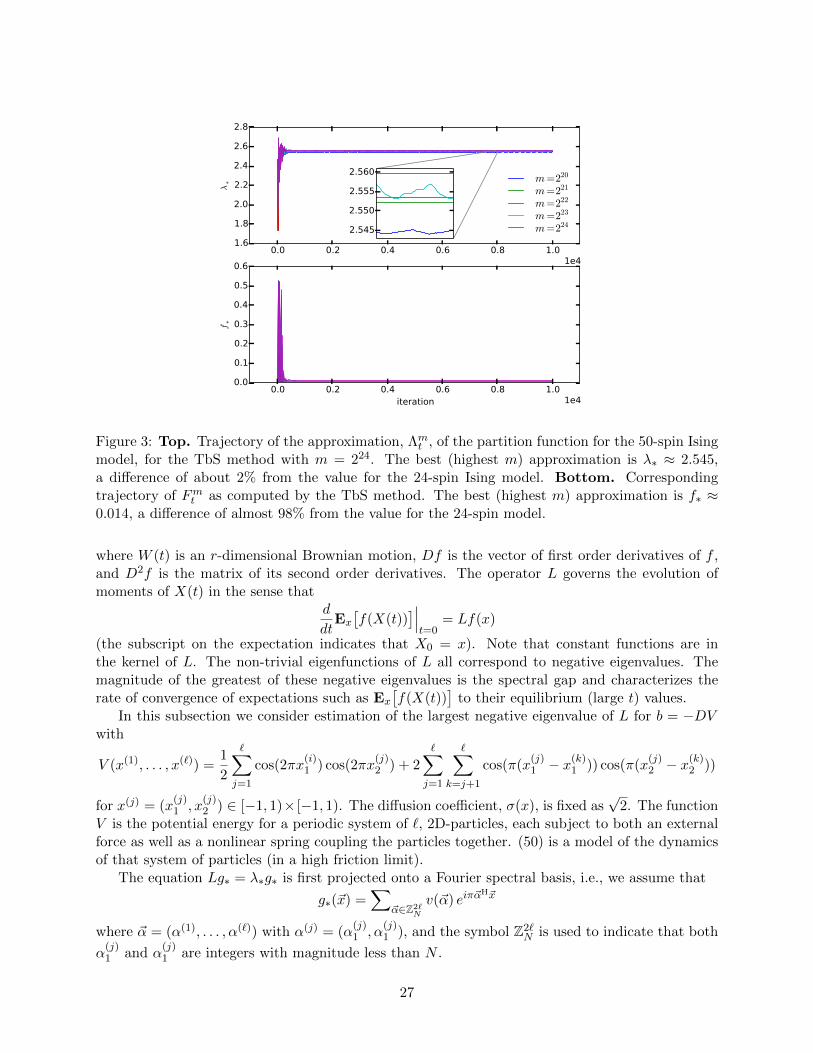
0.0 0.2 0.4 0.6 0.8 1.01e4

1.6

1.8

2.0

2.2

2.4

2.6

2.8

λ∗ m=220

m=221

m=222

m=223

m=2242.545

2.550

2.555

2.560

0.0 0.2 0.4 0.6 0.8 1.0iteration 1e4

0.0

0.1

0.2

0.3

0.4

0.5

0.6

f∗

Figure 3: Top. Trajectory of the approximation, Λmt , of the partition function for the 50-spin Isingmodel, for the TbS method with m = 224. The best (highest m) approximation is λ∗ ≈ 2.545,a difference of about 2% from the value for the 24-spin Ising model. Bottom. Correspondingtrajectory of Fmt as computed by the TbS method. The best (highest m) approximation is f∗ ≈0.014, a difference of almost 98% from the value for the 24-spin model.

where W (t) is an r-dimensional Brownian motion, Df is the vector of first order derivatives of f ,and D2f is the matrix of its second order derivatives. The operator L governs the evolution ofmoments of X(t) in the sense that

d

dtEx[f(X(t))

]∣∣∣t=0

= Lf(x)

(the subscript on the expectation indicates that X0 = x). Note that constant functions are inthe kernel of L. The non-trivial eigenfunctions of L all correspond to negative eigenvalues. Themagnitude of the greatest of these negative eigenvalues is the spectral gap and characterizes therate of convergence of expectations such as Ex

[f(X(t))

]to their equilibrium (large t) values.

In this subsection we consider estimation of the largest negative eigenvalue of L for b = −DVwith

V (x(1), . . . , x(`)) =1

2

∑j=1

cos(2πx(i)1 ) cos(2πx

(j)2 ) + 2

∑j=1

∑k=j+1

cos(π(x(j)1 − x

(k)1 )) cos(π(x

(j)2 − x

(k)2 ))

for x(j) = (x(j)1 , x

(j)2 ) ∈ [−1, 1)× [−1, 1). The diffusion coefficient, σ(x), is fixed as

√2. The function

V is the potential energy for a periodic system of `, 2D-particles, each subject to both an externalforce as well as a nonlinear spring coupling the particles together. (50) is a model of the dynamicsof that system of particles (in a high friction limit).

The equation Lg∗ = λ∗g∗ is first projected onto a Fourier spectral basis, i.e., we assume that

g∗(~x) =∑

~α∈Z2`N

v(~α) eiπ~αH~x

where ~α = (α(1), . . . , α(`)) with α(j) = (α(j)1 , α

(j)1 ), and the symbol Z2`

N is used to indicate that both

α(j)1 and α

(j)1 are integers with magnitude less than N .

27

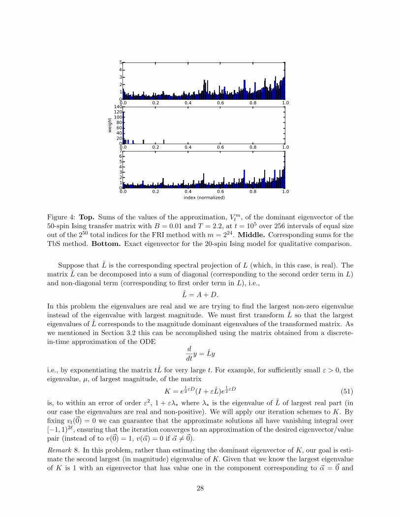
0.0 0.2 0.4 0.6 0.8 1.00

1

2

3

4

5

0.0 0.2 0.4 0.6 0.8 1.00

20406080

100120140

weig

ht

0.0 0.2 0.4 0.6 0.8 1.0index (normalized)

01234567

Figure 4: Top. Sums of the values of the approximation, V mt , of the dominant eigenvector of the

50-spin Ising transfer matrix with B = 0.01 and T = 2.2, at t = 105 over 256 intervals of equal sizeout of the 250 total indices for the FRI method with m = 224. Middle. Corresponding sums for theTbS method. Bottom. Exact eigenvector for the 20-spin Ising model for qualitative comparison.

Suppose that L is the corresponding spectral projection of L (which, in this case, is real). Thematrix L can be decomposed into a sum of diagonal (corresponding to the second order term in L)and non-diagonal term (corresponding to first order term in L), i.e.,

L = A+D.

In this problem the eigenvalues are real and we are trying to find the largest non-zero eigenvalueinstead of the eigenvalue with largest magnitude. We must first transform L so that the largesteigenvalues of L corresponds to the magnitude dominant eigenvalues of the transformed matrix. Aswe mentioned in Section 3.2 this can be accomplished using the matrix obtained from a discrete-in-time approximation of the ODE

d

dty = Ly

i.e., by exponentiating the matrix tL for very large t. For example, for sufficiently small ε > 0, theeigenvalue, µ, of largest magnitude, of the matrix

K = e12εD(I + εL)e

12εD (51)

is, to within an error of order ε2, 1 + ελ∗ where λ∗ is the eigenvalue of L of largest real part (inour case the eigenvalues are real and non-positive). We will apply our iteration schemes to K. Byfixing vt(~0) = 0 we can guarantee that the approximate solutions all have vanishing integral over[−1, 1)2`, ensuring that the iteration converges to an approximation of the desired eigenvector/valuepair (instead of to v(~0) = 1, v(~α) = 0 if ~α 6= ~0).

Remark 8. In this problem, rather than estimating the dominant eigenvector of K, our goal is esti-mate the second largest (in magnitude) eigenvalue of K. Given that we know the largest eigenvalueof K is 1 with an eigenvector that has value one in the component corresponding to ~α = ~0 and

28

zeros in all other components, we can therefore exactly orthogonalize the iterates V mt with respect

to the dominant eigenvalue at each iteration (by fixing V mt (~0) = 0). We may view this as using

FRI in conjunction with a simple case of orthogonal iteration.

We compare the FRI and TbS approaches with N = 51 for the four- and five-particle systems(` = 4, 5). The corresponding total count of real numbers needed to represent the solution in thefive-particle case is 10110 ≈ 1020 so only the O(1) scheme is reasonable. For h we choose a valueof 10−3. Our potential V is chosen so that the resulting matrix L (and therefore also K) is sparseand its entries are computed by hand. For a more complicated V , the entries of L might have tobe computed numerically on-the-fly or might not be computable at all. Our ability to efficientlycompute the entries of L will be strongly effected by the choice of basis. For example, if we use afinite difference approximation of L then the entries of L can be computed easily. On the other hand,if the solution is reasonably smooth, the finite difference approximation will converge much moreslowly than an approximation (like the spectral approximation) that more directly incorporatesproperties of the solution (regularity in this case).

Figure 5 plots the trajectory averages over 105 iterations for Λmt in the ` = 4 case generatedby the FRI method (iteration (17) using Algorithm 1) along with corresponding trajectories of Λmtas generated by the TbS approach (iteration (17) using truncation-by-size). We present resultsfor both methods with m = 1, 2, 3, and 4 × 104. Observe that the results from the FRI methodappear to have converged on one another while the results generated by the TbS approach show nosigns of convergence. The best (highest m) estimate of the eigenvalue generated by FRI is −2.31and the best estimate generated by TbS is −2.49. Figure 6 plots the trajectory of Λmt in the fiveparticle (` = 5) case as generated by the FRI method with m = 106 along with its trajectoryaverage (neglecting the first 500 iterations) of about −1.3. Note that Λmt appears to reach itsstatistical equilibrium rapidly relative to the 2×103 total iterations. Again, the rapid equilibrationsuggests that statistical error could be removed by averaging over many shorter trajectories evolvedin parallel.

6.3. A PDE steady state problem The adjoint L∗ of the operator defined in (49) with respectto the standard inner product is called the Fokker–Planck operator. The operator determines theevolution of the density of the process X(t) defined in (50) in the sense that if µ is that densitythen

∂tµ = L∗µ.

An element in the kernel of L∗ (a steady state solution of the Fokker–Planck equation) is a densityleft invariant by X(t).

For the choice of b and σ given in the previous subsection, the steady state solutions are easilyseen to be constant multiples of the function

µ∗(~x) =e−V (~x)∫e−V (~x)

.

In most applications, the goal is to compute averages of observables with respect to µ∗. Forexample, one might hope to find (up to an additive constant) the effective potential (or free-energy)experienced by particle 1,

F1(x(1)) = − log

∫µ∗(~x) dx(2) · · · dx(`).

For that purpose, explicit knowledge of µ∗ is of little value since one cannot hope to computeintegrals with respect to a function of so many variables (up to 1018 in our tests). One insteadhopes to find a more digestible expression for µ∗. Notice that if a Fourier expansion

µ∗(~x) =∑

~α∈Z2`N

v(~j) eiπ~αH~x

29

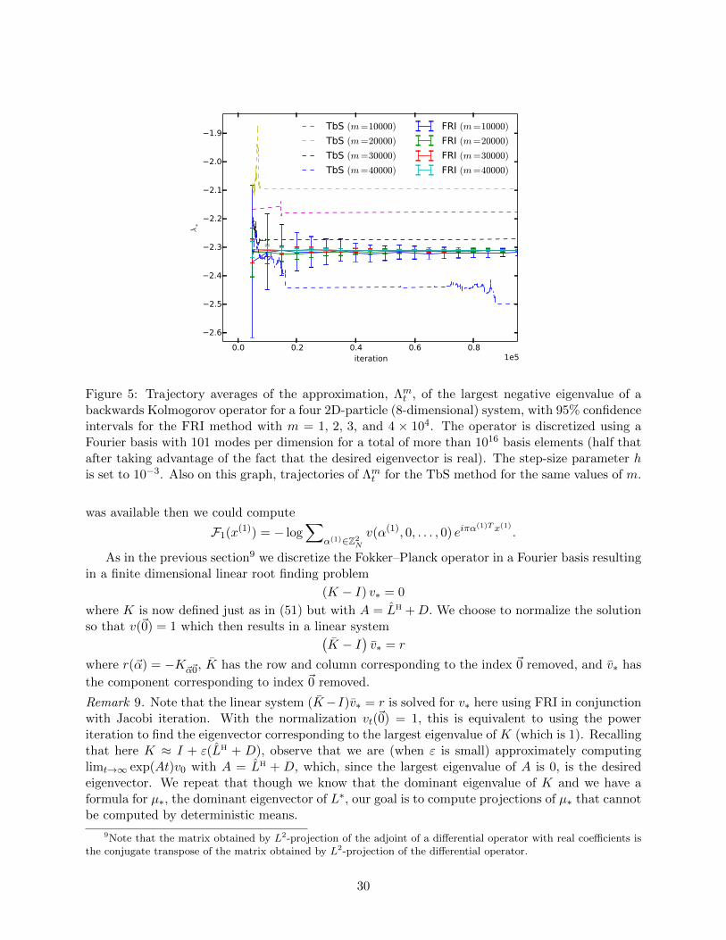
0.0 0.2 0.4 0.6 0.8iteration 1e5

2.6

2.5

2.4

2.3

2.2

2.1

2.0

1.9

λ∗

TbS (m=10000)

TbS (m=20000)

TbS (m=30000)

TbS (m=40000)

FRI (m=10000)

FRI (m=20000)

FRI (m=30000)

FRI (m=40000)

Figure 5: Trajectory averages of the approximation, Λmt , of the largest negative eigenvalue of abackwards Kolmogorov operator for a four 2D-particle (8-dimensional) system, with 95% confidenceintervals for the FRI method with m = 1, 2, 3, and 4 × 104. The operator is discretized using aFourier basis with 101 modes per dimension for a total of more than 1016 basis elements (half thatafter taking advantage of the fact that the desired eigenvector is real). The step-size parameter his set to 10−3. Also on this graph, trajectories of Λmt for the TbS method for the same values of m.

was available then we could compute

F1(x(1)) = − log∑

α(1)∈Z2N

v(α(1), 0, . . . , 0) eiπα(1)T x(1) .

As in the previous section9 we discretize the Fokker–Planck operator in a Fourier basis resultingin a finite dimensional linear root finding problem

(K − I) v∗ = 0

where K is now defined just as in (51) but with A = LH +D. We choose to normalize the solutionso that v(~0) = 1 which then results in a linear system(

K − I)v∗ = r

where r(~α) = −K~α~0, K has the row and column corresponding to the index ~0 removed, and v∗ has

the component corresponding to index ~0 removed.

Remark 9. Note that the linear system (K−I)v∗ = r is solved for v∗ here using FRI in conjunctionwith Jacobi iteration. With the normalization vt(~0) = 1, this is equivalent to using the poweriteration to find the eigenvector corresponding to the largest eigenvalue of K (which is 1). Recallingthat here K ≈ I + ε(LH + D), observe that we are (when ε is small) approximately computinglimt→∞ exp(At)v0 with A = LH + D, which, since the largest eigenvalue of A is 0, is the desiredeigenvector. We repeat that though we know that the dominant eigenvalue of K and we have aformula for µ∗, the dominant eigenvector of L∗, our goal is to compute projections of µ∗ that cannotbe computed by deterministic means.

9Note that the matrix obtained by L2-projection of the adjoint of a differential operator with real coefficients isthe conjugate transpose of the matrix obtained by L2-projection of the differential operator.

30

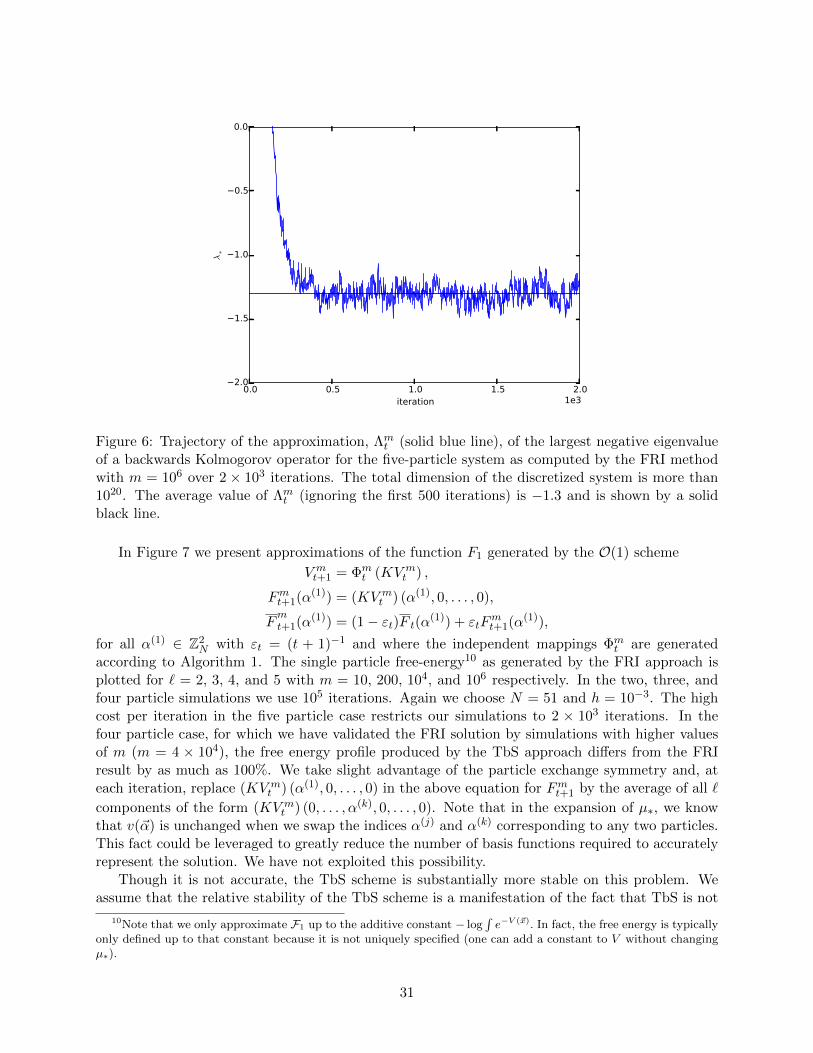
0.0 0.5 1.0 1.5 2.0iteration 1e3

2.0

1.5

1.0

0.5

0.0

λ∗

Figure 6: Trajectory of the approximation, Λmt (solid blue line), of the largest negative eigenvalueof a backwards Kolmogorov operator for the five-particle system as computed by the FRI methodwith m = 106 over 2 × 103 iterations. The total dimension of the discretized system is more than1020. The average value of Λmt (ignoring the first 500 iterations) is −1.3 and is shown by a solidblack line.

In Figure 7 we present approximations of the function F1 generated by the O(1) scheme

V mt+1 = Φm

t (KV mt ) ,

Fmt+1(α(1)) = (KV mt ) (α(1), 0, . . . , 0),

Fmt+1(α(1)) = (1− εt)F t(α(1)) + εtF

mt+1(α(1)),

for all α(1) ∈ Z2N with εt = (t + 1)−1 and where the independent mappings Φm

t are generatedaccording to Algorithm 1. The single particle free-energy10 as generated by the FRI approach isplotted for ` = 2, 3, 4, and 5 with m = 10, 200, 104, and 106 respectively. In the two, three, andfour particle simulations we use 105 iterations. Again we choose N = 51 and h = 10−3. The highcost per iteration in the five particle case restricts our simulations to 2 × 103 iterations. In thefour particle case, for which we have validated the FRI solution by simulations with higher valuesof m (m = 4 × 104), the free energy profile produced by the TbS approach differs from the FRIresult by as much as 100%. We take slight advantage of the particle exchange symmetry and, ateach iteration, replace (KV m

t ) (α(1), 0, . . . , 0) in the above equation for Fmt+1 by the average of all `

components of the form (KV mt ) (0, . . . , α(k), 0, . . . , 0). Note that in the expansion of µ∗, we know

that v(~α) is unchanged when we swap the indices α(j) and α(k) corresponding to any two particles.This fact could be leveraged to greatly reduce the number of basis functions required to accuratelyrepresent the solution. We have not exploited this possibility.

Though it is not accurate, the TbS scheme is substantially more stable on this problem. Weassume that the relative stability of the TbS scheme is a manifestation of the fact that TbS is not

10Note that we only approximate F1 up to the additive constant − log∫e−V (~x). In fact, the free energy is typically

only defined up to that constant because it is not uniquely specified (one can add a constant to V without changingµ∗).

31

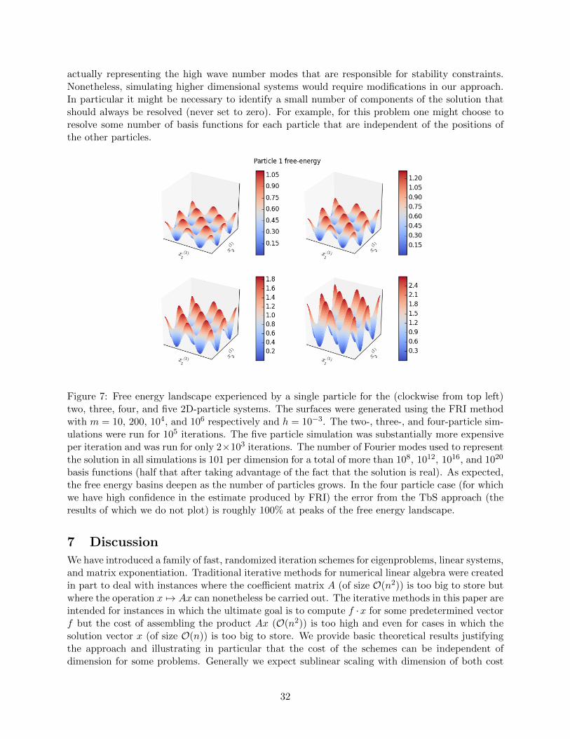
actually representing the high wave number modes that are responsible for stability constraints.Nonetheless, simulating higher dimensional systems would require modifications in our approach.In particular it might be necessary to identify a small number of components of the solution thatshould always be resolved (never set to zero). For example, for this problem one might choose toresolve some number of basis functions for each particle that are independent of the positions ofthe other particles.

Figure 7: Free energy landscape experienced by a single particle for the (clockwise from top left)two, three, four, and five 2D-particle systems. The surfaces were generated using the FRI methodwith m = 10, 200, 104, and 106 respectively and h = 10−3. The two-, three-, and four-particle sim-ulations were run for 105 iterations. The five particle simulation was substantially more expensiveper iteration and was run for only 2×103 iterations. The number of Fourier modes used to representthe solution in all simulations is 101 per dimension for a total of more than 108, 1012, 1016, and 1020

basis functions (half that after taking advantage of the fact that the solution is real). As expected,the free energy basins deepen as the number of particles grows. In the four particle case (for whichwe have high confidence in the estimate produced by FRI) the error from the TbS approach (theresults of which we do not plot) is roughly 100% at peaks of the free energy landscape.

7 Discussion

We have introduced a family of fast, randomized iteration schemes for eigenproblems, linear systems,and matrix exponentiation. Traditional iterative methods for numerical linear algebra were createdin part to deal with instances where the coefficient matrix A (of size O(n2)) is too big to store butwhere the operation x 7→ Ax can nonetheless be carried out. The iterative methods in this paper areintended for instances in which the ultimate goal is to compute f ·x for some predetermined vectorf but the cost of assembling the product Ax (O(n2)) is too high and even for cases in which thesolution vector x (of size O(n)) is too big to store. We provide basic theoretical results justifyingthe approach and illustrating in particular that the cost of the schemes can be independent ofdimension for some problems. Generally we expect sublinear scaling with dimension of both cost

32

and storage requirements as observed in our numerical experiments. The identification of generalconditions guaranteeing sublinear scaling for FRI schemes is not addressed in this article but seemsa very interesting direction for future research.

A completely deterministic approach to iterative problems related to the methods proposed inthis article is the simple thresholding by size (TbS) in which, at each iteration, the smallest entriesin the approximation are set to zero. An adaptive version of the TbS approach has recently beenadvocated for a wide range of applications (see [58, 49, 50]). Like TbS our randomized schemes alsorely on the enforcement of sparsity and also tend to set small entries in the approximate solutionto zero. While the TbS approach can be effective on some problems with sparse solutions, theirerror in general will be strongly dependent on system size and we find that it performs very poorlyon our test problems relative to FRI.

The core concept behind the FRI schemes introduced in this article is the notion that, byrandomly setting entries in vectors to zero, while maintaining a statistical consistency property,we can dramatically reduce the cost and storage of standard iterative schemes. One can viewour FRI schemes as an attempt to blur the line separating Markov chain Monte Carlo (MCMC),which is effective in extremely high dimensional settings but is limited to a relatively narrow classof problems and often does not allow the user to take full advantage of known properties of thesolution (e.g. smoothness or symmetry properties as in [7]), and traditional deterministic schemes,which are effective on a very general set of relatively low dimensional problems. As for MCMCapproaches, if one settles for computing low dimensional projections of the full solution then notevery element of the state space need be visited and effective FRI schemes with per iteration costand storage requirements independent of system size can be derived (as for MCMC the validity ofthis statement depends on the particular sequence of problems considered). Also as for MCMCwe expect that, when deterministic alternatives are available, they will outperform our randomizedschemes. For matrices of the size considered in all of our numerical tests, deterministic alternativesare not available.

Experience with diffusion Monte Carlo in the context of quantum Monte Carlo simulationssuggests that our randomized schemes will be most useful if applied after considerable effort hasbeen expended on finding changes of variables that either make the desired solution as sparse aspossible (reducing both bias and variance) or reduce bias by some other means. In many cases thiswill mean applying our randomized schemes only after one has obtained an estimate of the solutionby some deterministic method applied to a reduced dimensional version of the target problem.

Acknowledgments

JQW would like to thank Eric Cances, Tony Lelievre, and Matthias Rousset, for their hospitalityand helpful discussions during a visit to ENPC that coincided with the early stages of this work.Both authors would like to thank Mihai Anitescu, Alexandre Chorin, Petros Drineas, Risi Kondor,Jianfeng Lu, Omiros Papaspiliopoulos, Panos Stinis, and the anonymous referees, who all madecomments that strongly affected this article’s structure and content. LHL’s work is generouslysupported by DARPA D15AP00109, AFOSR FA9550-13-1-0133, NSF IIS-1546413, DMS-1209136,and DMS-1057064. JQW’s effort was supported by the Advance Scientific Computing Researchprogram within the DOE Office of Science through award de-sc0014205 as well as through a contractfrom Argonne, a U.S. Department of Energy Office of Science laboratory.

References

[1] V.N. Alexandrov and S. Lakka. Comparison of three monte carlo methods for matrix inversion.In Luc Bouge, Pierre Fraigniaud, Anne Mignotte, and Yves Robert, editors, Euro-Par’96

33

Parallel Processing, volume 1124 of Lecture Notes in Computer Science, pages 72–80. SpringerBerlin Heidelberg, 1996.

[2] J. Anderson. A random-walk simulation of the Schrodinger equation: H+3 . J. Chem. Phys.,

63(4):1499–1503, 1975.

[3] Roi Baer, Daniel Neuhauser, and Eran Rabani. Self-averaging stochastic kohn-sham density-functional theory. Phys. Rev. Lett., 111:106402, Sep 2013.

[4] George H. Booth and Ali Alavi. Approaching chemical accuracy using full configuration in-teraction quantum monte carlo: a study of ionization potentials. J. Chem. Phys., 132:174104,2010.

[5] George H. Booth, D. Cleland, Alex J. W. Thom, and Ali Alavi. Breaking the carbon dimer:the challenges of multiple bond dissociation with full configuration interaction quantum MonteCarlo methods. J. Chem. Phys., 135:084104, 2011.

[6] George H. Booth, Andreas Gruneis, Georg Kresse, and Ali Alavi. Towards an exact descriptionof electronic wavefunctions in real solids. Nature, 493(7432):365–370, 01 2013.

[7] George H. Booth, Alex J. W. Thom, and Ali Alavi. Fermion monte carlo without fixed nodes:A game of life, death, and annihilation in slater determinant space. The Journal of ChemicalPhysics, 131(5), 2009.

[8] Leon Bottou. Stochastic learning. In Olivier Bousquet and Ulrike von Luxburg, editors,Advanced Lectures on Machine Learning, Lecture Notes in Artificial Intelligence, LNAI 3176,pages 146–168. Springer Verlag, Berlin, 2004.

[9] N. Bou-Rabee and E. Vanden-Eijnden. Continuous-time random walks for the numericalsolution of stochastic differential equations. arXiv:1502.05034 [math.PR], 2015.

[10] D. Ceperley and B. Alder. Ground state of electron gas by a stochastic method. Phys. Rev.Lett., 45(7):566–569, 1980.

[11] Alexandre Chorin. Random choice solution of hyperbolic systems. Journal of ComputationalPhysics, 22:517–536, 1976.

[12] D. Cleland, George H. Booth, and Ali Alavi. Survival of the fittest: accelerating convergencein full configuration-interaction quantum Monte Carlo. J. Chem. Phys., 132:041103, 2010.

[13] D. Cleland, George H. Booth, and Ali Alavi. A study of electron affinities using the initiatorapproach to full configuration interaction quantum Monte Carlo. J. Chem. Phys., 134:024112,2011.

[14] E. Coakley, V. Rokhlin, and M. Tygert. A fast randomized algorithm for orthogonal projection.SIAM Journal on Scientific Computing, 33(2):849–868, 2011.

[15] N. de Freitas, A. Doucet, and N. Gordon (Eds). Sequential Monte Carlo Methods in Practice.Springer, 2005.

[16] Pierre Del Moral. Feynman-Kac formulae. Probability and its Applications (New York).Springer-Verlag, New York, 2004. Genealogical and interacting particle systems with applica-tions.

34

[17] James W. Demmel. Applied Numerical Linear Algebra. Society for Industrial and AppliedMathematics, 1997.

[18] I.T. Dimov, T.T. Dimov, and T.V. Gurov. A new iterative monte carlo approach for inversematrix problem. Journal of Computational and Applied Mathematics, 92(1):15 – 35, 1998.

[19] I.T. Dimov, A.N. Karaivanova, and P.I. Yordanova. Monte carlo algorithms for calculatingeigenvalues. In Harald Niederreiter, Peter Hellekalek, Gerhard Larcher, and Peter Zinterhof,editors, Monte Carlo and Quasi-Monte Carlo Methods 1996, volume 127 of Lecture Notes inStatistics, pages 205–220. Springer New York, 1998.

[20] P. Drineas, R. Kannan, and M. Mahoney. Fast Monte Carlo algorithms for matrices I: Ap-proximating matrix multiplication. SIAM Journal on Computing, 36(1):132–157, 2006.

[21] P. Drineas, R. Kannan, and M. Mahoney. Fast Monte Carlo algorithms for matrices II: Com-puting a low-rank approximation to a matrix. SIAM Journal on Computing, 36(1):158–183,2006.

[22] P. Drineas, R. Kannan, and M. Mahoney. Fast Monte Carlo algorithms for matrices III:Computing a compressed approximate matrix decomposition. SIAM Journal on Computing,36(1):184–206, 2006.

[23] Weinan E, Bjorn Engquist, Xiantao Li, Weiqing Ren, and Eric Vanden-Eijnden. The heterog-nous multiscale methods: A review. Communications in Computational Physics, 2(3):367–450,06 2007.

[24] Sylvester Eriksson-Bique, Mary Solbrig, Michael Stefanelli, Sarah Warkentin, Ralph Abbey,and Ilse C. F. Ipsen. Importance sampling for a Monte Carlo matrix multiplication algorithm,with application to information retrieval. SIAM J. Sci. Comput., 33(4):1689–1706, July 2011.

[25] G. E. Forsythe and R. A. Leibler. Matrix inverstion by a Monte Carlo method. MathematicalTables and Aids to Computation, 4(127-129), 1950.

[26] W. Foulkes, L. Mitas, R. Needs, and G. Rajagopal. Quantum Monte Carlo simulations ofsolids. Rev. Mod. Phys., 73(1):33–79, 2001.

[27] S. Friedland and L.-H. Lim. Nuclear norm of higher-order tensors. Math. Comp., 2016. toappear.

[28] Alan Frieze, Ravi Kannan, and Santosh Vempala. Fast monte-carlo algorithms for findinglow-rank approximations. J. ACM, 51(6):1025–1041, November 2004.

[29] Norman H. Fuchs. Approximate solutions for large transfer matrix problems. Journal ofComputational Physics, 83(1):201 – 211, 1989.

[30] J. Goodman and N. Madras. Random-walk interpretations of classical iteration methods.Linear Algebra Appl., 216:61–79, 1995.

[31] N. Gordon, D. Salmond, and A. Smith. Novel approach to nonlinear non-Gaussian Bayesianstate estimation. IEE Proceedings F, 51:107 – 113, 1993.

[32] R. Grimm and R. Storer. Monte-Carlo solution of Schrodinger’s equation. J. Comp. Phys.,7(1):134–156, 1971.

35

[33] Martin Hairer and Jonathan Weare. Improved diffusion Monte Carlo. Commun. Pure Appl.Math., 67:1995—2021, 2014.

[34] John H. Halton. Sequential Monte Carlo. In Proceedings of the Cambridge PhilosophicalSociety, volume 58, pages 57–78, 1962.

[35] John H. Halton. A retrospective and prospective survey of the monte carlo method. SIAMReview, 12(1):1–63, 1970.

[36] John H. Halton. Sequential monte carlo techniques for the solution of linear systems. Journalof Scientific Computing, 9(2):213–257, 1994.

[37] J. M. Hammersley. Monte carlo methods for solving multivariable problems. Annals of theNew York Academy of Sciences, 86(3):844–874, 1960.

[38] J. M. Hammersley and D. C. Handscomb. Monte Carlo Methods. Methuen and Co., Londonand John Wiley and Sons, New York, 1964.

[39] J.M. Hammersley and K.W. Morton. Poor man’s Monte Carlo. J. R. Stat. Soc. B, 16(1):23–38,1954.

[40] M. Kalos. Monte Carlo calculations of the ground state of three- and four-body nuclei. Phys.Rev., 128(4):1791–1795, 1962.

[41] G. Kitagawa. Monte Carlo filter and smoother for non-Gaussian nonlinear state space models.Journal of Computational and Graphical Statistics, 5:1–25, 1996.

[42] J. Kolorenc and L. Mitas. Applications of quantum Monte Carlo methods in condensed sys-tems. Rep. Prog. Phys., 74:1–28, 2011.

[43] H. Kushner and G. Yin. Stochastic Approximation and Recursive Algorithms and Applications,volume 35 of Stochastic Modelling and Applied Probability. Springer, 2nd edition, 2003.

[44] Edo Liberty, Franco Woolfe, Per-Gunnar Martinsson, Vladimir Rokhlin, and Mark Tygert.Randomized algorithms for the low-rank approximation of matrices. Proceedings of the Na-tional Academy of Sciences, 104(51):20167–20172, 2007.

[45] P. Lopez Rıos, A. Ma, N. D. Drummond, M. D. Towler, and R. J. Needs. Inhomogeneousbackflow transformations in quantum monte carlo calculations. Phys. Rev. E, 74:066701, Dec2006.

[46] Per-Gunnar Martinsson, Vladimir Rokhlin, and Mark Tygert. A randomized algorithm forthe decomposition of matrices. Applied and Computational Harmonic Analysis, 30(1):47 – 68,2011.

[47] Eric Moulines and Francis R. Bach. Non-asymptotic analysis of stochastic approximationalgorithms for machine learning. In J. Shawe-Taylor, R.S. Zemel, P.L. Bartlett, F. Pereira,and K.Q. Weinberger, editors, Advances in Neural Information Processing Systems 24, pages451–459. Curran Associates, Inc., 2011.

[48] M. P. Nightingale and H. W. J. Blote. Gap of the linear spin-1 heisenberg antiferromagnet: Amonte carlo calculation. Phys. Rev. B, 33:659–661, Jan 1986.

36

[49] Vidvuds Ozolins, Rongjie Lai, Russel Caflisch, and Stanley Osher. Compressed modes forvariational problems in mathematics and physics. Proceedings of the National Academy ofSciences, 110(46):18368–18373, 2013.

[50] Vidvuds Ozolins, Rongjie Lai, Russel Caflisch, and Stanley Osher. Compressed plane wavesyield a compactly supported multiresolution basis for the laplace operator. Proceedings of theNational Academy of Sciences, 111(5):1691–1696, 2014.

[51] B. Parlett and Wee-Liang Heng. The method of minimal representations in 2D Ising modelcalculations. Journal of Computational Physics, 114:257–264, 1994.

[52] G.A. Pavliotis and A.M. Stuart. Multiscale Methods: Averaging and Homogenization, vol-ume 53 of Texts in Applied Mathematics. Springer, 2008.

[53] Herbert Robbins and Sutton Monro. A stochastic approximation method. The Annals ofMathematical Statistics, 22(3):400–407, 1951.

[54] Vladimir Rokhlin, Arthur Szlam, and Mark Tygert. A randomized algorithm for principalcomponent analysis. SIAM J. Matrix Anal. Appl., 31(3):1100–1124, August 2009.

[55] Vladimir Rokhlin and Mark Tygert. A fast randomized algorithm for overdetermined linearleast-squares regression. Proceedings of the National Academy of Sciences, 105(36):13212–13217, 2008.

[56] M.N. Rosenbluth and A.W. Rosenbluth. Monte Carlo calculation of the average extension ofmolecular chains. J. Chem. Phys., 23(2):356–359, 1955.

[57] Mathias Rousset. On the control of an interacting particle approximation of schrodinger groundstates. SIAM J. Math. Anal, 38(3):824–844, 2006.

[58] Hayden Schaeffer, Russel Caflisch, Cory D. Hauck, and Stanley Osher. Sparse dynamics forpartial differential equations. Proceedings of the National Academy of Sciences, 110(17):6634–6639, 2013.

[59] J.J. Sheperd, George H. Booth, A. Gruneis, and Ali Alavi. Full configuration interactionperspective on the homogeneous electron gas. Phys. Rev. B, 85, 2012.

[60] G. W. Stewart. Matrix Algorithms II: Eigensystems. SIAM, 2001.

[61] Thomas Strohmer and Roman Vershynin. A randomized kaczmarz algorithm with exponentialconvergence. Journal of Fourier Analysis and Applications, 15(2):262–278, 2008.

[62] W. R. Wasow. A note on the inversion of matrices by random walk. Mathematical Tables andAids to Computation, 6(78-81), 1952.

[63] Jonathan Weare. A simple example in C++ of FRI applied to computing the dominanteigenvalue of a matrix. http://dx.doi.org/10.5281/zenodo.31208, 2015.

[64] Franco Woolfe, Edo Liberty, Vladimir Rokhlin, and Mark Tygert. A fast randomized algorithmfor the approximation of matrices. Applied and Computational Harmonic Analysis, 25(3):335– 366, 2008.

37

List of proofs

Proof of Lemma 1. First, note that

E[‖GX‖21

]= E

[(∑n

i=1‖gi‖∞ |gH

i X|)2]

,

where gi is the ith column of G and gi = gi/‖gi‖∞. Using the condition ‖G‖∞,∗ ≤ 1 and Jensen’sinequality, we find that

E[‖GX‖21

]≤∑n

i=1‖gi‖∞E

[|gHi X|2

]≤ |||X|||2.

The other inequality follows by noting that for any f ∈ Cn with ‖f‖∞ ≤ 1, the matrix G with firstrow equal to fH and all other rows zero satisfies the constraint ‖G‖∞,∗ ≤ 1. That (26) is the dualnorm of the ∞-norm follows from straightforward verification, or see [27, Proposition 7.2].

Proof of Lemma 2. The result holds in n = 1 dimensions. Suppose that the result holds in n − 1dimensions. We will show that it must also therefore hold in n dimensions and conclude, byinduction, that the result holds in any dimension.

Let A be the (n− 1)× (n− 1) principle submatrix of an n×n matrix A. For any vector f ∈ Cnwe can write

fHAf =∑n

i=1|fi|2Aii + 2<

[∑n

i=1

∑i−1

j=1fiAijfj

]= fHAf + |fn|2Ann + 2<

[fn∑n−1

j=1Anj fj

],

where f ∈ Cn−1 has entries equal to the first n− 1 entries of f.By the induction hypothesis, we can choose the first n − 1 entries of f (i.e., f) so that the

right-hand side of the last display is not less than∑n−1

i=1Aii + |fn|2Ann + 2<

[fn∑n−1

j=1Anj fj

].

If, for this choice of f ,∑n−1

j=1 Anj fj is nonzero, then choose fn as

fn =

∑n−1j=1 Anj fj∣∣∣∑n−1j=1 Anj fj

∣∣∣ .Otherwise set fn = 1. With the resulting choice of fn,

|fn|2Ann + 2<[fn∑n−1

j=1Anj fj

]≥ Ann.

We have therefore shown thatsup‖f‖∞≤1

fHAf ≥∑n

i=1Aii.

Proof of Theorem 1. Let V mt be generated by (11). Let Y m

t = Φmt (V m

t ) and notice that

U(V mt ) = U(M(Y m

t−1))

≤ R+ αU(V mt−1) + α

(U(Y m

t−1)− U(V mt−1)

).

Using the fact that U is twice differentiable with bounded second derivative, this last expression isbounded above by

U(V mt ) ≤ R+ αU(V m

t−1) + α∇U(V mt−1)

(Y mt−1 − V m

t−1

)+ασ

2‖G(Y mt−1 − V m

t−1

)‖21.

Taking the expectation and using (30) yields

E [U(V mt )] ≤ R+ αE

[U(V m

t−1)]

+ασ

2E[‖G(Y mt−1 − V m

t−1

)‖21].

1

An application of Lemma 1 reveals thatE[‖G(Y mt−1 − V m

t−1

)‖21]≤ |||Y m

t−1 − V mt−1|||

2.As a consequence, noting (28), we arrive at the upper bound

E [U(V mt )] ≤ R+ αE

[U(V m

t−1)]

+αγ2σ

2mE[‖V m

t−1‖21]

≤ R+ α

(1 +

βγ2σ

2m

)E[U(V m

t−1)],

from which we can conclude that

E[‖V m

t ‖21]≤ βE [U(V m

t )] ≤ βR

[1− αt

(1 + βγ2σ

2m

)t1− α

(1 + βγ2σ

2m

) ]+ βαt(

1 +βγ2σ

2m

)tU(V m

0 ).

Proof of Theorem 2. We begin with a standard expansion of the scheme’s error.|||V m

t − vt||| =∣∣∣∣∣∣V m

t −Mt0(v0)

∣∣∣∣∣∣=∣∣∣∣∣∣∣∣∣∑t−1

r=0Mt

r+1(V mr+1)−Mt

r(Vmr )∣∣∣∣∣∣∣∣∣ .

Now notice that if we define Y mr = Φm

r (V mr ), then V m

r+1 =M(Y mr ) and the last equation becomes

|||V mt − vt||| =

∣∣∣∣∣∣∣∣∣∑t−1

r=0Mt

r(Yr)−Mtr(V

mr )∣∣∣∣∣∣∣∣∣ .

The right-hand side of the last equation is bounded above by∣∣∣∣∣∣∣∣∣∑t−1

r=0Mt

r(Yr)−E[Mtr(Yr) | V m

r ]∣∣∣∣∣∣∣∣∣+

∑t−1

r=0|||E[Mt

r(Yr) | V mr ]−Mt

r(Vmr )|||.

Considering the first term in the last display, note that, for any fixed f ∈ Cn,

E[∣∣fH

∑t−1

r=0

(Mt

r(Yr)−E[Mtr(Yr) | V mr ]

)∣∣2] =∑t−1

r=0E[∣∣fH(Mt

r(Yr)−E[Mtr(Yr) | V mr ]

)∣∣2]+ 2

∑t−1

s=0

∑t−1

r=s+1<{E[(fH(Mt

r(Yr)−E[Mtr(Yr) | V mr ])

)×(fH(Mt

s(Ys)−E[Mts(Ys) | V ms ])

)]}.

Letting Fr denote the σ-algebra generated by {V ms }rs=0 and {Y m

r }r−1s=0, for s < r we can write

E[(fH(Mt

r(Yr)−E[Mtr(Yr) | V mr ])

)×(fH(Mt

s(Ys)−E[Mts(Ys) | V ms ])

)]= E

[E[fH(Mt

r(Yr)−E[Mtr(Yr) | V mr ])

∣∣ Fr]× (fH(Mts(Ys)−E[Mt

s(Ys) | V ms ]))].

Because, conditioned on V mr , Y m

r is independent of Fr, the expression above vanishes exactly.Supremizing over the choice of f , we have shown that

|||V mt − vt||| ≤

(∑t−1

r=0|||Mt

r(Yr)−E[Mtr(Yr) | V m

r ]|||2)1/2

+∑t−1

r=0|||E[Mt

r(Yr) | V mr ]−Mt

r(Vmr )|||.

Expanding the term inside of the square root, we find that

|||V mt − vt||| ≤

(∑t−1

r=0

(|||Mt

r(Yr)−Mtr(V

mr )|||+ |||E[Mt

r(Yr) | V mr ]−Mt

r(Vmr )|||

)2)1/2

+∑t−1

r=0|||E[Mt

r(Yr) | V mr ]−Mt

r(Vmr )|||

≤(∑t−1

r=0|||Mt

r(Yr)−Mtr(V

mr )|||2

)1/2+(∑t−1

r=0|||E[Mt

r(Yr) | V mr ]−Mt

r(Vmr )|||2

)1/2

+∑t−1

r=0|||E[Mt

r(Yr) | V mr ]−Mt

r(Vmr )|||,

where, in the second inequality, we have used the triangle inequality for the `2-norm in Rt. Notingthat E [A(V m

r )(Yr − V mr ) | V m

r ] = 0 yieldsE[Mt

r(Yr) | V mr ]−Mt

r(Vmr ) = E

[(Mt

r −Ar)(Yr)

∣∣ V mr

]−(Mt

r −Ar)(V mr ).

As a consequence, applying our assumptions (31) and (32), we obtain the upper bound

|||V mt − vt||| ≤ (L1 +L2)

(∑t−1

r=0α2(t−r)|||Φm

r (V mr )− V m

r |||2)1/2

+L2

∑t−1

r=0αt−r|||Φm

r (V mr )−V m

r |||2.

Bounding the error from the random compressions, we arrive at the error bound

|||V mt − vt||| ≤

γ(L1 + L2)√m

(∑t−1

r=0α2(t−r)E

[‖V m

r ‖21])1/2

+γ2L2

m

∑t−1

r=0αt−rE

[‖V m

r ‖21].

2

Proof of Corollary 1. We have already seen that when M(v) = Kv we can take α = ‖K‖1 in thestatement of Theorem 2 to verify conditions (31) and (32). We have also commented above thatwhen K is nonnegative, the quantities E

[‖V m

r ‖21]

can be bounded independently of n.When M(v) = Kv/‖Kv‖1, bounding the size of the iterates is not an issue, but it becomes

slightly more difficult to verify (31) and (32). That K is aperiodic and irreducible implies thatthe dominant left and right eigenvectors, vL and vR, of K are unique and have all positive entries.Because power iteration is invariant to scalar multiples of K we can assume that the dominanteigenvalue of K is 1. We will assume that vL is normalized so that ‖vL‖∞ = 1 and that vR isnormalized so that vT

LvR = 1. Let D be the diagonal matrix with Dii = (vL)i (i.e., D1 = vL).Our matrix K can be written K = D−1SD where S is an aperiodic, irreducible, column-stochasticmatrix. Let

K = K − vRvTL = D−1SPD,

where we have defined the projection P = I −DvR1T. Note that ‖P‖1 ≤ 2 and that PSP = SPso that for any positive integer r, Kr = D−1SrPD. Letting

C =1

minj{(vL)j}≥ 1

we find that, for any positive integer r,

‖Kr‖1 ≤ ‖D−1‖1‖D‖1‖SrP‖1 ≤ 2C sup‖v‖1=1

1Tv=0

‖Srv‖1 ≤ 2C αr

whereα = sup

‖v‖1=1

1Tv=0

‖Sv‖1

Aperiodicity and irreducibility of S implies that α < 1. We also have that

supvTLv=1

‖Krv‖1 ≤ C and infvTLv=1vj≥0 ∀j

‖Krv‖1 ≥ 1.

Now let u and v be any two non-negative vectors normalized so that vTLu = vT

Lv = 1 and, forθ ∈ [0, 1], define wθ = (1− θ)u+ θv. Note that wθ also has non-negative entries and that vT

Lwθ = 1.For any fixed f ∈ Rn with ‖f‖∞ ≤ 1, define the function

ϕr(u, v; θ) =fTKrwθ‖Krwθ‖1

− fTKru

‖Kru‖1.

Our goal is to establish bounds on

ϕr(u, v; 1) =fTKrv

‖Krv‖1− fTKru

‖Kru‖1.

To that end note thatd

dθϕr(u, v; θ) =

fTKr(v − u)

‖Krwθ‖1− (fTKrwθ)(1

TKr(v − u))

‖Krwθ‖21and

d2

dθ2ϕr(u, v; θ) = −2

(fTKr(v − u))(1TKr(v − u))

‖Krwθ‖21+ 2

(fTKrwθ)(1TKr(v − u))2

‖Krwθ‖31.

Observing that Kr(v − u) = Kr(v − u), and applying our bounds we find that

|ϕr(u, v; 1)| ≤ maxθ

∣∣∣∣ ddθϕr(u, v; θ)

∣∣∣∣≤ |fTKr(v − u)|+ C|1TKr(v − u)|≤ 4C2 αr ‖G(v − u)‖1 (52)

3

where G ∈ Rn×n is the matrix with first row equal to fTKr/‖2fTKr‖∞, second row equal to1

TKr/‖21TKr‖∞, and all other entries equal to 0.Defining the matrix valued function

Ar(u) =1

‖Kru‖1

[I − Kru1T

‖Kru‖1

]Kr

we observe thatd

dθϕr(u, v; 0) = fTAr(u)(v − u)

so that

|ϕr(u, v; 1)− fTAr(u)(v − u)| ≤ 1

2maxθ

∣∣∣∣ d2

dθ2ϕr(u, v; θ)

∣∣∣∣≤ |fTKr(v − u)||1TKr(v − u)|+ C|1TKr(v − u)|2

≤ 16C3 α2r ‖G(v − u)‖21 (53)

Expressions (52) and (53) verify the stability conditions in the statement of Theorem 2 withL1 and L2 dependent only on C yielding the first term on the right-hand side of (33). The secondterm follows similarly when one observes that (31) implies

supv,v∈X

‖Mrs(v)−Mr

s(v)‖1‖v − v‖1

≤ L1αr−s.

Proof of Lemma 3. If Y mt = Φm

t (V mt ), then

E[|fHΦm

t (V mt )− fHV m

t |2 | Y mt−1

]= E

[|fHΦm

t

(Y mt−1 + εb(Y m

t−1))− fH

(Y mt−1 + εb(Y m

t−1))|2 | Y m

t−1

]≤ γp

ε

m‖b(Y m

t−1)‖1‖V mt ‖1

for some constant C. Our assumed bound on the growth of b along with (29) implies that

E[‖b(Y m

t−1)‖21]≤ C ′

(1 + E

[‖V m

t−1‖21])

for some constant C ′. From these bounds it follows that for some constant γ,

|||Φmt (V m

t )− V mt |||

2 ≤ γ2 ε

m

√E[‖V m

t ‖21]√

1 + E[‖V m

t−1‖21].

Proof of Theorem 5. By exactly the same arguments used in the proof of Theorem 2 we arrive atthe bound

|||V mt − vt||| ≤ (L1 + L2)

(∑t−1

r=0e−2β(t−r)ε|||Φm

r (V mr )− V m

r |||2)1/2

+ L2

∑t−1

r=0e−β(t−r)ε|||Φm

r (V mr )− V m

r |||2.

Bounding the error from the random compressions, we arrive at the error bound

|||V mt − vt||| ≤γ(L1 + L2)√

m

(e−2βtεE

[‖V m0 ‖21

]+ ε

∑t−1

r=1e−2β(t−r)ε

√E [‖V mr ‖21]

√1 + E

[‖V mr−1‖21

]) 12

+γ2L2

m

∑t−1

r=1e−β(t−r)ε

√E [‖V mr ‖21]

√1 + E

[‖V mr−1‖21

].

Proof of Theorem 6. By an argument very similar to that in the proof of Theorem 2, we arrive atthe bound

|||V mt − vt||| ≤

(∑t−1

r=0|||Mt

r+1(V mr + εb(Y m

r ))−Mtr+1(V m

r + εb(V mr ))|||2

)1/2

+(∑t−1

r=0|||E

[Mt

r+1(V mr + εb(Y m

r )) | V mr

]−Mt

r(Vmr )|||2

)1/2

+∑t−1

r=0|||E

[Mt

r+1(V mr + εb(Y m

r )) | V mr

]−Mt

r+1(V mr + εb(V m

r ))|||,

4

which, also as in that proof, is bounded above by

|||V mt − vt||| ≤ (L1 + L2)

(ε2∑t−1

r=0α2(t−r−1)|||b(Y m

r )− b(V mr )|||2

)1/2

+ L2ε2∑t−1

r=0αt−r|||b(Y m

r )− b(V mr )|||2.

From (37) and Lemma 1 we find that

|||b(Y mr )− b(V m

r )||| ≤ L1|||Y mr − V m

r |||.The rest of the argument proceeds exactly as in the proof of Theorem 2.

Proof of Lemma 4. Observe that if τmv > 0, then condition∑n

j=`+1|vσj | ≤

m− `m‖v‖1

holds for ` = 0. Assume that ∑n

j=`|vσj | ≤

m− `+ 1

m‖v‖1

for some ` ≤ τmv . From the definition of τmv and the fact that ` ≤ τmv , we must also have that

1

m− `∑n

j=`+1|vσj | < |vσ`+1

|.

Combining the last two inequalities yields∑n

j=`+1|vσj | ≤

m− `m‖v‖1.

Proof of Lemma 5. First we assume that, for all j, |vj + wj | ≤ ‖v + w‖/m. We will remove thisassumption later. With this assumption in place, Nj ∈ {0, 1} and the while loop in Algorithm 1is inactive so that

fHΦt(v + w) =∑n

j=1fjvj + wj|vj + wj |

‖v + w‖m

Nj ,

E[|fHΦt(v + w)− fH(v + w)|2

]=‖v + w‖21

m2E

[∣∣∣∣∑n

j=1fjvj + wj|vj + wj |

(Nj −

m|vj − wj |‖v + w‖1

)∣∣∣∣2].The random variables in the sum are independent, so the last expression becomes

E[|fHΦt(v + w)− fH(v + w)|2

]=‖v + w‖21

m2

∑n

j=1|fj |2E

[∣∣∣∣Nj −m|vj − wj |‖v + w‖1

∣∣∣∣2]≤ ‖v + w‖21

m2

∑n

j=1var [Nj ] .

Since Nj ∈ {0, 1}, the expression for the variance of Nj becomes

var [Nj ] = E [Nj ] (1−E [Nj ]) =m|vj + wj |‖v + w‖1

(1− m|vj + wj |

‖v + w‖1

),

so that

E[|fHΦt(v + w)− fH(v + w)|2

]≤ ‖v + w‖21

m2

[m−

(m

‖v + w‖1

)2

‖v + w‖22].

Because this scheme does not depend on the ordering of the entries of v + w we can assumethat the entries have been ordered so that vj = 0 for j > m. In this case we can write

‖v + w‖22 =∑m

j=1|vj + wj |2 +

∑n

j=m+1|wj |2 ≥

1

m

(∑m

j=1|vj + wj |

)2,

5

which then implies that

E[|fHΦt(v + w)− fH(v + w)|2

]≤ ‖v + w‖21

m

(1− 1

‖v + w‖21

(‖v + w‖1 −

∑n

j=m+1|wj |

)2)

≤ 2‖w‖1‖v + w‖1m

.

We now remove the assumption that |vj +wj | ≤ ‖v+w‖/m. Let σ be a permutation of the indicesof v +w resulting in a vector vσ +wσ with entries of nonincreasing magnitude. Since Algorithm 1preserves the largest τmv+w entries of v+w and the remaining entries, vσj +wσj for j > τmv+w, satisfy

|vσj + wσj | ≤1

m− τmv+w

∑n

k=τmv+w|vσk + wσk |,

we can apply the sampling error bound just proved to find that

|||Φt(v + w)− v − w||| ≤√

2

(∑nj=τmv+w+1|wj |

) 12(∑n

j=τmv+w+1|vj + wj |) 1

2√m− τmv+w

.

An application of Lemma 4 then yields (43).In bounding the size of Φm

t (v + w) we will again assume that τmv+w = 0 and that the entrieshave been ordered so that vj = 0 for j > m. The size of the resampled vector can be bounded byfirst noting that, since the Nj are independent and are in {0, 1},

E[(∑n

j=1Nj

)2]=∑n

j=1

m|vj + wj |‖v + w‖1

+ 2∑n

i=1

∑n

j=i+1

m|vi + wi|‖v + w‖1

m|vj + wj |‖v + w‖1

=∑n

j=1

(m|vj + wj |‖v + w‖1

)2

+ 2∑n

i=1

∑n

j=i+1

m|vi + wi|‖v + w‖1

m|vj + wj |‖v + w‖1

+∑n

j=1

m|vj + wj |‖v + w‖1

−(m|vj + wj |‖v + w‖1

)2

= m2 +∑n

j=1

m|vj + wj |‖v + w‖1

−(m|vj + wj |‖v + w‖1

)2

.

Breaking up the last sum in this expression, we find that∑m

j=1

m|vj + wj |‖v + w‖1

−(m|vj + wj |‖v + w‖1

)2

≤ m∑m

j=1

|vj + wj |‖v + w‖1

−m(∑m

j=1

|vj + wj |‖v + w‖1

)2

≤ m(

1−∑

j=1

|vj + wj |‖v + w‖1

)≤ m‖w‖1‖v + w‖1

and that ∑n

j=m+1

m|wj |‖v + w‖1

−(

m|wj |‖v + w‖1

)2

≤ m‖w‖1‖v + w‖1

,

so that

E[(∑n

j=1Nj

)2]≤ m2 + 2

m‖w‖1‖v + w‖1

.

It follows then that (at least when τmv+w = 0)

E[‖Φm

t (v + w)‖21]≤ ‖v + w‖1 + 2

‖v + w‖1‖w‖1m

.

Writing the corresponding formula for τmv+w > 0 and applying Lemma 4 gives the bound in thestatement of the lemma.

6

Finally we consider the probability of the event {Φmt (v + w) = 0} . If τmv+w = 0, then Nj ∈ {0, 1},

so that P [Nj = 0] = 1−m|vj + wj |/‖v + w‖1, and, since the Nj are independent,

P [Nj = 0 for all j] =

n∏j=1

(1− m|vj + wj |

‖v + w‖1

)≤

∏j≤n, vj 6=0

(1− m|vj + wj |

‖v + w‖1

).

The first product in the last display is easily seen to be bounded above by e−m. The second productis maximized subject to the constraint∑

j≤n, vj 6=0

(1− m|vj + wj |

‖v + w‖1

)≤ m‖w‖1‖v + w‖1

when the terms in the product are all equal, in which case we get

P [Nj = 0 for all j] ≤(‖w‖1‖v + w‖1

)m.

7