ocean futures under ocean acidification, marine …archimer.ifremer.fr/doc/00428/53948/55094.pdf ·...

ORIGINAL RESEARCHpublished: 01 March 2018

doi: 10.3389/fmars.2018.00064

Frontiers in Marine Science | www.frontiersin.org 1 March 2018 | Volume 5 | Article 64

Edited by:

Simone Libralato,

National Institute of Oceanography

and Experimental Geophysics, Italy

Reviewed by:

Catherine Sarah Longo,

Marine Stewardship Council (MSC),

United Kingdom

Marianna Giannoulaki,

Hellenic Centre for Marine Research,

Greece

*Correspondence:

Erik Olsen

[email protected]

Specialty section:

This article was submitted to

Marine Fisheries, Aquaculture and

Living Resources,

a section of the journal

Frontiers in Marine Science

Received: 17 October 2017

Accepted: 12 February 2018

Published: 01 March 2018

Citation:

Olsen E, Kaplan IC, Ainsworth C, Fay

G, Gaichas S, Gamble R, Girardin R,

Eide CH, Ihde TF, Morzaria-Luna H,

Johnson KF, Savina-Rolland M,

Townsend H, Weijerman M, Fulton EA

and Link JS (2018) Ocean Futures

Under Ocean Acidification, Marine

Protection, and Changing Fishing

Pressures Explored Using a

Worldwide Suite of Ecosystem

Models. Front. Mar. Sci. 5:64.

doi: 10.3389/fmars.2018.00064

Ocean Futures Under OceanAcidification, Marine Protection, andChanging Fishing Pressures ExploredUsing a Worldwide Suite ofEcosystem ModelsErik Olsen 1*, Isaac C. Kaplan 2, Cameron Ainsworth 3, Gavin Fay 4, Sarah Gaichas 5,

Robert Gamble 5, Raphael Girardin 6, Cecilie H. Eide 1, Thomas F. Ihde 7,

Hem Nalini Morzaria-Luna 8,9,10, Kelli F. Johnson 11, Marie Savina-Rolland 12,

Howard Townsend 13, Mariska Weijerman 14, Elizabeth A. Fulton 15,16 and Jason S. Link 17

1 Institute of Marine Research, Bergen, Norway, 2Conservation Biology Division, Northwest Fisheries Science Center, National

Marine Fisheries Service, NOAA, Seattle, WA, United States, 3College of Marine Science, University of South Florida, St.

Petersburg, FL, United States, 4Department of Fisheries Oceanography, School for Marine Science and Technology,

University of Massachusetts Dartmouth, New Bedford, MA, United States, 5NOAA NMFS Northeast Fisheries Science

Center, Woods Hole, MA, United States, 6 Long Live the Kings, Northwest Fisheries Science Center, National Marine

Fisheries Service, NOAA, Seattle, WA, United States, 7 PEARL, Morgan State University, St. Leonard, MD, United States,8CEDO Intercultural, Tucson, AZ, United States, 9CEDO Intercultural, Puerto Peñasco, Mexico, 10 Northwest Resource

Analysis and Monitoring Division, Northwest Fisheries Science Center, National Marine Fisheries Service, NOAA, Seattle, WA,

United States, 11 Fishery Resource Analysis and Monitoring Division, Northwest Fisheries Science Center, National Marine

Fisheries Service, NOAA, Seattle, WA, United States, 12 French Research Institute for Exploitation of the Sea, Brest, France,13Cooperative Oxford Lab, Office of Science and Technology, National Marine Fisheries Service, Oxford, MD, United States,14 Ecosystem Sciences Division, Pacific Islands Fisheries Science Center, National Marine Fisheries Services, NOAA,

Honolulu, HI, United States, 15CSIRO Oceans and Atmosphere, Hobart, TAS, Australia, 16Centre for Marine Socioecology,

University of Tasmania, Hobart, TAS, Australia, 17National Marine Fisheries Service (NMFS) - NOAA, Woods Hole, MA,

United States

Ecosystem-based management (EBM) of the ocean considers all impacts on and uses

of marine and coastal systems. In recent years, there has been a heightened interest in

EBM tools that allow testing of alternativemanagement options and help identify tradeoffs

among human uses. End-to-end ecosystem modeling frameworks that consider a wide

range of management options are ameans to provide integrated solutions to the complex

ocean management problems encountered in EBM. Here, we leverage the global

advances in ecosystem modeling to explore common opportunities and challenges

for ecosystem-based management, including changes in ocean acidification, spatial

management, and fishing pressure across eight Atlantis (atlantis.cmar.csiro.au) end-to-

end ecosystem models. These models represent marine ecosystems from the tropics to

the arctic, varying in size, ecology, and management regimes, using a three-dimensional,

spatially-explicit structure parametrized for each system. Results suggest stronger

impacts from ocean acidification and marine protected areas than from altering fishing

pressure, both in terms of guild-level (i.e., aggregations of similar species or groups)

biomass and in terms of indicators of ecological and fishery structure. Effects of ocean

acidification were typically negative (reducing biomass), while marine protected areas led

to both “winners” and “losers” at the level of particular species (or functional groups).

Changing fishing pressure (doubling or halving) had smaller effects on the species guilds

https://www.frontiersin.org/journals/marine-science

https://www.frontiersin.org/journals/marine-science#editorial-board




https://doi.org/10.3389/fmars.2018.00064

http://crossmark.crossref.org/dialog/?doi=10.3389/fmars.2018.00064&domain=pdf&date_stamp=2018-03-01


https://www.frontiersin.org

https://www.frontiersin.org/journals/marine-science#articles

https://creativecommons.org/licenses/by/4.0/

mailto:[email protected]


https://www.frontiersin.org/articles/10.3389/fmars.2018.00064/full

http://loop.frontiersin.org/people/204431/overview














https://research.csiro.au/atlantis/

Olsen et al. Ocean Futures Explored Using Models

or ecosystem indicators than either ocean acidification or marine protected areas.

Compensatory effects within guilds led to weaker average effects at the guild level than

the species or group level. The impacts and tradeoffs implied by these future scenarios

are highly relevant as ocean governance shifts focus from single-sector objectives (e.g.,

sustainable levels of individual fished stocks) to taking into account competing industrial

sectors’ objectives (e.g., simultaneous spatial management of energy, shipping, and

fishing) while at the same time grappling with compounded impacts of global climate

change (e.g., ocean acidification and warming).

Keywords: ecosystem-based management, fisheries management, ocean acidification, marine protected areas,

Atlantis ecosystem model

INTRODUCTION

The world’s oceans are facing the effects of globalization and agrowing human population through increasing anthropogenicpressures, ranging from acidification (Barange et al., 2010) toincreased use of ecosystem services and resources [e.g., renewableenergy (Plummer and Feist, 2016), petroleum extraction(Marshak et al., 2017), fisheries (Pauly and Zeller, 2016), andaquaculture (Belton et al., 2016)]. In response, there is an everlouder call for increased protection of the oceans (McCauleyet al., 2015; Hilborn, 2016). Status reports on fishery resourcesare mixed; many effectively managed fisheries are rebuilding orrebuilt (Hilborn and Ovando, 2014), while many unmanagedor ineffectively managed fisheries are declining and potentiallyoverfished (Pikitch, 2012; Halpern et al., 2015; Bundy et al., 2016).

The effort to strategically manage natural resources in aholistic and integrative context, where tradeoffs for the ecosystemservice needs of multiple use sectors are considered, is commonlyreferred to as ecosystem-based management (EBM; Link, 2010;Ihde and Townsend, 2013). Challenges and proposed solutionsto balancing sustainable ocean use and conservation form part ofthe canvas of twenty first century EBM. At the heart of EBM liesthe need to better understand and predict interactions betweenecosystem components, as well as to evaluate the consequences ofpossible futures and proposed management actions on the wholeecosystem. New tools need to be adapted and applied for EBM tobe fully realized.

End-to-end marine ecosystem models can include thedynamics of the entire ecosystem from physics to human users(Plaganyi, 2007). With various levels of complexity, these modelsprovide a useful platform for exploring the effects of managementoptions (Kaplan et al., 2012; Fulton et al., 2014). Atlantis (Fultonet al., 2004a, 2011), a three-dimensional, spatially-explicit end-to-end ecosystem model, has seen worldwide application (currently30 extant models, Weijerman et al., 2016b) since its developmentin the early 2000s (Fulton et al., 2011). Atlantis modeling doesnot attempt to find a single “optimal” management strategy,since there are often conflicting goals between conservation andextraction, but can quantitatively evaluate the socio-ecologicaltradeoffs of alternative management scenarios, functioning as animportant decision-support tool.

Previous modeling case studies (Kaplan et al., 2012; Fultonet al., 2014), supported by field studies (Leslie et al., 2015),

illustrate that no “silver bullet” EBM solution exists and thatas humans continue to place increasing demands on the oceanwe must expect tradeoffs among objectives (Link, 2010). At astrategic decision making level (i.e., 10+ year planning horizonthat is of particular importance for sectoral EBM), case studiesranging from the USA West Coast to Antarctica (Kaplan et al.,2012; Weijerman et al., 2016b; Holsman et al., 2017; Longo et al.,2017), together with discussions of the main drivers influencingfuture state of the extant Atlantis ecosystem models, suggest thattradeoffs are particularly evident for the three following sets ofscenarios in fisheries management:

Anticipating Effects of Ocean AcidificationThe decrease in ocean pH resulting from accumulatedatmospheric CO2 dissolving into seawater (i.e., oceanacidification) will change ocean conditions for calcifyingorganisms such as mollusks, corals, and some plankton,negatively affecting survival, calcification, growth, development,and abundance (Kroeker et al., 2013; Browman, 2016). Oceanacidification is expected to have profound direct ecologicaland economic impacts on these calcifying organisms (Cooleyand Doney, 2009) and some non-calcifying species that aresensitive to water chemistry (Busch and McElhany, 2016).However, it remains unclear to what extent there will be indirectrepercussions through the food web for higher-trophic levelspecies and for a broader set of fisheries. Case studies suggestthat ocean acidification will lead to a decline in prey thatsubsequently impacts higher trophic levels, but these case studieslack a global perspective as well as a consistent interpretation ofthe direct effects of pH. For example, early food web modelingby Ainsworth et al. (2011a) based on Ecosim (Christensenand Walters, 2004) food-web models for the Northeast Pacificsuggested effects of ocean acidification on higher-trophic levelbiomass and harvests; effects were often weak, but were evidentin both benthic and pelagic predators. In contrast to this, Atlantismodeling of the California Current (Kaplan et al., 2010; Marshallet al., 2017) and SE Australia (Griffith et al., 2011, 2012) foundstronger impacts on some benthic species such as flatfish andelasmobranchs, while a similar Atlantis modeling study ofthe NE USA (Fay et al., 2017) found both direct and indirectecosystem effects. More recently, syntheses of experimentalliterature related to 300+ laboratory and field studies (Kroekeret al., 2013; Busch and McElhany, 2016) have provided insight






about which species are most likely directly vulnerable to oceanacidification. Here we take a broad, global view (rather than casestudy specific) to explore the likely indirect (trophic) effects ofocean acidification, by applying lessons learned from the newlysynthesized laboratory and field studies.

Implementation of Marine Protected AreasMarine protected areas (MPAs) that are designed to excludeor limit some types of fishing and other activities (Halpernet al., 2010) may increase organism density, size, biomass, andspillover into adjacent areas (Lester et al., 2009; Gill et al., 2017).MPAs can be effective tools to achieve conservation and fisheriesmanagement objectives, but questions exist regarding the extentto which these gains may be uneven across species and whetherconservation costs may be borne by fisheries. Differential effectson speciesmay be expected; for instance, in a globalmeta-analysisofMPAs Lester et al. (2009) found that both fish and invertebratesincrease in abundance in MPAs, but that invertebrates such asmollusks and arthropods benefit the most. This is consistent witha global meta-analysis that identified strong impacts of bottomfishing gears on these benthic taxa and their habitat (Kaiser et al.,2006). Lester et al. (2009) found that higher-trophic level species,which are often directly harvested, also exhibit strong increases inMPAs, and temperate systems respond similarly or even slightlymore strongly than tropical systems to protection measures. Inan evaluation of modeling studies of MPAs, Fulton et al. (2015)found that although MPAs can have positive economic benefits,the relationship between fishery yield and MPA area is non-linear and complex. Similarly, if MPAs are too large, economicbenefits may be diminished. Unintended effects such as displacedeffort or trophic cascades have been suggested by many modelingstudies of MPAs, for instance by Walters et al. (1999), and morerecently by Savina et al. (2013) who found negative impacts onprey fish when MPAs promoted shark recovery in a study of NewSouthWales, Australia. Here we test the assertion by Fulton et al.(2015) that MPAs perform best in terms of specific objectivesrelated to species recovery, but that they can lead to tradeoffsacross species and ecological objectives such as biodiversity andeconomic equity.

Planning the Mix or Balance of FishingEffort across SpeciesFuture fishery management across the globe will likely involvea new mix of fisheries (i.e., gears and target species), eitherin a proactive attempt to address inherent ecological effectson fish population productivity or simply due to worldwidetrends that suggest declining or stable global industrial anddemersal catches, while artisanal harvests and harvests of pelagicstocks and invertebrates continue to increase (Link et al.,2009; Worm et al., 2009; Pauly and Zeller, 2016). Previousecological modeling results suggest that fish populations aremutually dependent upon one another (via competition andpredation) and hence affect each other’s productivity (Walterset al., 2005; Link et al., 2011; Voss et al., 2014). For instance,system level maximum sustainable yield (MSY) may be lessthan the sum of the individual species MSYs (May et al.,1979; Link et al., 2012) because assessed predator populations

are less productive than would be predicted with traditionalsingle-species management approaches if their prey are alsobeing fished. Although fisheries policies in most nations donot address this interconnected nature of fish populations,(Garcia et al., 2012; Skern-Mauritzen et al., 2016) and subsequentmodeling studies (Jacobsen et al., 2014) suggest fisheries shouldstart addressing multispecies selectivity and targeting in away that explicitly addresses interconnectedness. Achievingsustainable multispecies harvesting could begin with incrementaladjustments of individual fishery sectors that move towardharvest rates that do account for differential productivity,vulnerability, and ecosystem roles across multiple trophic levels(Worm et al., 2009). Here we test how effects on ecosystemstructure vary when we consider strong increases (or decreases)in effort by particular fishing sectors, and contrast this to resultsfrom base case scenarios that continue fishing patterns from thepresent day or recent past (Table 1).

A comparative approach (Megrey et al., 2009c; Murawskiet al., 2010) is at the basis of our study; past efforts comparingempirical and scenario results across a range of ecosystems haveproven to be an effective way to understand dynamics andpotential impacts of perturbations when direct experimentationis not possible (e.g., Drinkwater et al., 2009; Gaichas et al.,2009; Link et al., 2009; Megrey et al., 2009a; Mueter et al.,2009; Bundy et al., 2012; Fu et al., 2012; Holsman et al.,2012). Our common modeling framework is more complex thanin, e.g., Link et al. (2012), allowing us to examine additionalinteractions between the environment, living marine resources,and management. Here, we test whether EBM tradeoffs withinthe three sets of scenarios described above are consistent across aglobal suite of ecosystems, as represented by Atlantis models thatvary in climate, spatial footprint, and ecological focus (Table 1,Figure 1). As the scenarios are a combination of external drivers(ocean acidification) and human activities and managementactions (fisheries and marine protection) our analysis providesa high-level global analysis of the trade-offs between variouslevels of protection and human use under different levels ofocean acidification. Such trade-offs are particularly valuable inthe current time when our planet is facing the effects of climatechange with a growing population needing protein sources whileupholding the health and biodiversity of the planet’s marineecosystems.

As detailed in the Methods for each scenario, we investigated(1) increasing mortality due to ocean acidification, applyingdirect additional mortality to species identified as vulnerablein a global meta-analysis (Kroeker et al., 2013), at rates of 1%day−1 and 0.5% day−1 (consistent with prior modeling studies,Kaplan et al., 2010; Fay et al., 2017); (2) increasingly largerMPAs, closing 10, 25, or 50% of continental shelf waters <250mdeep; and (3) adjustments of individual fishery sectors that movetoward accounting for differential productivity, vulnerability, andecosystem roles across multiple trophic levels. This includedtests doubling, halving, or eliminating fishing rates on smallpelagic fish, invertebrates, and demersal fish. These scenarioswere applied to eight extant Atlantis models in a commonmanner, projected for 50 years, and compared to a base-casesimulating a continuation of status quo management with no






TABLE1|Atlantis

ecosystem

modelsuse

din

simulatio

ns.

Model

Key

references

Modelarea

Region/C

ountry

Yearmodel

initialized

Modelcharacteristic

Oceanographic

forcing

MPA&%

no

fishing

Biome

Ecological

drivers

Humanim

pacts

Fishingforcing

andAtlantis

modules

Bathymetry/

Topography

Extentof

continental

shelf

California

Current

Marshalletal.,

2017

1.5

×106km

2Eastern

Pacific.

Canada,USA,

Mexico

2013

89PL

7DL(2,400m)

75FG

20FF

Currents,temperature

salinity:ROMS

0Temperate

Ocean

circ

ulatio

n

(seaso

nal

patterns)

Commercial

fishing

Constantfishing

mortality.

Ocean

acidificatio

n

Relativelynarrow

contin

entalshelf

andslope.Model

includeslargeopen

oceanareato

200

nm/370km

107,701km

2

(7%

ofmodeled

area)

Guam

Weijerm

an

etal.,

2014,

2015,2016a

110km

2Western

Pacific/

Maria

na

Archipelago.USA

1985

55PL

2DL(30m)

42FG

7FF


andsalinity:ROMS

5MPAs9.7%

Tropical

Oligotrophic

waters

Oceanwarm

ing

Riverrun-off

(sedim

entand

nutrients)

Multigear,

multi-species

artisanalfish

ery

Constantfishing

mortality.

Coralreefs’

specific

dyn

amicsmodule

Modeledareais

0–3

0m

depth

rangewith

mostly

hard-bottom,

fringingreefs,

estuarie

sandinthe

southern

parta

lagoon

110km

2(100%

ofmodeledarea)

Northern

Gulf

ofCalifornia

Ainsw

orth

etal.,

2011b;

Morzaria

-Luna

etal.,

2013

57,800km

2Mexico

2008

66PL

7DL(2,025m)

66FG

33FF


andsalinity:ROMS

0Subtropical

andtropical

Ocean

circ

ulatio

n,

seaso

nalg

yres,

tidalm

ixing,

upwelling,and

interannual

varia

bility

Multi-specific

artisanaland

industria

lfish

erie

s

Coastal

development

Constantfishing

mortality

Widesh

elfwith

coastallagoons,

basinupto

2,025m

deep.Includes

archipelagowith

sills,channelsand

basins

32,040km

2

(55%

ofmodeled

area)

Chesapeake

Bay

Ihdeetal.,

2016

8,896km

2USA

2009

97PL

5DL(30m)

55FG

1FF


andsalinity:NCOM

Boundary:HYCOM

Atm

osp

heric

:

COAMPS

0Temperate

Seaso

nal

patterns

Marshloss;

submerged

aquatic

vegetatio

nloss;

Nitrogenand

sedim

entinput

management;

recreatio

nal,

commercial,and

industria

lfish

erie

s

Constantfishing

mortality,

non-point

Riverin

eand

openwater

nutrientand

sedim

entinputs

Very

shallow,with

single(relatively)

deeptrough;

maximum

depth

<50m

System

includes8

riverin

einputs,and

singlemouth

opens

totheAtla

ntic

Oceaninthe

southern

partofthe

model

0%

contin

ental

shelf;100%

of

modeledarea

(8,896km

2)is

shallowerthan

shelf

Nordicand

Barents

Sea

Jähke

l,2013;

Hansenetal.,

2016

4×

106km

2Barents,

Norw

egian,

Greenland,and

Icelandseas

1981

60PL

7DL(1,250m)

53FG

27FF


andsalinity:ROMS

0Polar,

Subpolar,

temperate

Seaso

nal

varia

nceinlight

andicecover.

Clim

atic

varia

bility

Fishing

Constantfishing

mortality

Topography

spanningsh

elfseas

todeepocean

basins.

Includes

ridges,

troughsand

steepslopes

1,063,607km

2

(24%

ofthe

modeledarea)

(Continued)






TABLE1|Contin

ued

Model

Key

references

Modelarea

Region/C

ountry

Yearmodel

initialized

Modelcharacteristic

Oceanographic

forcing

MPA&%

no

fishing

Biome

Ecological

drivers

Humanim

pacts

Fishingforcing

andAtlantis

modules

Bathymetry/

Topography

Extentof

continental

shelf

GulfofMexicoAinsw

orth

etal.,

2015

564,200km

2USA,Cuba,

Mexico

2012

66PL

7DL(3850m)

91FG

21FF

Temperature

and

salinity:

NCOM-AMSEAS

24MPAs

Subtropical

andtropical

Ocean

circ

ulatio

n.

Fresh

water

input

Fishing,hyp

oxia,

oilsp

ills,

andred

tides

Oilsp

ills

Semi-enclosed

basinsituated

betw

eentheUSA,

Mexico,andCuba.

Extensive

sandy

shelfareas(W

est

Florid

aShelfand

CampecheBay),

narrow

shelfareas

(western

and

northern

Gulf),and

adeepcentral

region(>

2,000m)

564,200km

2

(34%

ofthe

modeledarea)

Northeast

USA

Linketal.,

2010

293,000km

2USAcontin

ental

shelf

1964for

dyn

amic

fisherie

s

simulatio

ns;

1995for

constantF

simulatio

ns

22PL

4DL(m

)

45FG

18FF


andsalinity:HYCOM

-

MERSEA

Temperate

Ocean

circ

ulatio

n.

Fresh

water

input.

Commercialand

recreatio

nal

fishing

Dyn

amiceffo

rt

fisherie

s;or

constantfishing

GulfofMaine:

160m

average

depth,400m

deep

inso

mebasins.

Rocky

coastlines,

siltandmud

elsewhere

GeorgesBank:

80m

average

depth,so

meareas

muchsh

allower.

Sandandcobble

Southern

New

England:70m

averagedepth.

Sand,silt,

andclay

Mid

Atla

ntic

Bight:

58m

average

depth.Sandwith

somesilt,

andclay

264,000km

2

(90%

ofthe

modeledarea)

SEAustralia

Fulto

n,2001;

Fulto

netal.,

2004a,2005

3.7

×106km

2Australia

EEZ

2005

71PL

5DL(1,800m)

61FG

33FF


andsalinity:

SHOC-O

FAM

Tropical,

subtropical,

cool

temperate

and

subantartic

Ocean

circ

ulatio

n,

riverin

einputs,

economic

markets

Commercialand

recreatio

nal

fishing,

catchment

inflows,

coastal

development

Riverin

enutrient

inputs.Dyn

amic

effo

rtfisherie

s;or

Constantfishing

Extensive

and

complicated,

includinglargebays

andgulfs,coastal

waters,contin

ental

shelfandslope,

seamounts,

submerged

canyo

nsandopen

ocean

646,180km

2

(17%

ofmodeled

area);contin

ental

sloperepresents

afurther26%

of

themodeledarea

Tableshowsmodelcharacteristics,includingnumberofspatialpolygons(PL),depthlevels(DL,includingmaximumdepthandsedimentlayer),functionalgroups(FG),fishingfleets(FF),andAtlantishumanimpactmodulesimplemented.

Areasclosedto

fishing(MPA)intheBasecasescenarioandpercentageofthemodelclosedto

fishingareshown.Oceanographicforcingmodelsare:NCOM,Navy

CoastalOceanModel;HYCOM,HybridCoordinateOceanModel;

COAMPS,CoupledOcean-AtmosphereMesoscalePredictionSystem;AMSEAS,AmericanSeasModel;ROMS,RegionalOceanModelingSystem;MERSEA,MarineEnviRonmentandSecurityfortheEuropeanArea;SHOC,Sparse

HydrodynamicOceanCode;OFAM,OceanForecastingAustralia

Model.






FIGURE 1 | Atlantis ecosystem model domains (see Table 1 for model details).

changes in acidification or any aspect of fisheries management.Through these scenarios, we were able to explore tradeoffsrelated to pressures on ecosystems ranging from the arctic to thetropics, coastal to oceanic, and spanning both hemispheres. Themultiple models were developed under a range of circumstances,but we took the approach of using the status quo systemstate as the base state in each case and then modifying fromthere. In this way, we show the differential system benefits (orimpacts) to the different locations of potential future changes.We recognize that differences in the status quo or base casemean that some measures (e.g., introduction of MPAs) may nothave as large an effect in some locations (e.g., Australia, whichalready has extensive spatial management in place) as in others.Nonetheless, we can give immediately relevant advice to therespective management agencies in the different locations (manyof whom collaborate with the model builders, so direct relevanceis important).

MATERIALS AND METHODS

We used eight ecosystem models built in the end-to-endAtlantis framework to simulate common scenarios. Thesemodelsrepresent marine ecosystems spanning a range of climates, sizes,and ecological characteristics (Table 1) across both hemispheres(Figure 1):

1. The California Current ecosystem is an eastern boundarycurrent, dominated by episodic upwelling that drives

biological productivity. Sardine and anchovy in particulardemonstrate decade-long cycles. Fisheries include industrialand small-scale fisheries, with high landings of Pacific hake(Merluccius productus), sardine (Sardinops sagax), and squid(Doryteuthis opalescens), and high landed value of Dungenesscrab (Metacarcinus magister). With the exception of salmon(Oncorhynchus spp.), most stocks are above fishery referencepoints, including most rockfish (Sebastes) species that haverecovered from past overfishing.

2. The Guam ecosystem model focusses on the shallow(<30m) coral reef ecosystem that surrounds the island.Despite being situated in oligotrophic waters, it is highlyproductive and supports multi-gear, multi-species coral reeffisheries, with a commercial and, most importantly, arecreation/cultural component. In the last decades reef fishbiomass has declined substantially despite the establishmentof five marine protected areas that are currently inplace.

3. The Northern Gulf of California spans subtropical andtropical climate zones and is dominated by ocean circulation(including seasonal gyres), tidal mixing, upwelling, andinterannual variability (i.e., ENSO, El Niño-SouthernOscillation). This region has a high primary productivityand is biodiverse. Fisheries include shrimp trawlers andindustrialized purse seine vessels (in the south), but small-scale fisheries targeting over 80 species dominate in terms ofthe number of boats operating and fishers employed (Cintiet al., 2010). Overfishing is a major issue due to the lack of






regulations and insufficient monitoring and enforcement ofexisting regulations (Páez-Osuna et al., 2017).

4. Chesapeake Bay is the largest estuarine embayment in theUSA. The system is heavily impacted by nutrient enrichmentdue to a large coastal population (more than 17 million)and agricultural runoff of the large watershed (more than165,000 km2) encompassing portions of 6 states. Thoughhighly productive, the system is subject to annual and largehypoxic events resulting from over-enrichment. Fisheries arediverse (both in target species and gears employed), owingto the large number of transient species throughout theyear in this system. However, the main fisheries target bluecrab (Callinectes sapidus), striped bass (Morone saxatilis),Atlantic menhaden (Brevoortia tyrannus), and eastern oyster(Crassostrea virginica). Both recreational and commercialfisheries are important in the Chesapeake system. Individualcommercial fisheries are comprised ofmainly small operationsof one or a few fishers often working from a single,relatively small vessel. The commercial menhaden fishery isthe exception, with the lower Chesapeake Bay seeing largeharvests of this forage fish. Even so, exploitation levels aregenerally modest, in part, because many of the species hereare migratory, and those fish in the system are often small orin juvenile stages, using the estuary as a nursery. In contrast,the eastern oyster, a historically-crucial species for habitatproduction, is heavily harvested, but it remains unassessed.Estimates suggest that less than one percent of the virginpopulation of oyster remains (Newell, 1988; Wilberg andMiller, 2010), due to a combination of exploitation anddisease.

5. TheNordic and Barents seas are shelf and deep-sea ecosystemswith high seasonal productivity in the summer due to theinflow of nutrients and deep mixing followed by stratification.The current system is dominated by the Norwegian Atlanticslope current (Orvik and Skagset, 2005), which transportsheat northwards into the Barents Sea and Polar ocean.There are strong fronts between the warm, saline watersand the polar and sub-polar water masses in the area. Thesystem supports large pelagic and demersal fisheries that arecurrently sustainably managed, with the exception of a fewspecies like Golden redfish (Sebastes marinus) and coastalcod (Gadus morhua). Precautionary managed fish stocks andgood recruitment conditions over the last decades (Kjesbuet al., 2014) have contributed together to the current status ofhealthy stocks and sound management.

6. The Gulf of Mexico spans subtropical and tropical climatesand is driven by circulation of the Loop Current andfreshwater input. This region encompasses some of the mostproductive ecosystems in North America, while it is impactedby a variety of anthropogenic disturbances including fishing,hypoxia, oil production, and red tides. Commercial fishingincludes purse seine, pelagic longline, and other hook-and-linegear, trawls, traps, and dredges, and recreational and for-hire(charter) fishing is an important economic sector for USAports. Though fishing has been reduced in recent decades,roughly 1/5 of stocks are in a depleted (“overfished”) state(Karnauskas et al., 2017).

7. Northeast USA (NEUS) is a diverse and highly productiveecosystem (∼350–400 g Cm−2 yr−1), confined almost entirelyto the continental shelf which has supported numeroussignificant commercial fisheries for centuries. Because themodeled ecosystem is large (extending from the Gulf of Maineto Cape Hatteras, NC), there are regional differences. TheGulf of Maine is a large marine basin with lower productivity,except in the Northwest coastal area, than in the rest of theNEUS Large Marine Ecosystem (LME). Georges Bank is arelatively large, shallow, submerged marine plateau with veryhigh annual productivity. The Southern New England andMid Atlantic Bight make up the rest of the NEUS LME withhigh productivity in nearshore regions. Benthic invertebratefisheries are currently the most valuable in Georges Bank andthe Gulf of Maine, but demersal and pelagic fisheries are activethroughout the entire NEUS LME. Many demersal groundfishspecies are overexploited to collapsed in Gulf of Maine andGeorges Bank but small pelagics are at high population levels.

8. Southeast Australia covers 3.7 million km2 of Australia’ssoutheastern EEZ, extending from the shoreline out intothe open ocean and from tropical/subtropical waters ofsouthern Queensland to cool temperate and subantarcticenvironments off southern Tasmania. The two polewardflowing currents that dominate the area lead to low relativeprimary productivity (compared to the other systemsmodeledhere), but is one of the fastest warming marine areas onthe globe (Wu et al., 2012). The fisheries in the region havebeen rebuilt over the last decade and the latest status reportsindicate that while a few overfished species are still recovering,overfishing in the area has ceased (Patterson et al., 2017).

We simulated three common EBM questions: (1) Increasingocean acidification: the increase in ocean pH resulting fromaccumulated atmospheric CO2 dissolving into seawater (i.e.,ocean acidification) will change ocean conditions for calcifyingorganisms, like mollusks and corals (Kroeker et al., 2013).Ocean acidification is expected to have profound ecological andeconomic impacts on calcifying organisms (Ocean Conservancyet al., 2015). (2) Increasing marine protection leading toincreasingly larger areas closed to fishing: closing regions ofthe ocean to fisheries (i.e., MPAs) may increase fish density,size, biomass, and spillover into adjacent areas; thus MPAsserve as effective EBM, conservation, and fisheries managementtools (Weigel et al., 2014). (3) Changes in fishing pressure:gradients of fishing effort may alter ecosystem functioning,including structural and functional components, and may serveas performance measures for fisheries management (Henriqueset al., 2014). Below we detail the Atlantis ecosystem modelframework, the parameterized marine ecosystems investigated,and the common-scenarios tested.

Atlantis Ecosystem Modeling FrameworkAtlantis represents physical oceanography, nutrient cycling,trophic dynamics from primary producers to apex predators,and fisheries in a three-dimensional, spatially-explicit domain(Fulton et al., 2004a,b, 2011). The complexity of Atlantisfacilitates region-specific parameterization of each ecosystem






model, leading to the simulation of realistic current ecosystemdynamics and spatially-explicit predictions of future dynamics.Furthermore, Atlantis allows for two-way coupling betweenecosystem components and human sectors, making it possibleto examine ecosystem and human responses to combinationsof environmental and anthropogenic pressures (Fulton, 2011).Simulated futures produced by Atlantis models include trophicand spatial dynamics allowing the prediction of indirect trophiceffects on species that may not be directly impacted byanthropogenic pressures (Nye et al., 2013).

The technical specifications of the Atlantis framework,including process equations, can be found in Fulton (2001)and Fulton et al. (2004a,b, 2011). Further information canalso be found on the Atlantis wiki1 and published modelapplications (i.e., Smith et al., 2015; Nyamweya et al., 2016).Briefly, the Atlantis code base is structured in submodels thatcan be selectively implemented, including ecology, fisheries,monitoring, assessment, and management. Atlantis solves asystem of forward differential equations that simulate ecosystemprocesses typically on a 12-h time-step. Modeled regions arerepresented in a 3D structure of horizontal polygons andvertical depth layers that match the biogeographical featuresof the marine system. The biological components of thesystem are represented by single- or multi-species functionalgroups, based on model objectives. Nutrient flow in Atlantis issimulated explicitly through the major food web components.Primary production is nutrient-, light-, space-, and temperature-dependent. Lower trophic levels are modeled as biomass poolsand vertebrates (and in some cases key exploited invertebrates)are modeled as age-structured stocks. Multiple alternativeformulations are available for ecological processes, according tothe desired complexity; these processes are replicated in eachpolygon and depth layer. Atlantis models may include a detailedrepresentation of human impacts (i.e., oil extraction or humandevelopment), fishing fleet characteristics such as target species,gear, and fishing location, andmanagement boundaries includingMPAs.

Common ScenariosSimulations were projected forward for 50 years from theinitialization year (Table 1). The scenarios simulated by eachmodel depended on model characteristics and parameterization(Table 1, Table S1). For the SE Australia model (Fulton et al.,2005) and the NE USA model (Link et al., 2010), two differentmodel versions were used, one that applies constant fishing andone that uses dynamic fishing effort. Thesemodels are identical inother parameters and configuration, but are reported separatelyin the results.

The scenarios simulated were:

1. Base case: Represents business as usual for each ecosystemmodel and served as the reference to which all other scenarioswere compared. Parameterization of each base-case scenariowas set to the calibrated, published parameter values, andtherefore, each ecosystem in the base-case scenario may

1https://research.csiro.au/atlantis/

assume different current conditions, which reflect realisticdifferences in the ecology, fisheries, and management of theeight ecosystems. Additionally, future conditions includingclimate change are set for each model depending onassumptions in the published, calibrated parameterization.Fishing was assumed to continue at the constant rate used tocalibrate each model. If nutrient dynamics were included inthe calibrated ecosystem, then future nutrient conditions wereassumed to follow the most recent average annual cycle.

2. Ocean acidification (OA): We tested two scenarios ofadditional mortality (day−1) of 0.5 and 1%, added tothe base-case natural mortality rates of calcifying algae,corals, coccolithophores, echinoderms, and mollusks. Theseincreased rates simulated effects of ocean acidification onsurvival, roughly following the results from a global meta-analysis (Kroeker et al., 2013). These rates of 1 and 0.5%(day−1) are consistent with other simulation case studies(Kaplan et al., 2010; Fay et al., 2017), and intentionallylead to strong declines in directly affected groups despitetheir relatively high productivity. Functional groups affectedin each model are shown in the supporting information.We simulated ocean acidification scenarios with all eightecosystems, including constant fishing and dynamic fishingeffort versions for the SE Australia model and the NE USAmodel (total of 10 models).

3. Spatial management: Three hypothetical no-take MPAscenarios were used to evaluate the effect of MPA size onfuture ecosystem conditions. MPAs were extended from shoreto deeper areas until 10, 25, and 50% of the continental shelfwas closed to all fishing (i.e., recreational and commercial).MPAs were only implemented in the continental shelf area ofeach ecosystem, where the continental shelf was defined as allareas shallower than 250m. Fishing rates in areas outside ofthe MPA were maintained at the fishing mortality rates in thebase case. Therefore, MPA scenarios represent the case wherefishing effort is removed rather than displaced. Total modelarea closed in each spatial management scenario is shown inTable S1. We simulated the scenarios with all eight models,including constant fishing and dynamic fishing effort versionsfor the SE Australia model.

4. Fisheries management: Fishing mortality rates (F) on speciesfished in the base-case scenario were doubled, halved,and eliminated, leading to three additional scenarios permodel. Seven models were used to test these scenarios(excluding the Nordic and Barents Sea model, because itonly included fisheries calculated to maximum sustainableyield, not historical levels). For the NE USA and SE Australiamodels, we applied the constant fishing version rather than thedynamic fishing version for these simple scenarios. Comparedto more pelagic systems, the Guam coral reef model did nothave the same “large” pelagic species and no highly migratoryspecies, so scenario 4e (below) was not modeled for Guam.

Base fishing mortality rates and taxa included in each scenarioare shown in the supporting information. Scenarios for fisheriesmanagement were applied to:

a. All Harvested Taxa


https://research.csiro.au/atlantis/





b. All Harvested Invertebratesc. All Harvested Small pelagic fishd. All Harvested Demersal fish and sharkse. All Harvested Large pelagic and Highly migratory species

We report results from the full set of fisheries managementscenarios in the Supplemental Information, but in the main textfocus on doubling fishing mortality rates for Small pelagic fishor Invertebrates, and halving fishing mortality rates for Demersalfish and sharks, as framed in the Introduction.

In all scenarios other than the base case, drivers (e.g.,ocean acidification mortality, or doubled fishing mortality) wereapplied in year 1 and held constant through the simulation. Inour analysis this allows comparison of the simulations under thesame time horizon, but is admittedly a crude simplification ofreality. For instance, in reality, ocean acidification is a gradualchange happening over years or even decades, while changesin fisheries management and changes in marine protectionare typically instantaneous events resulting from managementactions - although they may still take time to play out due tosystem interactions or because of rules built into harvest controlrules, which often contain stability rules setting maximum ratesof change in quotas to aid economic stability for the fishingsector. The authors are keenly aware that the interaction betweenthe OA, MPA, and fisheries scenarios are often of particular

interest (given the complex reality facing fisheries managers).Unfortunately, it was not possible to consider such interactionsin this instance as such combinatoric analyses quickly becometime and computationally intensive and would have increasedthe complexity of the analysis beyond the resources currentlyavailable to the authors.

AnalysisComparisons: BiomassWe report results under each scenario as biomass response ofindividual functional groups and ecological indicators, describedbelow. We focus the results on functional group biomass atthe end of the simulations, averaged over simulation years45–50, to integrate over any inter-annual variability driven byoceanography. We report biomass in each scenario relativeto biomass averaged over years 45–50 of the base case. Tosimplify presentation of results for the over 300 individualfunctional groups in the models, we aggregated them into 11guilds (Figure 2): “mammals,” “seabirds,” “shark,” “demersal fish,”“pelagic fish,” “squid,” ”filter feeder,” ”epibenthos,” ”zooplankton,””primary producer,” and “infauna,” consistent with the guildspresented in Marshall et al. (2017) and Fulton et al. (2014).

We illustrate effects of the scenarios as proportional changesin biomass, in two graphical presentations: (1) One violin

FIGURE 2 | Biomass response of 50-year scenarios of ocean acidification, via an additional 1% mortality rate (day−1) added for selected groups. (A) The shape of the

violin plots shows the kernel density of biomass responses across all individual functional groups in all models. Superimposed box plots illustrate the median (white),

5th and 95th percentiles (lines), and first and third quartile (boxes). Functional group responses that exceed 1.0 (i.e., doubling of biomass and the limit of the y-axis) are

truncated here, but noted in the lower panel. (B) Detailed results, with each ecosystem model represented by a unique color and ordered as shown in the legend.

Vertical bars represent the range of functional group responses, grouped by guilds, within each ecosystem model. Small triangles are individual functional group

responses, and black circles are the average responses per model. Functional group responses that exceed a y-value of 1.0 (i.e., doubling of biomass) are indicated

with black text.






plot (Hintze and Nelson, 1998) per scenario and guild, whichincorporated results from all functional groups in all systems.Violin plots display the kernel density of biomass responsespooled across all model ecosystems, and include box plots toillustrate the median, 5th, 25th, 75th, and 95th percentiles. Theseplots provide a synoptic view of the effects of the scenarios, ratherthan detailed results per ecosystem. (2) Proportional change inbiomass of individual functional groups within a guild for eachecosystem. These plots illustrate how responses differ betweenecosystems.

Comparisons: Ecological IndicatorsWe calculated ecological indicators as a method to summarizeecosystem-level responses to the scenarios, beyond simplebiomass responses of individual functional groups. Ecologicalindicators for marine systems have been summarized, discussed,and tested extensively by Fulton et al. (2005), Rice and Rochet(2005), Methratta and Link (2006), Shin and Shannon (2010),among others. From the existing literature we chose two setsof ecological indicators that summarize the ecosystem state,averaged over years 45–50 of each scenario: one set focusedon properties of the ecological community and a second setfocused on fisheries and economic properties (that is the mostrelevant to evaluate the socioeconomic effects on livelihoodsand economic benefits). We used seven indicators of ecologicalcommunity properties (Table 2): ratio of demersal to pelagicfish; proportion of predatory fish; mean trophic level (MTL) ofbiomass; the ratios of total, pelagic, and demersal biomass toprimary production; and the ratio of demersal to pelagic biomass.We assessed 12 indicators of fisheries properties (Table 2): totalcatch; catch of fish, demersal, and pelagic species; proportionof populations above management targets (i.e., above BMSY);ratios of pelagic catch, demersal catch, and total catch to primaryproductivity; mean trophic level of catch; exploitation rate offish only (summed catch/ summed biomass); exploitation rate of

TABLE 2 | Ecological and fishery indicators.

ECOLOGICAL INDICATORS

Pel bio/PP Ratio of pelagic biomass to primary production

Bio/PP Ratio of total biomass to primary production

MTL bio Mean trophic level (MTL) of biomass

Predfish prop Proportion of fish biomass that is predatory fish

Dem/pel fish Ratio of demersal to pelagic fish biomass

Dem/pelagic Ratio of total demersal to total pelagic biomass

Dem bio/PP Ratio of demersal biomass to primary production

FISHERY INDICATORS

Pel catch Catch of pelagic species

Total catch Total catch

MTL catch Mean trophic level of catch

Fish exp rate Exploitation rate (summed catch/summed biomass) of fish only

Exp rate Exploitation rate of all targeted species biomass

Value Value of catch

Fish cat Catch of all fish

Dem cat Catch of demersal species

Abbreviations are used in Figure 7 and Supplementary Material.

all target species (total summed catch/total summed biomass);and value of catch. The fisheries indicators are also directlyrelevant to measure the economic responses, either directly asthe value of the catch or indirectly as the biomass of the catch(in total or split into pelagic or demersal catch). We present theseindicators as radar plots (similar to Fulton et al., 2014), whichscore performance relative to the base-case scenario and illustratethe tradeoffs between indicators (i.e., between objectives). Withinthese radar plots, metrics are generally ordered by: ecologicalindicators (left), fishery indicators (right), pelagic (top), anddemersal or benthic (bottom). This was an attempt to align orgroup the emergent properties (axes) in a simple way that hasbeen applied in more detailed multivariate approaches elsewheree.g. Ten Brink et al. (1991), Collie et al. (2003) and Coll et al.(2010). Note that we expect scores of certain indicators (axes)to be highly correlated (e.g., ratio of demersal to pelagic fishand ratio of demersal to pelagic biomass), therefore the axes areinterdependent, and readers should consider the score along eachaxis separately rather than visually integrating the area covered bythe radar plot.

R-Code for AnalysisAll analyses were done using the R statistical software package,and the scripts used to generate all plots are freely availableon GitHub: (https://github.com/r4atlantis/common_scenarios_analysis/tree/master/sept17).

RESULTS

Ocean AcidificationDirect effects of ocean acidification on echinoderms andmollusksled to moderate median declines at the guild level (Figure 2A,white points, median declines of 31% for the epibenthos guild,9% for the filter feeder guild, and 12% declines for infauna), butsevere declines for particular “losers” throughout the food web,i.e., a quarter of functional groups in the epibenthos, filter feeder,and infauna guilds exhibited 100% declines, i.e., extirpation(Figure 2A, lower extent of boxplots). Following Kroeker et al.(2013), we also specified direct effects on calcifying algae, corals,and coccolithophores in models that included those groups (i.e.,Guam and Gulf of Mexico). The Guam model, which is entirelyfocused on shallow (0–30m) coral reef ecosystems, had calcifyingcrustose coralline algae decline to 13% of the base value, while thebranching and massive coral groups both declined to functionalextinction. In our simulations, strong effects of acidification wereincluded beginning in year 1 of the simulation, and in mostcases (e.g., filter feeders, Figure S31) this resulted in strong directimpacts within the first 1–3 years, followed by stable biomasses atthe guild level.

Indirect food web effects of acidification similarly emphasizeslight declines at the guild level (≤3% declines for mammals,seabirds, sharks, demersal, and pelagic fish guilds, Figure 2A,white points), but large declines for the lower quartile offunctional groups (Figure 2A, lower extent of boxplots). These“losers” under ocean acidification declined 3–19% (lower quartileof mammals, seabirds, sharks, and demersal and pelagic fishguilds), with strongest impacts onmammals, shark, and demersal


https://github.com/r4atlantis/common_scenarios_analysis/tree/master/sept17

https://github.com/r4atlantis/common_scenarios_analysis/tree/master/sept17





fish guilds (declines of 12, 19, and 11%, respectively, at the lowerquartile). Individual mammal, shark and demersal fish functionalgroups declined by more than 50%. “Winners” under oceanacidification were relatively rare, particularly for vertebrates, withthe upper quartile of mammals, sharks, seabirds, demersal fish,and pelagic fish guilds gaining <3%. The dynamic responses tothese food web effects were somewhat gradual, typically reachingstable values (in most cases) by approximately year 10–30 (e.g.,demersal fish, Figure S32).

The results identify individual ecosystems (Figure 2B) thatmay be more vulnerable and responsive to ocean acidificationthan other regions. The Chesapeake Bay and California Currentappeared particularly vulnerable, exhibiting stronger declines inseabirds, sharks, demersal fish, and pelagic fish under oceanacidification (Figure 2B, averages represented as black circles)than other ecosystems. On the other hand, the Northeast USAand Southeast Australia may be less vulnerable to acidification:increases in demersal fish were predicted by the models forthe Northeast USA and by the Southeast Australia model withdynamic fishing effort.

Though mammal, shark, and demersal fish had the largestresponses at the guild level (Figure 2A), within individual models(Figure 2B) there was high variability among functional groups,with coefficients of variation as high as 2.9 for the mammalguild, 2.4 for shark, and 5.3 for the demersal-fish guild. Highervariability in response at the functional group or species level(Figure 2B) compared to more moderate responses at the guildlevel (Figure 2A) suggests compensatory responses (“winners”and “losers”) and functional redundancy within the guilds.Differences in functional group behavior within a guild primarily

reflect differences in diets. As an example, groups within theGulf of Mexico and Southeast Australia Bay demersal-fish guildsshowed both strong positive and strong negative effects becausedemersal-fish diets vary widely, with some fish being dependenton calcifiers, while others have no such dependence.

Results from the less severe ocean acidification scenario with0.5% day−1 mortality rates for sensitive species were consistentwith patterns displayed in the 1% ocean acidification scenario,but the responses were lower in magnitude (Figure S1).

Spatial ManagementSimilar to the OA scenario, for the MPA scenario the guild-level median responses were on average quite modest (<1%),but effects on individual groups occurred throughout the foodweb (Figure 3A). Some sharks, demersal fish, and pelagic fishbenefited from MPAs, and though the median response wasminimal, “winners” within these guilds increased 5, 13, and 11%respectively (3rd quartile) with rare increases up to 21, 34, and46% (95th percentile for each of these guilds respectively). Anincrease in predation by seabirds and some fish led to declines inthemost responsive zooplankton groups, but these were rare (i.e.,15% decline for 5th percentile). Invertebrates were not especiallylikely to benefit from the MPAs, though the relative insensitivityof the epibenthos and filter feeder guilds is likely due to ouraggregation of harvested and unharvested stocks within the sameguilds. The dynamic responses to MPAs were somewhat gradual,reaching stable values of guild-level biomass (in most cases) byapproximately year 10–30 (e.g., sharks, Figure S33).

Unlike the ocean acidification scenario, responses to MPAstended to be symmetrical within guilds, meaning that declines

FIGURE 3 | As in Figure 2, but representing biomass response of 50-year scenarios of spatial management closing 50% of continental shelf (<250m depth) to

fishing. Note that the proportion of the model domain closed varies depending upon depth of the system (see Table S1).






in “losing” species (lower quartile of responses) were matchedby increases in winners (upper quartile of responses, Figure 3A).For instance, across guilds of mammal, seabirds, shark, demersalfish, and pelagic fish, the upper quartiles of responses rangedfrom 1 to 11% and the lower quartile exhibited almostsymmetrical declines of 0–11%. Partially this reflects guilds thatcomprise a mix of harvested stocks (which typically benefitedfrom MPAs) and unharvested stocks (which were more likelyto decline under MPAs). Demersal fish exhibited this pattern;though they might be expected to respond strongly to MPAs (vanDenderen et al., 2016), they displayed a mix of both positiveand negative responses (Figure 3A). The pelagic fish and sharkguilds also highlight this symmetrical response (11% increases for“winners” in the pelagic fish guild and 11% declines for “losers”;5% increases for “winners” in the shark guild and 5% declinesfor “losers”), due to mix of harvested/unharvested species andcompensation within the guild that is evident at the functionalgroup or species level (Figure 3B).

Differences in responses across ecosystems can be understoodin the context of the characteristics of those individualecosystems and constituent functional groups (i.e., groups ofspecies with similar life history, diets, and predators). Forinstance, the 50% MPAs led to strong increases (>20%) incertain mammal and shark functional groups, but only ina few systems (Figure 3B). Ecosystems that responded mostdramatically to this scenario (i.e., those with at least onefunctional group responding by at least 100%) are shallowsystems where encapsulating 50% of the shallow region in anMPA closed large fractions of the total model domain. Forexample, the shallow Chesapeake Bay, Guam, and NE USA

regions exhibited strong increases in demersal fish or shark. Incontrast, the response in SE Australia was much lower as theshelf makes up a minority of the total model area, and there isalready extensive fisheries zoning in place, so the MPA scenariorepresented a smaller incremental change than in other models.

Patterns for seabirds, mammals, zooplankton, epibenthos,and filter feeders in the 50% MPA scenario were consistentwith patterns from the scenarios closing 10 and 25% of thecontinental shelf to fishing (Figures S2, S3), with lessermagnitudeof responses when scenarios involved these smaller closed areas.

Fishing MortalityDoubling fishing on small pelagic fish (forage fish that some argueshould be fished at lower levels to ensure food for larger predatorslike birds, marine mammals, and larger fish, Figure 4A) hadminimal direct impacts at the guild level; negative effects wereprimarily limited to a few predator groups (Figure 4B) ratherthan extending throughout the food web. Median responsesacross all functional groups were ≤2%, including for the pelagic-fish guild (which aggregates both small and large pelagic fish).“Losers” within the pelagic-fish guild (lower quartile) declined by6%, and declines in this lower quartile for mammals, birds, sharksand demersal fish were also only 1–4%. The models predictedsome instances of compensatory increases in non-harvestedpelagic fish, but these were rare (even 95th percentile has only10% gain).

Guild-level responses to this scenario (Figure S34) and otherfishing mortality scenarios (Figures S35–S37) demonstrate stablevalues of guild-level biomass (in most cases) by approximatelyyear 10–30. This was true for species directly manipulated with

FIGURE 4 | Biomass response to 50-year scenarios with 2× fishing mortality on small pelagic fish. Panel explanations as in Figure 2.






fishing mortality, and for those responding to indirect, trophiceffects.

At the level of individual ecosystems (Figure 4B), sharksdeclined strongly in Guam due to increased fishing on smallpelagic fish, but this was not evident in the other, deepersystems. In the NE USA, the demersal fish guild declined assmall pelagic fish were depleted (Figure 4B), and results fromthe Gulf of Mexico also suggested declines for some demersalfish groups; nonetheless, the aggregate prediction from themodels was minimal responses by demersal fish (interquartilerange from [−0.02 to 0], Figure 4A). In SE Australia, the moreintensive fishing of small pelagics led some of their predatorsto shift consumption to mesopelagic fish, which in turn hadnegative impacts on some demersal fish that also consumemesopelagics (though this impact was small). In contrast tothis, in Chesapeake Bay (Figure 4B) increased fishing on smallpelagic fish shifted energy to the benthic food web and demersalfish, including Atlantic croaker (Micropogonias undulatus). Still,increasing fishing mortality on small pelagic fish generallyaffected fewer functional groups (directly and indirectly) thandecreasing fishing mortality (Figures S4, S5).

Results were fairly insensitive to the manipulation of fishingon invertebrates only, and doubling fishing on invertebratesled to minimal responses at the guild level (<2% medianresponse for any guild, including invertebrate guilds, Figure 5A).“Losers” (lower quartile of responses) included epibenthos (suchas harvested crabs) that declined 10%, with rare instancesof stronger declines (26% declines for the 5th percentile ofepibenthic functional groups, Figures 5A,B). Note that the

invertebrate functional groups here often aggregate harvestedand unharvested species, thus total increases in fishing mortalityat the guild level were often small. Within individual models(Figure 5B), strongest declines due to the direct effect ofincreased invertebrate fishing were for epibenthos in theCalifornia Current and Gulf of Mexico (where these includeharvested crabs and shrimp).

Removing fishing from invertebrates led to, at most, 3%median increases for invertebrates (epibenthos guild) and 1%increase in biomass of other guilds (Figure S6). The effects ofhalving fishing on invertebrates were intermediate between thebase case and the scenario with removal of all fishing (FigureS7). Removing fishing on invertebrate groups caused strongerresponses than doubling fishing; this pattern was also observedin manipulations of fishing on small pelagic fish.

Halving fishing mortality on demersal fish and sharks(Figure 6A) led to direct impacts on functional groups thatare targeted by these fisheries, but minimal effects at theguild level and few indirect effects. The models predicted amedian increase of 1% for the shark guild and 4% for thedemersal fish guild, but “winners” (upper quartile, typicallyfishery target species) increased 20% (demersal fish) and 3%(sharks). In some instances, shark and demersal fish functionalgroups declined under this scenario (Figure 6A), but this wasrare (interquartile range from [0–3%] to [0–20%], respectively)and occurred in cases with little fishing mortality on theseparticular groups in the base case. Overall, as for the otherscenarios, halving fishing mortality on demersal fish and sharksled to moderate responses at the guild level (Figure 6A), and

FIGURE 5 | Biomass response to 50-year scenarios with 2× fishing mortality on invertebrates. Panel explanations as in Figure 2.






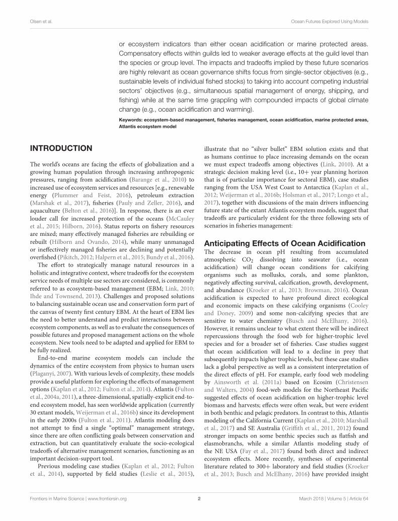
FIGURE 6 | Biomass response to 50-year scenarios with 0.5× fishing mortality on demersal fish. Panel explanations as in Figure 2.

stronger responses for individual functional groups or species(Figure 6B).

Increases in demersal fish groups were strongest in threeshallow or continental shelf systems: NE USA, Guam, andChesapeake Bay (Figure 6B). Indirect effects of decreased fishingon demersal fishes were minimal on lower trophic levels that arefound in demersal fish diets such as zooplankton and epibenthos.

Similar to the scenarios altering fishing for small pelagicfish or invertebrates, effects of reducing demersal fish harvestled to stronger responses than did increasing demersal fishharvest. For instance, completely removing fishing on thesegroups (Figure S8) led to stronger median responses (2% increasein sharks and 14% increase in demersal fish) and strongerresponses of particular functional groups (i.e., 95th percentileexhibiting increases of 5, 6, 46, and 117% for mammals, seabirds,sharks, and demersal fish, respectively). Also, in Figures S9–S15the additional results of the following six scenarios runs areshown: doubling fishing mortality on demersal fish (Figure S9),no fishing mortality for large pelagic fish (Figure S10), 0.5×fishing mortality for large pelagic fish (Figure S11), doublingfishing mortality for large pelagic fish (Figure S12), no fishingmortality for all groups (Figure S13), 0.5× fishingmortality for allgroups (Figure S14), and doubling fishingmortality for all groups(Figure S15).

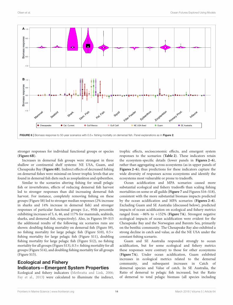
Ecological and FisheryIndicators—Emergent System PropertiesEcological and fishery indicators (Methratta and Link, 2006;Fay et al., 2013) were calculated to illuminate the indirect,

trophic effects, socioeconomic effects, and emergent systemresponses to the scenarios (Table 2). These indicators retainthe ecosystem-specific details (lower panels in Figures 2–6),rather than aggregating across ecosystems (as in upper panels ofFigures 2–6); thus predictions for these indicators capture thewide diversity of responses across ecosystems and identify theecosystems most vulnerable or prone to tradeoffs.

Ocean acidification and MPA scenarios caused moresubstantial ecological and fishery tradeoffs than scaling fishingmortalities on some or all guilds (Figure 7 and Figures S16–S18),consistent with the more substantial biomass impacts predictedby the ocean acidification and MPA scenarios (Figures 2–6).Excluding Guam and SE Australia (discussed below), predictedimpacts of ocean acidification on ecological and fishery metricsranged from −86% to +152% (Figure 7A). Strongest negativeecological impacts of ocean acidification were evident for theChesapeake Bay and the Norwegian and Barents Sea, primarilyon the benthic community. The Chesapeake Bay also exhibited astrong decline in catch and value, as did the NE USA under theconstant fishing scenario.

Guam and SE Australia responded strongly to oceanacidification, but for some ecological and fishery metricsthese responses were contrary to those for other ecosystems(Figure 7A). Under ocean acidification, Guam exhibitedincreases in ecological metrics related to the demersalcommunity, and subsequent increases in Catch ofdemersal species and Value of catch. In SE Australia, theRatio of demersal to pelagic fish increased, but the Ratioof demersal to total pelagic biomass (all species including






FIGURE 7 | Ecological and fishery indicators for scenarios. Metrics are generally ordered by: Ecological indicators (left), fishery indicators (right), pelagic (top), and

demersal (bottom). (A) Ocean acidification, via an additional 1% (day−1) mortality rate added for selected groups. Truncated values: Guam Dem/pelagic = 8.4; SE

Aus. Dyn Dem/pel fish = 6.4. (B) Spatial management closing 50% of continental shelf (<250m depth) to fishing. (C) Doubling fishing on small pelagic fish.

(D) Doubling fishing on invertebrates. (E) Halving fishing rates for demersal fish.

invertebrates) declined. Catch of demersal species thereforedeclined strongly in the SE Australia dynamic effort model asfishing fleets shifted to pelagic and benthopelagic stocks (in themodel with constant fishing rates, fleets change their species mixbut remain focused on demersals).

MPAs generally led to moderate increases in ecologicalmetrics related to demersal species, but stronger declines ineconomic metrics (Figure 7B). Shallow shelf systems werestrongly impacted by the MPA scenarios. For instance, underthe 50% MPA the NE USA model exhibited a large increase indemersal-fish biomass and declines inmetrics of catch, value, andexploitation rate. Similar declines in catch and fishery value wereevident for Chesapeake Bay (our shallowest system, with a full50% of model domain closed under this scenario). The Gulf ofCalifornia and Gulf of Mexico both exhibited large increases inpelagic and demersal catches, fishery value, and exploitation ratesunder the 50% MPA (Figure 7). This was due to stock recoveryin this scenario for these two systems. Additionally, in the Gulf ofMexicomenhaden (Brevoortia patronus, an abundant forage fish)experienced an increase in biomass.

Ecological indicators generally responded modestly to thefishing mortality scenarios, with stronger economic responsesfor metrics (e.g., value of catch, total catch, pelagic catch,demersal catch) directly reflecting impacts on fished species

and the importance of invertebrate fisheries in each ecosystem(Figures 7C–E and Figures S19–S30). For instance, doublingfishing on small pelagic fish led to a smaller than 10% changein most ecological indicators, with at most ∼22% declines inthe Ratio of pelagic biomass to primary production in the Gulfof Mexico (Figure 7C). Increased fishing on small pelagic fishgenerally led to increases in fishery metrics related to pelagiccatch and total value, except for the Chesapeake Bay andCalifornia Current. Similarly, doubling fishing on invertebrates(Figure 7D) led to little change in ecological metrics, but ledto increases in Catch of pelagic species (e.g., for squid in theCalifornia current), as well as for Catch of demersal species (crabsand lobsters in NE USA and Chesapeake Bay) and Value of catch(for instance driven by scallops and lobster in the NE USA andDungeness crab in the California Current). Halving fishing fordemersal species (Figure 7E) caused slight increases for mostsystems in Ratios of demersal to pelagic biomass or Ratios ofdemersal biomass to primary production. One exception wasfor the Gulf of Mexico, where these ratios declined slightly(this was due primarily to declines in a single demersal fishgroup (Deep Serranidae); most other demersal fish in this modelscenario increased in abundance or were stable). Halving fishingfor demersal species caused less than a 5% decline in most fisherymetrics (other than the direct metric of demersal fishery catch),






but with slightly stronger declines in fishery metrics for Guam(where total harvests and value are dominated by nearshore,demersal species).

DISCUSSION

Here, we build on previous efforts to compare marine ecosystems(Megrey et al., 2009c; Link et al., 2012) by applying a global setof ecosystem models that can predict the tradeoffs inherent tothree opportunities and challenges for EBM: ocean acidification,MPAs, and altering the mix of fishing effort across species. Themost striking result is that across these eight ecosystems theAtlantis ecosystem model projections suggest stronger impactsfrom ocean acidification and MPAs than from altering the mixof fishing effort, both in terms of guild-level biomass and interms of indicators of ecological and fishery structure. Eventhen, the vast majority of the impacts are moderate at thespecies or group level and dampened further at more aggregatedtaxonomic levels (guilds). This demonstrates the stability ofconsidering higher levels of hierarchy (Fogarty et al., 2012;Link et al., 2012). The opportunity to manage at the guildlevel, taking advantage of greater stability there, merits furtherconsideration. Biotic guilds are intriguing (Ross, 1986), as theyshow within guild compensation by component taxa in responseto a dynamic environment (Auster and Link, 2009). There isclearly greater stability in terms of biomass, and hence catch,at an aggregate level (Duplisea and Blanchard, 2005; Fogartyet al., 2012; Link et al., 2012). This “portfolio” effect (Schindleret al., 2015), when managed for, results in less variability incatches, greater economic value, and more regulatory, economicand biotic stability. Results here show similar patterns associatedwith aggregate stability. These results provide fresh and usefulinput to regional tradeoff analysis aimed at continuing fisheriesexploitation under increased ocean acidification. Proposingharvest policies, testing them, and managing at this aggregate orguild level (while still complying with single species mandates)through managing species complexes (Gaichas et al., 2017) orsetting ecosystem biomass caps (Link, 2018) undoubtedly meritsfurther exploration in inter-sectoral tradeoff analyses and isclearly supported as something that has observable benefits fromour results.

Ocean acidification effects simulated in the eight globalregions here led to indirect trophic effects, which often radiated toadditional species including predators; the effects were typicallynegative rather than positive, but occurred at the level ofparticular species (or functional groups). At the aggregated levelof guilds, compensatory effects led to average responses thatwere minimal. Our results are consistent with previous modeling(Kaplan et al., 2010; Griffith et al., 2011; Marshall et al., 2017) thatsuggests that if ocean acidification leads to direct mortality onbenthic invertebrates, indirect impacts will evolve on predatoryfish and dependent demersal fisheries. Divergence from this trendwas apparent, however, most notably for the NE USA, whereFay et al. (2017) predict strong impacts of ocean acidificationon benthic fish. Simulations for the NE USA here run counterto this, but illustrate a key uncertainty in our understanding of

direct ocean acidification effects. In Fay et al. (2017), depositfeeders (e.g., amphipods, isopods) are assumed to be directlyaffected by ocean acidification, while in our scenarios they arenot, and in fact increase by approximately 10–15%, leading to anincrease in forage available for predators such as demersal fish.This illustrates the need for improved, direct process studies ofocean acidification effects on all life stages of abundant foragespecies such as these deposit feeders, and also euphausiids (seeMcLaskey et al., 2016), as well as consistent application of suchstudies across ecosystem models.

Ecological tradeoffs inherent in MPAs (Fulton et al., 2015)evolved across our eight modeled ecosystems, but at the levelof individual species or groups (identifying “winning” speciesthat benefit and “losing” species that decline), rather than atthe more aggregated guild level. This is similar to the effects ofocean acidification, except that more “winners” were apparentin our MPA scenarios than OA scenarios. Additionally, becausewe simulated MPAs as closures to fishing of the continental shelf(e.g., 50% closure of area <250m depth), shallow systems weremore strongly impacted by these scenarios, as were systems forwhich the “base case” or status quo largely lacked spatial fisherymanagement. Overall, MPAs led to declines in most indicatorsof fishery yield and value, highlighting that in addition to trade-offs across species, there are trade-offs among ecological andeconomic considerations (Kaplan et al., 2012). Exceptions to thiswere for two systems (Gulf of Mexico and Gulf of California)that have high exploitation rates under base case conditions. Inthese systems, the relaxation of fishing pressure led to recoveryof particular species (but not necessarily entire ecological guilds)that led to long-term increases in catch and harvest value.

Our scenarios that altered fishing effort across species causedless drastic responses than did ocean acidification or MPAs;this was true in terms of biomass and also indicators of fishingand ecological response. The responses of birds, mammals,or sharks to these fishing scenarios were inconsistent acrosssystems, and the average responses (at the guild level) wereminimal. Furthermore, the exact mechanisms of change werehighly system dependent (e.g., SE Australia, Chesapeake Bay).Doubling or halving of existing fishing rates on all harvestedforage stocks (allowing other forage species to compensate insome cases) did not lead to strong impacts on predators in mostcases. Other global ecosystemmodeling efforts (Smith et al., 2011;Pikitch et al., 2014) as well as field observations (Cury et al.,2011; Bertrand et al., 2012; McClatchie et al., 2016) suggest thatcertain seabirds and marine mammals may be more vulnerableto the availability of forage stocks, particularly when we considerappropriate spatial scales of interaction (Sydeman et al., 2017).In contrast to this, a synthesis of USA fish, marine mammal, andbird populations has recently argued against this vulnerability formost predators (Hilborn et al., 2017). Within the context of thisdebate, our results suggest minimal guild-level impacts of foragedepletion, under three assumptions within the simulations: (1)fishing focuses only on a subset of (currently targeted) foragespecies and at most 2× baseline rates; (2) fisheries were notconcentrated near seabird and mammal breeding sites; and (3)models such as Atlantis include realistic age structure and densitydependence (Walters et al., 2016). However, the sensitivity of






individual species (or functional groups) in our models arguesfor future modeling at the species level (e.g., Punt et al., 2016),perhaps including spatial overlap and movement of mammals orbirds and forage (Boyd et al., 2014).

Increased fishing for invertebrates (including squid, shrimp,crabs, and shellfish) consistently led to higher catch and valuein most of our simulated ecosystems, with minimal effects onindicators of ecosystem structure. In contrast to this, Eddyet al. (2017) found that increasing fishery exploitation rates ofinvertebrates using a global suite of Ecopath with Ecosim (EwE)models had considerable ecosystem wide effects, though typicallythose increases in fishing rates and declines in invertebratebiomass were stronger than what we tested here. Our resultsfor fishing scenarios (particularly in Supporting Information)demonstrated that removal of fishing caused larger changes tothe ecosystem and fishery structure than did doubling of fishing.We hypothesize this is because many of these systems have longhistories of fishing with even higher fishing pressure than todayand are currently quite far from their original unfished states.Strong shifts in the ecosystem may occur at relatively low fishingrates (Samhouri et al., 2010). Overall, our results from the fishingscenarios suggest the necessity of cross-sectoral EBM: decisionsregarding fishing rates, effort, and catches can be overwhelmed bylarger multi-sector changes related to spatial management, andby the threat of global change.

Comparing the ecological and catch indicators gives insightsinto tradeoffs between socioeconomic effects of fishing (on thefishing industry and fishing communities) and ecological changesas seen in the response to various changes in fishing pressure.The indicators used were chosen based on studies that haveanalyzed their merits and usefulness (Fulton et al., 2005; Riceand Rochet, 2005; Methratta and Link, 2006; Shin and Shannon,2010), and although several are interdependent (e.g., “demersalcatch” and “fish catch” are subsets of “total catch”), they areincluded as they allow splitting the responses into meaningfulecological or fisheries sub-units. This can be seen from Figure 7A

where the strong decline in total catch for the NE USA Fixedand Chesapeake Bay was driven by the strong decline in demersalcatches while the pelagic catches remained closer to the base case.Similar interdependencies are present between the “Bio/PP,” “PelBio/PP,” and “Dem bio/PP,” between “Exp rate” and “Fish exprate,” and between the “MTL bio” and “MTL catch” indicators.Though these interdependencies can be easily interpreted, wecaution against visually “integrating” the area of the radar plots,and point readers to multivariate methodologies that distil suchindicator scores into independent axes, e.g. Ten Brink et al.(1991); Collie et al. (2003), and Coll et al. (2010). The strength andpresence of tradeoffs among indicators when analyzed visuallyusing radar plots may also be influenced by the ordering ofindicators around the axes of the plot (e.g., Shin et al., 2010).Ideally the set of indicators chosen to be presented in tradeoffplots should reflect the full set of management objectives; mostsensibly this selection and summary of indicators is probablyachieved in partnership with managers and stakeholders (Punt,2015). In part the lack of balance across our indicators reflectsdiffering levels of complexity in human components of the rangeof modeled ecosystems, and the need to compute a common set

of measures across ecosystems. Specific analysis of the radar plotsshowed that doubling fishing mortality on invertebrates gavethe most consistently positive results across models (Figure 7D),with no decreases in any of the catch indicators and withindicator values>150% in several models for Pelagic catch, Totalcatch, Exploitation rate, Value, and Demersal catch. None of theecological indicators showed a strong response (all were closeto 100%, e.g., equal to the base case) for any of the models.A similar, but less clear pattern could be seen for the scenariodoubling fishing mortality on small pelagics, but here the positiveresponses were not so apparent, and one model, the ChesapeakeBay responded negatively for several of the catch indicators.Again, all models had no responses (close to 100%, e.g., theywere equal to the base case) for the ecological indicators. Lastly,halving the fishing mortality on demersals gave little responseon either ecological or catch indicators. These results indicatethat the marine ecosystems modeled in this study are moreresilient and less affected by changes in fishing pressure thanare the fishing industry and fishing communities, and that themost positive effects may be achieved by increasing fishingpressure on invertebrates. However, it is worth inserting a noteof caution here. Invertebrates are typically represented as bulkbiomass pools in Atlantis (and other ecosystem-level models)and as such may not be capturing their ecological processes withsufficient nuance. Consequently, these findings should be takenas preliminary indicators only and more detailed case-specificconsideration should be given to any particular system lookingto significantly increase pressure on invertebrate stocks, so as toavoid unintended negative consequences (Eddy et al., 2017).

Our results give an indication of potential tradeoffs that needto be further evaluated and studied for each ecosystem separatelybefore being proposed as management action, but clearlyillustrate how ecosystem modeling can be used to highlight themost interesting management action among a suite of possiblealternatives. Specifically, our results indicate that any fisheriesmanagement or area-based protection measures to be consideredfirst have to take into consideration the effects of OA, as theeffects of OA greatly overwhelm effects of managing humanactivities. Since OA has its greatest effect on the epibenthosguild, it can be hypothesized that the combined effect of OAand any increase in fisheries targeting epibenthic organism (e.g.,molluscs or crustaceans) would lead to aggregated impact onthe epibenthic guild. Thus, management actions that are takenwithout considering the effects of OA may have unforeseen oreven detrimental effects. By running combination scenarios OAwith fisheries management and marine protection more definiteadvice on the potential trade-offs can be elucidated.

There is value in a comparative approach (Megrey et al.,2009b; Murawski et al., 2010) and in using common indicators(Shin et al., 2010). Marine ecosystems are complex, andunderstanding their fundamental processes, functioning,dynamics, and structures is often challenging. Monitoringand experimentation are essential, but logistically difficult atappropriate scales and extremely limited for many regions.Comparison of modeled ecosystems facilitates learning andunderstanding about marine ecosystems in that commonscenarios, tested across a range of ecosystem types, can confirm or






elicit common responses and highlight distinctions. A commonindicator set facilitates comparison, helps researchers elucidateunderstanding of marine ecosystems, and highlights commonproblem areas in terms of modeling skill, understanding, ormajor pressures. Common scenarios also provide the communityof practitioners a set of standards to consistently interpret statusof ecosystems, results of forecasts, and relative importance ofresponses to common scenarios and pressures. The debate overindicator selection (Rice and Rochet, 2005; Shin et al., 2010)seems to be settling in this community of practice, with a suiteof indicators similar to those presented here typically emerging.The next challenge is to convert a common set of indicators intothresholds or control rules (Link, 2005; Samhouri et al., 2010;Large et al., 2015; Tam et al., 2017) that can be tested acrossecosystems to inform decision-makers when action is neededand what level of action would be appropriate.

Caveats and Next StepsWhile common patterns are evident across many of the modeledsystems, it is appropriate to say that this may be because asingle modeling framework was used. While the models were ofdifferent ecosystem types and of radically different spatial extents,they were all implemented within a single framework, Atlantis.Interpretation of the results requires caution and preferablywith broader validation or verification of the general patterns ofoutcomes. While cross-ecosystem comparisons (Murawski et al.,2010) (within a common modeling approach) can provide someinsight into responses to future scenarios for management andocean change, a complementary approach is to apply multi-model comparison (Gårdmark et al., 2013; Townsend et al., 2014;Ianelli et al., 2016). Considering multiple model frameworkswith distinct underlying structural assumptions can quantify howdecisions about taxonomic aggregation and ecological and fisheryparameterization influence the strength of model response toperturbations (Pinnegar et al., 2005; Walters et al., 2016). Findingcommon patterns in the results of such ensembles gives moreconfidence in the general robustness of those findings and thusovercomes uncertainties due to model choice.

The current results examine the effects of each of the threedrivers separately. In reality these interact and the presentanalysis should be expanded to run scenarios combiningincreasing OA with marine protection and changes in fisheries.However, the number of scenarios to run would increasedramatically and were unfortunately outside the scope andcapacity of the present experiment.

In interpreting these results, it is important to acknowledgethe specific limitations of the fishing and fishery managementscenarios implemented (Fulton et al., 2011), the lack ofdownscaled oceanographic projections informed by global earthsystem models (e.g., Marshall et al., 2017) in most regions,and the need for consideration of interactions between oceanacidification, ocean warming, range shifts, and other aspects ofglobal change (Griffith et al., 2012; Fernandes et al., 2017; Ihdeand Townsend, 2017). While more dynamic representations ofocean acidification are possible using Atlantis (Marshall et al.,2017), this degree of complication was beyond available resourcesfor some model locations. Similarly, the implementation of

fishing fleet effort dynamics required to explore some of themore nuanced responses to spatial management requires alevel of resources and information not available for all themodel locations. Consequently, our scenarios for MPAs weresimple, closing large areas to fishing but without displacementof fishing effort (Agardy et al., 2011); more detailed modelingof spatial fleet dynamics has been undertaken in only someAtlantis applications (e.g., NE USA, SE Australia, also Girardinet al., 2017). More realistic MPA scenario modeling is neededto evaluate the effects of population spill overs from closures,fishing effort reallocation, as well as to elucidate the trade-offs between biodiversity protection and loss of economicallyvaluable fishing grounds. Our fishing scenarios are alsocrude adjustments of fishing mortalities for small pelagicfish, invertebrates, and demersal fish; fully envisioning futurescenarios for fisheries has been considered at a global scale(Delgado et al., 2003; Merino et al., 2012) but should betranslated to each region given the local fishery and economiccontext.

Sensitivity testing of key parameters determining theperformance of the scenarios would have added betterunderstanding of how dependent scenario results are onparameter settings. However, due to the long run times ofthe models, such sensitivity analyses were not feasible tocarry out.

Our global analysis identifies some potential options andissues that need more in-depth and careful exploration usingregional models and more specific methods. Full EBM trade-off analysis should also encompass all human uses of marineecosystem to address multi-stakeholder perspectives. Moreover,the current Atlantis models take no account for cross bordermanagement issues (many are only located in a singleEEZ) which in practical real-world management are one ofthe most difficult issues to resolve in achieving holisticallysustainable EBM.

CONCLUSION

Our applications of the Atlantis end-to-end ecosystem modelevaluate how different trends in the future ocean conditionsmay lead to key tradeoffs among species, management actions,and societal choices. Evaluating tradeoffs is a pillar of EBM, andour results here underscore a point from Link (2010): fisheriesmanagement can negotiate allocation of harvest among stocksand sectors but must exist within the reality of “non-negotiable”limits set by ecosystem productivity. Our results suggest thateven if overall, aggregated levels of productivity and biomass arerelatively stable in the near future, as simulated here, scenarios forocean acidification can sharply decrease the productive capacityof individual species and functional groups, thus limiting thepotential tradeoff options for fisheries and marine conservation.While acknowledging that the use of zoning for fisheries andconservation may lead to some benefits (Fulton et al., 2014),it must also be acknowledged that (as shown here) closingareas for fishing as part of implementing marine protectionhas negative impacts on fisheries and the socioeconomics of






the fishing sector. Marine protected areas (whether driven byfishery management or multi-sector considerations such asenergy extraction and species conservation) similarly shift thespatial pattern of productivity by altering fishing mortality onparticular groups. Altering fishing effort has greater effect onthe socioeconomics of the fishing sector than on the ecosystem,indicating a resilience in the ecosystems modeled here to changesin fisheries management (which could in part be because thesesystems are already amongst some of the best managed globallyso they are starting from a good position). The challenge ofthe future will be to carry out inter-sectoral tradeoff analysesthat devise, test, and implement EBM strategies that detect andcope with these productivity shifts in the future and help tomaintain this ecosystem resilience. A possible future scenariowould be to explore whether a combination of increased OAand marine protection could have synergistic effects on thefisheries in terms of reduced catches and value of catch, orif indirect pathways would alleviate the socioeconomic effects.End-to-end models such as Atlantis can serve as strategic toolsto identify vulnerable species and fisheries within particularecosystems and serve as an important foundation for EBMtradeoff analyses. Our analysis using a suite of models spanningthe Pacific and Atlantic, both hemispheres and ranging fromthe Arctic to the tropics has shown that these can serve astestbeds to illuminate adaptive management strategies (Fulton,2010; Punt et al., 2014) that address multi-sector trade-offsthat are robust to the coming climate-driven shifts in marineecosystems.

AUTHOR CONTRIBUTIONS

Conceived and designed the experiments: EO, JL, IK, SG, GF.Performed the experiments: IK, HM-L, EO, EF, MW, TI, CA,CE, RoG, GF,MS-R. Analyzed the data: IK. Contributed reagents,materials, and analysis tools: EF, IK, HM-L, KJ, EO, GF, HT, MW.Interpreted Results: IK, EO, CA, JL, SG, RaG. Wrote the paper:IK, KJ, HM-L, EO, EF, SG, GF, CE, RoG, TI, MW. Designed themodel software used in analysis: EF.

ACKNOWLEDGMENTS

This publication was an outcome of the first InternationalAtlantis EcosystemModeling Summit (http://atlantis.cmar.csiro.au/; http://www/en/atlantis/Atlantis-Summit.html) which tookplace in Honolulu, Hawaii on December 7–11, 2015 and wasconvened and funded by CSIRO (Australia), NOAA Fisheries(US), and IMR (Norway) and the Norwegian Research Council.EO and CE received funding from the Norwegian ResearchFund project PRIME TRADEOFFS (Cofasp ID 1277). HM-L was funded through the grant “Implementing Ecosystem-Based Fisheries Management: Two Case Studies in the NorthernGulf of California” from The David and Lucile PackardFoundation to CEDO Intercultural, and a Microsoft AzureResearch Award “Exploring ecosystem-level effects of fisheries,management, and climate change in marine systems” providedcloud computing resources. KJ was funded in part by agrant from Washington Sea Grant, University of Washington,pursuant to National Oceanic and Atmospheric AdministrationAward No. NA15OAR4170181. GF was funded in part by agrant from the Cooperative Institute for the North AtlanticRegion, Woods Hole Oceanographic Institution, pursuant toNational Oceanic and Atmospheric Administration AwardNo. NA14OAR4320158. IK and California Current modeldevelopment benefited greatly from a grant from the NOAAOcean Acidification Program and National Centers for CoastalOcean Science. MW and the Guam model development wasfunded by the NOAA Coral Reef Conservation Program. Theviews expressed herein are those of the author(s) and do notnecessarily reflect the views of NOAA or any of its sub-agencies.We thank Dr. Kristin Marshall for comments on a draft of thismanuscript.

SUPPLEMENTARY MATERIAL

The Supplementary Material for this article can be foundonline at: https://www.frontiersin.org/articles/10.3389/fmars.2018.00064/full#supplementary-material

REFERENCES

Agardy, T., di Sciara, G. N., and Christie, P. (2011). Mind the gap: addressingthe shortcomings of marine protected areas through large scale marinespatial planning. Mar. Policy 35, 226–232. doi: 10.1016/j.marpol.2010.10.006

Ainsworth, C. H., Samhouri, J. F., Busch, D. S., Cheung, W. W. L., Dunne, J.,and Okey, T. A. (2011a). Potential impacts of climate change on NortheastPacific marine foodwebs and fisheries. ICES J. Mar. Sci. 68, 1217–1229.doi: 10.1093/icesjms/fsr043

Ainsworth, C. H., Schirripa, M. J., and Morzaria-Luna, H. (2015). An Atlantis

Ecosystem Model for the Gulf of Mexico Supporting Integrated Ecosystem

Assessment. Miami, FL: NOAA. NFMS. SFSC.Ainsworth, C., Kaplan, I. C., Levin, P. S., Cudney-Bueno, R., Fulton, E. A.,

Mangel, M., et al. (2011b). Atlantis Model Development for the Northern Gulf of

California. Seattle, WA: NOAA Technical Memorandum NMFS-NWFSC-110.Auster, P. J., and Link, J. S. (2009). Compensation and recovery of feeding guilds in

a northwest Atlantic shelf fish community. Mar. Ecol. Prog. Ser. 382, 163–172.doi: 10.3354/meps07962

Barange, M., Field, J. G., Harris, R. P., Hoffmann, E. E., Perry, R. I., and Werner,F. (2010). Marine Ecosystems and Global Change. Oxford: Oxford UniversityPress.

Belton, B., Bush, S. R., and Little, D. C. (2016). Aquaculture: are farmed fish justfor the wealthy? Nature 538:171. doi: 10.1038/538171d

Bertrand, S., Joo, R., Arbulu Smet, C., Tremblay, Y., Barbraud, C., andWeimerskirch, H. (2012). Local depletion by a fishery can affect seabirdforaging. J. Appl. Ecol. 49, 1168–1177. doi: 10.1111/j.1365-2664.2012.02190.x

Boyd, C., Punt, A. E., Weimerskirch, H., and Bertrand, S. (2014). Movementmodels provide insights into variation in the foraging effort of central placeforagers. Ecol. Modell. 286, 13–25. doi: 10.1016/j.ecolmodel.2014.03.015

Browman, H. I. (2016). Applying organized scepticism to ocean acidificationresearch. ICES J. Mar. Sci. 73, 529–536. doi: 10.1093/icesjms/fsw010

Bundy, A., Bohaboy, E. C., Hjermann, D. Ø., Mueter, F. J., Fu, C., and Link, J. S.(2012). Common patterns, common drivers: comparative analysis of aggregatesurplus production across ecosystems. Mar. Ecol. Prog. Ser. 459, 203–218.doi: 10.3354/meps09787

Bundy, A., Chuenpagdee, R., Boldt, J. L., de Fatima Borges, M., Camara, M.L., Coll, M., et al. (2016). Strong fisheries management and governance


http://atlantis.cmar.csiro.au/

http://atlantis.cmar.csiro.au/

http://www/en/atlantis/Atlantis-Summit.html

https://www.frontiersin.org/articles/10.3389/fmars.2018.00064/full#supplementary-material

https://doi.org/10.1016/j.marpol.2010.10.006

https://doi.org/10.1093/icesjms/fsr043

https://doi.org/10.3354/meps07962

https://doi.org/10.1038/538171d

https://doi.org/10.1111/j.1365-2664.2012.02190.x

https://doi.org/10.1016/j.ecolmodel.2014.03.015

https://doi.org/10.1093/icesjms/fsw010






positively impact ecosystem status. Fish Fish. 18, 412–439. doi: 10.1111/faf.12184

Busch, D. S., and McElhany, P. (2016). Estimates of the direct effect of seawater phon the survival rate of species groups in the California current ecosystem. PLoSONE 11:e0160669. doi: 10.1371/journal.pone.0160669

Christensen, V., and Walters, C. J. (2004). Ecopath with Ecosim:methods, capabilities and limitations. Ecol. Modell. 172, 109–139.doi: 10.1016/j.ecolmodel.2003.09.003

Cinti, A., Shaw, W., Cudney-Bueno, R., and Rojo, M. (2010). The unintendedconsequences of formal fisheries policies: social disparities and resourceoveruse in a major fishing community in the Gulf of California, Mexico. Mar.

Policy 34, 328–339 doi: 10.1016/j.marpol.2009.08.002Coll, M., Shannon, L. J., Yemane, D., Link, J. S., Ojaveer, H., Neira, S., et al. (2010).

Ranking the ecological relative status of exploited marine ecosystems. ICES J.

Mar. Sci. 67, 769–786. doi: 10.1093/icesjms/fsp261Collie, J. S., Gislason, H., and Vinther, M. (2003). Using AMOEBAs to display

multispecies, multifleet fisheries advice. ICES J. Mar. Sci. 60, 709–720doi: 10.1016/S1054-3139(03)00042-0

Cooley, S. R., and Doney, S. C. (2009). Anticipating ocean acidification’seconomic consequences for commercial fisheries. Environ. Res. Lett. 4:024007.doi: 10.1088/1748-9326/4/2/024007

Cury, P. M., Boyd, I. L., Bonhommeau, S., Anker-Nilssen, T., Crawford, R. J. M.,Furness, R. W., et al. (2011). Global seabird response to forage fish depletion–one-third for the birds. Science 334, 1703–1706. doi: 10.1126/science.1212928

Delgado, C. L., Wada, N., Rosegrant, M.W., Meijer, S., and Ahmed, M. (2003). Fishto 2020: Supply and Demand in Changing Global Markets. Penang: The WorldFish Center.

Drinkwater, K. F., Mueter, F., Friedland, K. D., Taylor, M., Hunt, G. L., Jr., Hare,J., et al. (2009). Recent climate forcing and physical oceanographic changesin northern hemisphere regions: a review and comparison of four marineecosystems. Prog. Oceanogr. 81, 10–28. doi: 10.1016/j.pocean.2009.04.003

Duplisea, D. E., and Blanchard, F. (2005). Relating species and communitydynamics in an heavily exploited marine fish community. Ecosystems 8,899–910. doi: 10.1007/s10021-005-0011-z

Eddy, T. D., Lotze, H. K., Fulton, E. A., Coll, M., Ainsworth, C. H., de Araújo, J.N., et al. (2017). Ecosystem effects of invertebrate fisheries. Fish Fish. 18, 40–53.doi: 10.1111/faf.12165

Fay, G., Large, S. I., Link, J. S., and Gamble, R. J. (2013). Testing systemicfishing responses with ecosystem indicators. Ecol. Modell. 265, 45–55.doi: 10.1016/j.ecolmodel.2013.05.016

Fay, G., Link, J. S., andHare, J. A. (2017). Assessing the effects of ocean acidificationin the Northeast US using an end-to-end marine ecosystem model. Ecol.Modell. 347, 1–10. doi: 10.1016/j.ecolmodel.2016.12.016

Fernandes, J. A., Papathanasopoulou, E., Hattam, C., Queirós, A. M., Cheung,W. W. W. L., Yool, A., et al. (2017). Estimating the ecological, economic andsocial impacts of ocean acidification and warming on UK fisheries. Fish Fish.

18, 389–411. doi: 10.1111/faf.12183Fogarty, M. J., Overholtz, W. J., and Link, J. S. (2012). Aggregate surplus

production models for demersal fishery resources of the Gulf of Maine. Mar.

Ecol. Prog. Ser. 459, 247–258. doi: 10.3354/meps09789Fu, C., Gaichas, S., Link, J. S., Bundy, A., Boldt, J. L., Cook, A. M., et al.

(2012). Relative importance of fisheries, trophodynamic and environmentaldrivers in a series of marine ecosystems. Mar. Ecol. Prog. Ser.. 459, 169–184.doi: 10.3354/meps09805

Fulton, E. A. (2001). The Effects Of Model Structure And Complexity On The

Behaviour And Performance Of Marine Ecosystem Models. Ph.D Thesis, Schoolof Zoology, University of Tasmania, Hobart, TAS.

Fulton, E. A. (2010). Approaches to end-to-end ecosystemmodels. J. Mar. Syst. 81,171–183. doi: 10.1016/j.jmarsys.2009.12.012

Fulton, E. A. (2011). Interesting times: Winners, losers, and system shiftsunder climate change around Australia. ICES J. Mar. Sci. 68, 1329–1342.doi: 10.1093/icesjms/fsr032

Fulton, E. A., Bax, N. J., Bustamante, R. H., Dambacher, J. M., Dichmont, C.,Dunstan, P. K., et al. (2015). Modelling marine protected areas: insights andhurdles. Philos. Trans. R. Soc. Lond. B Biol. Sci. 370. doi: 10.1098/rstb.2014.0278

Fulton, E. A., Link, J. S., Kaplan, I. C., Savina-Rolland, M., Johnson, P.,Ainsworth, C., et al. (2011). Lessons in modelling and management

of marine ecosystems: the Atlantis experience. Fish Fish. 12, 171–188.doi: 10.1111/j.1467-2979.2011.00412.x

Fulton, E. A., Parslow, J. S., Smith, A. D. M., and Johnson, C. R.(2004a). Biogeochemical marine ecosystem models. 2. The effect ofphysiological data on model performance. Ecol. Modell. 173, 371–406.doi: 10.1016/j.ecolmodel.2003.09.024

Fulton, E. A., Smith, A. D. M., and Johnson, C. R. (2004b). Biogeochemical marineecosystem models I: IGBEM - a model of marine bay ecosystems. Ecol. Modell.

174, 267–307. doi: 10.1016/j.ecolmodel.2003.09.027Fulton, E. A., Smith, A. D. M., Smith, D. C., and Johnson, P. (2014). An

integrated approach is needed for ecosystem based fisheries management:insights from ecosystem-level management strategy evaluation. PLoS ONE

9:e84242. doi: 10.1371/journal.pone.0084242Fulton, E. A., Smith, A., and Punt, A. E. (2005). Which ecological indicators

can robustly detect effects of fishing? ICES J. Mar. Sci. 62, 540–551.doi: 10.1016/j.icesjms.2004.12.012

Gaichas, S. K., Fogarty, M., Fay, G., Gamble, R., Lucey, S., and Smith, L. (2017).Combining stock, multispecies, and ecosystem level fishery objectives withinan operational management procedure: simulations to start the conversation.ICES J. Mar. Sci. 74, 552–565. doi: 10.1093/icesjms/fsw119

Gaichas, S., Skaret, G., Falk-Petersen, J., Link, J. S., Overholtz, W., Megrey, B. A.,et al. (2009). A comparison of community and trophic structure in five marineecosystems based on energy budgets and system metrics. Prog. Oceanogr. 81,47–62. doi: 10.1016/j.pocean.2009.04.005

Garcia, S. M., Kolding, J., Rice, J., Rochet, M. J., Zhou, S., Arimoto, T., et al. (2012).Reconsidering the consequences of selective fisheries. Science 335, 1045–1047.doi: 10.1126/science.1214594

Gårdmark, A., Lindegren, M., Neuenfeldt, S., Blenckner, T., Heikinheimo, O.,Müller-Karulis, B., et al. (2013). Biological ensemble modeling to evaluatepotential futures of living marine resources. Ecol. Appl. 23, 742–754.doi: 10.1890/12-0267.1

Gill, D. A., Mascia, M. B., Ahmadia, G. N., Glew, L., Lester, S. E., Barnes, M., et al.(2017). Capacity shortfalls hinder the performance of marine protected areasglobally. Nature 543, 665–669. doi: 10.1038/nature21708

Girardin, R., Fulton, E. A., Lehuta, S., Rolland, M., Thébaud, O., Travers-Trolet, M., et al. (2017). Identification of the main processes underlyingecosystem functioning in the Eastern English Channel, with a focus onflatfish species, as revealed through the application of the Atlantis end-to-end model. Estuar. Coast. Shelf Sci. 201, 208–222. doi: 10.1016/j.ecss.2016.10.016

Griffith, G. P., Fulton, E. A., Gorton, R., and Richardson, A. J. (2012). Predictinginteractions among fishing, ocean warming, and ocean acidification in amarine system with whole-ecosystem models. Conserv. Biol. 26, 1145–1152.doi: 10.1111/j.1523-1739.2012.01937.x

Griffith, G. P., Fulton, E. A., and Richardson, A. J. (2011). Effects offishing and acidification-related benthic mortality on the southeastAustralian marine ecosystem. Glob. Chang. Biol. 17, 3058–3074.doi: 10.1111/j.1365-2486.2011.02453.x

Halpern, B. S., Frazier, M., Potapenko, J., Casey, K. S., Koenig, K., Longo, C., et al.(2015). Spatial and temporal changes in cumulative human impacts on theworld’s ocean. Nat. Comms. 6:7615 doi: 10.1038/ncomms8615

Halpern, B. S., Lester, S. E., and McLeod, K. L. (2010). Placing marine protectedareas onto the ecosystem-based management seascape. Proc. Nat. Acad. Sci.U.S.A. 107, 18312–18317. doi: 10.1073/pnas.0908503107

Hansen, C., Skern-Mauritzen, M., van der Meeren, G., Jähkel, A., and Drinkwater,K. (2016). Set-up of the Nordic and Barents Seas (NoBa) Atlantis Model.

Havforskningsinstituttet. Available online at: https://brage.bibsys.no/xmlui/handle/11250/2408609

Henriques, S., Pais, M. P., Vasconcelos, R. P., Murta, A., Azevedo, M.,Costa, M. J., et al. (2014). Structural and functional trends indicatefishing pressure on marine fish assemblages. J. Appl. Ecol. 51, 23–631.doi: 10.1111/1365-2664.12235

Hilborn, R. (2016). Policy: marine biodiversity needs more than protection.Nature535, 224–226. doi: 10.1038/535224a

Hilborn, R., Amoroso, R. O., Bogazzi, E., Jensen, O. P., Parma, A. M., Szuwalski,C., et al. (2017). When does fishing forage species affect their predators? Fish.Res. 191, 211–221. doi: 10.1016/j.fishres.2017.01.008


https://doi.org/10.1111/faf.12184

https://doi.org/10.1371/journal.pone.0160669


https://doi.org/10.1016/j.marpol.2009.08.002

https://doi.org/10.1093/icesjms/fsp261

https://doi.org/10.1016/S1054-3139(03)00042-0

https://doi.org/10.1088/1748-9326/4/2/024007

https://doi.org/10.1126/science.1212928

https://doi.org/10.1016/j.pocean.2009.04.003

https://doi.org/10.1007/s10021-005-0011-z







https://doi.org/10.1016/j.jmarsys.2009.12.012

https://doi.org/10.1093/icesjms/fsr032

https://doi.org/10.1098/rstb.2014.0278

https://doi.org/10.1111/j.1467-2979.2011.00412.x




https://doi.org/10.1016/j.icesjms.2004.12.012




https://doi.org/10.1890/12-0267.1

https://doi.org/10.1038/nature21708

https://doi.org/10.1016/j.ecss.2016.10.016

https://doi.org/10.1111/j.1523-1739.2012.01937.x

https://doi.org/10.1111/j.1365-2486.2011.02453.x

https://doi.org/10.1038/ncomms8615

https://doi.org/10.1073/pnas.0908503107

https://brage.bibsys.no/xmlui/handle/11250/2408609

https://brage.bibsys.no/xmlui/handle/11250/2408609

https://doi.org/10.1111/1365-2664.12235

https://doi.org/10.1038/535224a

https://doi.org/10.1016/j.fishres.2017.01.008





Hilborn, R., and Ovando, D. (2014). Reflections on the success oftraditional fisheries management. ICES J. Mar. Sci. 71, 1040–1046.doi: 10.1093/icesjms/fsu034

Hintze, J. L., and Nelson, R. D. (1998). Violin plots: a box plot-density tracesynergism. Am. Stat. 52, 181–184.

Holsman, K. K., Essington, T., Miller, T. J., Koen-Alonso, M., and Stockhausen, W.J. (2012). Comparative analysis of cod and herring production dynamics across13 northern hemisphere marine ecosystems.Mar. Ecol. Prog. Ser. 459, 231–246.doi: 10.3354/meps09765

Holsman, K., Samhouri, J., Cook, G., Hazen, E., Olsen, E., Dillard, M., et al.(2017). An ecosystem-based approach to marine risk assessment. Ecosyst.Health Sustain. 3:e01256. doi: 10.1002/ehs2.1256

Ianelli, J., Holsman, K. K., Punt, A. E., and Aydin, K. (2016).Multi-model inferencefor incorporating trophic and climate uncertainty into stock assessments. DeepSea Res. II Top. Stud. Oceanogr. 134, 379–389. doi: 10.1016/j.dsr2.2015.04.002

Ihde, T. F., Kaplan, I. C., Fulton, E. A., Gray, I. A., Hasan, M., Bruce, D.,et al. (2016). Design and Parameterization of the Chesapeake Bay Atlantis

Model: A Spatially Explicit End-to-End Ecosystem Model. NOAA TechnicalMemorandum NMFS-F/SPO-166, 145.

Ihde, T. F., and Townsend, H. M. (2017). Accounting for multiple stressorsinfluencing living marine resources in a complex estuarine ecosystem using anAtlantis model. Ecol. Modell. 365, 1–9. doi: 10.1016/j.ecolmodel.2017.09.010

Ihde, T., and Townsend, H. (2013). Interview with jason link: championfor ecosystem science and management. Fisheries 38, 363–369.doi: 10.1080/03632415.2013.813487

Jacobsen, N. S., Gislason, H., and Andersen, K. H. (2014). The consequencesof balanced harvesting of fish communities. Proc. Biol. Sci. 281:20132701.doi: 10.1098/rspb.2013.2701

Jähkel, A. (2013). Tuning the Diet of North-East Arctic Cod in the Barents Sea - An

Exploration with the end-to-end Model ATLANTIS. Available online at: http://hdl.handle.net/1956/7194

Kaiser, M. J., Clarke, K. R., Hinz, H., Austen, M., Somerfield, P. J., and Karakassis,I. (2006). Global analysis of response and recovery of benthic biota to fishing.Mar. Ecol. Prog. Ser. 311, 1–14. doi: 10.3354/meps311001

Kaplan, I. C., Horne, P. J., and Levin, P. S. (2012). Screening California currentfishery management scenarios using the Atlantis end-to-end ecosystem model.Prog. Oceanogr. 102, 5–18. doi: 10.1016/j.pocean.2012.03.009

Kaplan, I. C., Levin, P. S., Burden, M., and Fulton, E. A. (2010). Fishing catchshares in the face of global change: a framework for integrating cumulativeimpacts and single species management. Can. J. Fish. Aquat. Sci. 67, 1968–1982.doi: 10.1139/F10-118

Karnauskas, M., Kelble, C. R., Regan, S., Quenée, C., Allee, R., Jepson, M., et al.(2017). Ecosystem Status Report Update for the Gulf of Mexico. NOAATechnicalMemorandum NMFS-SEFSC-706.

Kjesbu, O. S., Bogstad, B., Devine, J. A., Gjøsæter, H., Howell, D., Ingvaldsen,R. B., et al. (2014). Synergies between climate and management for Atlanticcod fisheries at high latitudes. Proc. Natl. Acad. Sci. U.S.A. 111, 3487–3483.doi: 10.1073/pnas.1316342111

Kroeker, K. J., Kordas, R. L., Crim, R., Hendriks, I. E., Ramajo, L., Singh, G. S.,et al. (2013). Impacts of ocean acidification on marine organisms: quantifyingsensitivities and interaction with warming. Glob. Chang. Biol. 19, 1884–1896.doi: 10.1111/gcb.12179

Large, S. I., Fay, G., Friedland, K. D., and Link, J. S. (2015). Critical points inecosystem responses to fishing and environmental pressures. Mar. Ecol. Prog.

Ser. 521, 1–17. doi: 10.3354/meps11165Leslie, H., Sievanen, L., Crawford, T. G., Gruby, R., Villanueva-Aznar, H. C.,

and Campbell, L. M. (2015). Learning from ecosystem-based management inpractice. Coast. Manag. 43, 471–497. doi: 10.1080/08920753.2015.1051424

Lester, S. E., Halpern, B. S., Grorud-Colvert, K., Lubchenco, J., Ruttenberg, B. I.,Gaines, S. D., et al. (2009). Biological effects within no-take marine reserves: aglobal synthesis.Mar. Ecol. Prog. Ser. 384, 33–46. doi: 10.3354/meps08029

Link, J. (2005). Translating ecosystem indicators into decision criteria. ICES J. Mar.

Sci. 62, 569–576. doi: 10.1016/j.icesjms.2004.12.015Link, J. (2010). Ecosystem-Based Fisheries Management: Confronting Tradeoffs.

Cambridge: Cambridge University Press. doi: 10.1017/CBO9780511667091Link, J. S. (2018). System-level optimal yield: increased value, less risk,

improved stability, and better fisheries. Can. J. Fish. Aquat. Sci. 75, 1–16.doi: 10.1139/cjfas-2017-0250

Link, J. S., Bundy, A., Overholtz, W. J., Shackell, N., Manderson, J.,Duplisea, D., et al. (2011). Ecosystem-based fisheries management in thenorthwest atlantic. Fish Fish. 12, 152–170. doi: 10.1111/j.1467-2979.2011.00411.x

Link, J. S., Fulton, E. A., and Gamble, R. J. (2010). The northeast US applicationof ATLANTIS: A full system model exploring marine ecosystem dynamics ina living marine resource management context. Prog. Oceanogr. 87, 214–234.doi: 10.1016/j.pocean.2010.09.020

Link, J. S., Gaichas, S., Miller, T. J., Essington, T., Bundy, A., Boldt, J., et al.(2012). Synthesizing lessons learned from comparing fisheries production in 13northern hemisphere ecosystems: emergent fundamental features. Mar. Ecol.

Prog. Ser. 459, 293–302. doi: 10.3354/meps09829Link, J. S., Stockhausen, W. T., Skaret, G., Overholtz, W., Megrey, B. A.,

Gjøsæter, H., et al. (2009). A comparison of biological trends from four marineecosystems: Synchronies, differences, and commonalities. Prog. Oceanogr. 81,29–46. doi: 10.1016/j.pocean.2009.04.004

Longo, C. S., Frazier, M., Doney, S. C., Rheuban, J. E., Macy, J., and Halpern,B. S. (2017). Using the ocean health index to identify opportunities andchallenges to improving southern ocean ecosystem health. Front. Mar. Sci. 4:20.doi: 10.3389/fmars.2017.00020

Marshak, A. R., Link, J. S., Shuford, R., Monaco, M. E., Johannesen, E.,Bianchi, G., et al. (2017). International perceptions of an integrated, multi-sectoral, ecosystem approach to management. ICES J. Mar. Sci. 74, 414–420.doi: 10.1093/icesjms/fsw214

Marshall, K. N., Kaplan, I. C., Hodgson, E. E., Hermann, A., Busch, D. S.,McElhany, P., et al. (2017). Risks of ocean acidification in the California currentfood web and fisheries: ecosystem model projections. Glob. Chang. Biol. 23,1525–1539. doi: 10.1111/gcb.13594

May, R. M., Beddington, J. R., Clark, C. W., Holt, S. J., and Laws, R.M. (1979). Management of multispecies fisheries. Science 205, 267–277.doi: 10.1126/science.205.4403.267

McCauley, D. J., Pinsky, M. L., Palumbi, S. R., Estes, J. A., Joyce, F. H., andWarner,R. R. (2015). Marine defaunation: animal loss in the global ocean. Science347:1255641. doi: 10.1126/science.1255641

McClatchie, S., Field, J., Thompson, A. R., Gerrodette, T., Lowry, M., Fiedler,P. C., et al. (2016). Food limitation of sea lion pups and the declineof forage off central and southern California. Open Science 3:150628.doi: 10.1098/rsos.150628

McLaskey, A. K., Keister, J. E., McElhany, P., Brady Olson, M., Shallin Busch, D.,Maher, M., et al. (2016). Development of Euphausia pacifica (krill) larvae isimpaired under pCO2 levels currently observed in the Northeast Pacific. Mar.

Ecol. Prog. Ser. 555, 65–78. doi: 10.3354/meps11839Megrey, B. A., Hare, J. A., Stockhausen, W. T., Dommasnes, A., Gjøsæter,

H., Overholtz, W., et al. (2009a). A cross-ecosystem comparison of spatialand temporal patterns of covariation in the recruitment of functionallyanalogous fish stocks. Prog. Oceanogr. 81, 63–92. doi: 10.1016/j.pocean.2009.04.006

Megrey, B. A., Link, J. S., Hunt, G. L., Jr., and Moksness, E. (2009c).Comparative marine ecosystem analysis: applications, opportunities,and lessons learned. Prog. Oceanogr. 81, 2–9. doi: 10.1016/j.pocean.2009.04.002

Megrey, B. A., Link, J. S., and Moksness, E. (2009b). Comparative marineecosystem structure and function: descriptors and characteristics. Prog.

Oceanogr. 81, 1–236. doi: 10.1016/j.pocean.2009.04.001Merino, G., Barange, M., Blanchard, J. L., Harle, J., Holmes, R., Allen, I., et al.

(2012). Canmarine fisheries and aquaculture meet fish demand from a growinghuman population in a changing climate? Glob. Environ. Change 22, 795–806.doi: 10.1016/j.gloenvcha.2012.03.003

Methratta, E., and Link, J. (2006). Evaluation of quantitative indicators for marinefish communities. Ecol. Indic. 6, 575–588. doi: 10.1016/j.ecolind.2005.08.022

Morzaria-Luna, H. N., Ainsworth, C. H., Kaplan, I. C., Levin, P. S., andFulton, E. A. (2013). Indirect effects of conservation policies on the coupledhuman-natural ecosystem of the Gulf of California. PLoS ONE 8:e64085.doi: 10.1371/journal.pone.0064085

Mueter, F. J., Broms, C., Drinkwater, K. F., Friedland, K. D., Hare, J. A., Hunt, G.L., Jr., et al. (2009). Ecosystem responses to recent oceanographic variabilityin high-latitude Northern Hemisphere ecosystems. Prog. Oceanogr. 81, 93–110.doi: 10.1016/j.pocean.2009.04.018


https://doi.org/10.1093/icesjms/fsu034


https://doi.org/10.1002/ehs2.1256

https://doi.org/10.1016/j.dsr2.2015.04.002


https://doi.org/10.1080/03632415.2013.813487

https://doi.org/10.1098/rspb.2013.2701

http://hdl.handle.net/1956/7194

http://hdl.handle.net/1956/7194



https://doi.org/10.1139/F10-118

https://doi.org/10.1073/pnas.1316342111

https://doi.org/10.1111/gcb.12179


https://doi.org/10.1080/08920753.2015.1051424



https://doi.org/10.1017/CBO9780511667091

https://doi.org/10.1139/cjfas-2017-0250

https://doi.org/10.1111/j.1467-2979.2011.00411.x






https://doi.org/10.1111/gcb.13594

https://doi.org/10.1126/science.205.4403.267


https://doi.org/10.1098/rsos.150628





https://doi.org/10.1016/j.gloenvcha.2012.03.003

https://doi.org/10.1016/j.ecolind.2005.08.022







Murawski, S. A., Steele, J. H., Taylor, P., Fogarty, M. J., Sissenwine, M. P., Ford,M., et al. (2010). Why compare marine ecosystems? ICES J. Mar. Sci. 67, 1–9.doi: 10.1093/icesjms/fsp221

Newell, R. I. E. (1988). “Ecological changes in Chesapeake Bay: are they the resultof overharvesting the eastern oyster, Crassostrea virginica?,” in Understanding

the Estuary. Advances in Chesapeake Bay Research, eds M. P. Lynch and E.C. Krome (Gloucester Point, VA: Chesapeake Research Consortium Publ 129),536–546.

Nyamweya, C., Sturludottir, E., Tomasson, T., Fulton, E. A., Taabu-Munyaho,A., Njiru, M., et al. (2016). Exploring Lake Victoria ecosystem functioningusing the Atlantis modeling framework. Environ. Modell. Softw. 86, 158–167.doi: 10.1016/j.envsoft.2016.09.019

Nye, J. A., Gamble, R. J., and Link, J. S. (2013). The relative impact ofwarming and removing top predators on the Northeast US large marinebiotic community. Ecol. Modell. 264, 157–168. doi: 10.1016/j.ecolmodel.2012.08.019

Ocean Conservancy, Cooley, S., Jewett, E., Reichert, J., Robbins, L., Shrestha,G., et al. (2015). Getting ocean acidification on decision makers’ to-dolists: dissecting the process through case studies. Oceanography 25, 198–211.doi: 10.5670/oceanog.2015.42

Orvik, K. A., and Skagset, Ø. (2005). Heat flux variations in the eastern NorwegianAtlantic current toward the Arctic from moored instruments, 1995-2005.Geophys. Res. Lett. 32:L14610. doi: 10.1029/2005GL023487

Páez-Osuna, F., Álvarez-Borrego, S., Ruiz-Fernández, A. C., García-Hernández, J.,Jara-Marini, M. E., Bergés-Tiznado, M. E., et al. (2017). Environmental statusof the Gulf of California: a pollution review. Earth Sci. Rev. 166, 181–205.doi: 10.1016/j.earscirev.2017.01.014

Patterson, H., Noriega, R., Georgeson, L., Larcombe, J., and Curtotti, R. (2017).Fishery Status Reports 2017, Australian Bureau of Agricultural and Resource

Economics and Sciences. Canberra, ACT: CC BY 4.0.Pauly, D., and Zeller, D. (2016). Catch reconstructions reveal that global marine

fisheries catches are higher than reported and declining. Nat. Commun.

7:10244. doi: 10.1038/ncomms10244Pikitch, E. K. (2012). The risks of overfishing. Science 338, 474–475.

doi: 10.1126/science.1229965Pikitch, E. K., Rountos, K. J., Essington, T. E., Santora, C., Pauly, D., Watson,

R., et al. (2014). The global contribution of forage fish to marine fisheries andecosystems. Fish Fish. 15, 43–64. doi: 10.1111/faf.12004

Pinnegar, J. K., Blanchard, J. L., Mackinson, S., Scott, R. D., and Duplisea,D. E. (2005). Aggregation and removal of weak-links in food-web models:system stability and recovery from disturbance. Ecol. Modell. 184, 229–248.doi: 10.1016/j.ecolmodel.2004.09.003

Plaganyi, E. E. (2007). Models for an Ecosystem Approach to Fisheries. Rome: FAO.Plummer, M. L., and Feist, B. E. (2016). Capturing energy from the

motion of the ocean in a crowded sea. Coast. Manage. 44, 464–485.doi: 10.1080/08920753.2016.1208877

Punt, A. E. (2015). Strategic management decision-making in a complex world:quantifying, understanding, and using trade-offs. ICES J. Mar. Sci. 74, 499–510.doi: 10.1093/icesjms/fsv193

Punt, A. E., Butterworth, D. S., deMoor, C. L., DeOliveira, J. A. A., andHaddon,M.(2014). Management strategy evaluation: best practices. Fish Fish. 17, 303–334.doi: 10.1111/faf.12104

Punt, A. E., MacCall, A. D., Essington, T. E., Francis, T. B., Hurtado-Ferro, F.,Johnson, K. F., et al. (2016). Exploring the implications of the harvest controlrule for Pacific sardine, accounting for predator dynamics: AMICEmodel. Ecol.Modell. 337, 79–95. doi: 10.1016/j.ecolmodel.2016.06.004

Rice, J. C., and Rochet, M.-J. (2005). A framework for selecting a suiteof indicators for fisheries management. ICES J. Mar. Sci. 62, 516–527.doi: 10.1016/j.icesjms.2005.01.003

Ross, S. T. (1986). Resource partitioning in fish assemblages: a review of fieldstudies. Copeia 1986, 352–388. doi: 10.2307/1444996

Samhouri, J. F., Levin, P. S., and Ainsworth, C. H. (2010). Identifyingthresholds for ecosystem-based management. PLoS ONE 5:e8907.doi: 10.1371/journal.pone.0008907

Savina, M., Condie, S. A., and Fulton, E. A. (2013). The role of pre-existing disturbances in the effect of marine reserves on coastal ecosystems:a modelling approach. PLoS ONE 8:e61207. doi: 10.1371/journal.pone.0061207

Schindler, D. E., Armstrong, J. B., and Reed, T. E. (2015). The portfolio concept inecology and evolution. Front. Ecol. Environ. 13, 257–263. doi: 10.1890/140275

Shin, Y. J., Bundy, A., Shannon, L. J., Simier,M., Coll, M., Fulton, E. A., et al. (2010).Can simple be useful and reliable? using ecological indicators to representand compare the states of marine ecosystems. ICES J. Mar. Sci. 67, 717–731.doi: 10.1093/icesjms/fsp287

Shin, Y.-J., and Shannon, L. J. (2010). Using indicators for evaluating, comparing,and communicating the ecological status of exploited marine ecosystems. 1.The IndiSeas project. ICES J. Mar. Sci. 67, 686–691. doi: 10.1093/icesjms/fsp273

Skern-Mauritzen, M., Ottersen, G., Handegard, N. O., Huse, G., Dingsør, G.E., Stenseth, N. C., et al. (2016). Ecosystem processes are rarely includedin tactical fisheries management. Fish Fish. 17, 165–175. doi: 10.1111/faf.12111

Smith, A. D. M., Brown, C. J., Bulman, C. M., Fulton, E. A., Johnson, P., Kaplan,I. C., et al. (2011). Impacts of fishing low-trophic level species on marineecosystems. Science 333, 1147–1150. doi: 10.1126/science.1209395

Smith, M. D., Fulton, E. A., and Day, R. W. (2015). Using an Atlantismodel of the southern Benguela to explore the response of ecosystemindicators for fisheries management. Environ. Modell. Softw. 69, 23–41.doi: 10.1016/j.envsoft.2015.03.002

Sydeman, W. J., Thompson, S. A., Anker-Nilssen, T., Arimitsu, M.,Bennison, A., Bertrand, S., et al. (2017). Best practices for assessingforage fish fisheries-seabird resource competition. Fish. Res. 194, 209–221.doi: 10.1016/j.fishres.2017.05.018

Tam, J. C., Link, J. S., Rossberg, A. G., Rogers, S. I., Levin, P. S., Rochet, M.-J.,et al. (2017). Towards ecosystem-based management: identifying operationalfood-web indicators for marine ecosystems. ICES J. Mar. Sci. 74, 2040–2052doi: 10.1093/icesjms/fsw230

Ten Brink, B. J. E., Hosper, S. H., and Colijn, F. (1991). A quantitative method fordescription and assessment of ecosystems: the Amoeba approach. Mar. Pollut.

Bull. 23, 265–270Townsend, H.M., Harvey, C., Aydin, K. Y., Gamble, R., Grüss, A., Levin, P. S., et al.

(2014). Report of the 3rd National Ecosystem Modeling Workshop (NEMoW 3):

Mingling Models for Marine Resource Management–Multiple Model Inference.NOAA Technical Memorandum NMFS-F/SPO-149.

van Denderen, P. D., Rijnsdorp, A. D., and van Kooten, T. (2016). Using marinereserves to manage impact of bottom trawl fisheries requires considerationof benthic food-web interactions. Ecol. Appl. 26, 2302–2310. doi: 10.1002/eap.1360

Voss, R., Quaas, M. F., Schmidt, J. O., Tahvonen, O., Lindegren, M.,and Möllmann, C. (2014). Assessing social–ecological trade-offs toadvance ecosystem-based fisheries management. PLoS ONE 9:e107811.doi: 10.1371/journal.pone.0107811

Walters, C., Christensen, V., Fulton, B., Smith, A. D. M., and Hilborn, R. (2016).Predictions from simple predator-prey theory about impacts of harvestingforage fishes. Ecol. Modell. 337, 272–280. doi: 10.1016/j.ecolmodel.2016.07.014

Walters, C., Christensen, V., Martell, S., and Kitchell, J. (2005). Possible ecosystemimpacts of applying MSY policies from single-species assessment. ICES J. Mar.

Sci. 62, 558–568. doi: 10.1016/j.icesjms.2004.12.005Walters, C., Pauly, D., and Christensen, V. (1999). Ecospace: prediction of

mesoscale spatial patterns in trophic relationships of exploited ecosystems, withemphasis on the impacts of marine protected areas. Ecosystems 2, 539–554.doi: 10.1007/s100219900101

Weigel, J.Y., Mannle, K. O., Bennett, N. J., Carter, E., Westlund, L., Burgener, V.,et al. (2014). Marine protected areas and fisheries: bridging the divide. Aquat.Conserv. 24, 199–215. doi: 10.1002/aqc.2514

Weijerman, M., Fulton, E. A., and Brainard, R. E. (2016a). Managementstrategy evaluation applied to coral reef ecosystems in support of ecosystem-based management. PLoS ONE 11:e0152577. doi: 10.1371/journal.pone.0152577

Weijerman, M., Fulton, E. A., Kaplan, I. C., Gorton, R., Leemans, R., Mooij,W. M., et al. (2015). An integrated coral reef ecosystem model to supportresource management under a changing climate. PLoS ONE 10:e0144165.doi: 10.1371/journal.pone.0144165

Weijerman,M., Kaplan, I. C., Fulton, E. A., Gorton, R., Grafeld, S., and Brainard, R.(2014).Design and Parameterization of a Coral Reef EcosystemModel for Guam.US Dep. Commer. NOAA Tech. Memo., NOAA-TM-NMFSPIFSC-43.



https://doi.org/10.1016/j.envsoft.2016.09.019


https://doi.org/10.5670/oceanog.2015.42

https://doi.org/10.1029/2005GL023487

https://doi.org/10.1016/j.earscirev.2017.01.014

https://doi.org/10.1038/ncomms10244




https://doi.org/10.1080/08920753.2016.1208877

https://doi.org/10.1093/icesjms/fsv193




https://doi.org/10.2307/1444996



https://doi.org/10.1890/140275





https://doi.org/10.1016/j.envsoft.2015.03.002

https://doi.org/10.1016/j.fishres.2017.05.018


https://doi.org/10.1002/eap.1360




https://doi.org/10.1007/s100219900101

https://doi.org/10.1002/aqc.2514







Weijerman, M., Link, J. S., Fulton, E. A., Olsen, E., Townsend, H., Gaichas, S.,et al. (2016b). Atlantis ecosystemmodel summit: report from a workshop. Ecol.Modell. 335, 35–38. doi: 10.1016/j.ecolmodel.2016.05.007

Wilberg, M., and Miller, T. (2010). Developing Spatially-Explicit Assessment Tools

for Eastern Oyster in Chesapeake Bay. Final Report. Technical Report no.TS-599-10 of the University of Maryland Center for Environmental Science.

Worm, B., Hilborn, R., Baum, J. K., Branch, T. A., Collie, J. S., Costello,C., et al. (2009). Rebuilding global fisheries. Science 325, 578–585.doi: 10.1126/science.1173146

Wu, L., Cai,W., Zhang, L., Nakamura, H., Timmermann, A., Joyce, T., et al. (2012).Enhanced warming over the global subtropical western boundary currents.Nat.Clim. Chang. 2, 161–166. doi: 10.1038/nclimate1353

Conflict of Interest Statement: The authors declare that the research wasconducted in the absence of any commercial or financial relationships that couldbe construed as a potential conflict of interest.

Copyright © 2018 Olsen, Kaplan, Ainsworth, Fay, Gaichas, Gamble, Girardin, Eide,

Ihde, Morzaria-Luna, Johnson, Savina-Rolland, Townsend, Weijerman, Fulton and

Link. This is an open-access article distributed under the terms of the Creative

Commons Attribution License (CC BY). The use, distribution or reproduction in

other forums is permitted, provided the original author(s) and the copyright owner

are credited and that the original publication in this journal is cited, in accordance

with accepted academic practice. No use, distribution or reproduction is permitted

which does not comply with these terms.




https://doi.org/10.1038/nclimate1353

http://creativecommons.org/licenses/by/4.0/








ocean futures under ocean acidification, marine …archimer.ifremer.fr/doc/00428/53948/55094.pdf ·...

Documents