Occupational Choices:

Economic Determinants of Land Invasions∗

F. Daniel Hidalgo†

Suresh Naidu

Simeon Nichter

Neal Richardson

April 30, 2007

Abstract

This study estimates the effect of economic conditions on redistributive conflict. Weexamine land invasions in Brazil using a panel dataset with over 50,000 municipality-year observations. Adverse economic shocks, instrumented by rainfall, cause the ruralpoor to invade and occupy large landholdings. This effect exhibits substantial hetero-geneity by land inequality and land tenure systems. In highly unequal municipalities,negative income shocks cause twice as many land invasions than in municipalities withaverage land inequality. We find no further evidence of heterogeneity on other observ-able variables. Cross-sectional regressions confirm the importance of land inequality inexplaining redistributive conflict.

Keywords: land conflict, inequality, redistribution, rainfall, political economy, devel-opment, social movement, collective actionJEL codes: D74, Q15, D3, O17, P16

∗The authors would like to thank Raymundo Nonato Borges, David Collier, Bernardo Mancano Fernan-des, Stephen Haber, Steven Helfand, Rodolfo Hoffmann, Ted Miguel, Bernardo Mueller, Jim Powell, DavidSamuels, Edelcio Vigna and participants in the Development Economics Seminar and the Latin AmericanPolitics Seminar at the University of California, Berkeley. A previous version of this paper was presented atthe XXVI International Congress of the Latin American Studies Association, San Juan, PR (March 15-18,2006). The authors recognize support of the National Science Foundation Graduate Research FellowshipProgram, the Jacob K. Javits Fellowship Program, and the UC Berkeley Center for Latin American Studies.

†Hidalgo, Nichter, and Richardson: Department of Political Science, University of California, Berke-ley; Naidu: Department of Economics, University of California, Berkeley. Authors’ email addresses:fdhidalgo@berkeley.edu; snaidu@econ.berkeley.edu; nichter@berkeley.edu; npr@berkeley.edu.

1

1 Introduction

Conflict over land is endemic to many rural economies. In environments marked by a highly

skewed distribution of property, incomplete land and credit markets, poorly or unevenly

enforced property rights, and weak political institutions, agents often resort to extralegal

means to improve their economic positions. The poor frequently invade private properties

and occupy them until either forcibly expelled or granted official titles. Land occupations

are prevalent in Brazil [CPT 1988-2004], South Africa [Simmons 2001], Venezuela [Econo-

mist 2001] and many other countries. How do economic conditions affect this redistributive

conflict?

This paper explores this question using a rich municipal-level dataset of 5,299 land

invasions from 1988 to 2004 in Brazil. Employing exogenous variation in income generated

by rainfall, this study finds that adverse economic shocks cause the rural poor to occupy

large landholdings. This effect is magnified by land inequality. In highly unequal munici-

palities, negative income shocks cause twice as many land invasions than in municipalities

with average land inequality. When using a measure of land polarization, which captures

the degree of bimodality of the land distribution, the effect is even stronger. Moreover,

cross-sectional specifications confirm the importance of land inequality in explaining redis-

tributive conflict.

In addition to heterogeneity by land inequality, we find that income shocks cause

significantly more land invasions in municipalities with a greater proportion of land under

fixed-rent contracts. We find no evidence of heterogeneity on other political and socioeco-

nomic variables. The impact of income shocks does not differ significantly across levels of

political competition, sharecropping, police expenditures, or social welfare spending. Our

findings provide new evidence on the underexplored relationship between inequality and

redistributive conflict.

2

While several papers have identified a causal relationship between income and con-

flict, none have found that this relationship varies by economic institutions or the distri-

bution of assets. Our paper is the first to show that the effect of income shocks exhibits

heterogeneity in ways consistent with qualitative evidence and economic theories of conflict.

Previous papers have been unable to examine many plausible sources of potential hetero-

geneity because of data limitations [Miguel, Satyanath, and Sergenti 2004; Do and Iyer

2006]. The rich nature of our data, however, allows us to test for a large set of interactions.

Importantly, the motivations behind the conflict we examine are explicitly redistributive,

while other work primarily considers civil wars, which are fought for a variety of economic

and non-economic reasons.

This paper also contributes to a longstanding debate in the fields of political science

and sociology: when do the rural poor become politically active? Studies of political change

have long explored this question because of the important historical role of agrarian class

conflict in institutional transitions [Moore 1966; Huntington 1968; Skocpol 1979; Luebbert

1991]. Much of this literature studies poverty, inequality and rural class conflict [e.g., Scott

1976; Popkin 1976], and some suggest that different systems of land tenure foster or inhibit

peasant mobilization. The theories, however, often point in contradictory directions. For

example, Stinchcombe [1961] and Paige [1975] argue that small landowners are typically

conservative, generally supporting modest reform movements, while Wolf [1969] claims that

they are more likely to be radicalized. The capacity for sharecroppers to mobilize is also

widely debated among these authors. These conclusions, however, are generally based on

in-depth case studies; few studies are quantitative1 and none attempt to identify the causal

impact of income shocks.

The paper is organized as follows. In Section 2, we present a brief overview of land

1But see Paige [1975] and Markoff [1996].

3

conflict in Brazil. Section 4 explains data sources. Our identification strategy is discussed

in Section 5. Section 6 presents basic results and robustness checks. Section 7 examines

heterogeneity across land inequality, land tenure, and other observable variables. Section 8

confirms the importance of land inequality in cross-municipality specifications, and Section

9 concludes.

2 Overall Context

According to the Food and Agricultural Organization of the United Nations, Brazil has

the eighth-most unequal distribution of land in the world [FAO 2005]. The concentration

of property in Brazil is so skewed that the largest 3.5 percent of landholdings represent

56 percent of total agricultural land. Land inequality has long persisted in Brazil.2 The

Gini coefficient of land inequality remained stable between 1967 and 1998, measuring 0.84

in both the beginning and end of the period. And while some regional differences exist,

with the North, Northeast and Center-West relatively more unequal than the South and

Southeast, land inequality in all regions is high when compared internationally [Hoffmann

1998; Griffin, Khan, and Ickowitz 2002].

Efforts to reduce Brazil’s land inequality have been hamstrung by political con-

straints. During the presidency of Getulio Vargas (1930-45), proposals for land reform

emerged but were quickly sidelined because Vargas relied on continued support from landed

elites [Morissawa 2001, p. 81]. In the early 1960s, President Joao Goulart initiated modest

land reform measures but was soon ousted by the military coup of 1964. Land reform stag-

nated during the twenty-year military dictatorship. Although President Castelo Branco

2High land inequality dates back to the initial European partitioning of the New World. During thecolonial period, the Portuguese monarchy divided Brazil’s territory into twelve captaincies. By bestowingthese massive properties to individuals, the Portuguese established a land structure based on latifundios,or large rural landholdings [Bethell 1987].

4

approved the Brazilian Land Statute (1964), which introduced the “social function” of

land as a legal concept and identified landholding categories eligible for expropriation, the

section relating to land reform was “virtually abandoned” due to immense pressure from

landed elites [Morissawa 2001, p. 99]. The authoritarian regime expropriated only eight

properties per year on average, and instead attempted to placate rural peasants through

colonization projects, which typically entailed resettlements to government land in the

Amazon [Alston, Libecap, and Mueller 1999, pp. 135-6].

Even since Brazil’s transition to democracy in 1985, land reform has been limited.

In 1985, President Jose Sarney launched the National Agrarian Reform Plan, which ambi-

tiously established a goal of resettling 1.4 million families during the following five years.

However, INCRA, the national agrarian reform agency, only resettled 90,000 families dur-

ing this period [Cardoso 1997, p. 24].3 Then, land reform virtually stopped during the

Collor de Mello presidency (1990-92). Afterwards, President Itamar Franco (1992-94) ini-

tiated an emergency land reform program aiming to redistribute land to 80,000 families,

but reached only 23,000 families [Cardoso 1997, p. 25].

Amidst limited formal land reform, many poor Brazilians have invaded private es-

tates and public lands, squatting in an attempt to appropriate land. As shown in Figure 1,

over 660,000 families—more than 3 million individuals—participated in land invasions in

the Brazilian countryside between 1988 and 2004 [CPT 2004]. By invading large landown-

ers’ property, poor Brazilians have placed the issue of land redistribution on the national

political agenda, pressuring the government to expropriate land. 4 Due in large part to

3INCRA is the Instituto Nacional de Colonizacao e Reforma Agraria (National Institute of Colonizationand Land Reform).

4In part due to such invasions, numerous surveys over the past twenty years reveal the overwhelmingpopularity of formal land reform in Brazil. For example, a 1987 survey found that 83 percent of respondentssupported “expropriating large properties that do not fulfill their social function” [Machado, Magri, andMasagcao 1986, p. 14]. More recently, a national IBOPE poll in 1998 found that 80 percent of respondentsfavored formal land reform.

5

these land invasions, land reform trebled under Fernando Henrique Cardoso (1995-2002),

reaching nearly 260,000 families during his presidency [INCRA 2005].

Land invasions (also termed “land occupations” in Brazil) are large undertakings,

each involving an average of 156 families. Because the land-poor face considerable obstacles

while invading land, coordination of their efforts is important. Consequently, many land

occupations are facilitated by social activists, who help to plan invasions and to assist

families while they squat on occupied properties. Activists affiliated with the Landless

Workers Movement (Movimento dos Trabalhadores Rurais Sem Terra – MST) or other

social groups identify rural properties that are most likely to be expropriated by the federal

government following an invasion, such as underutilized land that does not fulfill its “social

function” (de Janvry et al 1998: 15). Once a target property is identified, activists help

participants to gather food and materials for housing, arrange buses and cars, and develop

secret plans for invasions [Paiero and Damatto 1996, pp. 31-40](Ondetti 2002: 70).

Once a land invasion occurs, the immediate aftermath is extremely tense and fre-

quently violent. Landowners often seek to end invasions by both extralegal and legal

means, simultaneously firing bullets and filing charges. Violence is common—in 2003 alone,

55 land invaders were killed, 73 were physically attacked, and 155 received death threats

[CPT 2003]. To eject squatters, landowners often hire private militias, and may also ob-

tain expulsion orders from local judges enforceable by the military police (de Janvry et al

1998: 16). If the land invaders manage to remain on the property, the national land reform

agency (INCRA) may recognize their claim if it deems the occupied land is “nonproduc-

tive.”5 Given a complicated legal framework, the various legal proceedings involved in a

5If the national land reform agency (INCRA) determines that the occupied land is “productive,” then noexpropriation is legally possible. Otherwise, INCRA may recognize the land invaders’ claim by estimatingthe value of the land and offering a sum to the owner in exchange for expropriation. In some cases,government officials bargain with participants, offering property on government-owned land in exchange fordismantling camps (Ondetti 2002: 71).

6

land occupation take between six months and six years before land is officially expropriated

on behalf of squatters[Wolford 2001]. According to 1996 survey of all registered occupants

of invaded land, 57 percent had begun the official procedures to acquire a land title, while

only 5.6 percent had actually received it (Viero Schmidt et al 1998: 122). With their ex-

tensive experience in pressuring the government to expropriate land, social activists such

as those within the MST help participants to negotiate with the government and navigate

the legal system [Medeiros 2003, p. 52].6

Given the challenges involved in invading land, much literature in political science

and sociology emphasizes the role of the MST and other organizations in mobilizing the

poor to invade properties. Officially founded in 1984, the MST quickly became Latin

America’s largest social movement, and assisted 57 percent of all families squatting on

land in Brazil between 1996 and 1999 [Comparato 2003, p. 104]. While the activities of the

MST and other social groups clearly play an important role in land invasions, they offer

an incomplete explanation for when and where land invasions occur. As Figure 2 shows,

the prevalence of land invasions varies greatly across municipalities in Brazil. This study

explores the extent to which economic conditions help to explain when and where the rural

poor choose to invade land.

Qualitative research on land conflict in Brazil suggest the importance of transitory

income shocks and the concentration of landownership. For example, Wolford [2004] offers

a detailed case study of Agua Preta, a municipality with high land inequality (land Gini

= 0.935) in the northeastern state of Pernambuco. In the early 1990s, sugar plantation

workers faced a substantial income shock due to drought, declines in international sugar

prices, and cuts in government subsidies. As Wolford explains, landless workers became

6For example, the MST often provides technical assistance and training, often in exchange for politicalsupport and help in carrying out more occupations [Wolford 2004].

7

easier to mobilize for land invasions as wage earnings from sugar plantations fell.7 Case

studies by other authors [Palmeira and Leite 1998; Medeiros 2003] similarly emphasize the

effect of economic conditions on land invasions.

3 Theoretical Mechanisms

In this section, we sketch a simple model that generates predictions consistent with our

empirical results and relate it to the literature on the political economy of redistribution

and the theoretical literature on conflict. A number of studies have found an effect of

income on conflict with two mechanisms stressed in the literature. The first is a straight-

forward opportunity cost effect, where negative productivity shocks raise the return to

non-productive appropriative activities. However, few studies have examined how this

effect varies depending on economic institutions or asset distribution.

Another channel some authors have mentioned is that transitory shocks weaken the

governments’ ability to deploy resources that deter conflict. This is unlikely to obtain in

Brazil, as local governments are able to appeal to state and federal repression in order to

deter land occupations that occur in response to a local shock.

Whereas the predicted effect of income shocks on conflict is relatively straightfor-

ward, the relationship between inequality and conflict is more ambiguous. At first glance,

the link between land inequality and land invasions may appear obvious. High land in-

equality concentrates property in relatively few landholdings, so the returns to invading the

largest properties increase. In addition, high land inequality typically is associated with a

higher percentage of the population that is land-poor, which may heighten sensitivity to

7Our data for this municipality corroborate Wolford’s ethnography. In 1993, Agua Preta experienceda dramatic decline in rainfall (1.95 standard units), and crop yields fell as a result. The municipalityexperienced a land invasion that year—its first in the 1988-2004 period—as well as another in the followingyear.

8

economic shocks and thus increase land invasions. High inequality may also make political

institutions less representative [Engerman and Sokoloff 2001], thereby leading the poor to

resort to extralegal action for land redistribution.

Using cross-country regressions, scholars have suggested a positive association of

inequality with political conflict but do not establish causality [Alesina and Perotti 1996;

Keefer and Knack 2002]. However, much of the literature on this topic assumes that re-

distribution is channelled through formal political institutions. We instead highlight a

mechanism where it occurs through decentralized extralegal conflict [Grossman 1994]. In

addition, while scholars frequently emphasize how redistributive pressures can undermine

economic growth [Alesina and Rodrik 1994; Persson and Tabellini 1993], our findings pro-

vide evidence in the other causal direction: contractionary periods can increase some forms

of redistributive pressures.

However, numerous scholars [e.g., Grossman and Kim 1995; Esteban and Ray 1999;

Acemoglu and Robinson 2001] argue that the relationship between inequality and redis-

tributive conflict is nonmonotonic. For example, Acemoglu and Robinson [2006] argue

that in situations with extremely high asset inequality, the rich may be more willing to

expend resources on repression in order to deter revolution. Moreover, it may be easier for

a smaller landholding class to overcome the collective action problem of contributing to

the protection of private property [Esteban and Ray 2002]. Hence, areas with the highest

levels of land inequality may well experience less conflict.

Given that we are examining transitory productivity shocks, one might expect

that the effect of negative income shocks on conflict depends on the institutions that

allocate risk. The development of insurance or credit markets would give agents the ability

to smooth the effects of a negative shock, and should reduce the impact of a negative

productivity shock on land invasions. In addition, agricultural contracts, which allocate risk

9

between land-owners and tenants or workers, may determine how a shock to agricultural

productivity affects the propensity of the landless to engage in invasions. We would expect

fixed-rent contracts, which have the tenant bearing the full impact of shocks, to generate

the most land invasions in response to a transitory productivity shock.

3.1 A Simple Model

In this section we develop a simple model describing that formalizes our main comparative

statics. Rather than developing all the mechanisms described above, we focus on those that

are salient empirically in our data. Consider the decision of a potential land invader, with

labor endowment L and initial land endowment TL. There exists a target landholding that

yields TH − TL > 0 additional units of land. The occupier has preferences given by:

E

∞∑

t=0

βtct (1)

The production function is given by:

F (T, L) = AF (T, L) + rT if T > T ∗ (2)

F (T, L) = rT if T ≤ T ∗ (3)

We assume that TL < T ∗ < TH , so that the land poor have to work for the rich.

After they get their owne land, they cultivate it themselves.

Invaders have to choose between working and engaging in an invasion. The proba-

bility of an invasion succeeding is given by G(Lc). We assume G is concave and increasing.

At is an i.i.d. productivity shock, for our purposes this can be rainfall. The returns to

work depend on the contract offered. Following Braverman and Stiglitz(1974), we model

10

an agricultural contract as consisting of a fixed up-front payment R and a fraction of the

ex-post output α. α = 1 corresponds to a fixed rent contract, while α = 0 is a wage-labor

contract.

For this section, we assume α and R are fixed exogenously, due to local norms(e.g.

as in Burke and Young 2002). Thus, the ex-post returns for the poor working are given by

αAtF (L − Lc, TH) − R + rTL. After the invaders get land, their returns from farming are

given by AtF (L − Lc, TH)

Thus expressing the agent’s problem recursively, the agent faces a problem of choos-

ing L conditional on TL and TH to maximize the pair of equations given by:

V (TL|At) = maxLc(αAtF (L − Lc, TH) − R + rTL + βE[(G(Lc)V (TH) + (1 − G(Lc))V (TL))] (4)

V (TH |At) = maxLc(AtF (L − Lc, TH) + βE[V (TH)]) (5)

The second Bellman equation readily gives:

V (TH |At) =1

1 − βAtF (L, TH) (6)

Thus the agent allocates all labor to production after she has secured enough land to en-

gage in own production.

The first-order condition for L∗c , the amount of appropriative labor exerted by the

agent in the land poor state is:

αAtFL(L − L∗c , TH) + βg(L∗

c)E[V (TH) − V (TL))] = 0 (7)

11

Simple calculations and the implicit function theorem reveal the following:

Proposition 1: L∗c , the amount of labor a household devotes to occupying land has the

following comparative statics:

dLc

dA=

αFL(TH , L − Lc)

αAtFLL(TH , L − Lc) + βg′(Lc)E[V (TH) − V (TL)]< 0 (8)

d2Lc

dAdα= βg′(Lc)E[V (TH) − V (TL)] < 0 (9)

d2Lc

dAdTL

= βg′(Lc)r > 0 (10)

That is, we expect land occupations to increase following a negative productivity shock,

and this effect is larger when the invaders are land poor, as well as areas with a larger

fraction of fixed rent contracts(high α).

An interesting lack of a clean comparative static is given by:

d2Lc

dAdTH

= αFLT (TH , L − Lc)(αAtFLL(TH , L − Lc)

+βg′(Lc)E[V (TH) − V (TL)] − (αFLLT (TH , L − Lc) + βg′(Lc)dE[V (TL)]

dTL

which can be negative or positive. This is because employers owning large landholdings

increases the returns to working as well as the returns to expropriating land. Note that if

we allowed the employers to have a different quantity of land than the occupation target,

these effects would be separate. Increases in the the size of the occupation target landhold-

ing would increase appropriative activities, while increases in the employers landholdings

would decrease them. Thus, an increase in land inequality could reduce the amount of

12

land occupations that resulted from a productivity shock if it raised the returns to working

more than the returns to occupation.

4 Data

4.1 Land Invasions

We employ municipal-level data on land invasions provided by Brazil’s Pastoral Land

Commission (Comissao Pastoral da Terra – CPT) and Dataluta (Banco de Dados da Luta

pela Terra). This dataset provides one of the largest samples on redistributive conflict in

the literature, covering 5,299 land invasions. The data consist of the number of distinct land

invasions per year in each Brazilian municipality between 1988 and 2004.8 Additionally,

our data include the number of families participating in each land invasion. The CPT,

a church-based NGO that has been active since 1976, collects these data from various

sources.9

There may be concerns with the coverage of the reports: for example, they may be

systematically biased towards underreporting conflict in remote areas. All of our results are

qualitatively similar when we restrict our sample to only municipalities that have reported

invasion activity. There may also be systematic measurement error due to journalistic bias

towards overreporting the size of a land invasion. For this reason, we focus on the number

of invasions, which is relatively less vulnerable to such bias than reported size of invasions.

8The CPT defines land occupations as “collective actions by landless families that, by entering ruralproperties, claim lands that do not fulfill the social function” [CPT 2004, p. 215, authors’ translation].

9The CPT compiles information on land invasions from a range of data sources, including local, nationaland international news articles; state and federal government reports; reports from various organizationssuch as churches, rural unions, political parties and NGOs; reports by regional CPT offices; and citizendepositions [CPT 2004, pp. 214-26]. When data sources conflict, reports from regional CPT offices are used.In 2004, the CPT collected land invasion data from 171 sources. Repeated invasions of the same propertyin a given year are only counted once.

13

However, for comparison we also provide results for the number of families involved in

land invasions. In addition, we examine a binary measure of whether conflict occurred in

a municipality-year, as this measure may be less prone to measurement error.

4.2 Agricultural Income

Our primary independent variable of interest is agricultural income, which is measured

by crop revenue. Data on crop production are from statistics on municipal agriculture

production (Producao Agrıcola Municipal) from Brazil’s national census bureau (Insti-

tuto Brasileiro de Geografia e Estatıstica – IBGE). For each muncipality-year, we take a

revenue-weighted sum of the log crop yields (tons per hectare) as a measure of log agricul-

tural income [Jayachandran 2006; Kruger 2007]. This calculation includes the eight most

important crops in Brazil, which are cotton, rice, sugar, beans, corn, soy, wheat and cof-

fee [Helfand and Resende 2001, p. 36].10 We assume that municipalities take crop prices

as given in domestic and international markets. Given the difficulties of ongoing data

collection in rural areas, crop data are subject to numerous sources of measurement er-

ror. Macroeconomic conditions, including periods of hyperinflation, may also contribute to

measurement error. Measurement error in our data may also be nonclassical, highlighting

the need for an instrument.

4.3 Rainfall

We use rainfall as a source of exogenous variation in agricultural income. Daily rain-

fall data from 2,605 weather stations across Brazil for the 1985-2005 period are from the

Brazilian National Water Agency (Agencia Nacional de Aguas – ANA). In order to derive a

municipal-level measure of rainfall, we match municipalities to the nearest weather station

10Helfand also includes oranges, which are missing from our data.

14

within 50 kilometers. Municipalities without a weather station within this matching radius

were excluded. All of our results are robust to changing the acceptable matching radius

to values between 20 and 100 kilometers, as well as to clustering standard errors by rain

station.

Raw rainfall totals would be inappropriate to use in this context given the wide

range of climatic variation in a country the size of Brazil. A 10-centimeter drop in annual

rainfall may be expected to have different economic effects in arid regions of the Northeast

than in the temperate South. In order to measure comparably the effect of rainfall on

agricultural productivity, we transform the rain data as follows. Monthly rain totals are first

standardized by station-month, then summed across the twelve months of the year. These

annual totals are then standardized by station-year. Standardizing by month accounts for

seasonal patterns and may more closely identify aberrant rainfall years [Mitchell 2003].

Standardization also makes rainfall measurements comparable across municipalities since

agricultural production is likely to be adapted to the average level and variance of rainfall

in each municipality.

The primary measure of rainfall levels is the absolute value of standardized rainfall

because the relationship between rainfall and income changes is nonmonotonic. As shown

below, both drought and flooding are negatively correlated with agricultural income. For-

mally, the primary measure is given by:

z =

∣

∣

∣

∣

xit − xi

si

∣

∣

∣

∣

(11)

where rain observations x for every rain measuring station i and year t pair are standardized

by the mean xi and standard deviation si of the rain data from each rain station’s 21-year

(1985-2005) time-series.11 For this rainfall measure, xit is the annual sum of standardized

11While our agricultural income and land invasions data are limited to a shorter panel, we use this 21-year

15

monthly rainfall, given by:

xit =12

∑

m=1

ximt − xim

sim

(12)

For robustness, we also examined additional measures of rainfall. A second rainfall

measure is squared rain deviation, given by:

z =

(

xit − xi

si

)2

(13)

As a third rainfall measure, we use the absolute value of standardized annual rainfall,

without first standardizing by month. This more coarse measure is given by Equation 11,

where xit is now the measured rainfall for each station-year.12

We also examined various alternative rainfall measures, including non-standardized

measures, higher-order polynomials, and dummies for various rain thresholds. These alter-

native measures of rainfall are not employed as instruments because they are not as highly

correlated with agricultural income.

4.4 Land Inequality and Land Tenure

Municipal-level data on the distribution of land in 1992 and 1998 were calculated from

INCRA’s land registry by Rodolfo Hoffmann [Hoffmann 1998]. In addition to Gini coeffi-

cients of the land distribution, these data contain the number of properties within given

size brackets in each municipality. Because the land Ginis were calculated based only on

landowners, we adjusted them using the share of population that is landless in each munic-

ipality, taken from the 1995/96 IBGE Agricultural Census. To reduce measurement error

and increase the sample size, we average the 1992 and 1998 observations where both are

rainfall data series for standardization in order to attain a better measure of the local rainfall conditions.12See appendix for additional details on the rain data, particularly on the handling of missing data.

16

available, and take the available observation from 1992 or 1998 otherwise. Endogeneity of

inequality to land invasions is not a concern given how persistent land inequality is over

time, with an intertemporal correlation of approximately 0.9 between Hoffmann’s 1992 and

1998 observations.

Because our dependent variable is a measure of redistributive conflict, we construct

a measure of economic polarization [Esteban and Ray 1994; Duclos, Esteban, and Ray

2004].13 This measure, while closely linked to the Gini coefficient, captures the degree of

bimodality in the distribution of land. Esteban and Ray [1999] argue that polarization is

a better predictor of conflict than the Gini coefficient.

Data on three types of land tenure—rental, ownership, and sharecropping—also

come from the 1995/96 IBGE Agricultural Census. Landholding is classified as rental if

the tenant pays the owner a fixed amount of money in rent, or if the tenant must meet a

production quota. Sharecropping, on the other hand, refers to properties in which tenants

pay owners a certain share (a half, quarter, etc.) of the harvest. When a landowner engages

in production, land is classified in the “ownership” category.14 We measure these variables

as the fraction of a municipality’s arable land under each land contract system.

13Polarization is calculated using discrete distribution data by the formula

�

i

�

j

π(1+α)i πj |µi − µj |

where π is the fraction of landowners in group i or j, and µ is the share of land owned by the correspondinglandowners, for all pairs of i and j [Esteban, Gradın, and Ray 2005]. In this study, we let α = 0.5.

14These three categories, as shares of arable land, do not sum to one because the Agricultural Censushas a fourth category of land, land that is “occupied,” or invaded. We exclude this category due to obviousendogeneity concerns with the dependent variable, not to mention the fact that it is probably more time-variant than the other three types of land tenure.

17

4.5 Other Variables

Data on rural population, poverty rates, income Gini coefficients and per capita income are

from the 1991 and 2000 national censuses.15 Data on agricultural workers and the quality

of land come from the 1995/96 Agricultural Census. IBGE administers both national

and agricultural censuses and also provides land area data. Annual population data and

municipal budget data are from the Institute for Applied Economic Research (Instituto de

Pesquisa Economica Aplicada – IPEA), a Brazilian government agency. Data on municipal

elections comes from the Supreme Electoral Court (Tribunal Superior Eleitoral – TSE). All

analysis is restricted to municipalities with more than 10 percent rural population (averaged

for the 1991 and 2000 census years), though results are robust to different thresholds.

Table 1 lists summary statistics for the variables included in the fixed-effects spec-

ifications. The top half of the table describes data used in the 14-year panel with annual

crop data, and the bottom half describe census data we use as a robustness check. We

add 0.01 before calculating log families, resulting in a negative mean for the variable. The

political competition variable is defined as the difference in vote share received by the top

two mayoral candidates in the last mayoral election (mayors were elected in 1996, 2000,

and 2004).16

5 Identification Strategy

Endogeneity is an important issue when estimating the relationship between economic

conditions and conflict. In our study, there may be reverse causation because land inva-

sions may reduce agricultural income by preventing harvesting. Another potential source

15Our primary measure of agricultural income is discussed above (Section 4.2). Census data on per capitaincome are used as a robustness check in Section 6.

16Mayors were also elected in 1988 and 1992, but electoral data are incomplete for this period, so wecannot compute the degree of political competition. We thank David Samuels for sharing with us the partialdata he compiled for this earlier period.

18

of bias is that agricultural income may be correlated with omitted variables that covary

with land invasions. Although we use municipality and year fixed effects, there may also

be municipality-specific, time-varying omitted variables such as the number of activists in

the area or the responsiveness of local judges to landowners’ complaints. One important

potential confounder is differential trends across municipalities, such as urbanization and

the expansion of education, that are correlated with income growth, but that also facili-

tate collective action [Putnam, Leonardi, and Nanetti 1994; Miguel, Gertler, and Levine

2006]. This phenomenon would bias OLS estimates towards 0: while rising income would

diminish the incentive to invade land, rising organizational capacity, for example, would

simultaneously make it less costly. The measurement error concerns discussed above may

also bias our estimates, and may be exacerbated by the inclusion of fixed effects.

Our identification strategy uses rainfall as an instrument for rural income. Rainfall

is a particularly good instrument for this study because land invasions occur in rural

municipalities, which are sensitive to weather variation. Below, we show that rainfall

is strongly correlated with municipal-level agricultural income, and then discuss possible

violations of the exclusion restriction. Our first-stage equation models the relationship

between rainfall and agricultural income:

yit = D1Zit + D2Xit + δi + δt + µit (14)

In this equation, rainfall deviations (Zit) instrument for agricultural income (yit) in mu-

nicipality i in year t. We control for other municipality characteristics (Xit). Municipality

fixed effects (δi) are included in all specifications to control for omitted, time-invariant

characteristics of municipalities that may be related to both agricultural income and land

invasions, such as total land area and soil quality. We also include year fixed effects (δt) in

all specifications to control for time-varying, national-level trends, as discussed in Section

19

2. The term µit is an error term, clustered at the municipal level. Clustering on rain sta-

tion and micro-region yield qualitatively similar results.17 Results are broadly comparable,

though weaker, when using lagged rainfall as an instrument for agricultural income.

The first-stage relationship between rainfall deviation and agricultural income is

strongly negative and significant at over 99 percent confidence (Table 2). This result is

robust to all three transformations of rainfall discussed in Section 4.3. The strength of

the first-stage relationship using all three measures is remarkable, with F -statistics for the

excluded instruments around 90 for the absolute value measures (Columns 1 and 3) and

about 75 for the squared rainfall (Column 2). By contrast, cross-country studies that use

rainfall as an instrument for GDP [e.g., Miguel, Satyanath, and Sergenti 2004] have suffered

from weak instrument problems [Bound, Jaeger, and Baker 1995; Staiger and Stock 1997].

Possible reasons for this difference may include our use of agricultural income instead of

GDP and our much greater sample size.

As a falsification exercise, we regress agricultural income on future rainfall, control-

ling for time and municipality fixed effects. Column 4 presents a specification that includes

rainfall at time t + 1 as well as at t. Future rainfall does not predict present agricultural

income: the coefficient on future rainfall is very small and statistically insignificant.

To justify our choice of using the absolute value of the standardized rainfall measure,

Figure 3 shows a nonparametric graph of agricultural income on the standardized rainfall

measure. This strong relationship is clearly nonmonotonic, approximately exhibiting an

inverted-U shape. Figure 4 displays the first-stage relationship using the absolute value

of rainfall deviation, which is clearly downward sloping. Interestingly, both droughts and

floods in Brazil are associated with lower agricultural income, a result that contrasts with

findings from some other contexts, including Africa [Miguel, Satyanath, and Sergenti 2004]

17As discussed below, micro-regions are defined by IBGE as contiguous municipalities in a given statethat share an urban center and have similar demographic, economic, and agricultural characteristics.

20

and India [Besley and Burgess 2002], which find that floods increase crop yields.

The second-stage equation estimates the impact of agricultural income on different

measures of land conflict (Cit):

Cit = β1yit + β2Xit + δi + δt + εit (15)

With respect to the exclusion restriction, a potential problem could be that rainfall

directly affects the decision to invade land. By using rain deviations as our instrument,

we mitigate this concern. One would have to believe that both droughts and floods have

an impact on the decision to invade land, which we find implausible. Even if this were the

case, our estimates would in fact be biased towards zero.

6 Basic Results

Negative income shocks, instrumented by rainfall, cause an increase in land invasions across

all three of our dependent variables. Table 3 presents linear probability model specifica-

tions, in which the dependent variable is a dichotomous indicator of whether or not a land

invasion occurred. Municipality and year fixed effects are included in all specifications but

are not shown.

The OLS estimate of the effect of agricultural income on land invasions is not sta-

tistically significant, possibly due to the biases discussed above (Section 5). Columns 2

through 4 present coefficient estimates and t-statistics for the IV-2SLS specifications using

each of our rain measures. Results are stable across all three instruments: all are statis-

tically significant at 99 percent confidence. A one standard deviation drop in agricultural

income increases the probability of a land invasion by 15 percentage points when instru-

menting with the absolute monthly standardized rainfall measure (Column 2). The effect

21

is 17 percentage points for the yearly standardized measure (Column 4), and nearly 22

percentage points when using squared standardized rainfall (Column 3). As a benchmark,

Miguel, Satyanath, and Sergenti [2004, p. 740] find that a standard deviation income shock

increases the probability of civil war by 12 percentage points. In our results, the effect of

an agricultural income shock ranges from nearly 4 to 5.5 times greater than the average

probability of a land invasion (4 percent).

Reduced form estimates of the direct effect of rainfall on land invasions are positive

and significant at 99 percent confidence (Columns 5-7). Deviations from average rainfall

are associated with a higher probability of land invasions. The estimated effects in the

reduced form, however, are quite small. A standard deviation increase in the rainfall

measure is associated with a 0.2 to 0.35 percentage point increase in the probability of a

land invasion.

Table 4 presents OLS reduced form specifications of the effect of three rainfall

measures on a count measure of land invasions (Columns 1-3), as well as on the log of

the number of families participating in land invasions (Columns 4-6). Rainfall coefficient

estimates are significant at 99 percent confidence or greater for all specifications. Once

again, the magnitudes of the coefficients are small.

Fixed-effects instrumental-variables estimates with the number of land invasions

and log families as dependent variables are shown in Table 5. Results are consistent with

the linear probability model. OLS estimates of agricultural income on both dependent vari-

ables are small and statistically insignificant (Columns 1 and 5). In the 2SLS estimates,

however, the coefficients are negative and significant at 99 percent significance on both de-

pendent variables. A standard deviation drop in agricultural income increases the number

of land invasions by between 0.31 and 0.46, depending on the choice of rainfall instrument

(Columns 2-4). In Columns 6-8, a 10 percent decrease in agricultural income causes a 9.7

22

to 14 percent increase in the number of families participating in land invasions.

We run several robustness checks to test our research design and data quality. First

is the test using future rainfall, described above. Second, we use a different measure of

income, from the 1991 and 2000 IBGE census. Specifications using only these two years,

shown in Table 6, provide an alternative measure of income. In Column 1, the OLS

estimate of the relationship between income and land invasions is negative and statistically

significant. Column 2 shows that census income is positively and significantly correlated

with our rainfall instrument. Column 3 shows that the IV-2SLS estimate of land invasions

on census income is negative and significant.

Third, we test the effect of rural unemployment on land invasions, another channel

by which economic shocks may affect redistributive conflict. Specifications using unem-

ployment are shown in Columns 4-6 of Table 6. As expected, Column 4 finds a positive

coefficient on census unemployment, statistically significant at 95 percent confidence. How-

ever, as shown in Column 5, rainfall is weakly correlated with unemployment and is thus

an inadequate instrument for unemployment. Hence, the IV-2SLS estimate in Column 6 of

the effect of rural unemployment on land invasions is not statistically significant. Column

7 reports the OLS reduced-form regression of rainfall on land invasions in the two census

years, further confirming our baseline results in this much smaller sample.

Fourth, another potential source of bias is a selection effect in the reporting of

land invasions, i.e. remote municipalities may be underreported. To check for this bias, we

restrict the sample to the 994 municipalities with at least one land invasion in the 1988-2004

period. IV-2SLS estimates of the effect of agricultural income on land invasions, shown in

Table 7, are significant at 99 percent confidence. Coefficient estimates are over three times

larger in magnitude than those estimated using the full sample. These findings suggest

that our results are not driven by selectivity in land invasion reporting. Furthermore,

23

agricultural income shocks affect the intensity of rural conflict, not just the outbreak of

conflict.

7 Exploring Heterogeneity

In this section, we examine whether the effect of income shocks on land invasions varies

across municipalities with different levels of land inequality and other characteristics.

7.1 Land Inequality

The effect of income shocks on land invasions is heterogeneous by land inequality. Table

8 displays estimated coefficients for specifications of interactions between land inequality

(Gi) and agricultural income (yit). More specifically, we instrument income (yit) with

rainfall (Zit, as described above), and instrument the interaction of land inequality and

income (Gi × yit) with the interaction of land inequality and rainfall (Gi × Zit). In Col-

umn 1, the coefficient on (Gi × yit) is negative and significant, while the coefficient on

agricultural income (yit) is now positive and significant. The effect of income at the mean

level of land inequality is still negative (-0.272) and similar to our previous estimates. In

municipalities with high inequality, negative income shocks have a greater positive effect

on land invasions. The estimates on the interaction imply that at the 90th percentile of the

land Gini distribution, a one standard deviation fall in agricultural income increases land

occupations by 0.76. This is twice as large as the effect at the mean level of inequality,

where a standard deviation drop in income causes 0.37 more invasions.

When applying these estimates to the high variation in state-level land inequality

across Brazil, substantially different effects of income shocks are predicted. In highly

unequal states, such as Amazonas (land Gini = 0.93) and Para (land Gini = 0.86), a one

standard deviation fall in income causes 0.85 and 0.72 more land invasions, respectively.

24

By contrast, in states with much lower levels of land inequality, such as Santa Catarina

(land Gini = 0.60) and Sao Paulo (land Gini = 0.64), a one standard deviation fall in

income causes only 0.02 and 0.12 more land invasions, respectively.

We also examine a measure of polarization, developed by Esteban and Ray [1994]

and Duclos, Esteban, and Ray [2004], interacted with agricultural income (Column 2).

The coefficient on this interaction is negative, significant, and larger in magnitude than

the corresponding coefficient in Column 1. At the 90th percentile of the polarization

distribution, a standard deviation drop in income increases land invasions by 1.11. Column

3 shows the “horse-race” regression of the two inequality interactions and finds that the

land-Gini interaction is statistically insignificant when the land polarization interaction is

included. This finding supports the theoretical predictions of Esteban and Ray [1999], who

argue that polarization better predicts conflict than the Gini coefficient.

Next, we disaggregate the land distribution. Column 4 shows the share of land

owned by the top 10 percent and bottom 50 percent of landowners, as well as the fraction

of the population that is landless. Only the interaction between the fraction of landless

and agricultural income is significant, which may suggest that the landless are the most

likely to invade land in response to a negative income shock.

Column 5 interacts the agricultural income shock with a dummy indicating whether

income is increasing or decreasing, finding that both are significant and nearly identical in

magnitude. This estimate suggests no heterogeneity in the effects of positive and negative

economic shocks. Column 6 shows that in low land-inequality (i.e. below median) munic-

ipalities, both positive and negative shocks have small yet insignificant effects. Column 7

reports the same specification as Columns 5 and 6, restricted to high land-inequality (i.e.

above median) municipalities. While the significance drops to the 90 percent confidence

level, the magnitudes of the coefficients are about three times the corresponding coeffi-

25

cients in the full-sample specification. Overall, these results show that land inequality is a

substantial source of heterogeneity in the effect of income shocks on land invasions.

Figure 5 graphically depicts this heterogenous effect of income by land inequality.

The two plots are the nonparametric reduced-form regressions of land invasions on rain-

fall, one restricted to high land-inequality municipalities and the other to low inequality

municipalities, as in Columns 6 and 7 of Table 8. While the standard error bands are

wide in places, the figure suggests that the effect of rainfall on land invasions is much

greater in municipalities with higher land inequality. This nonparametric result is consis-

tent with the estimates from the instrumental-variables specifications with land-inequality

interactions.

7.2 Land Tenure

In addition to land inequality, different systems of land tenure also mediate the effect of

income shocks on land invasions. We investigate three systems of land contracts—rental,

ownership, and sharecropping. In the theory of agrarian contracting under uncertainty, it

is well known that fixed-rent contracts entail tenants bearing the full effect of productivity

shocks [Otsuka and Hayami 1988; Stiglitz 1974]. Thus, we would expect that in municipal-

ities with a large share of renters, income shocks would cause more invasion activity.

Table 9 shows model specifications that include interactions with land tenure vari-

ables in addition to the interaction between land inequality and agricultural income.18

The bottom row of the table shows the effect of income with the interacted variables set

to their mean values. The mean effect of income is stable across specifications. Columns

1 through 3 display coefficient estimates for the interactions of the three land contract

18Substituting the land polarization measure for the land Gini in the interactions shown in Table 9yields broadly similar results on the land tenure variables. Results are also consistent when the land Giniinteraction is excluded.

26

variables, measured as a fraction of arable land, with agricultural income, each entered

separately. Column 4 includes all three interactions together, and Columns 5 through 7

replicate Columns 1 through 3 but with the addition of a triple interaction of land tenure,

land Gini, and income.

The sign on the land rental interaction in Column 1 is negative and statistically

significant with 99 percent confidence, indicating that income shocks cause more land

invasions in municipalities with a relatively greater share of land under rental contracts.

This effect is robust to the inclusion of the other tenure variables, as shown in Column 4,

and to the addition of a triple interaction (Column 5), though significance drops to the 90

percent confidence level.19 The triple interaction indicates that municipalities with high

land inequality and a high percentage of land under fixed-rent contracts experience more

land invasions with a decrease in income.

The land ownership interaction (Column 2), on the other hand, is positive, sug-

gesting that the effect of income shocks on land invasions is lower in municipalities where

more land is worked by its owners. This effect, however, is not robust to the inclusion of

the other tenure variables, nor to the addition of a triple interaction of landownership, land

Gini, and income, as shown in Column 6. The sharecropping interaction is not significant

in any specification.

There are several explanations for these results, but our aggregate data do not

enable us to distinguish among them. It may be that fixed-rent tenants have a greater

knowledge of farming, and thus stand to gain the most from invading land. It may also

be that land renters are more exposed to risk than other tenants, as suggested above, be-

cause they bear the full productivity shock and cannot use their land for collateral—unlike

19The distribution of the tenure variables are clustered around 0 (renting and sharecropping) and 1(ownership), with long, narrow tails. One could be concerned that these results are driven by outliers.However, excluding the extreme 1 percent of outlying observations yields nearly identical results, suggestingthat the outliers are not driving this result.

27

landowners—to borrow during poor seasons. This explanation would also account for the

positive coefficient on the interaction between income and the prevalence of owner-operated

farms.20 Hence, these results suggest that not only the concentration of landownership but

also the systems of land tenure employed affect the degree to which income shocks lead to

redistributive conflict.

These results should be interpreted with caution, however, because land tenure may

be endogenously time-varying. Land contracts could be renegotiated following a productiv-

ity shock, leading the choice of land contract to be correlated with income. Unfortunately,

we do not have multiple observations of land tenure systems within the sample period.

Nevertheless, other data suggest that land tenure systems are relatively stable over time

in Brazil. The fraction of land under rental contracts in the 1995/96 Agricultural Census

is highly correlated with the 1985 Agricultural Census observation (r = 0.60); intertempo-

ral correlations on the other tenure variables are comparable. Our results are suggestive,

however, and future research should consider the relationship between land contract choice

and conflict.

7.3 Other Interactions

We also inspect whether other mechanisms mediate the effect of income shocks on land

invasions. Coefficient estimates for specifications with other interactions are shown in

Table 10. Overall, we find no further evidence of heterogeneity. Column 1 interacts the

number of rural banks and agricultural income; the coefficient is small and insignificant.

Second, we examine municipal expenditures on public security, which may increase the

costs of invading land and thus dampen the effect of income shocks on land invasions.

20Recall also that any landless wage workers hired by these owner-operators are factored into the landGini, the interaction of which remains negative in these specifications.

28

The coefficient is small and insignificant (Column 2).21 Third, we consider public social

expenditures, which may increase or decrease the effect of income shocks on land invasions.

While social programs may offer a substitute to land occupations, they may also serve a

complementary role. If the poor use social programs as a substitute for invading land

when faced with income shocks, then higher public social expenditures may reduce land

invasions. But if invaders can draw on social programs while occupying land, then higher

government social expenditure may reduce the cost of land invasions and thereby increase

their frequency. Column 3 interacts municipal social expenditures with agricultural income

and finds a small and insignificant effect.

As the rest of the table shows, neither income inequality, the fraction of unused

arable land, nor political competition significantly affect the relationship between income

shocks and land conflict. We also interacted numerous other variables with agricultural

income including agricultural capital intensity (number of tractors), the presence of FM or

AM radio stations, and the political party of the mayor. None of these interactions were

significant (not reported).22 In sum, we find no evidence of heterogeneity across observables

other than land inequality and land tenure.

8 Land Inequality in the Cross-Section

We now explore the between-variation in land invasions. As above, three dependent vari-

ables are examined: the number of land invasions, a dummy indicating the presence of at

least one land invasion, and the number of families participating in land invasions. For this

section, each of these variables were aggregated for each municipality over the 1988-2004

21Note that most security spending is at the state level in Brazil. The Polıcia Militar is controlled at thestate level, and only some larger municipalities have significant police forces of their own. The interactionof state public security expenditures and agricultural income (not reported) is also insignificant.

22Furthermore, none of these interactions are significant even if the land Gini interaction is excluded.

29

period. For our independent variables, we take the earliest measurement available during

the sample period. Census data covariates are from 1991, while Agricultural Census data

are from 1995/96. Descriptive statistics for the cross-section are provided in Table 11. We

estimate OLS regressions using the following specification:

Ci = βXi + δji + εi (16)

where Xi denotes a vector of independent variables, δji denotes a micro-region j fixed effect,

and εi is an error term. Micro-regions are defined by IBGE as contiguous municipalities

in a given state that share an urban center and have similar demographic, economic, and

agricultural characteristics. All standard errors are clustered by micro-region. Coefficient

estimates and t-statistics are reported in Table 12.

Land inequality is positively associated with land invasions across all specifications

in Table 12. In Column 1, which does not include micro-region fixed effects or clustering,

land Gini and the land tenure variables, as well as numerous other independent variables,

are statistically significant. However, when we control for micro-region fixed effects (Col-

umn 2), only land inequality remains statistically significant. The coefficient magnitude

remains fairly stable, falling from 2.98 to 2.83 when including micro-region fixed effects

and clustering. Altogether, these estimates imply that a one standard deviation increase

in land inequality is associated with an increase of .37 to .39 land invasions. Given that the

mean number of land invasions across municipalities is 1.02, these coefficients represent a

large shift relative to the mean. We also fit a negative binomial model (Column 3), which

also yields highly significant results.23

Looking at the binary dependent variable, Column 4 shows that land inequality

23For situations in which the incidence of an event increases the probability that another event willoccur, as we assume to be the case for land invasions, negative binomial regression is more appropriate thanPoisson regression for event counts [Long 1997, p. 230-6].

30

remains the only statistically significant independent variable when micro-region fixed ef-

fects are included. Results are consistent when using log families as a dependent variable

(Column 5). These coefficients imply that a one standard deviation increase in land in-

equality is associated with 6.9 percent increase in the probability of a land invasion and

a 75 percent increase in the number of families participating in land invasions. The dif-

ference of these magnitudes suggests that the effect of land inequality on land invasions

operates substantially more on the intensive margin than the extensive margin. However,

these cross-municipality specifications may suffer from the omitted variables bias mentioned

above.

9 Conclusion

Our estimates show that adverse economic shocks, instrumented by rainfall, cause the

rural poor to occupy large landholdings. In highly unequal municipalities, negative income

shocks cause twice as many land invasions than in municipalities with average land in-

equality. We find even stronger effects using land polarization instead of the land Gini. In

addition, municipalities with relatively more land under rental contracts are more likely to

have a land invasion following a poor crop. There is no further evidence of heterogeneity by

other variables. Cross-sectional specifications support our claim on the importance of land

inequality in explaining land invasions. Our results are consistent with extensive qualitative

research on how economic conditions affect redistributive conflict in rural contexts.

This paper highlights an understudied cost of inequality: open, extralegal redistrib-

utive conflict. Land inequality may be associated with poor political institutions, thereby

channelling redistributive pressures into extralegal social-movement activity. Furthermore,

by creating incentives to engage in costly land invasions and by exposing a larger fraction

of the population to the risk of income shocks, land inequality may lead to a suboptimal

31

allocation of resources.

Our paper also follows a long tradition in the qualitative literature on the role of

economic institutions in agrarian redistributive conflict. Land contracts, by regulating the

distribution of risk between landlords and tenants, may influence the propensity of the

land-poor to engage in conflict during a negative productivity shock. Our results support

the claim that independent peasants are more likely to engage in open conflict to secure

land.

Empirical research on the economic determinants of conflict is relatively new. This

paper has contributed to this literature by examining the effect of economic conditions on

land invasions. Future research would ideally use individual-level panel data in order to

directly test if shocks to individual income cause participation in land invasions. Finally,

while this paper has largely looked at the demand-side determinants of land occupations,

a fascinating area of research is on the supply side. Identifying strong research designs for

examining the role of social movements and organization on redistributive conflict is an

important future task.

10 Appendix

On the Calculation of Rainfall Instruments

The daily rainfall data from the ANA contain some missing daily rainfall observations.

This could be due to, for example, a malfunctioning of the rain gauge. Many missing

days could potentially bias our rainfall measure, as we could miscalculate the degree to

which a given year deviated from average rainfall levels. To mitigate this concern, we

compute average daily rainfall—rather than total rainfall—and drop years that have too

many missing days.

32

What determines “too many” missing daily observations differs across our rain

measures. For the monthly standardized measure, only months with greater than 21 days

of valid rain observations were included, and years with fewer than 10 valid months were

similarly excluded. For the yearly standardized rain measure, only years with at least

335 valid days (i.e., 11 months, plus or minus) were included. Due to this difference,

the yearly measure has fewer valid station-year observations, because the monthly measure

permits more missing daily rain observations—provided that the missing days are scattered

throughout the year, not clustered in one or two months.

References

Acemoglu, D., and J. Robinson (2001): “A Theory of Political Transitions,” The

American Economic Review, 91(4), 938–963.

(2006): Economic Origins of Dictatorship and Democracy. Cambridge UP, New

York.

Alesina, A., and R. Perotti (1996): “Income distribution, political instability, and

investment,” European Economic Review, 40(6), 1203–1228.

Alesina, A., and D. Rodrik (1994): “Distributive Politics and Economic Growth,”

Quarterly Journal of Economics, 109(2), 465–90.

Alston, L., G. Libecap, and B. Mueller (1999): Titles, Conflict, and Land Use: The

Development of Property Rights and Land Reform on the Brazilian Amazon Frontier.

University of Michigan Press, Ann Arbor, MI.

Besley, T., and R. Burgess (2002): “The Political Economy of Government Respon-

siveness: Theory and Evidence from India,” Quarterly Journal of Economics, 117(4),

1415–51.

Bethell, L. (1987): Colonial Brazil. Cambridge UP, Cambridge.

33

Bound, J., D. Jaeger, and R. Baker (1995): “Problems with Instrumental Variables

Estimation When the Correlation between the Instruments and the Endogenous Ex-

planatory Variable Is Weak.,” Journal of the American Statistical Association, 90(430).

Cardoso, F. H. (1997): “Agrarian Reform in Brazil,” Discussion paper, Brasilia, Presi-

dent of the Republic.

Comparato, B. (2003): A Acao Polıtica do MST. Expressao Popular, Sao Paulo.

CPT (1988-2004): Conflitos no Campo. Comissao Pastoral da Terra, Goiania.

Do, Q.-T., and L. Iyer (2006): “An Empirical Analysis of Civil Conflict in Nepal,”

Working Paper.

Duclos, J., J. Esteban, and D. Ray (2004): “Polarization: Concepts, Measurement,

Estimation,” Econometrica, 72(6), 1737–1772.

Economist (2001): “Back to the Soil,” Economist, April 26.

Engerman, S., and K. Sokoloff (2001): “The Evolution of Suffrage Institutions in the

New World,” NBER Working Paper.

Esteban, J., C. Gradın, and D. Ray (2005): “Extensions of a Measure of Polarization,

with an Application to the Income Distribution of Five OECD Countries,” Working

Paper.

Esteban, J., and D. Ray (1994): “On the Measurement of Polarization,” Econometrica,

62(4), 819–851.

(1999): “Conflict and Distribution,” Journal of Economic Theory, 87, 379–415.

(2002): “Collective Action and the Group Size Paradox,” American Political

Science Review, 95(3), 663–672.

FAO (2005): “FAO Statistical Yearbook (http://www.fao.org/es),” New York, United

Nations.

Griffin, K., A. R. Khan, and A. Ickowitz (2002): “Poverty and the Distribution of

34

Land,” Journal of Agrarian Change, 2(2), 279–330.

Grossman, H. (1994): “Production, Appropriation, and Land Reform,” The American

Economic Review, 84(3), 705–712.

Grossman, H., and M. Kim (1995): “Swords or Plowshares? A Theory of the Security

of Claims to Property,” The Journal of Political Economy, 103(6), 1275–1288.

Helfand, S., and G. C. d. Resende (2001): “The Impact of Sector-Specific and

Economy-Wide Policy Reforms on Agriculture: The Case of Brazil, 1980-98,” Work-

ing Paper.

Hoffmann, R. (1998): “A Estrutura Fundiaria no Brasil de Acordo com o Cadastro do

INCRA: 1967 a 1998,” Discussion paper, UNICAMP Working Paper.

Huntington, S. (1968): Political Order in Changing Societies. Yale University Press,

New Haven, CT.

INCRA (2005): “Data from Incra Website (http://www.incra.gov.br/),” .

Jayachandran, S. (2006): “Selling Labor Low: Wage Responses to Productivity Shocks

in Developing Countries,” Journal of Political Economy, 114(3).

Keefer, P., and S. Knack (2002): “Polarization, Politics and Property Rights: Links

Between Inequality and Growth,” Public Choice, 111(1), 127–154.

Kruger, D. (2007): “Coffee Production Effects on Child Labor and Schooling in Rural

Brazil,” Journal of Development Economics, 82, 448–63.

Long, J. S. (1997): Regression Models for Categorical and Limited Dependent Variables.

Sage Publishers, Thousand Oaks.

Luebbert, G. (1991): Liberalism, Fascism or Social Democracy: Social Classes and the

Political Origins of Regimes in Interwar Europe. Oxford University Press, New York.

Machado, A., C. Magri, and M. Masagcao (1986): Radios livres: a reforma agraria

no ar. Brasiliense.

35

Markoff, J. (1996): The Abolition Of Feudalism: Peasants, Lords, and Legislators in the

French Revolution. Penn State Press.

Medeiros, L. S. d. (2003): Reforma Agraria no Brasil. Editora Fundacao Perseu Abramo,

Sao Paulo.

Miguel, E., P. Gertler, and D. Levine (2006): “Does Industrialization Build or

Destroy Social Networks?,” Economic Development and Cultural Change, 54(2), 287–

318.

Miguel, E., S. Satyanath, and E. Sergenti (2004): “Economic Shocks and Civil

Conflict: An Instrumental Variables Approach,” Journal of Political Economy, 112,

725–753.

Mitchell, T. (2003): “Northeast Brazil Rainfall Anomaly Index, 1849-2002,” Dis-

cussion paper, Joint Institute for the Study of the Atmosphere and Ocean,

http://jisao.washington.edu/data sets/brazil/.

Moore, B. (1966): Social Origins of Dictatorship and Democracy: Lord and Peasant in

the Making of the Modern World. Beacon Press, Boston.

Morissawa, M. (2001): A Historia pela Luta e o MST. Editora Expressao Popular, Sao

Paulo.

Otsuka, K., and Y. Hayami (1988): “Theories of Share Tenancy: A Critical Survey,”

Economic Development and Cultural Change, 37(1), 31–68.

Paiero, D., and J. Damatto (1996): Foices e Sabres: A Historia de uma Ocupacao dos

Sem-Terra. Anna Blume, Sao Paulo.

Paige, J. M. (1975): Agrarian Revolution: Social Movements and Export Agriculture in

the Underdeveloped World. Free Press, New York.

Palmeira, M., and S. Leite (1998): “Debates Economicos, Processos Sociais, e Lutas

Polıticas,” in Polıtica e Reforma Agraria, ed. by L. F. C. Costa, and R. Santos. MAUAD,

36

Rio de Janeiro.

Persson, T., and G. Tabellini (1993): “Is Inequality Harmful for Growth?,” Working

Paper.

Popkin, S. (1976): “Corporatism and Colonialism: The Political Economy of Rural

Change in Vietnam,” Comparative Politics, 8(3), 431–464.

Putnam, R., R. Leonardi, and R. Nanetti (1994): Making Democracy Work. Prince-

ton UP, Princeton.

Scott, J. (1976): The Moral Economy of the Peasant: Rebellion and Subsistence in

Southeast Asia. Yale University Press.

Simmons, A. (2001): “South Africa Razes Squatters’ Settlement,” Los Angeles Times,

July 13, A1.

Skocpol, T. (1979): States and Social Revolutions. Cambridge University Press, Cam-

bridge.

Staiger, D., and J. Stock (1997): “Instrumental Variables Regression with Weak In-

struments,” Econometrica, 65(3), 557–586.

Stiglitz, J. (1974): “Incentives and Risk Sharing in Sharecropping,” The Review of

Economic Studies, 41(2), 219–255.

Stinchcombe, A. L. (1961): “Agricultural Enterprise and Rural Class Relations,” Amer-

ican Journal of Sociology, 67, 165–76.

Wolf, E. (1969): Peasant Wars of the Twentieth Century. Harper & Row New York.

Wolford, W. (2001): “Grassroots-Initiated Land Reform in Brazil: The Rural Land-

less Workers’ Movement,” in Access to Land, Rural Poverty, and Public Action, ed. by

A. De Janvry, G. Gordillo, J.-P. Platteau, and E. Sadoulet. Oxford University Press,

Oxford; New York.

(2004): “Of Land and Labor: Agrarian Reform on the Sugarcane Plantation of

37

Northeast Brazil,” Journal of Latin American Perspectives, 32(2), 147–170.

38

11 Figures

Figure 1: Families Involved in Land Invasions, 1988-2004

Source: CPT, Conflitos no Campo, 2004

39

Figure 2: Map of Rural Conflict

Note: Municipalities that experienced at least one occupation between 1988 and 2004 are shaded. Non-shaded municipalities did not experience land invasions

40

Figure 3: The First Stage: Nonparametric Regression of Agricultural Income on Standard-ized Rainfall

Locally weighted (lowess) regression of agricultural income on monthly standardized rainfall, conditionalon municipal and year fixed effects. Dashed lines represent 95 percent confidence bands.

41

Figure 4: The First Stage: Nonparametric Regression of Agricultural Income on AbsoluteStandardized Rainfall

Locally weighted (lowess) regression of agricultural income on monthly absolute standardized rainfall, con-ditional on municipal and year fixed effects. Dashed lines represent 95 percent confidence bands.

42

Figure 5: Nonparametric Regression of Land Invasions on Absolute Standardized Rainfall(Reduced Form)

Locally weighted (lowess) regression of land invasions (dichotomous) on monthly absolute standardizedrainfall, conditional on municipal and year fixed effects. Dashed lines represent 95 percent confidencebands.

43

Table 1: Descriptive Statistics for the Fixed-Effects Specifications

Variable N Mean SD

1991-2004Land Invasions, Dichotomous 52939 0.04 0.20Land Invasions, Count 52939 0.066 0.41Log (Families) 52939 -4.23 1.86Rain Deviation (Monthly) 52939 0.75 0.55Rain Deviation (Squared) 52939 0.86 1.16Rain Deviation (Annual) 50521 0.74 0.56Agricultural Income 52939 0.78 1.37Log (Population) 52939 9.22 0.93Land Gini 49756 0.74 0.14Polarization 49766 0.59 0.12Top 10% Landowners’ Share 49466 0.53 0.14Bottom 50% Landowners’ Share 49766 0.11 0.06Landless Population (Proportion) 49768 0.30 0.21Land with Fixed-Rent Tenure (Proportion) 49768 0.047 0.067Land with Ownership Tenure (Proportion) 49768 0.89 0.096Land with Sharecropping Tenure (Proportion) 49768 0.021 0.036Income Gini (Mean, 1991 and 2000) 52939 0.54 0.045Political Competition 34248 0.12 0.11Unused Arable Land (Proportion) 49768 0.048 0.071Banks (Mean, 1991, 1996, and 2000) 52939 1.47 1.90Log (Security Budget) 43968 -0.014 6.51Log (Social Spending) 43968 11.29 3.84

1991 and 2000Land Invasions, Count 7655 0.056 0.39Log (Families) 7655 -4.3 1.68Log(GDP per capita) 7655 4.81 0.56Rural Unemployment 7654 0.049 0.053Rain Deviation (Monthly) 7655 0.75 0.58Log (Population) 7655 9.25 0.92Income Gini 7655 0.55 0.06Log (Rural Population) 7655 8.33 0.92Education HDI 7655 0.72 0.13

44

Table 2: Rainfall and Income (First Stage); DV: Agricultural Income

Ordinary Least Squares(1) (2) (3) (4)

Rain Deviation (Monthly) -0.040 -0.039(9.55)*** (8.67)***

(Rain Deviation)2 -0.016(8.63)***

Rain Deviation (Yearly) -0.042(9.54)***

Rain Deviation (Monthly), t + 1 -0.005(1.18)

Log (Population) -0.137 -0.138 -0.144 -0.140(3.68)** (3.70)** (3.76)** (3.60)**

Observations 52939 52939 50521 48118# of Municipalities 4221 4221 4114 4221F -statistic 91.17 74.53 90.97 38.37

Note: All specifications include municipal and year fixed effects and have standard errors clustered at themunicipal level. Robust t-statistics in parentheses. F -statistic corresponds to the test of the null hypothesisthat the coefficient on the excluded instrument equals zero.** p < .01, *** p < .001

Table 3: Agricultural Income and Land Invasions (Linear Probability)

IV-2SLS Reduced FormOLS Monthly Squared Yearly Monthly Squared Yearly(1) (2) (3) (4) (5) (6) (7)

Agricultural Income 0.0004 -0.109 -0.157 -0.125(0.27) (2.85)** (3.33)** (3.33)**

Rain Deviation 0.004(Monthly) (2.97)**

(Rain Deviation)2 0.003(3.60)**

Rain Deviation 0.005(Yearly) (3.56)**

Log (Population) 0.011 -0.004 -0.011 -0.005 0.011 0.011 0.013(1.18) (0.33) (0.79) (0.37) (1.13) (1.12) (1.33)

Observations 52939 52939 52939 50521 52939 52939 50521# of Municipalities 4221 4221 4221 4114 4221 4221 4114

Note: All specifications include municipal and year fixed effects and have standard errors clustered at themunicipal level. Robust t-statistics in parentheses.** p < .01

45

Table 4: Rainfall and Land Invasions (Reduced Form)

DV: Land Invasions, count DV: Log(Families)(1) (2) (3) (4) (5) (6)

Rain Deviation (Monthly) 0.009 0.039(3.12)** (2.88)**

(Rain Deviation)2 0.006 0.024(3.86)** (3.54)**

Rain Deviation (Yearly) 0.012 0.050(4.02)*** (3.67)**

Log (Population) 0.006 0.006 0.011 0.135 0.134 0.152(0.37) (0.36) (0.67) (1.50) (1.49) (1.65)

Observations 52939 52939 50521 52939 52939 50521# of Municipalities 4221 4221 4114 4221 4221 4114

Note: All specifications include municipal and year fixed effects and have standard errors clustered at themunicipal level. Robust t-statistics in parentheses.** p < .01, *** p < .001

46

Table 5: Income and Land InvasionsDV: Land Invasions, count DV: Log(Families)

IV-2SLS IV-2SLSOLS Monthly Squared Yearly OLS Monthly Squared Yearly(1) (2) (3) (4) (5) (6) (7) (8)

Agricultural Income 0.003 -0.224 -0.338 -0.285 0.007 -0.971 -1.436 -1.167(1.15) (3.02)** (3.62)** (3.76)** (0.48) (2.79)** (3.34)** (3.41)**

Log (Population) 0.007 -0.027 -0.043 -0.031 0.140 -0.008 -0.073 -0.019(0.45) (1.22) (1.71) (1.30) (1.55) (0.07) (0.58) (0.16)

Observations 52939 52938 52938 50520 52939 52938 52938 50520# of Municipalities 4221 4220 4220 4113 4221 4220 4220 4113

Note: All specifications include municipal and year fixed effects and have standard errors clustered at the municipal level. Robust t-statistics in parentheses.** p < .01

47

Table 6: Income, Unemployment, and Land Invasions; DV: Land Invasions, count

Income Unemployment ReducedOLS 1st Stage IV OLS 1st Stage IV Form(1) (2) (3) (4) (5) (6) (7)

Log (GDP per capita) -0.159 -2.459(3.51)** (3.87)**

Rural Unemployment 0.340 34.139(2.25)* (1.30)

Rain Deviation -0.022 0.002 0.054(Monthly) (5.54)*** (1.33) (5.13)***

Observations 7655 7655 7655 7654 7654 7654 7655# of Municipalities 4225 4225 4225 4225 4225 4225 4225F -statistic 30.67 1.76

Note: All specifications include municipal and year fixed effects and have standard errors clustered at themunicipal level. Robust t-statistics in parentheses. F -statistic corresponds to the test of the null hypothesisthat the coefficient on the excluded instrument equals zero. Coefficients for other included controls (IncomeGini, Log (Rural Population), Log (Population), and Education HDI score) are omitted.* p < .05, ** p < .01, *** p < .001

Table 7: Rainfall, Income, and Land Occupations in Municipalities with Invasion Activity

First DV: Land Invasions DV: Log(Families)Stage OLS IV OLS IV(1) (2) (3) (4) (5)

Rain Deviation (Monthly) -0.053(5.95)***

Agricultural Income 0.009 -0.700 0.013 -3.375(0.82) (2.88)** (0.25) (2.91)**

Log (Population) -0.170 0.031 -0.094 0.455 -0.144(2.37)* (0.59) (1.06) (1.56) (0.32)

Observations 12852 12852 12852 12852 12852# of Municipalities 994 994 994 994 994F -statistic 35.38

Note: Sample limited to municipalities that experienced at least one land occupation between 1988 and2004. All specifications include municipal and year fixed effects and have standard errors clustered at themunicipal level. Robust t-statistics in parentheses. F -statistic corresponds to the test of the null hypothesisthat the coefficient on the excluded instrument equals zero.* p < .05, ** p < .01, *** p < .001

48

Table 8: Land Inequality Interactions; DV: Land Invasions, count

Below AboveFull Median Median

Interactions Sample Inequality Inequality(1) (2) (3) (4) (5) (6) (7)

Agricultural Income 1.063 1.524 1.480 0.690(4.22)*** (3.35)** (2.96)** (0.79)

Land Gini -1.809 2.509× Agricultural Income (4.10)*** (1.15)

Polarization -3.136 -6.252× Agricultural Income (3.38)** (1.72)+

Top 10% Landowners’ Share -0.927× Agricultural Income (0.85)

Bottom 50% Landowners’ Share -0.021× Agricultural Income (0.01)

Landless Population -1.969× Agricultural Income (2.75)**

Increasing Agricultural -0.346 -0.044 -0.953Income (2.76)** (0.53) (1.94)+

Decreasing Agricultural -0.381 -0.041 -1.066Income (2.75)** (0.47) (1.95)+

Log (Population) -0.001 0.013 0.015 -0.011 -0.047 -0.017 -0.129(0.05) (0.43) (0.46) (0.31) (1.61) (0.67) (1.35)

Observations 49755 49765 49755 49455 52938 24868 24887# of Municipalities 3804 3805 3804 3778 4220 1912 1892Mean Effect of Income -0.272 -0.334 -0.372 -0.391

Note: Instrumental-variables regression with municipal and year fixed effects and with standard errors clustered at the municipal level.Instrumental variables are rain deviation (monthly) and rain deviation interacted with the relevant measure of land inequality. Robustt-statistics in parentheses.+ p < .10, * p < .05, ** p < .01, *** p < .001

49

Table 9: Interactions: Land Contracts; DV: Land Invasions, count

IV-2SLS(1) (2) (3) (4) (5) (6) (7)

Agricultural Income 1.318 0.197 1.127 1.708 -0.055 6.327 0.919(4.17)*** (0.38) (3.87)** (2.83)** (0.11) (1.62) (0.06)

Land Gini -1.999 -1.938 -1.876 -1.893 -0.231 -10.201 -1.582× Agricultural Income (4.07)*** (4.13)*** (3.95)** (3.90)** (0.33) (1.69)+ (0.08)

Fixed-Rent Tenure -3.269 -3.898 23.563× Agricultural Income (2.64)** (2.80)** (1.87)+

Fixed-Rent Tenure × Land Gini -36.288× Agricultural Income (1.92)+

Ownership Tenure 1.065 -0.511 -5.920× Agricultural Income (1.70)+ (1.07) (1.38)

Ownership Tenure × Land Gini 9.368× Agricultural Income (1.43)

Sharecropping -0.981 1.158 9.420× Agricultural Income (0.54) (0.59) (0.01)

Sharecropping × Land Gini -17.931× Agricultural Income (0.01)

Log (Population) 0.002 0.004 -0.002 0.002 0.019 0.014 0.001(0.08) (0.14) (0.09) (0.06) (0.52) (0.51) (0.00)

Observations 49755 49755 49755 49755 49755 49755 49755# of Municipalities 3804 3804 3804 3804 3804 3804 3804Mean Effect of Income -0.307 -0.284 -0.279 -0.307 -0.380 -0.315 -0.331

Note: Instrumental-variables regression with municipal and year fixed effects and with standard errors clustered at the municipal level.Instrumental variables are rain deviation (monthly) and rain deviation interacted with the relevant variable. Robust t-statistics in paren-theses.+ p < .10, * p < .05, ** p < .01, *** p < .001

50

Table 10: Interactions: Alternative Opportunities and State Capacity; DV: Land Invasions,count

IV-2SLS(1) (2) (3) (4) (5) (6)

Agricultural Income 2.084 1.377 1.326 0.946 1.043 1.601(1.62) (2.73)** (2.88)** (1.49) (4.13)*** (2.68)**

Land Gini -2.663 -2.200 -2.060 -1.823 -1.840 -3.283× Agricultural Income (1.92)+ (2.59)** (3.07)** (4.01)*** (4.11)*** (3.22)**

Banks -0.498× Agricultural Income (0.98)

Log(Security Budget) -0.016× Agricultural Income (0.40)

Log(Security Budget) 0.015(0.39)

Log(Social Spending) -0.003× Agricultural Income (0.33)

Log(Social Spending) 0.001(0.23)

Income Gini 0.226× Agricultural Income (0.19)

Unused Arable Land 0.846× Agricultural Income (1.04)

Political Competition 3.377× Agricultural Income (1.02)

Political Competition -2.942(1.00)

Log (Population) 0.102 0.008 -0.008 -0.001 -0.003 -0.014(0.92) (0.16) (0.28) (0.02) (0.14) (0.12)

Observations 49755 41745 41745 49755 49755 31268# of Municipalities 3804 3798 3798 3804 3804 3778

Note: Instrumental-variables regression with municipal and year fixed effects and with standard errorsclustered at the municipal level. Instrumental variables are rain deviation (monthly) and rain deviationinteracted with the relevant variable. Robust t-statistics in parentheses.+ p < .10, * p < .05, ** p < .01, *** p < .001

51

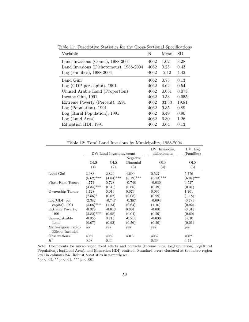
Table 11: Descriptive Statistics for the Cross-Sectional Specifications

Variable N Mean SD

Land Invasions (Count), 1988-2004 4062 1.02 3.28Land Invasions (Dichotomous), 1988-2004 4062 0.25 0.43Log (Families), 1988-2004 4062 -2.12 4.42

Land Gini 4062 0.75 0.13Log (GDP per capita), 1991 4062 4.62 0.54Unused Arable Land (Proportion) 4062 0.051 0.073Income Gini, 1991 4062 0.53 0.055Extreme Poverty (Percent), 1991 4062 33.53 19.81Log (Population), 1991 4062 9.35 0.89Log (Rural Population), 1991 4062 8.49 0.90Log (Land Area) 4062 6.30 1.26Education HDI, 1991 4062 0.64 0.13

Table 12: Total Land Invasions by Municipality, 1988-2004

DV: Invasions, DV: LogDV: Land Invasions, count dichotomous (Families)

NegativeOLS OLS Binomial OLS OLS(1) (2) (3) (4) (5)

Land Gini 2.983 2.829 4.609 0.527 5.776(6.62)*** (4.04)*** (6.19)*** (5.73)*** (6.07)***

Fixed-Rent Tenure 4.774 0.728 -0.748 -0.030 0.527(4.34)*** (0.41) (0.66) (0.19) (0.31)

Ownership Tenure 1.728 0.016 0.073 0.096 1.201(2.56)* (0.02) (0.08) (0.99) (1.18)

Log(GDP per -2.382 -0.747 -0.387 -0.094 -0.789capita), 1991 (5.06)*** (1.23) (0.64) (1.10) (0.92)

Extreme Poverty, -0.073 -0.013 0.001 -0.001 -0.0131991 (5.82)*** (0.98) (0.04) (0.59) (0.60)

Unused Arable -0.055 0.715 -0.514 -0.038 0.010Land (0.07) (0.92) (0.56) (0.29) (0.01)

Micro-region Fixed- no yes yes yes yesEffects Included

Observations 4062 4062 4013 4062 4062R2 0.08 0.34 0.39 0.41

Note: Coefficients for micro-region fixed effects and controls (Income Gini, log(Population), log(RuralPopulation), log(Land Area), and Education HDI) omitted. Standard errors clustered at the micro-regionlevel in columns 2-5. Robust t-statistics in parentheses.* p < .05, ** p < .01, *** p < .001

52