obtaining landmarks and semilandmarks -...

2

Obtaining Landmarks and

Semilandmarks

This chapter is about two steps of data collection - the first is obtaining the images to be digitized, the

second step is digitizing them. The MOST important decision that you will make about your data is

whether to use two- or three-dimensional coordinates. This decision will affect both the information

contained in your data and the mechanics of obtaining the data. There are many technologies for

collecting 3D data, and this advances so rapidly that anything we say is likely to be obsolete shortly. For

example, two years ago we might have said that microCT scanning was not well suited to very small

specimens such as rodent teeth, and that the most useful technology was the Reflex microscope. But the

development of high resolution computed tomography (sometimes called “nanoCT”) now makes it

possible to obtain 3D coordinates at the sub-micron level (Dhondt et al., 2010, van der Niet et al., 2010).

As a result, structures of very small specimens including very fragile ones such as shoots and flowers of

mouse-eared cress (Arabidopsis thaliana) can be recorded at a spatial resolution of 0.85 m in a scan

lasting approximately 1.5 hours. Of course, whether this method will be feasible for you depends on

many factors aside from the size and fragility of your specimens - it also depends on whether you (or your

specimens) can travel to a center where the technology is available (e.g. Belgium) and on your budget.

In general, the factors that determine the optimal technology for any research project include (but

are not limited to): (1) specimen size relative to the resolution and accuracy of the device; (2) specimen

fragility; (3) density of the tissues to image; (4) portability of the device and/or specimens; (5) ability to

obtain images of specimens versus just coordinates of landmarks; (6) ability to image landmarks on

2. Obtaining Landmarks and Semilandmarks

2

internal structures versus just the external surface; (7) cost of buying the device or per specimen cost of

having the imaging done; (8) labor; (9) training required to use properly the technology and/or software;

and (10) time available for data collection. Two-dimensional data are far less expensive to collect, takes

less time to obtain the images (and to digitize them) and the imaging device - the camera - is as portable

as you are. At present, most studies rely on 2D data, especially when analyzing large samples of small

organisms. Methods for collecting 2D data are now standardized whereas those for 3D data are not. We

therefore only briefly summarize methods now available for 3D data collection and then concentrate on

the most widely used method for acquiring 2D images (digital photography). The last part of this chapter

is on digitizing coordinates of landmarks in the most widely used digitizing program, tpsDig (Rohlf,

2010).

Methods for obtaining three-dimensional data

Three-dimensional data can be obtained in two basic forms (but the details of both forms can vary

considerably). The first is a set of coordinates digitized directly from the specimens - no images are

recorded - only coordinates are. Technologies that produce only coordinates include the 3D digitizers,

e.g. Microscribe (by Immersion Corporation), GoMeasure (http://gomeasure3d.com/wp/), and the

Polhemus digitizer (by Polhemus), and the Reflex Microscope (by Reflex Measurement;

http://www.reflexmeasurement.co.uk.). Below we call all of these the 3D digitizers because they are used

to obtain the x-, y-, z-coordinates. The second form is a digital 3D image from which coordinates (and

other information) can be extracted. Some imaging technologies penetrate the surface of the object and

allow you to visualize both surfaces and internal structures. These methods include x-ray computed

tomography (CT) and magnetic resonance imaging (MRI). Both produce “tomograms” - two dimensional

cross-sections or “slices”; the 3D image is reconstructed from a stack of those slices. Below we call these

the “penetrating scans”. Another imaging method, laser scanning, also reconstructs the 3D image from a

stack of slices, but does not penetrate the surface. This we call “surface scanning”. A third kind of 3D

imaging method works very differently from these others because it uses multiple 2D photographic

images to reconstruct the 3D image (photogrammetry and computer stereovision).

Three-dimensional digitizing

One type of technology for 3D digitizing uses a stylus, which is connected to the base by a

jointed arm (Microscribe; (http://www.emicroscribe.com/products/microscribe-mx.htm)) or a flexible

cord (Polhemus; http://www.polhemus.com/), which allows you to reach around, behind and under the

specimen. Digitizing is done by touching the tip of the stylus to the landmarks while the specimen is

fixed in its position. The movement of the jointed arm is measured by its degrees of freedom (df); 6 df

means that the arm can move forwards/backwards, up/down, left/right and rotate about three

http://www.emicroscribe.com/products/microscribe-mx.htm


3

perpendicular axes, with the movement along the axes and rotation about the axes being independent of

each other. 3D digitizers come in a variety of sizes and they vary considerably in accuracy; the most

accurate one (Microscribe MX) promises to be within ±0.002 inches (in) or 0.0508 mm of the true value.

The Polyhemus Patriot, promises less: an accuracy of only 0.05 in (1.3 mm). Even the most accurate 3D

digitizer, however, may be unsuitable for small, fragile specimens because the specimen has to be fixed in

its position - it must remain in precisely the same place while the stylus is moved around it. Fixing the

specimen can damage fragile material and, as Hallgrimsson and colleagues (Hallgrímsson et al., 2008)

point out, it can be a challenge to achieve the goal of a completely stationary specimen. For large

specimens, these devices can be attractive because they are portable, weighing as little as 12 lbs (5.4 kg)

in the case of the Microscribe MX, and they are also relatively inexpensive compared to other devices for

3D data collection. As priced today, the Microscribe MX, with 6 df, costs only $12,995.00

(http://www.emicroscribe.com/products/microscribe-mx.htm) and the Rhinoceros software adds only

$995.00 to the cost. They are also relatively simple to use and the coordinates can be obtained quickly.

The other 3D digitizing technology is the Reflex Microscope, which is a stereomicroscope.

When you look through the eye-pieces you will see a small dot, which you move into position over the

landmark using a joystick that moves the stage on which the specimen rests in the x and y directions. To

get the z coordinate, you move the microscope head up and down, using your stereoscopic vision to

position the spot on the landmark, which can be especially challenging when the surface is oblique to

your line of sight (if you have difficulty dissecting under a stereomicroscope, this technology may not be

for you). When the dot is properly positioned (or rather, when the specimen is properly positioned), the

coordinates are recorded by pressing a button on the joystick. The measurements have a very high degree

of accuracy, down to ±3 microns in the x and y direction, and ± 5 microns in the z direction. Thus, very

small specimens can be measured very accurately. The technology is not limited to very small objects,

however. Even specimens as large as 110 mm x 96 mm x180 mm can be measured by this device. The

size range that can be measured is described in the brochure provided by the manufacturer (Consultantnet

Ltd) as from vole teeth to primate skulls. However, their primate is a rather small one, a monkey skull.

This device is thus suitable for small to moderately large specimens. But even for small specimens, the

device has some limitations. First, it is not portable. Second, it is fairly expensive; no price list is

available on the manufacturer’s website, but one quoted by Dean (1996) in an overview of 3D

technology, was $35,000.00 and a more recent quote on the Stony Brook morphometrics website, current

as of 2001, is $41,000, although that includes a computer and software as well as the microscope and

case. Although it is not possible to record a 3D image of the specimen, it is possible to record 2D images

using the trinocular head that is available for video or photographic imaging.

http://www.emicroscribe.com/products/microscribe-mx.htm


4

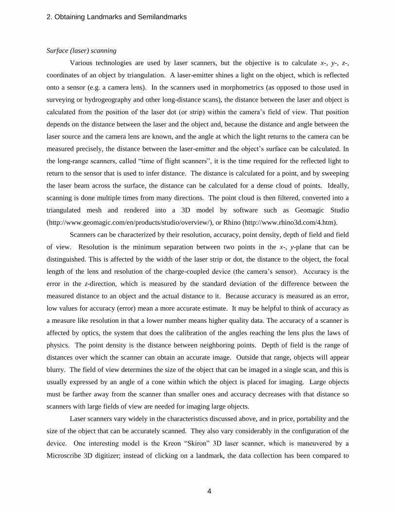
Surface (laser) scanning

Various technologies are used by laser scanners, but the objective is to calculate x-, y-, z-,

coordinates of an object by triangulation. A laser-emitter shines a light on the object, which is reflected

onto a sensor (e.g. a camera lens). In the scanners used in morphometrics (as opposed to those used in

surveying or hydrogeography and other long-distance scans), the distance between the laser and object is

calculated from the position of the laser dot (or strip) within the camera’s field of view. That position

depends on the distance between the laser and the object and, because the distance and angle between the

laser source and the camera lens are known, and the angle at which the light returns to the camera can be

measured precisely, the distance between the laser-emitter and the object’s surface can be calculated. In

the long-range scanners, called “time of flight scanners”, it is the time required for the reflected light to

return to the sensor that is used to infer distance. The distance is calculated for a point, and by sweeping

the laser beam across the surface, the distance can be calculated for a dense cloud of points. Ideally,

scanning is done multiple times from many directions. The point cloud is then filtered, converted into a

triangulated mesh and rendered into a 3D model by software such as Geomagic Studio

(http://www.geomagic.com/en/products/studio/overview/), or Rhino (http://www.rhino3d.com/4.htm).

Scanners can be characterized by their resolution, accuracy, point density, depth of field and field

of view. Resolution is the minimum separation between two points in the x-, y-plane that can be

distinguished. This is affected by the width of the laser strip or dot, the distance to the object, the focal

length of the lens and resolution of the charge-coupled device (the camera’s sensor). Accuracy is the

error in the z-direction, which is measured by the standard deviation of the difference between the

measured distance to an object and the actual distance to it. Because accuracy is measured as an error,

low values for accuracy (error) mean a more accurate estimate. It may be helpful to think of accuracy as

a measure like resolution in that a lower number means higher quality data. The accuracy of a scanner is

affected by optics, the system that does the calibration of the angles reaching the lens plus the laws of

physics. The point density is the distance between neighboring points. Depth of field is the range of

distances over which the scanner can obtain an accurate image. Outside that range, objects will appear

blurry. The field of view determines the size of the object that can be imaged in a single scan, and this is

usually expressed by an angle of a cone within which the object is placed for imaging. Large objects

must be farther away from the scanner than smaller ones and accuracy decreases with that distance so

scanners with large fields of view are needed for imaging large objects.

Laser scanners vary widely in the characteristics discussed above, and in price, portability and the

size of the object that can be accurately scanned. They also vary considerably in the configuration of the

device. One interesting model is the Kreon “Skiron” 3D laser scanner, which is maneuvered by a

Microscribe 3D digitizer; instead of clicking on a landmark, the data collection has been compared to

http://www.geomagic.com/en/products/studio/overview/

http://www.rhino3d.com/4.htm


5

“spray painting” (http://www.b3-d.com/Products.html); the scanner collecting 45,000 points per second,

at an accuracy of 16 m (.0006 in). This is presently listed at $18,659.00 to $21,995.00 (the price does

not include the Microscribe, which, for these systems ranges from approximately $6995.00 to

$29,990.00). Laser scanners can be both far cheaper and far more expensive than this. Among the

cheaper ones are some that are not limited by the size of an object because the object is placed in front of

it rather than inside it. Among these are the NextEngine 3D Laser scanner http://www.nextengine.com/),

costing only $4000.00 (with an accuracy of 125 m (0.005 in). The eScan, which can be found for as

little as $7795.00 ( http://gomeasure3d.com/wp/products/lbp/3d-laser-scanners-pp/escan-3d-laser-

scanners/) has a comparable accuracy of 150 m (0.006 in), which can be improved to 89 m (0.0035 in)

with an advanced lens.

Three-dimensional penetrating scans: X-ray computed tomography (CT scans) and magnetic resonance

imaging (MRI)

CT scanning and MRI are different modalities for obtaining 3D images of both surfaces and

interior points. CT scanning works by measuring the attenuation of the x-ray by the object. The

technique yields a set of slices (“tomographs’) which are reconstructed into a 3D image. At one time,

these were limited to slices along a single axis, but modern CT scanners use multiple detectors so the

objects can be reconstructed in all directions. MRI uses different pulses of radiofrequency energy to map

the relative abundance (and spin) of hydrogen nuclei in the presence of a strong magnetic field. The

radiofrequencies realign the magnetization so that the nuclei produce a rotating magnetic field that is

detected by the scanner. MRI is especially useful for distinguishing between soft tissues, but CT scans

can also be used to visualize soft tissues, and MRIs can also be used to visualize bones and teeth (and

both can be used on fossils). The stacks of slices produced by both methods are reconstructed into 3D

images by software such as Amira (http://www.amira.com).

CT scanners are more widely available, faster and less expensive than MRIs. MRIs are preferred

in medical applications when the specimens (patients) are living animals because MRIs do not expose

them to repeated doses of ionizing radiation. Both techniques have two major advantages over the other

methods discussed above. First, unlike the 3D digitizers, they produce images as well as coordinate data

and, unlike the surface (laser) scanner above, they provide information about internal as well as external

anatomy. Both have the disadvantage of being extremely expensive and of not being portable although

you may not have to take your specimens very far if your institution has a medical or dental school that

allows researchers to analyze (non-human) material. Usually, you would pay for the time of the

technicians who do the scanning plus for the software to reconstruct the images (and for a technician or

http://www.b3-d.com/Products.html

http://gomeasure3d.com/wp/products/lbp/3d-laser-scanners-pp/escan-3d-laser-scanners/

http://gomeasure3d.com/wp/products/lbp/3d-laser-scanners-pp/escan-3d-laser-scanners/

http://www.amira.com/


6

research assistant who is trained in using that software). Often, the time needed for scanning can be

reduced by packing many (small) specimens into a single tube.

Photogrammetry and stereovision

Photogrammetry and stereovision are techniques that rely on photographs to reconstruct three-

dimensional shapes. Like laser scanning, these techniques reconstruct only surfaces. Also like laser

scanning, triangulation is used to estimate the coordinates of landmarks (taken from multiple views).

Photogrammetry emcompasses a range of techniques that estimate the three-dimensional coordinates

from landmarks that are common to multiple photographs. The base of the triangle is the line between the

camera positions, and the sides of the triangle are rays that extend between each camera position and the

landmark on a specimen. This technique thus requires identifying landmarks that are visible in each view.

The coordinates are estimated as the points where the rays from camera positions to landmark intersect.

The estimates are affected by parameters intrinsic to the camera, especially its focal length and lens

correction as well as extrinsic parameters like the position and orientation of the camera. Both intrinsic

and extrinsic parameters must be calibrated before the coordinates of the landmarks can be estimated, and

the intrinsic parameters of the camera must be held constant between the calibration step and data

collection and throughout data collection (hence zoom lenses are discouraged). After photographing a

known object multiple times in multiple views, the intrinsic camera parameters can be determined. Once

both intrinsic and extrinsic camera parameters are estimated, a 3D surface consisting of polygons

connecting the landmarks is reconstructed.

A surface reconstructed from just a few polygons will not accurately reconstruct a complex,

curving surface just as a complex 2D curve will not be well reconstructed by a small number of straight

lines. A landmark-poor morphology is not a good candidate for this method. It is, however, an

inexpensive method for obtaining 3D data and the system is highly portable. It can even be used under

field conditions - one of the most interesting applications is a field study of tortoise carapace morphology

(Chiari et al., 2008). The live animals were photographed under natural conditions; as the authors point

out, these animals do not move quickly. However, their carapaces offer few landmarks; the landmarks

were located at intersections between scutes and only two landmarks were at intersections with peripheral

scutes. As a result, the deviations between geodesic distances measured by flexible tape and those

reconstructed by photogrammetry were exceptionally large, on the order of 15-20 mm.

Stereovision differs from photogrammetry primarily in the density of points used in

reconstructing the 3D coordinates. Like photogrammetry, it uses partially overlapping views of an object,

but these views are stereoimage pairs captured by two cameras at a known distance from each other (they

may even be bolted to each other). Multiple partially overlapping stereoimage pairs are taken, and these


7

are used to reconstruct the portion of the specimen that is visible in both images. During the processing

stage, the reconstructed partial images are aligned with each other (by specifying the locations of three

corresponding points in the pairs). The method is therefore not limited by the number of landmarks or

their spacing because landmarks are necessary only for aligning the partial models and only three (per

partial model) are used for that purpose. This method may be less useful under field conditions, but

Chiari and colleagues found that the method performs better than photogrammetry.

Both approaches are relatively inexpensive. The only costs are the camera(s) and modeling

software. For stereovision modeling, two cameras are needed as well as the software, but the pair of

cameras (synchronized stereo head, with a variable baseline) made by Videre Designs are listed at $2000

(http://users.rcn.com/mclaughl.dnai/) and bundled with SRI International’s Small Vision System.

Photogrammetry requires only one camera; the program widely used for reconstructing 3D images,

Photomodeler, is presently listed at $1145.00 (http://www.photomodeler.com/index.htm).

Obtaining two-dimensional data

The important (and obvious) difference between 2- and 3D data collection is that 2D photographs of 3D

objects project that object onto a plane. If objects are not consistently oriented, the projected images will

seem to differ in shape even when they differ solely in orientation. Thus, the first step in 2D data

collection is to figure out how you will ensure a consistent orientation for your specimens. That will

obviously depend heavily on the morphology of your specimens. If they are truly flat, or nearly so (such

as the mandibles of mice split at the symphysis), you can just place them on the copy stand alongside a

ruler (or even use a flat-bed scanner). However, if they are more nearly round, such as the crania of mice,

you will need both a method for positioning them and for maintaining them in place. If you are traveling

to various museums to collect data, you need a portable device that can ensure consistent position. Before

you begin to collect data, you should take multiple photographs of the same specimen, placing it into

position for each photograph, so that you can estimate the error due to positioning. If you photograph the

same image 10 times, and digitize each image 10 times, you can assess the error due to positioning and

digitizing (by the variation explained by each).

Included below are the rudiments of taking a picture (what makes the image and how can you

manipulate the camera and the lighting to get a better image), and a few things you can do to make the

captured image even better in photo editing software. Although the range of hardware and software has

become fairly standardized, most of the following discussion is quite general. You will need to

familiarize yourself with the characteristics of your particular system (but then, you will need to do that

anyway to get the best possible results). Our goal is to provide you with an orientation to the subject that

gets you through the first stages of that familiarization with a minimum of unnecessary pain.

http://users.rcn.com/mclaughl.dnai/

http://www.photomodeler.com/index.htm


8

Inside the camera

The aperture. Arguably, the most important part of a camera is the aperture - the small hole that

lets light into the box to form the image. The aperture is critical because light reflecting off the object is

leaving it in many different directions. The aperture functions as a filter that selects light rays based on

their direction of travel. The only rays admitted into the camera are the ones traveling on the path that

takes them through the aperture. In theory, if the aperture is small enough (and nothing else intervenes),

it insures that the geometric arrangement of the rays’ starting locations is exactly reproduced by the

geometric arrangement of the rays’ arrival locations (Figure W2.1). This is why a child’s pin-hole

shoebox camera works. It is also why the image is inverted.

Because the image is formed from a cone of light leaving a three-dimensional object and arriving

on a 2D surface, there are certain artifacts or distortions introduced in the image (Figure W2.2). As

discussed below, a good lens system can reduce these effects, but it cannot eliminate them completely.

One distortion in photographic images of 3D objects is that an object closer to the camera will appear to

be magnified relative to an object that is farther from the camera (Figure W2.2A). This occurs because

the light rays traveling toward the lens from opposite corners of the object form a larger angle when the

object is closer to the aperture, which means they will form a larger image inside the camera. For this

same reason, the closer feature will hide more distant features. Another distortion is that smaller objects

in the field may appear to be behind taller objects when the smaller objects are actually next to the taller

object (Figure W2.2B). The reality is that the smaller object is farther from the aperture, but not in the

expected direction. In a related phenomenon, surfaces of an object that face toward the center of the field

of view will be visible in the image, and surfaces that face away from the center will not be visible

Figure W2.1. Image formation in an idealized pin-hole camera. Light rays travel in a straight line from a

point on the object (the squirrel jaw) through the aperture to a point on the back wall of the box. The

geometric arrangement of the starting locations of light rays and their reproduction by the rays’ arrival

locations.


9

Figure W2.2. Distortions resulting from light leaving a three-dimensional surface and arriving on a two-

dimensional plane. A: The two rectangles have the same width but the upper (“taller”) rectangle produces

a larger image (appears to be magnified) because its end is closer to the camera. B: An object that is

farther from the center appears to be behind an object that is closer to the center of the image, especially if

the more central object is “taller”. C: The sides of an object that face the center of the field are visible

and the surfaces that face away from the center are hidden. In the special case of a spherical object, less

than half of the surface will be visible; if the object is not centered in the field, the apparent horizon will

be tilted away from the expected reference plane (the equator) toward the aperture.

(Figure W2.2C). This is the reason buildings appear to lean away from the camera in aerial photographs.

In the case of a sphere, this means that the visible edge (horizon) will not be the equator, but will be

closer to the camera than the equator. If the sphere is not centered in the image, the horizon will also be

tilted toward the center of the image (this effect can be a serious obstacle to digitizing landmarks on the

sagittal plane of a skull). These phenomena are more pronounced near the edges of the image, so one

way to reduce their influence on your results is consistently to center your specimens in the field of view.

Near the end of the next section we discuss other steps you can take to minimize these distortions and the

effects they would have on your morphometric data.

What the lens does. The lens does two things: it magnifies the image, and it makes it possible to

use a larger aperture than a pin-hole. Both are important advantages, but they come with a cost. The size

of the image in a pin-hole camera is a function of the ratio of two distances: (1) the distance from the


10

object to the aperture; and (2) the distance from the aperture to the back of the box. If the object is far

from the pin-hole, light rays converging on the aperture from different ends of the object will form a

small angle. The light rays will leave the pin-hole in the same small angle, so the image will be smaller

than the object unless the box is very large. One way to enlarge the image is enlarge the box, another is to

shorten the distance between the camera and the object, so that light rays converging on the aperture from

different ends of the object will form a very large angle covering of the back surface (Figure W2.3A). A

lens magnifies the image by changing the paths of the light arriving at the lens so that the angle between

them when they depart the lens is greater than the angle between them when they arrived. Consequently,

the image is larger than it would be without a lens, making the object appear to be closer to the lens than

it is (Figure W2.3B).

The amount of magnification produced by a lens depends on several factors. Light striking the

surface of the lens at 90° does not change direction but, as the angle of incidence becomes more acute, the

change in direction increases. Exactly how much the path of the light is bent depends on the properties of

the material of which the lens is made and on the wavelength of the light. The light changes direction

Figure W2.3. Two methods of image magnification. A: Moving the camera and object closer together. B:

Using a lens to change the paths that the light travels from the object to the image, thereby changing the

apparent distance of the object from the aperture.

again when it exits the lens. In addition to the advantage of having a larger image, which enhances

resolution, there is the additional advantage that the distortions that occur in images of 3D objects are

reduced. Because the object is farther away than it would be for a pin-hole image of the same


11

magnification, the same small aperture is now selecting a narrower cone of rays leaving the object. This

is particularly true for features near the center of the image. Features near the edges of the image are

subject to other distortions (see below).

The image in a pin-hole camera is faint because the pin-hole must be small to be an effective

filter of the light rays’ directions of travel. A larger aperture would admit more of the light leaving the

object, but it would produce a fuzzier image because a larger cone of light leaving each point on theobject

would reach the back of the box (Figure W2.4A). Consequently, features in the image would have wide

diffuse edges, and the edges of adjacent features would overlap, making it impossible to discriminate

between those features. The lens corrects this problem by bending the light so that the cone converges

again at some point on the other side of the lens (Figure W2.4B). This allows you to increase the size of

the aperture, allowing more light from the object to reach the back of the box. The image that results is

generally brighter and has more contrast between light and dark areas.

Figure W2.4. The role of the lens in enhancing image resolution. A: A large aperture admits many rays

leaving the object in divergent directions, which produces a fuzzy image because each point on the object

produces a relatively large circle of light at the back of the box. B: The lens bends the light so the

diverging rays from a point on the object converge on a point at the back of the box.

The principal cost of using a lens is that it imposes a particular relationship on the distances from

the lens to the object and the image. This relationship is expressed by the following equation:

1/f = 1/do + 1/di (2.1)


12

Where do and di are the distances to the object and image, respectively. The value of f is

determined by the shape and material properties of the lenses, and is called the focal length. For the cone

of light from a particular point on the object to converge again at the back of the camera, that point on the

object must be a specific distance from the lens. At this distance, that point is “in focus.” If a part of the

object is not at this optimal distance, light leaving that part does not converge at the right distance behind

the lens, and that part of the image is blurred. The thickness of the zone in which this effect is negligible

is the depth of field. Greater depth of field means that a thicker section of the specimen will be perceived

as in focus. Depth of field decreases with magnification. At higher magnification, the light is bent more

as it passes through the lens, so the difference in focal points is magnified as much as the areas of the

features. Consequently, a thinner section of the specimen is in focus. To complicate matters further, in

simple (single-lens) optical systems, the slice that is in focus is curved, not flat. Similarly, the surface on

which the image is in focus is also curved. The complex lens systems of higher quality optical equipment

flatten these surfaces considerably, but you may still find that only the center of a flat object (or a ring

around the center) is in focus. The best solution for this problem is to use a lower magnification,

increasing the depth of field. There are things you can do to edit the “captured” image but, as we discuss

in a later section, these are limited by the initial quality of the image.

Near the edge of the image, additional distortions produced by the lens may become apparent.

These distortions arise because the amount that the path of light is bent is not just a function of the

properties of the lens. The deflection is also a function of the angle of incidence and the wavelength of

the light. Two rays arriving at the center of the lens from locations near the center of the field of view are

bent by relatively small amounts because they strike the surface at nearly 90°. Two rays arriving at the

lens from locations near the edge of the field of view are not only bent by larger amounts, the difference

in how much they are bent is also greater. Consequently, a straight line passing through the field will be

curved in the image unless it passes through the center of the field. Closer to the edge of the field,

differences in how much different wavelengths of light are bent by the lens may also become apparent as

rainbows fringing the edges of features in the image. This is effect is most evident under high

magnification or very bright light.

Checking your system

The complex lens systems of higher quality optical equipment greatly reduce all of the distortions

discussed above, but none of these distortions can be eliminated completely. Fortunately, there are a few

simple things you can do to insure that the effects on your data are negligible. The first is to put a piece

of graph paper in the field and note where the rainbow effect, if any, becomes apparent. Next, digitize

several points at regular intervals along a line through the center and compute the distances between the


13

points. As you approach the edge of the image, the interval will gradually change. Take note of where

this effect begins to be appreciable; you will want to keep the image of your specimen inside of this

region. In other words, if the object is large, place the camera at a greater distance so that the image does

not extend into the distorted region of the field. Next, get a box or other object with a flat bottom and

vertical sides and mark one side of the box at a height corresponding to the thickness of your specimens.

Put the box in the field of view, with the marked side at the center of the field. Slowly slide the box

toward one edge of the field until you can see the inner surface of the side between the mark and the

bottom. Again, you will want to keep your specimens inside this region. Outside of this region, features

at the height of the mark will appear to be displaced away from the center of the image. Finally, check

your depth of field by putting a sloped object marked with the thickness of your specimen (or one of your

larger specimens) in the field. If all the critical features are not in focus at the same time, you should use

a lower magnification to avoid guessing where in the fuzz is the feature you want to digitize.

What happens in the back of a camera

Now that you have a minimally distorted image at the back of your camera, you need to “capture”

the image with a light sensitive device (the detector array). These contain a large number of light

detectors used to record the image (pixels); a bundle of three light-sensitive devices recording intensities

in three narrow color ranges. The higher the number of detectors, the higher the resolution of the

recorded image. The image captured by your camera is not the image you digitize. What you see on the

screen is a second image reproduced from the information collected by the detectors. If the camera image

is mapped to the screen 1-to-1, pixel for pixel, the two images will have the same resolution. You can

enlarge or reduce the image but you cannot increase its resolution. When the screen image size is

reduced, information from multiple camera pixels is averaged for display by a single screen pixel. This

may produce an image that looks sharper, but that loses the small-scale, almost imperceptible details that

created the original “fuzz”. The reduced picture may be easier to interpret but at the risk of merging

features you want to digitize. When the screen image is enlarged, information from a single camera pixel

is displayed by multiple screen pixels. This produces the blocky, stair-step effect. The result seems less

resolved because the edges are not smooth, but features that were separate before still are separate. The

drawback is that excessive enlargement may make the image difficult to interpret and increase the mental

strain of digitizing.

Saving image files

Once you have an image “captured”, you must decide how you want to save it. One option, often

the default, is to use your camera-specific format for raw (unprocessed) photographs, e.g. *.NEF for

Nikon, *.MRW for Minolta). In general, these contain more information than any processed photograph;


14

they are 16-bit rather than 8-bit, and therefore have more detail. Most raw files can be read by photo-

editing programs, although which ones can be read depends on the photo-editing programs (and the

freeware programs may be more limited than the ones that you pay for - so check your photo-editing

program if you do not want to invest in another). As of this writing, the raw formats cannot be read by

the tpsDig. If you save your images in the camera-specific raw format, you will later need to convert it

into a standard format (e.g. *.JPG, *.TIF) but you can take advantage of the greater information contained

in the raw photographs when enhancing the image. However, if you cannot easily download the images

when the camera is full, you might prefer to save smaller files, e.g. *.JPGs, while taking the photographs.

You will lose information when the file is compressed into a JPG, and you will actually lose information

each time you save a JPG because it is compressed each time it is saved. You might instead want to save

TIF files (but these too are very large).

Most standard image file formats are raster formats (also called bitmap formats). In these

formats, the image is represented as a set of values assigned to a grid. This format reflects the structure of

your screen and the detector array in your camera. BMP, TIF and JPG are all raster formats. The

principal alternative is the vector format in which the image is represented by a series of mathematical

formulae that specify a set of geometric shapes. This format has some advantages over the raster format,

but it does not work well with photographic images of biological specimens because the complexity of

these specimens requires a large number of geometric shapes to be mapped onto the specimen. Meta

formats, such as that used in Windows metafiles (*.WMF), allow data in multiple formats in the same

file, permitting the user to build up complex compositions (e.g. a picture, plus a graph, plus text).

The quality of an image reproduced from a raster file depends on the number of bits used to save

the information at each cell (pixel) in the grid. The number of bits determines the number of colors or

gray tones in the image. A 16-bit image can contain up to 64K colors, an 8-bit image can contain only

256 colors. Each pixel displays only a single color, so the advantage of the 16-bit image is that it can

have much smaller changes in color from one pixel to the next. Thus, the 16-bit image can more

accurately reflect graded changes in color across the object. In practice, the 8-bit image may not be

noticeably poorer unless the image size is changed, and the 8-bit image file would have the advantage of

requiring much less disk space in your camera (and on your hard disk). The most economical format is

JPG (Joint Photographic Experts Group, JPG). This is a compressed format analogous to the *.ZIP

format. An image that requires 900K of disk space as a 16-bit BMP or TIF file might require less than

100K as a minimally compressed JPG. More important, the 100K JPG will look just as good on the

screen because there is very little information lost in the compression. In contrast, a 4-bit BMP file

requiring about the same disk space will have lost much more information and look considerably worse.


15

If you have room in your camera’s memory, keep the files in raw format and save them in that format to

your hard disk. Then you can convert the files to JPGs without losing the original raw file.

If you are really pressed for disk space but need to preserve as much color information as you

can, explore the options in your software. Normal color reduction replaces each pixel with the nearest

color in the reduced color set (e.g. emerald, jade and lime will all be replaced with green). This creates

large blocks of uniform color that obliterate many details. Various optimizations and diffusion algorithms

produce “speckled” images that blend into more natural colors when viewed at a distance, or when

reduced. These also do a better job of preserving edges.

Improving the image

Before you take the photograph

What you see in the image depends on how much light you shine on the object and how much of

the light reflected from the object you allow to reach the detector. There are several options for

manipulating light; the trick is to find the right balance so that you can see the features you want to

digitize. It is important to understand that the best image for digitizing may not be the most esthetically

pleasing image.

When you shine a light from a single source on a three-dimensional object some parts are likely

to be in shadow. Shadows can be advantageous in that they allow you to see the relief; but you want to

avoid a shadow so dark that you cannot see anything in the shadow. Backlighting allows you to see

features in the shadow without obliterating the shadows. This is achieved by using a weaker light, or

some kind of reflector (e.g. a piece of white paper) to illuminate the “back” of the object.

The size of the aperture and the amount of time it is open determine the amount of light that

strikes the detector. A larger aperture admits more light but, as discussed above, the image is less sharply

resolved. However, minimizing the aperture does not necessarily produce the most useful picture. A

small aperture allows very little light to reach the detector from any area and the resulting image is

generally dark. You can compensate for this by decreasing the shutter speed (or its digital analog). This

allows light through the aperture to register on the detector for a longer period of time. As the shutter

stays open longer, the brighter parts of the specimens become brighter in the image and the dark parts of

the image stay dark. In other words, the contrast is increased. Unfortunately, minimizing shutter speed

does not necessarily produce the best picture either. The longer the time that light is collected, the longer

the fuzzy fringes register on the detector. If you leave the aperture open too long, eventually thin dark

features will be obliterated completely and small bright areas will appear larger than they really are. You

can also compensate for small aperture size by using brighter lights to illuminate the object. This has


16

much the same effect as increasing the time the aperture is open. More light registers because there is

more light from the specimen per unit time.

In summary, getting a decent picture may require a delicate and sometimes annoying balancing

act. We strongly recommend that you try many different settings to see what works best and keep a log

of the conditions in which each picture was taken. In your log, you should also take note of the

brightness and shininess of the specimen. A dull gray specimen may require a different set-up than a

shiny white specimen. You should also take note of what other room lights are on. If the room where

you are working has windows, the time of day can be an important factor, as well. Have patience.

Although there is a lot you can do to edit an image, you can only highlight information that is already

there. You can’t recover information that was lost by the original.

After you have taken the photograph (photo-editing).

A quick tour through almost any photo-editing software will reveal a bewildering array of

functions you could use to modify your image. Here, we discuss a few tools that are widely available and

will likely to be useful to a large number of biologists. Many of these manipulations reduce the accuracy

of the image as a reproduction of the original image. Again, it is important to realize that an esthetically

pleasing or artistically interesting image may not be the best one to digitize for a morphometric analysis.

Probably the two most generally useful tools are the ones that adjust brightness and contrast.

These functions can be most easily understood if your image editor displays a histogram of pixel

luminance (the intensity of light emitted). Increasing brightness makes the whole image lighter, adding

the same increment of luminance to every cell, up to the maximum value. Detail is lost at the bright end

because pixels near that end converge on the maximum value. Details at the dark end may emerge as they

are brought into a range where the differences between adjacent cells become perceptible. Except for the

pixels near the bright end, the actual difference in brightness between adjacent cells does not change (the

peaks in the histogram move toward the bright end, but they do not change shape). Decreasing brightness

has the opposite effect. Increasing contrast makes the dark areas darker and the bright areas brighter,

shifting the peaks away from the middle, towards the ends. Decreasing contrast makes everything a

homogeneous gray, shifting the peaks toward the middle. The peaks also change shape as they move,

becoming narrower and taller with decreasing contrast, and wider and flatter with increasing contrast.

Again, differences between adjacent cells are lost as their values converge on the ends or the middle.

Adjustments of either brightness or contrast can be used to make features near the middle of the

brightness range easier to distinguish. The difference is whether the features that are made harder to

distinguish are at one end (brightness) or both ends (contrast) of the range.


17

As noted above, raster formatted images have jagged edges. When the image is scaled up, it is

also apparent that sharp edges in the original are represented as transition zones with large steps in

brightness and/or color. This creates the problem of deciding exactly where in the zone is the edge you

want to digitize. Adjusting brightness is unlikely to solve this problem because the number of steps and

the difference between them stays the same. Increasing contrast can help more, because it makes the

steps bigger. This comes at the expense of making the jaggedness more apparent. Even so, narrowing the

zone of transition may be worth the increased jaggedness. Some alternatives to increasing contrast may

include sharpening and edge enhancement. These tools use more complex operations that both shift and

change the shapes of the luminance peaks, but they also can produce images with thinner edges. In

general terms, the effect is similar to increasing contrast, but the computations are performed on a more

local scale. Which tool works best to highlight the features you want to digitize will depend on the

composition of your picture. Consequently, what works for one image may not work for another.

Additional photo-editing steps

As well as enhancing the images, you may want to edit the photographs further to make digitizing

easier. One step that does not alter the image - renaming the files so that each one has a unique (and, if

desired, recognizable) name. The others do alter the images. One step that makes the files easier to load

and also to navigate is cropping; this eliminates the excess background, which both reduces the size of the

file and makes it unnecessary to hunt for the specimen as you scroll through the file (which you will do

when digitizing). Another is flipping or otherwise reorienting the photographs to standardize the

orientation that you see when you digitize the image, which also standardizes the physical process of

digitizing. Finally, you can resize the images if the files are very large by fixing the number of pixels

(either by width or height).

Renaming the photographs with a recognizable and unique identifier, such as the specimen name

or number, serves two purposes. First, it solves the problem of having several specimens with the same

filename (e.g. DSC_0001.JPG). Each time you download the photographs from the camera, it will restart

at DSC_001.JPG and if you save the new DSC_001.JPG to the same folder, it will overwrite the one

already there. You can avoid that problem by keeping the images in different files, but that will

eventually create a problem when you digitize the images - either you will need to digitize several folders

of files separately or you will have to include the full path name of the file in the file name. Second,

naming the files with relevant information allows you to recognize the images as you digitize them and to

sort data files later. The filename is shown along with the photograph when you are digitizing them in the

most commonly used digitizing program tpsDig (see below), and it is included in the output of that

program. Additionally, you can get a list of all the filenames of the photographs using another program in


18

the tps series, tpsUtil. If the name of the image file contains useful information, you will know what you

are digitizing while you are digitizing, and you will able be able to sort your data file as you add (or

remove) specimens from them. If you do not want to know what you are digitizing while you are

digitizing, you can give each specimen a code instead of a recognizable label.

Cropping is useful if your specimens take up relatively little space in the picture or, more

importantly, if they take up different amounts of space. Cropping them so that all specimens take up

approximately the same space in the picture, and resizing the images to a standard image size, makes it

easier to go from one picture to the next without adjusting the magnification in tpsDig. It is particularly

useful to crop and resize when image files that are larger than about 4M open slowly (if at all) in tpsDig.

However, if you did not include a ruler in the image, but did photograph them all at a standard distance

(and magnification), do not adjust the size of the photograph. Under those conditions, the only

information that you will have about size is the actual size of the photographed specimen. You should

crop the images before enhancing brightness and contrast so that you are enhancing the image of the

specimen not the background. Once cropped, it is useful to resize the images; saving the processed files

as TIFF files will ensure that they will not lose information. But TIFF files are very large. After

cropping the images, you can save the image at 1000 pixels wide.

Reflecting (or perhaps also rotating) the specimens is useful if they were photographed in

different orientations. You do not need to perform either step. You can reflect specimens (i.e. flip them

either horizontally or vertically) while digitizing. In tpsDig, there is a function in the Image tools menu

(on the Options menu) for flipping the images, which are then saved by going to the File menu and

selecting “Save Image”). A particularly useful feature of this program is that you can flip the images

after digitizing them because the data will flip with the specimen. You can flip them later after you have

finished digitizing the specimens by opening the file in a spreadsheet and multiplying the x or y

coordinates of every landmark by -1 according to the orientation that you want to reverse. However, if

half the specimens face left and half right or half face up and the other half down, digitizing is less

straightforward because you will not develop a reliable search image and the physical process of

digitizing (especially that of tracing curves) can introduce subtle variation in the handedness of the

images that might look like asymmetry of the specimen. This is why you might also want to standardize

the orientation of your specimens if you did not do that while photographing them. If you are digitizing

landmarks that are recognizable as inflection points on curves, having the curves in different orientations

may make it difficult to recognize those inflection points.

After editing the images, rename them and save them in the desired format; TIF files have the

advantage that they lose no information when you reopen and close them, but they have the disadvantage

of being very large. If you plan to save them as TIF files, resize the image (e.g. to 1000 pixels wide). If


19

your program offers you the option of using LZW compression, do not select it; the files will not open in

tpsDig.

There are many photo-editing programs, just make sure yours does not lose information, or

worse, distort the image, which can happen if you rotate them. Microsoft viewer is not adequate for this

purpose, but you can find freeware photo-editors that are (e.g. GIMP, http://www.gimp.org/) Paint.net

(http://www.getpaint.net/) or Serif PhotoPlus Starter Edition (http://www.serif.com/FreeDownloads/). An

important limitation of free programs is that they usually do not allow you to write scripts for repetitive

tasks (e.g. adjusting brightness and contrast, rotating the images, sizing them to 1000 pixels, and saving as

TIF files). In some cases, features (including scripting) are disabled to encourage you to pay for the full

version. The full version of Serif PhotoPlus is presently $89.99, which is modest compared to PhotoShop

(presently listed at $699.00 http://www.adobe.com/products/photoshop/buying-guide.html). If you find

yourself spending a lot of time editing your photos, you should look at several of the freeware programs

because some are more intuitive than others. Look for a program that allows you quickly to crop, adjust

levels and contrast, flip the image both vertically and horizontally, resize the image and save it to your

desired file type. If you save your images in raw format, you also want to make sure that the program can

read it.

Digitizing in tpsDig

This discussion of digitizing focuses on how to use one particular program, tpsDig. We recommend it

not only because it is an excellent program but also because virtually all programs for shape analysis can

read data in the format output by this program. Therefore, you will not need to reformat the data before

you can analyze it. Also, tpsDig, especially the most recent version of it, includes useful functions that

other digitizing programs do not have. As of this writing, there are two versions of this program available

on the Stony Brook morphometrics website, tpsDig1.4 and tpsDig2.16. In general, tpsDig2.16 is the

more useful one, but it is also worth having TpsDig1.4 because you may find that one essential task is

easier to perform in that version (set scale), another is more convenient to use in that version (the template

function), one editing step is easier to do in that program (insert landmark) and one other is often possible

only in that version (delete landmark) after the semilandmarks have been resampled.

We first describe how to prepare the data file before digitizing, using another program in the tps

series, tpsUtil, an exceedingly useful utility program. Once that empty data file is made, it is then opened

in tpsDig and the coordinates are written to that file. Finally, we describe how to digitize and edit the

semilandmark curves and how to turn them into data (they are simply background curves when you first

digitize them). Semilandmarks do not have to be digitized last (i.e. after digitizing all the landmarks), and

they do not have to be digitized as curves, but there are advantages in doing both. One advantage of

http://www.gimp.org/

http://www.getpaint.net/

http://www.serif.com/FreeDownloads/

http://www.adobe.com/products/photoshop/buying-guide.html


20

digitizing them last is that you may change your mind about where the landmarks should be placed, which

would mean editing the semilandmark curves that lie between any repositioned landmarks. The other is

that you will need to use tpsDig2.16 for digitizing semilandmarks, but you may wish to use tpsDig1.14

when you digitize the landmarks because this program can be easier to use. If you digitize all the

landmarks first you will not need to switch from one program to the next as you digitize each specimen.

One important feature of these programs is that the files are upwardly and downwardly compatible so you

actually can switch between them.

Getting ready to digitize your first image:Preparing an empty data file in tpsUtil

Before you begin digitizing, it is a good idea to create a file that will contain the data. This step is

not essential because you can always open an image file, digitize it and save its coordinates to a file, then

do the same for the next and all remaining images, either saving each one to a separate file or appending

each one to the same file. But putting each specimen in a different data file means that you will have to

keep track of all the specimens that you have already digitized so that you neither forget to digitize some

nor inadvertently digitize the same one multiple times. Appending each file as you go is quite risky

because, when you go to save the image, the pop-up menu will give you the options to append or

overwrite the file, and mistakenly clicking on overwrite will replace all the data that you have already

digitized for all specimens with the data for the one specimen that you just digitized. This may seem like

a difficult mistake to make, but making it only once means that you’ve lost all the work done to that

point.

By creating an empty data file, to be filled with the data for all the specimens, you can ensure that

every specimen is included in the file (and only once) and you will also be able to navigate the file and

look at all the specimens in it. That can be especially useful when you need to check the consistency of

your digitizing - sometimes, a landmark can migrate over the course of digitizing and landmarks are

sometimes digitized out of order. You can check for digitizing error by running a principal components

analysis of the data (do not worry if, at present, you do not understand what a principal components

analysis is). If you run the analysis and see a single specimen very far from the others, you can go back

to the file and check it. At first sight, it may look like all the others because no landmarks are obviously

out of place but, if you look at the numbers next to the landmarks, you’re likely to find that they are in a

different order in that outlier.

The empty data file will contain the control lines for the tpsDig program; it will look like this:

LM=0

IMAGE=Aml_1508LC.jpg

ID=0

LM=0

IMAGE=Aml_1508LC.tif


21

ID=1

LM=0

IMAGE=Aml_1512LA.jpg

ID=2

(etc.)

The first line (LM=0) gives the number of landmarks, which is zero because none have been

digitized yet. The second is image filename, and the third is the ID number for the specimen, which

begins with zero (because the programming language C counts from zero). After digitizing a specimen,

the number of landmarks is replaced by the number that you digitized and its coordinates follow that

number (arranged in two columns, the x and y coordinates for each landmark). If using the scale function,

the scale factor is the last line in the file.

LM=16

552.00000 729.00000

464.00000 914.00000

691.00000 797.00000

925.00000 808.00000

955.00000 943.00000

1064.00000 953.00000

1132.00000 962.00000

1561.00000 1032.00000

1705.00000 1329.00000

1811.00000 1182.00000

1941.00000 1137.00000

1889.00000 771.00000

1950.00000 1106.00000

822.00000 919.00000

1285.00000 644.00000

1215.00000 974.00000

IMAGE=Aml_1508LC.jpg

ID=0

SCALE=0.001515

LM=0

IMAGE=Aml_1508LC.tif

ID=1

LM=0

IMAGE=Aml_1512LA.jpg

ID=2

You can prepare the empty file using tpsUtil (which has many other useful functions that you

should look at while you have it open). Start tpsUtil and, from the Operation menu, select the function

build tps file from images; which is presently the first option on the list. Then select Input file or


22

directory; go to the folder where you have your image files and select one of them (it does not matter

which one). Then name your output file and select the format for that file (i.e. tps or NTS). We

recommend tps format because virtually every morphometrics program can read it. Then click the SetUp

button, which will give you a list of all the image files in your folder and various options (such as Include

All or Exclude All). The default is to include all, but you can deselect any that you do not want to

include. If you want to include just a few, you can click Exclude All then pick the ones that you want to

include. You can choose the order of the images in the file using the Up and Dn (down) arrows or sort

them (using the Sort function). If you select Include path?, the full path will be included in the

filename, which is convenient when you want to keep the data file in a different folder from the images.

However, doing that can complicate moving image files to a different folder (because that will change its

path name) and it can also make it difficult to read the filenames in tpsDig because they will be too long

to display fully.

After you have selected all the images that you want to include in that file, select Create. The

file that you create is the one that you will open in tpsDig. Before leaving tpsUtil, you might want to

produce a file that lists the image files included in the data file (you can do this now or later or both). You

will want a record of the specimens in that file, especially if you begin to accumulate many data files and

cannot recall which specimens are in which. You will likely want to do this again at the end of digitizing

if you deleted any specimens from your file as you digitized. To produce this file, go to the last option in

the Operation window, List images in the tps file go to the Input window and load the file that you just

created, go to the Output window and name the file (it will be a comma delimited *.csv file), and name it

with a *.csv extension, then click Create.

Digitizing in tpsDig

The mechanics of digitizing depend partly on which version of tpsDig you use, but many of the functions

work the same in both versions. We will not cover all the functions that these programs have because we

are not familiar with them all. If you are interested in making measurements of linear distances, angles or

areas, or measuring the lengths of outlines, look at the various functions that you can find in the Modes

and Options menus (and it always does help to read the Help file). The first step is to open the file that

you made in tpsUtil, or if you did not make a file, to open an image file. In tpsDig2.16, go the File

menu, select Input source, then File. If you made an empty data file, open it; if you did not make a data

file, find the image format for your photos (e.g. JPG or TIFF) on the Files of Type list and select that, and

choose the first one to digitize and click Open. An image should appear in the main window. You can

zoom in or out using the buttons + and – on the top right of the toolbar, where you will also see a number

that shows the magnification of the image.


23

Before you start digitizing, you may want to change the cursor. This is what you will place on

the landmarks so you want to select a cursor that makes it easiest for you to locate the cross-hairs of the

cursor (or the arrowhead) most precisely. Go to the Options menu and select Image tools. In the window

that opens (and may immediately minimize), select the Cursors tab and choose the digitizing cursor that

you prefer. You can try out the cursor by moving it over the image but do not click on a point unless you

are on the first point that you plan to digitize; if you click, the coordinates of that point will be recorded in

the file and the image tools window will close. When you find the cursor that you like best, you can

select the color that you want the landmarks to be using the Colors tab. You can also select the size of the

circle that will be used to indicate a landmark’s position, and whether the circle will be closed or open, as

well as the color and size of the number used to label the landmark. You can change these options at any

time. Close this window and you are now ready to digitize.

To begin digitizing, find the image of the cursor (the circle with the cross-hairs) on the toolbar, or

Go to the Modes menu, and select Digitize landmarks, and go to the Options menu, and select Label

landmarks (this will put numbers next to the digitized points). Position the cursor over the landmark and

click the left mouse button. A circle and number should appear. To digitize the next landmark just

position the cursor at the appropriate point and left-click; keep going until you have finished digitizing all

the landmarks that you plan to do before going on to the next specimen.

At this point, you should make a screen shot of your digitized landmarks, with visible numbers so

that you will have a reminder of their locations and sequence. You can print the image and save a copy

someplace convenient on your computer so you can refer to it as you digitize. To save a screenshot, go to

the File menu and select Save screen as. You want to save this to a different folder (or whatever you call

the screen shot will overwrite the file name for that specimen). When you are ready to digitize the next

specimen, navigate back to the folder that has your files to digitize.

Saving data

You should get in the habit of saving the data regularly, preferably after every specimen. Go to

the File menu and select Save data. By default, it will save the data to the tps file that you opened. If

you want to change the file name, use the Save as option. If you did not create an empty data file before

you started digitizing, and you loaded an image file rather than a data file, you will need to give a file

name for the data file that you just created. Notice that the default is to save the file in the same folder as

the pictures. Do not change this; when you open the file the next time, tpsDig will find and open the

image file, displaying the landmarks on the image. But if you save the data file to a different folder, and

if you did not include the full path name for the image files, then tpsDig will not be able to find the image

file and will refuse to open the data file. To save the file, enter the file name for your data file with no


24

extension. It will be saved with a *.TPS extension. There is no option here, despite appearances. After

you have digitized the next specimen, you will have other options because you can either save its data to

its own file (using the same procedure that you used for the first specimen) or you can append the second

specimen’s data to the file containing the data for the first specimen. To append the data, go to the File

menu and select Save data. This time, when the pop-up window appears, select the existing file to which

you want to add the new data, and then select Save. In the new window, select Append. The new data

will be added to the end of the selected file. If you plan to append files as you go, make sure that you save

a copy of the file every time that you add data to it so you do not lose all your work in case you

accidentally select Overwrite instead of Append.

After you have a data file, you can edit it whenever you wish. Then, to replace the original file

with the edited one, select Overwrite in the pop-up menu.

Using the Scale factor.

You will likely want to measure size as well as shape, so you will either need to include a scale

factor in your file or else you will need to digitize two points on the ruler. Using the scale factor rather

than a ruler has one notable advantage - you will not need to remove the ruler landmarks before analyzing

shape in the programs in the tps series. The two points that you digitize on the ruler (or on anything else

of known size) will be interpreted as if they were landmarks. And then you may find that the dominant

source of variation in your sample is the position of the ruler. Not having a ruler in the file makes it far

easier to check for digitizing errors. The first program in the IMP series (CoordGen) allows you to

specify the landmarks that are the endpoints of the ruler, if you always digitize the ruler at the same place

in the sequence (always the first two points or always the last two or always the 10th and 11th); however,

it can also read a scale factor. Even so, you may wish to use the tps programs for the initial stages of data

collection and analysis, and CoordGen does not produce an output file that can be opened in tpsDig (the

IMAGE= line is deleted).

The problem that using the scale factor poses is that you cannot see what points you digitized to

be the endpoints of a line of known length. As a result, if you see an odd value for centroid size (a topic

covered in the next chapter), you will not be able to determine if that specimen is oddly sized or if you

made a mistake when setting the scale. The only ways to check that are to redo the scale factor or to look

at the ruler relative to the size of the specimen in the photograph and compare both to the size of the ruler

and specimen size in other specimens. One solution is to use both a ruler and a scale factor - digitize two

points on the ruler, and use them as endpoints when setting the scale. Then save the values for centroid

size (see below) using the scale factor and the ruler; if the two files contain the same values for centroid


25

size, you can delete the ruler landmarks (using tpsUtil, select delete/reorder landmarks from the

Operations menu).

To set the scale factor in tpsDig2.16, go to the Image tools menu and select the Measure tab.

You will see the default reference length of 1 mm. You do not need to change the units if you are using

cm (or any other unit) instead of mm, tpsDig ignores the units. If your reference length for one specimen

is 1 mm and for the next it is 1 cm; then you will need to change the numerical value from 1 to 10 when

you set the scale factor for the second specimen; otherwise tpsDig will think 1 “whatever” is 10 times

longer in second picture. To set the scale factor, click on Set scale, position the cursor on the ruler in the

image and click on a point, extending the line to the other endpoint. For example, if you want your scale

factor to be 10 mm, click on a point on the ruler and extend the line 10 mm, and click again. Return to

the Measure window and click OK. If all your images are the same size (i.e. the ratio of pixels to

millimeters is the same for each picture) you will not need to do this again; by default, the scale factor is

applied to every image. If they are not the same size, you will need to set the scale for each picture, or

whenever the image size changes. To reset the scale factor when you go to the next specimen, restore the

Image tools window and set the scale factor again.

In tpsDig1.40, the Set scale function is on the Options menu. To set the scale, click on the ruler,

extend the line to your desired length, and click on OK. To set the scale for the next specimen, you will

repeat the same process: click on the Options menu, select Set scale, and extend the line to its desired

length, the click OK. There was a problem with the default scaling in this version of the program, so you

should use tpsDig2.16 if you plan to use the default scaling option.

Editing digitized landmarks

Editing digitized landmarks can involve moving a landmark, inserting a landmark or deleting a

landmark. In tpsDig2.16, to move a landmark just put the cursor on the landmark and move it (drag it to

the desired location). The number will not move with it, so if you need to check that you moved the right

one, go to the next image in the file (using the right arrow on the toolbar) then go back (using the left

arrow on the toolbar) and check that the right number is next to the moved landmark. To insert a

landmark, go to the landmark that comes after the one that you want to insert (e.g. if you forgot to digitize

the seventh landmark, go to the seventh in the file). When you insert the missing landmark, the one that

you clicked on will be renumbered (and all those with higher numbers will also be renumbered

accordingly). This means that you can add skipped landmarks without redigitizing the entire set. Select

the landmark that should be after the skipped landmark, right click, choose Insert landmark, and drag

the new point to the correct location. Again, the number will not go with it so to make sure that you

moved the inserted landmark, go to the next image and then go back. To delete a landmark place the


26

cursor on the landmark that you want to delete, click the right mouse button and click on Delete

landmark in the pop-up menu. Again, every landmark with a higher number will be renumbered.

However, if you have resampled the semilandmarks (see below), these functions work quite differently.

When you insert a landmark, the one that is added is the last one in the file (e.g. if you have 15 landmarks

and click on the fifth and insert a landmark, it will be the 16th not the fifth), and the pop-up menu no

longer includes the option to delete a landmark. To insert without moving all of them, or to delete a

landmark, you will need to close the program, restart it and reopen the file (simply reopening the file does

not work).

In tpsDig1.4, the same operations are used to edit landmarks, but the numbers move with the

landmarks and you can always delete landmarks and you can insert them in the appropriate location (but

you cannot resample the semilandmarks). If you have a fair amount of editing to do, and you want to

insert a landmark between two others in all your specimens, it is easiest to use tpsDig1.4.

Digitizing the next specimen using Template mode

You can digitize the second (and subsequent) specimens exactly as you digitized the first. Just go

to the second specimen in the data file that you created in tpsUtil (using the right arrow on the toolbar) or

open the next image file that you want to digitize. Position the cursor where you want the first landmark

to go and click on it, then go to the second landmark, etc. However, there is another way to digitize

specimens after the first, which is convenient when you have many landmarks and they are not in an

easily remembered order. This is to use the “template” function, which copies the landmarks from the

previous specimen to the next picture. These will not be in the correct position, but they may be close

enough that moving them to the correct position is less complicated than remembering which one goes

where.

Template mode works very differently in the two versions of tpsDig. In tpsDig2.16, moving the

first landmark will move all of them (all are translated along with the first). After that, each one can be

moved to its correct location. None of the numbers move with the landmarks so it can be challenging to

ensure that you have moved the right one. In contrast, in tpsDig1.40, moving the first landmark will

move all of them, and moving the second one will rescale them. So if your images are very different

sizes, moving the first one will translate all the landmarks to approximately the correct position, and

moving the second will scale the entire set of landmarks to approximately the correct scale. They are

only approximately correct because they are correct only for the prior specimen. After translating and

rescaling them all, each one can be moved individually to the correct location and, in tpsDig1.40, the

numbers move with the landmarks. Thus, we would recommend using tpsDig1.40 if you plan to use the

template mode.


27

To select the template mode, go to the Options menu and click on Template Mode. If you skip

a specimen at some point in the file, template mode turns off. You can quickly do an initial round of

digitizing using the template mode and adjusting just the first two landmarks in each file. Then you can

return to the second and adjust the remaining landmarks. However, if your data file contains many

species that differ notably in shape, you might want to adjust all the landmarks for the first specimen in

each species. Then the rest of the specimens in that species will require less adjustment in the second

round of digitizing.

Checking for digitizing error

After you have finished digitizing, you should do a quick check for major digitizing errors. You

cannot do this until you have either finished digitizing all specimens, or have digitized the same number

of landmarks for all specimens because no program will open the file if there are different numbers of

landmarks on different specimens. Either wait until you have digitized all of them, or make a file that

contains only the specimens that you have digitized. You can make this file in tpsUtil, by opening the

file, saving the data to an output file (e.g. “Check1.tps”), then deleting all the specimens that you have not

yet digitized. You could also open the file in a text-editing program and delete all the control lines for

specimens that have not been digitized, but tps files can be very long because each landmark takes up a

whole line.

The way to check for gross digitizing errors is to conduct a principal components analysis, as

mentioned earlier. This will not work when there is substantial shape variation among the specimens in

the file and the digitizing errors are subtle. If that is the case, you will see a scatterplot that looks

reasonable even if there are mistakes in the file. The only real clue may be that locations of specimens in

the scatter plot are quite different (closer together or farther apart) than you would have expected from

their photographs. Thus, you will need to check that the specimens that are close in the plot really are

morphologically similar, whereas those that are far apart really are quite different in appearance.

How you do this check depends on whether you used the scaling factor, a ruler or neither. If you

digitized the endpoints of a ruler you will need to remove them yourself or use a program that removes

them because the coordinates of the ruler will otherwise be included in the superimposition. There can be

very large differences in the location of the ruler, so very large differences in “shape” could be introduced

into the data simply because the ruler was above some specimens and below others. You can delete these

two points in tpsUtil, saving the file without the ruler endpoints to a temporary file (i.e. one that is only

used for this purpose). Open the program and in the Operations box, select delete/reorder landmarks,

input your data file, name the output file, click on SetUp, and de-select the landmarks that you want to

delete and finally click Create. Then open the principal components program in the tps series, tpsRelw,


28

and load your data file. Click the buttons in the Compute box as they become enabled (i.e. first

Consensus, then Partial warps, then Relative warps). To see the scatterplot, go to the Display box and

select Relative warps. The points representing the specimens will not be numbered by default, so go to

the Options menu, select Option in the pull-down list and a new screen will open with several options.

On the upper right, in the Points box is a check-box called Label points. Select that, then click on Apply

and the points in the scatterplot will be numbered. These numbers correspond to the number of the

specimen in the file (e.g. the first one in the file is labeled “1”, the second “2”, etc.). The numbers do not

correspond to the IDs, which begin at zero.

If you do find specimens that seem grossly out of place, open your data file in tpsDig and find

that specimen; to locate it, open the File menu, select Go to and type the number of that specimen in the

box (use the same number as in the plot, not the ID). Look for landmarks that are out of order, or a

landmark out of position, or damage to the specimen. Subtle digitizing errors (and subtle damage) are

rarely detectable this way, but you may be able to discern inconsistencies in your digitizing. For example,

if all the low numbered IDs are on one side of the plot and all the high numbered IDs are on the other, you

might want to check whether that ordering is expected given the order of the specimens in the file. If a

gap between high and low numbers or progression between them is not anticipated, check for landmarks

whose position was inadvertently redefined over the course of digitising - especially if a gap corresponds

to different days of digitizing.

Digitizing semilandmarks

When you digitize semilandmarks, remember that these will be turned into landmarks. Therefore, the

order in which you trace the curves, and the direction in which you trace each one of the curves, matters.

For example, if you first trace the curve between incisor and molar on the jaw of the first specimen, that

same curve must be the first curve in all other specimens. Similarly, if you start tracing at the incisor and

end at the molar, you must always start at the incisor and end at the molar. If you do not, when these

semilandmarks are turned into landmarks, the first landmark in the first curve of one specimen will not

correspond to the first landmark in the first curve in another specimen. You will want to trace the curves

continuously (to avoid the risk of producing two curves instead of one). So before you start tracing a

curve, make sure that the whole curve is visible (reduce the image if it is not). You also want to see the

curve clearly so you can trace it as closely as possible, so do not reduce the image by too much. Once

you can see the curve clearly, select the curve-tracing (yellow pencil) tool on the tool bar. To trace the

curve, just start drawing it. Left-click on a point along the curve, then on another, and you will see a line

appear between the two points. Keep going by moving to the next point on the curve, left-clicking as you

go. Do not worry about the number of points that you have digitized because you will tell tpsDig how


29

many points you want when you finish the curve. When you get to the end of the curve, right-click. Now

you will set the number of points in the curve; with the cursor over the curve, right click and resample

the curves. The default is the “by step” option, but you will probably want the by length option so select

that (this permanently changes the option until you change it again). Type the desired number of points in

the box.

Occasionally, you may find that you started to digitize the curve even though you could not see

both ends of it; this is not a fatal mistake. You can extend the curve by grabbing one end of it and just

pulling it to the endpoint. Then, put the pencil tool over the curve and left-click to add a point, move that

closer to the curve, left-click again to add another point, reposition the curve again, and keep going until

the curve you have traced lines up with the curve of the specimen. If the curve is fairly straight, this will

not take many additional points. If it is very complex, it will take many (and if you find this a

cumbersome way to fix the curve, you could always delete the curve and start it again).

Once you have a curve with the desired number of points, see how well it matches the curve of

the specimen. If there are too few points to reconstruct it accurately, choose a larger number of points (go

back to the “resample” function and increase the number). If there are so many points that they are all

bunched up and look uneven, reflecting minor twitches of your hand instead of the curvature of the

specimen, choose a smaller number of points. Selecting the appropriate number of points when your

sample includes a diverse array of morphologies can be difficult if they differ in how long their curves

are. You may find that the semilandmarks bunch up in some but not in others. In this case, it is better to

keep the larger number because you can always reduce it later.

If you see that some points (or segments of the curve) do not closely match the specimen’s curve,

you can edit individual points by moving them - just hover over the curve until you see the points, then

move one (or more). You can also delete semilandmarks; right click when you have the cursor on the

curve point and select Delete curve point. But be very careful - this option is the first one on the list

when you are directly over that point when you right-click, but if you are not directly over a point, the

first option on the list is Delete curve. You will not be the first person to delete a curve accidentally. If

you have deleted the last curve you digitized, this is not a serious problem because you can just redo it.

However, if you are editing the first curve and you accidentally delete that one, you have two unpleasant

choices because if you redo the first one after you digitized all the others, the curve that ought to be first

will instead be the last one in your file - you digitized it last. The first choice is to delete all the curves

that come after the one you accidentally deleted, and redo all of them, the other option is to close the file

without saving it and reopen it. Using that second option will cause you to lose any work that you did

since you last saved the file. Need we remind you to save your data regularly? After moving or deleting

points, go back to the resample function so that they remain evenly spaced.


30

If the curve crosses the midline, treat it as two symmetric curves that meet at midline. We

recommend that you anchor each curve by landmarks at both ends; if you begin a curve in the middle of a

landmark you will have similar spacing between the landmark and the first semilandmark as you do

between semilandmarks. However, if you do this, you will need to delete the first and last semilandmarks

because, if they actually have the same coordinates as the landmarks, the next program you use may

crash. It is OK to have two curves anchored by the same landmark(s).


31

Literature Cited

Chiari, Y., Wang, B., Rushmeier, H. & Caccone, A. (2008) Using digital images to reconstruct three-

dimensional biological forms: a new tool for morphological studies. Biological Journal of the

Linnean Society 95: 425-436.

Dhondt, S., Vanhaeren, H., Van Loo, D., Cnudde, V. & Inzé, D. 2010. Plant structure visualization by

high-resolution X-ray computed tomography. Trends in Plant Science 15: 419-422.

Hallgrímsson, B., Zelditch, M. L., Parsons, T. E., Kristensen, E., Young, N. M., Boyd, S. K. (2008)

Morphometrics and biological anthropology in the post-genomic age. In: Biological

Anthropology of the Human Skeleton, (Katzenberg, M. A. & Saunders, R., eds). pp. 207- 236.

Wiley, New York.

Rohlf, F. J. (2010) tpsDig. pp. Department of Ecology and Evolution, State University of New York,

Stony Brook.

van der Niet, T., Zollikofer, C. P. E., de Leon, M. S. P., Johnson, S. D. & Linder, H. P. (2010) Three-

dimensional geometric morphometrics for studying floral shape variation. Trends in Plant

Science 15: 423-426.

obtaining landmarks and semilandmarks -...

Documents