numerical techniques in interior point methods …cs777/presentations/numericalissue.pdfnumerical...
TRANSCRIPT
Numerical Techniques in Interior Point Methods forLinear Programming
Voicu Chis,Yang Li, Zhenghue Nie,Doron Pearl,
Instructor: Prof. Tamas TerlakySchool of Computational Engineering and School
McMaster University
April 11, 2007
Voicu, Yang, Zhenghua, Doron (McMaster) Numerical Techniques in IPMs for LP April 2007 1 / 70
Outline
1 Introduction of LP
2 Interior Point Method for LPBarrier MethodNewton Direction
3 Solving the Normal Equation SystemThe (Modified) Cholesky FactorizationThe sparse Cholesky Factorization: OrderingsDense Columns in ASymbolic Factorization
4 Solving Augmented System
5 Refinement techniques
Voicu, Yang, Zhenghua, Doron (McMaster) Numerical Techniques in IPMs for LP April 2007 2 / 70
What are Linear Programming?
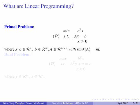
Primal Problem:min cTx
(P) s.t. Ax = bx ≥ 0
where x, c ∈ Rn, b ∈ Rm, A ∈ Rm×n with rank(A) = m.Dual Problem:
max bTx(D) s.t. ATy + s = c
s ≥ 0
where y ∈ Rm, s ∈ Rn.
Voicu, Yang, Zhenghua, Doron (McMaster) Numerical Techniques in IPMs for LP April 2007 3 / 70
What are Linear Programming?
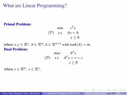
Primal Problem:min cTx
(P) s.t. Ax = bx ≥ 0
where x, c ∈ Rn, b ∈ Rm, A ∈ Rm×n with rank(A) = m.Dual Problem:
max bTx(D) s.t. ATy + s = c
s ≥ 0
where y ∈ Rm, s ∈ Rn.
Voicu, Yang, Zhenghua, Doron (McMaster) Numerical Techniques in IPMs for LP April 2007 3 / 70
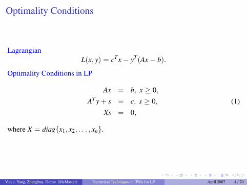
Optimality Conditions
LagrangianL(x, y) = cTx− yT(Ax− b).
Optimality Conditions in LP
Ax = b, x ≥ 0,
ATy + s = c, s ≥ 0, (1)
Xs = 0,
where X = diag{x1, x2, . . . , xn}.
Voicu, Yang, Zhenghua, Doron (McMaster) Numerical Techniques in IPMs for LP April 2007 4 / 70
Outline
1 Introduction of LP
2 Interior Point Method for LPBarrier MethodNewton Direction
3 Solving the Normal Equation SystemThe (Modified) Cholesky FactorizationThe sparse Cholesky Factorization: OrderingsDense Columns in ASymbolic Factorization
4 Solving Augmented System
5 Refinement techniques
Voicu, Yang, Zhenghua, Doron (McMaster) Numerical Techniques in IPMs for LP April 2007 5 / 70
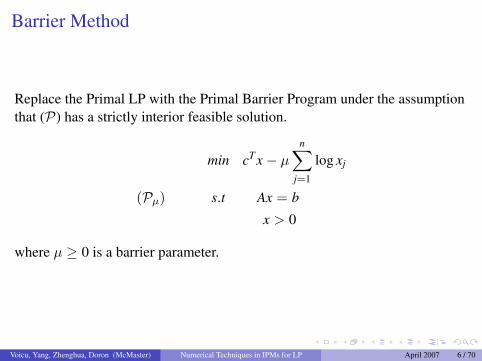
Barrier Method
Replace the Primal LP with the Primal Barrier Program under the assumptionthat (P) has a strictly interior feasible solution.
min cTx− µ
n∑j=1
log xj
(Pµ) s.t Ax = b
x > 0
where µ ≥ 0 is a barrier parameter.
Voicu, Yang, Zhenghua, Doron (McMaster) Numerical Techniques in IPMs for LP April 2007 6 / 70
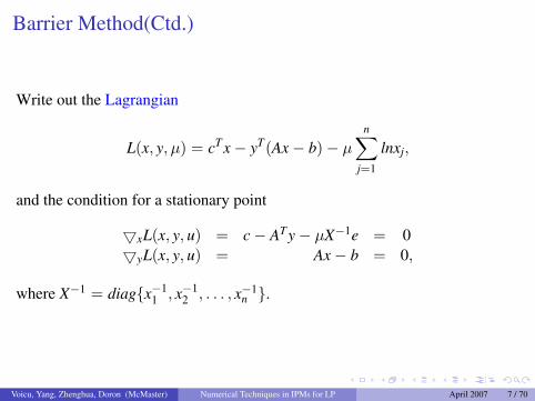
Barrier Method(Ctd.)
Write out the Lagrangian
L(x, y, µ) = cTx− yT(Ax− b)− µ
n∑j=1
lnxj,
and the condition for a stationary point
5xL(x, y, u) = c− ATy− µX−1e = 05yL(x, y, u) = Ax− b = 0,
where X−1 = diag{x−11 , x−1
2 , . . . , x−1n }.
Voicu, Yang, Zhenghua, Doron (McMaster) Numerical Techniques in IPMs for LP April 2007 7 / 70
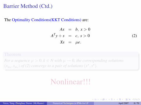
Barrier Method (Ctd.)
The Optimality Conditions(KKT Conditions) are:
Ax = b, x > 0
ATy + s = c, s > 0 (2)
Xs = µe.
TheoremFor a sequence µ > 0, k ∈ N with µ → 0, the corresponding solutions(xµk , sµk) of (2) converge to a pair of solutions (x?, s?).
Nonlinear!!!
Voicu, Yang, Zhenghua, Doron (McMaster) Numerical Techniques in IPMs for LP April 2007 8 / 70
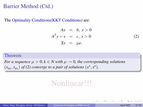
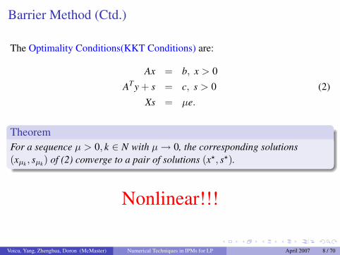
Outline
1 Introduction of LP
2 Interior Point Method for LPBarrier MethodNewton Direction
3 Solving the Normal Equation SystemThe (Modified) Cholesky FactorizationThe sparse Cholesky Factorization: OrderingsDense Columns in ASymbolic Factorization
4 Solving Augmented System
5 Refinement techniques
Voicu, Yang, Zhenghua, Doron (McMaster) Numerical Techniques in IPMs for LP April 2007 9 / 70
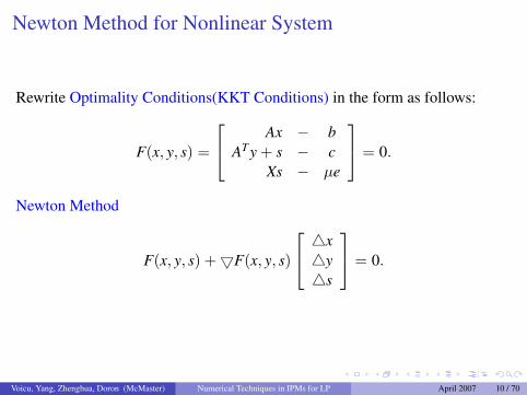
Newton Method for Nonlinear System
Rewrite Optimality Conditions(KKT Conditions) in the form as follows:
F(x, y, s) =
Ax − bATy + s − c
Xs − µe
= 0.
Newton Method
F(x, y, s) +5F(x, y, s)
4x4y4s
= 0.
Voicu, Yang, Zhenghua, Doron (McMaster) Numerical Techniques in IPMs for LP April 2007 10 / 70
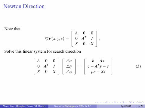
Newton Direction
Note that
5F(x, y, s) =
A 0 00 AT IS 0 X
,
Solve this linear system for search direction A 0 00 AT IS 0 X
4x4y4s
=
b− Axc− ATy− s
µe− Xs
(3)
Voicu, Yang, Zhenghua, Doron (McMaster) Numerical Techniques in IPMs for LP April 2007 11 / 70
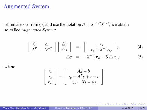
Augmented System
Eliminate 4s from (3) and use the notation D = S−1/2X1/2, we obtainso-called Augmented System:
[0 A
AT −D−2
] [4y4x
]=
[−rb
−rc + X−1rxs
], (4)
4s = −X−1(rxs + S4 x), (5)
where rb
rc
rxs
=
Ax− brc = ATy + s− c
rxs = Xs− µe
Voicu, Yang, Zhenghua, Doron (McMaster) Numerical Techniques in IPMs for LP April 2007 12 / 70
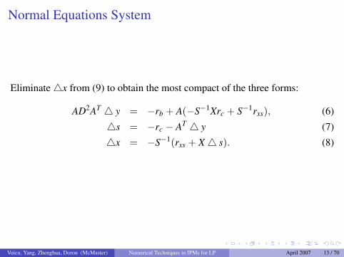
Normal Equations System
Eliminate 4x from (9) to obtain the most compact of the three forms:
AD2AT 4 y = −rb + A(−S−1Xrc + S−1rxs), (6)
4s = −rc − AT 4 y (7)
4x = −S−1(rxs + X 4 s). (8)
Voicu, Yang, Zhenghua, Doron (McMaster) Numerical Techniques in IPMs for LP April 2007 13 / 70
Generic Algorithm
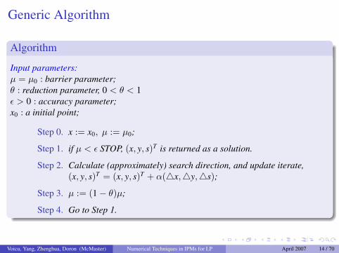
Algorithm
Input parameters:µ = µ0 : barrier parameter;θ : reduction parameter, 0 < θ < 1ε > 0 : accuracy parameter;x0 : a initial point;
Step 0. x := x0, µ := µ0;
Step 1. if µ < ε STOP, (x, y, s)T is returned as a solution.
Step 2. Calculate (approximately) search direction, and update iterate,(x, y, s)T = (x, y, s)T + α(4x,4y,4s);
Step 3. µ := (1− θ)µ;
Step 4. Go to Step 1.
Voicu, Yang, Zhenghua, Doron (McMaster) Numerical Techniques in IPMs for LP April 2007 14 / 70
Outline
1 Introduction of LP
2 Interior Point Method for LPBarrier MethodNewton Direction
3 Solving the Normal Equation SystemThe (Modified) Cholesky FactorizationThe sparse Cholesky Factorization: OrderingsDense Columns in ASymbolic Factorization
4 Solving Augmented System
5 Refinement techniques
Voicu, Yang, Zhenghua, Doron (McMaster) Numerical Techniques in IPMs for LP April 2007 15 / 70
The classical Cholesky Factorization
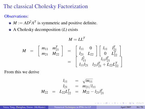
Observations:
M := AD2AT is symmetric and positive definite.
A Cholesky decomposition (L) exists
M = LLT
M =[
m11 mT21
m21 M22
]=
[l11 0l21 L22
] [l11 lT210 LT
22
]=
[l211 l11lT21
l11l21 l21lT21 + L22LT22
]From this we derive
l11 =√
m11l21 = m21/l11
M22 = L22LT22 = M22 − l21lT21
Voicu, Yang, Zhenghua, Doron (McMaster) Numerical Techniques in IPMs for LP April 2007 16 / 70
The classical Cholesky Factorization(Ctd.)
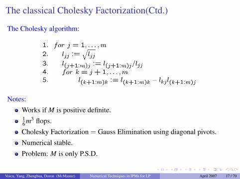
The Cholesky algorithm:
Notes:
Works if M is positive definite.16 m3 flops.
Cholesky Factorization = Gauss Elimination using diagonal pivots.
Numerical stable.
Problem: M is only P.S.D.
Voicu, Yang, Zhenghua, Doron (McMaster) Numerical Techniques in IPMs for LP April 2007 17 / 70
The Modified Cholesky Factorization
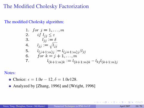
The modified Cholesky algorithm:
Notes:
Choice: ε = 1.0e− 12, δ = 1.0e128.
Analyzed by [Zhang, 1996] and [Wright, 1996]
Voicu, Yang, Zhenghua, Doron (McMaster) Numerical Techniques in IPMs for LP April 2007 18 / 70
Outline
1 Introduction of LP
2 Interior Point Method for LPBarrier MethodNewton Direction
3 Solving the Normal Equation SystemThe (Modified) Cholesky FactorizationThe sparse Cholesky Factorization: OrderingsDense Columns in ASymbolic Factorization
4 Solving Augmented System
5 Refinement techniques
Voicu, Yang, Zhenghua, Doron (McMaster) Numerical Techniques in IPMs for LP April 2007 19 / 70
Fill-in
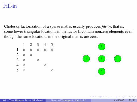
Cholesky factorization of a sparse matrix usually produces fill-in; that is,some lower triangular locations in the factor L contain nonzero elements eventhough the same locations in the original matrix are zero.
1 2 3 4 51 × × × × ×2 × ×3 × ×4 × ×5 × ×
Voicu, Yang, Zhenghua, Doron (McMaster) Numerical Techniques in IPMs for LP April 2007 20 / 70
Fill-in
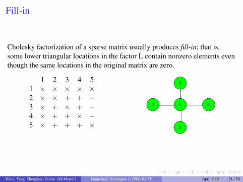
Cholesky factorization of a sparse matrix usually produces fill-in; that is,some lower triangular locations in the factor L contain nonzero elements eventhough the same locations in the original matrix are zero.
1 2 3 4 51 × × × × ×2 × × + + +3 × + × + +4 × + + × +5 × + + + ×
Voicu, Yang, Zhenghua, Doron (McMaster) Numerical Techniques in IPMs for LP April 2007 21 / 70
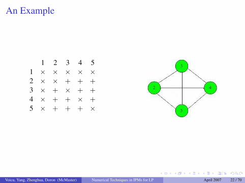
An Example
1 2 3 4 51 × × × × ×2 × × + + +3 × + × + +4 × + + × +5 × + + + ×
Voicu, Yang, Zhenghua, Doron (McMaster) Numerical Techniques in IPMs for LP April 2007 22 / 70
Troubles by fill-in
Disadvantages:
Fill-in requires additional storage.
Fill-in increase the cost of updating the remaining matrix and thetriangular substitutions.
Our Goal: minimizes fill-in
Bad News: NP-complete
Good News: Inexpensive ordering heuristics available
Voicu, Yang, Zhenghua, Doron (McMaster) Numerical Techniques in IPMs for LP April 2007 23 / 70
Minimum-Degree Ordering
Degree: the number of nonzero elements in a column of the matrix,excluding the diagonal.
Motivation: From L22 − l21lT21, we see if l11 has degree d, the update matrixcontains d2 nonzeros.
Process: At each step, examine the remaining matrix and select thediagonal element with minimum degree as the pivot at this step.
Voicu, Yang, Zhenghua, Doron (McMaster) Numerical Techniques in IPMs for LP April 2007 24 / 70

An Example
1 2 3 4 51 × × × × ×2 × ×3 × ×4 × ×5 × ×
Voicu, Yang, Zhenghua, Doron (McMaster) Numerical Techniques in IPMs for LP April 2007 25 / 70
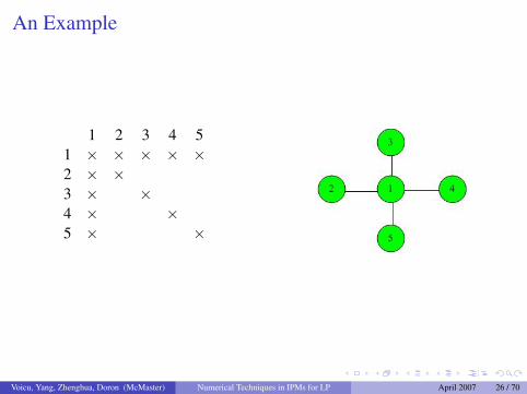
An Example
1 2 3 4 51 × × × × ×2 × ×3 × ×4 × ×5 × ×
Voicu, Yang, Zhenghua, Doron (McMaster) Numerical Techniques in IPMs for LP April 2007 26 / 70
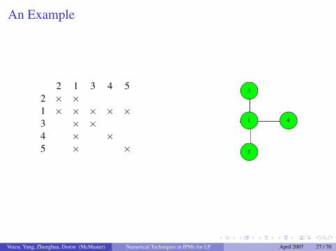
An Example
2 1 3 4 52 × ×1 × × × × ×3 × ×4 × ×5 × ×
Voicu, Yang, Zhenghua, Doron (McMaster) Numerical Techniques in IPMs for LP April 2007 27 / 70
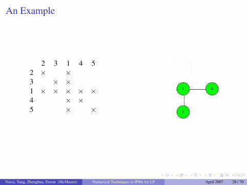
An Example
2 3 1 4 52 × ×3 × ×1 × × × × ×4 × ×5 × ×
Voicu, Yang, Zhenghua, Doron (McMaster) Numerical Techniques in IPMs for LP April 2007 28 / 70
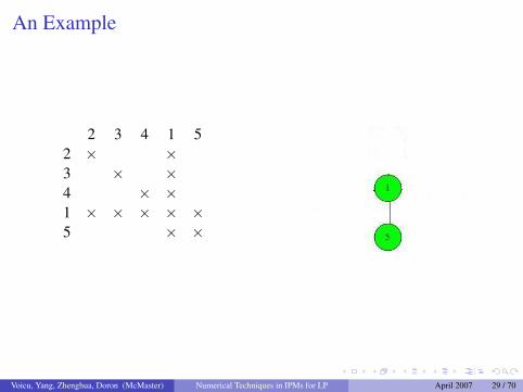
An Example
2 3 4 1 52 × ×3 × ×4 × ×1 × × × × ×5 × ×
Voicu, Yang, Zhenghua, Doron (McMaster) Numerical Techniques in IPMs for LP April 2007 29 / 70
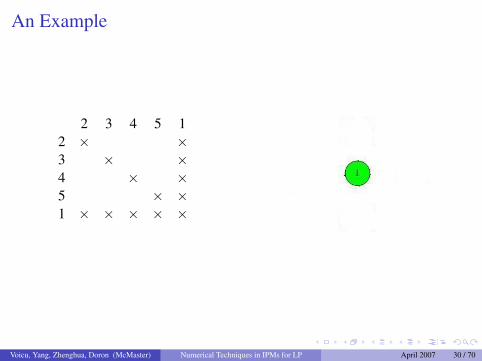
An Example
2 3 4 5 12 × ×3 × ×4 × ×5 × ×1 × × × × ×
Voicu, Yang, Zhenghua, Doron (McMaster) Numerical Techniques in IPMs for LP April 2007 30 / 70
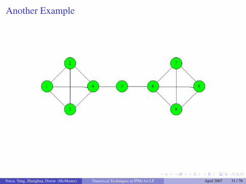
Another Example
Voicu, Yang, Zhenghua, Doron (McMaster) Numerical Techniques in IPMs for LP April 2007 31 / 70
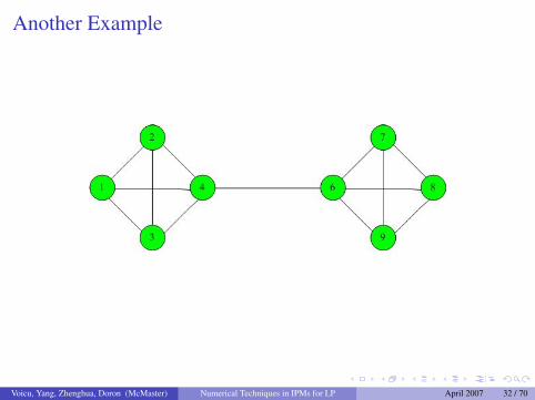
Another Example
Voicu, Yang, Zhenghua, Doron (McMaster) Numerical Techniques in IPMs for LP April 2007 32 / 70
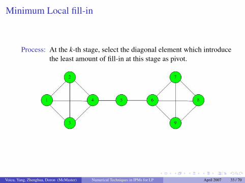
Minimum Local fill-in
Process: At the k-th stage, select the diagonal element which introducethe least amount of fill-in at this stage as pivot.
Voicu, Yang, Zhenghua, Doron (McMaster) Numerical Techniques in IPMs for LP April 2007 33 / 70
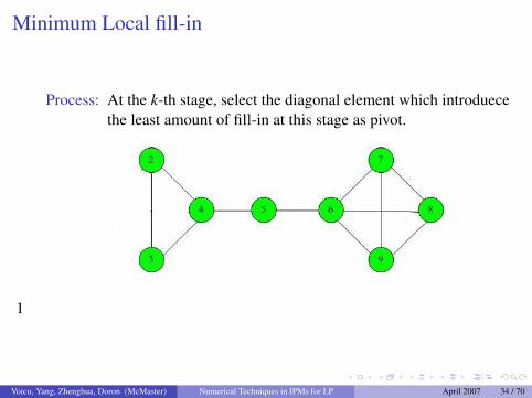
Minimum Local fill-in
Process: At the k-th stage, select the diagonal element which introduecethe least amount of fill-in at this stage as pivot.
1
Voicu, Yang, Zhenghua, Doron (McMaster) Numerical Techniques in IPMs for LP April 2007 34 / 70
Minimum Local fill-in
Process: At the k-th stage, select the diagonal element which introduecethe least amount of fill-in at this stage as pivot.
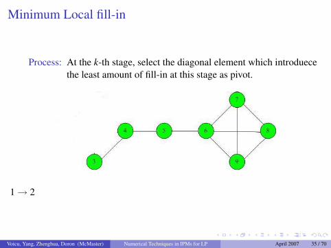
1 → 2
Voicu, Yang, Zhenghua, Doron (McMaster) Numerical Techniques in IPMs for LP April 2007 35 / 70
Minimum Local fill-in
Process: At the k-th stage, select the diagonal element which introduecethe least amount of fill-in at this stage as pivot.
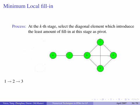
1 → 2 → 3
Voicu, Yang, Zhenghua, Doron (McMaster) Numerical Techniques in IPMs for LP April 2007 36 / 70
Minimum Local fill-in
Process: At the k-th stage, select the diagonal element which introduecethe least amount of fill-in at this stage as pivot.
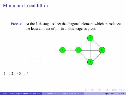
1 → 2 → 3 → 4
Voicu, Yang, Zhenghua, Doron (McMaster) Numerical Techniques in IPMs for LP April 2007 37 / 70
Minimum Local fill-in
Process: At the k-th stage, select the diagonal element which introduecethe least amount of fill-in at this stage as pivot.
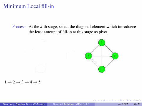
1 → 2 → 3 → 4 → 5
Voicu, Yang, Zhenghua, Doron (McMaster) Numerical Techniques in IPMs for LP April 2007 38 / 70
Minimum Local fill-in
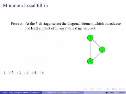
Process: At the k-th stage, select the diagonal element which introduecethe least amount of fill-in at this stage as pivot.
1 → 2 → 3 → 4 → 5 → 6
Voicu, Yang, Zhenghua, Doron (McMaster) Numerical Techniques in IPMs for LP April 2007 39 / 70
Minimum Local fill-in
Process: At the k-th stage, select the diagonal element which introduecethe least amount of fill-in at this stage as pivot.
1 → 2 → 3 → 4 → 5 → 6 → 7
Voicu, Yang, Zhenghua, Doron (McMaster) Numerical Techniques in IPMs for LP April 2007 40 / 70
Minimum Local fill-in
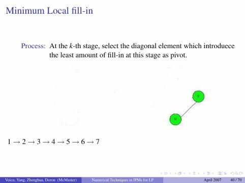
Process: At the k-th stage, select the diagonal element which introduecethe least amount of fill-in at this stage as pivot.
1 → 2 → 3 → 4 → 5 → 6 → 7 → 8
Voicu, Yang, Zhenghua, Doron (McMaster) Numerical Techniques in IPMs for LP April 2007 41 / 70
Minimum Local fill-in
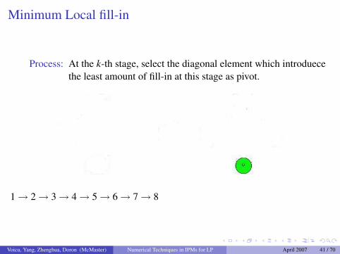
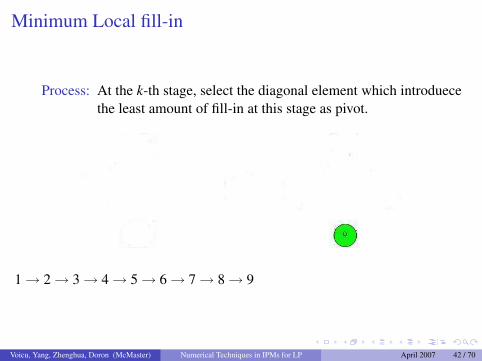
Process: At the k-th stage, select the diagonal element which introduecethe least amount of fill-in at this stage as pivot.
1 → 2 → 3 → 4 → 5 → 6 → 7 → 8 → 9
Voicu, Yang, Zhenghua, Doron (McMaster) Numerical Techniques in IPMs for LP April 2007 42 / 70
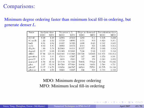
Comparisons:
Minimum degree ordering faster than minimum local fill-in ordering, butgenerate denser L.
MDO: Minimum degree orderingMFO: Minimum local fill-in ordering
Voicu, Yang, Zhenghua, Doron (McMaster) Numerical Techniques in IPMs for LP April 2007 43 / 70
Outline
1 Introduction of LP
2 Interior Point Method for LPBarrier MethodNewton Direction
3 Solving the Normal Equation SystemThe (Modified) Cholesky FactorizationThe sparse Cholesky Factorization: OrderingsDense Columns in ASymbolic Factorization
4 Solving Augmented System
5 Refinement techniques
Voicu, Yang, Zhenghua, Doron (McMaster) Numerical Techniques in IPMs for LP April 2007 44 / 70
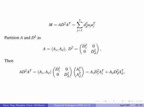
M = AD2AT =n∑
j=1
d2jjajaT
j
Partition A and D2 as
A = (As, Ad), D2 =(
D2s 0
0 D2d
),
Then
AD2AT = (As, Ad)(
D2s 0
0 D2d
) (AT
sAT
d
)= AsD2
s ATs + AdD2
dATd ,
Voicu, Yang, Zhenghua, Doron (McMaster) Numerical Techniques in IPMs for LP April 2007 45 / 70
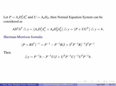
Let P = AsD2s AT
s and U = AdDd, then Normal Equation System can beconsidered as
AD2AT 4 y = (AsD2s AT
s + AdD2dAT
d )4 y = (P + UUT)4 y = b,
Sherman-Morrison formula:
(P + RST)−1 = P−1 − P−1R(I + STP−1R)−1STP−1
Then4y = P−1b− P−1U(I + UTP−1U)−1UTP−1b.
Voicu, Yang, Zhenghua, Doron (McMaster) Numerical Techniques in IPMs for LP April 2007 46 / 70
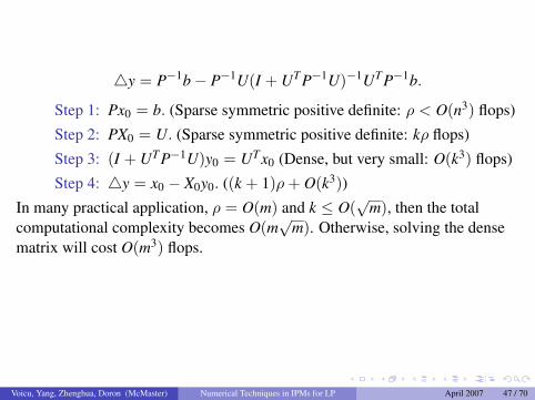
4y = P−1b− P−1U(I + UTP−1U)−1UTP−1b.
Step 1: Px0 = b. (Sparse symmetric positive definite: ρ < O(n3) flops)
Step 2: PX0 = U. (Sparse symmetric positive definite: kρ flops)
Step 3: (I + UTP−1U)y0 = UTx0 (Dense, but very small: O(k3) flops)
Step 4: 4y = x0 − X0y0. ((k + 1)ρ + O(k3))In many practical application, ρ = O(m) and k ≤ O(
√m), then the total
computational complexity becomes O(m√
m). Otherwise, solving the densematrix will cost O(m3) flops.
As may be singular!
Voicu, Yang, Zhenghua, Doron (McMaster) Numerical Techniques in IPMs for LP April 2007 47 / 70
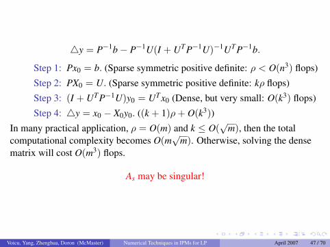
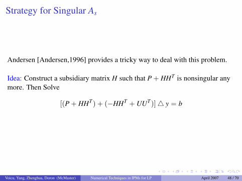
Strategy for Singular As
Andersen [Andersen,1996] provides a tricky way to deal with this problem.
Idea: Construct a subsidiary matrix H such that P + HHT is nonsingular anymore. Then Solve
[(P + HHT) + (−HHT + UUT)]4 y = b
Voicu, Yang, Zhenghua, Doron (McMaster) Numerical Techniques in IPMs for LP April 2007 48 / 70

How to construct H
Apply Gussian Elimination on matrix As to get the upper triangular matrix As.If As is a singular matrix, then there is at least one zero row in As. Assumei1, i2, . . . , im1 , m1 < m, are the indices of zero rows in matrix As. Let
H = (hi1 , hi2 , . . . , him1),
where hk is the k − th unit vector.
Voicu, Yang, Zhenghua, Doron (McMaster) Numerical Techniques in IPMs for LP April 2007 49 / 70
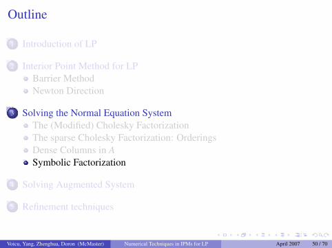
Outline
1 Introduction of LP
2 Interior Point Method for LPBarrier MethodNewton Direction
3 Solving the Normal Equation SystemThe (Modified) Cholesky FactorizationThe sparse Cholesky Factorization: OrderingsDense Columns in ASymbolic Factorization
4 Solving Augmented System
5 Refinement techniques
Voicu, Yang, Zhenghua, Doron (McMaster) Numerical Techniques in IPMs for LP April 2007 50 / 70
What is Symbolic Sparse Cholesky Decomposition?
Cholesky decomposition for positive definite matrices is unconditionallystable1.
It means that we can determine the structure of Choeslky factor withoutactually computing it.
Symbolic decomposition is to compute the sparsity structure of theCholesky decomposition, that is, the locations of the nonzero entries.
Note: 1. G. W. Stewart, Introduction to Matrix Computations, Academic Press Inc., 1973, p.153
Voicu, Yang, Zhenghua, Doron (McMaster) Numerical Techniques in IPMs for LP April 2007 51 / 70
Sparse Matrix Decomposition
Sparse symmetric positive definite matrix can be factorized in two phases:
symbolic decomposition To get the structure of the matrix factor L
numerical decomposition To efficiently compute the numeric values of L andD using the structure determined.
In many sparse matrix programs, these two decompositions are implementedas two separate tasks1.Note: 1. K. H. Law and S. J. Fenives, A node-addition model for symbolic factorization, ACM Trans. Math. Softw. 12 (1986), no. 1, p.37-50
Voicu, Yang, Zhenghua, Doron (McMaster) Numerical Techniques in IPMs for LP April 2007 52 / 70
Advantages of Symbolic Decomposition
To build an efficient data structure to store the nonzero entries of Lbefore computing them
To reduce the time to handle data structure operators during numericalcomputing, so most operations during numerical decomposition arefloat-point operations.
To design efficient numerical decompositions.
Voicu, Yang, Zhenghua, Doron (McMaster) Numerical Techniques in IPMs for LP April 2007 53 / 70
Application on the Implementation of IPM
Iteration 0:I Find sparsity pattern of AAT
I Choose a sparsity preserving orderingI Find sparsity pattern of L
At iteration k:I Form M = ADAT
I Do numerical factorization M.I Do solves.
Voicu, Yang, Zhenghua, Doron (McMaster) Numerical Techniques in IPMs for LP April 2007 54 / 70
Methods of Symbolic Decomposition
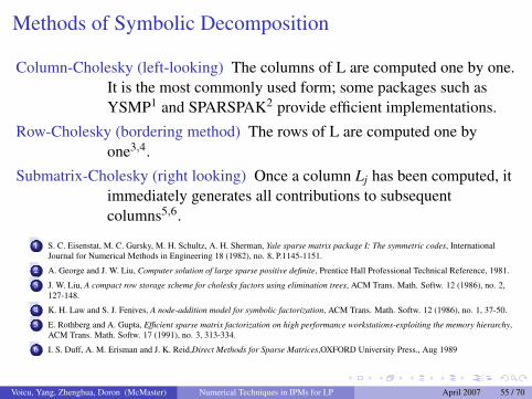
Column-Cholesky (left-looking) The columns of L are computed one by one.It is the most commonly used form; some packages such asYSMP1 and SPARSPAK2 provide efficient implementations.
Row-Cholesky (bordering method) The rows of L are computed one byone3,4.
Submatrix-Cholesky (right looking) Once a column Lj has been computed, itimmediately generates all contributions to subsequentcolumns5,6.
1 S. C. Eisenstat, M. C. Gursky, M. H. Schultz, A. H. Sherman, Yale sparse matrix package I: The symmetric codes, InternationalJournal for Numerical Methods in Engineering 18 (1982), no. 8, P.1145-1151.
2 A. George and J. W. Liu, Computer solution of large sparse positive definite, Prentice Hall Professional Technical Reference, 1981.
3 J. W. Liu, A compact row storage scheme for cholesky factors using elimination trees, ACM Trans. Math. Softw. 12 (1986), no. 2,127-148.
4 K. H. Law and S. J. Fenives, A node-addition model for symbolic factorization, ACM Trans. Math. Softw. 12 (1986), no. 1, 37-50.
5 E. Rothberg and A. Gupta, Efficient sparse matrix factorization on high performance workstations-exploiting the memory hierarchy,ACM Trans. Math. Softw. 17 (1991), no. 3, 313-334.
6 I. S. Duff, A. M. Erisman and J. K. Reid,Direct Methods for Sparse Matrices,OXFORD University Press., Aug 1989
Voicu, Yang, Zhenghua, Doron (McMaster) Numerical Techniques in IPMs for LP April 2007 55 / 70
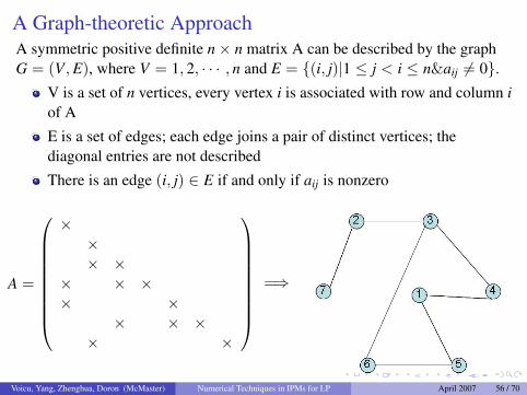
A Graph-theoretic ApproachA symmetric positive definite n× n matrix A can be described by the graphG = (V, E), where V = 1, 2, · · · , n and E = {(i, j)|1 ≤ j < i ≤ n&aij 6= 0}.
V is a set of n vertices, every vertex i is associated with row and column iof A
E is a set of edges; each edge joins a pair of distinct vertices; thediagonal entries are not described
There is an edge (i, j) ∈ E if and only if aij is nonzero
A =
××× ×
× × ×× ×
× × ×× ×
=⇒
Voicu, Yang, Zhenghua, Doron (McMaster) Numerical Techniques in IPMs for LP April 2007 56 / 70
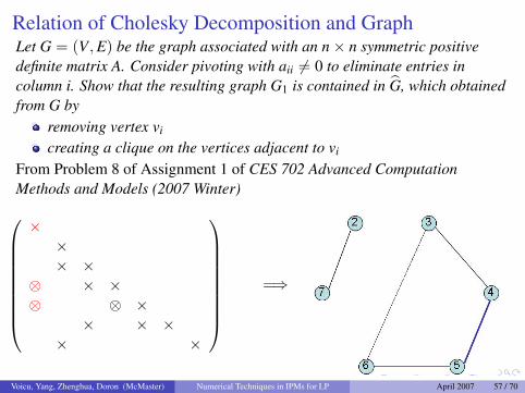
Relation of Cholesky Decomposition and GraphLet G = (V, E) be the graph associated with an n× n symmetric positivedefinite matrix A. Consider pivoting with aii 6= 0 to eliminate entries incolumn i. Show that the resulting graph G1 is contained in G, which obtainedfrom G by
removing vertex vi
creating a clique on the vertices adjacent to vi
From Problem 8 of Assignment 1 of CES 702 Advanced ComputationMethods and Models (2007 Winter)
××× ×
⊗ × ×⊗ ⊗ ×
× × ×× ×
=⇒
Voicu, Yang, Zhenghua, Doron (McMaster) Numerical Techniques in IPMs for LP April 2007 57 / 70
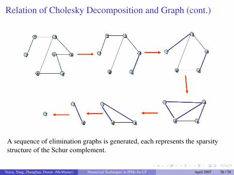
Relation of Cholesky Decomposition and Graph (cont.)
A sequence of elimination graphs is generated, each represents the sparsitystructure of the Schur complement.
Voicu, Yang, Zhenghua, Doron (McMaster) Numerical Techniques in IPMs for LP April 2007 58 / 70
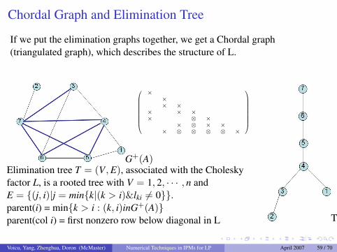
Chordal Graph and Elimination Tree
If we put the elimination graphs together, we get a Chordal graph(triangulated graph), which describes the structure of L.
G+(A)
××× ×
× × ×× ⊗ ×
× ⊗ × ×× ⊗ ⊗ ⊗ ⊗ ×
Elimination tree T = (V, E), associated with the Choleskyfactor L, is a rooted tree with V = 1, 2, · · · , n andE = {(j, i)|j = min{k|(k > i)&lki 6= 0}}.parent(i) = min{k > i : (k, i)inG+(A)}parent(col i) = first nonzero row below diagonal in L T(A)
Voicu, Yang, Zhenghua, Doron (McMaster) Numerical Techniques in IPMs for LP April 2007 59 / 70
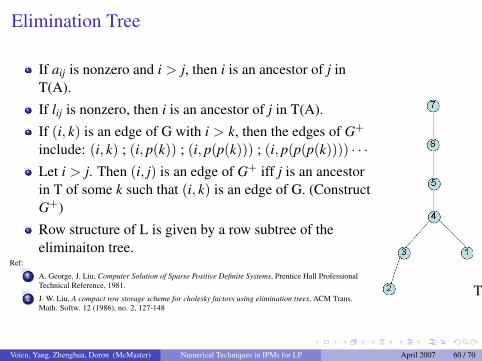
Elimination Tree
If aij is nonzero and i > j, then i is an ancestor of j inT(A).
If lij is nonzero, then i is an ancestor of j in T(A).
If (i, k) is an edge of G with i > k, then the edges of G+
include: (i, k) ; (i, p(k)) ; (i, p(p(k))) ; (i, p(p(p(k)))) · · ·Let i > j. Then (i, j) is an edge of G+ iff j is an ancestorin T of some k such that (i, k) is an edge of G. (ConstructG+)
Row structure of L is given by a row subtree of theeliminaiton tree.
Ref:
1 A. George, J. Liu, Computer Solution of Sparse Positive Definite Systems, Prentice Hall ProfessionalTechnical Reference, 1981.
2 J. W. Liu, A compact row storage scheme for cholesky factors using elimination trees, ACM Trans.Math. Softw. 12 (1986), no. 2, 127-148
T(A)
Voicu, Yang, Zhenghua, Doron (McMaster) Numerical Techniques in IPMs for LP April 2007 60 / 70
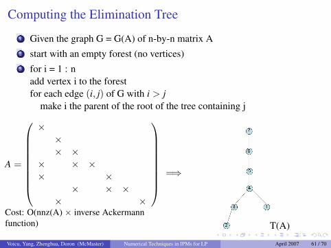
Computing the Elimination Tree
1 Given the graph G = G(A) of n-by-n matrix A2 start with an empty forest (no vertices)3 for i = 1 : n
add vertex i to the forestfor each edge (i, j) of G with i > j
make i the parent of the root of the tree containing j
A =
××× ×
× × ×× ×
× × ×× ×
Cost: O(nnz(A) × inverse Ackermannfunction)
=⇒
T(A)
Voicu, Yang, Zhenghua, Doron (McMaster) Numerical Techniques in IPMs for LP April 2007 61 / 70
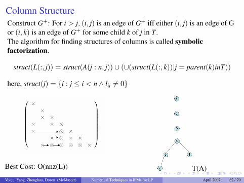
Column StructureConstruct G+: For i > j, (i, j) is an edge of G+ iff either (i, j) is an edge of Gor (i, k) is an edge of G+ for some child k of j in T .The algorithm for finding structures of columns is called symbolicfactorization.
struct(L(:, j)) = struct(A(j : n, j)) ∪ (∪(struct(L(:, k))|j = parent(k)inT))
here, struct(j) = {i : j ≤ i < n ∧ lij 6= 0}
Best Cost: O(nnz(L)) T(A)Voicu, Yang, Zhenghua, Doron (McMaster) Numerical Techniques in IPMs for LP April 2007 62 / 70
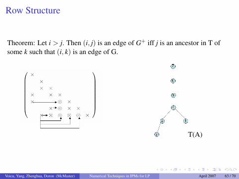
Row Structure
Theorem: Let i > j. Then (i, j) is an edge of G+ iff j is an ancestor in T ofsome k such that (i, k) is an edge of G.
T(A)
Voicu, Yang, Zhenghua, Doron (McMaster) Numerical Techniques in IPMs for LP April 2007 63 / 70
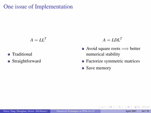
One issue of Implementation
A = LLT A = LDLT
Traditional
Straightforward
Avoid square roots =⇒ betternumerical stability
Factorize symmetric matrices
Save memory
Voicu, Yang, Zhenghua, Doron (McMaster) Numerical Techniques in IPMs for LP April 2007 64 / 70
Software
T. A. Davis, Algorithm 849: A concise sparse cholesky factorizationpackage, ACM Trans. Math. Softw. 31 (2005), no. 4, 587-591.
http://www.cise.ufl.edu/research/sparse/ldl/
Language: C and mex for MatlabTest matrices:
I http://www.cise.ufl.edu/research/sparse/matrices/I http://math.nist.gov/MatrixMarket/
Voicu, Yang, Zhenghua, Doron (McMaster) Numerical Techniques in IPMs for LP April 2007 65 / 70
More Reference of Symbolic Sparse CholeskyDecomposition
Esmond G. Ng,http://www.math.cuhk.edu.hk/NLA2006/EsmondNg.pdf
John Gilbert , Class notes of Sparse Matrix Algorithms, http://www.cs.ucsb.edu/ gilbert/cs290hFall2004/
E. D. Andersen, J. Gondzio, C. M’esz’aros and X. Xu., Implementation of interior-point methods for large-scale linear programming,Technical Report 1996.3, Logilab, HEC Geneva,Section of Management Studies, University of Geneva, Switzerland, 1996
J. W. H. Liu, A generalized envelope method for sparse factorization by rows, ACM Trans. Math. Softw. 17 (1991), no. 1, 112-129.
Voicu, Yang, Zhenghua, Doron (McMaster) Numerical Techniques in IPMs for LP April 2007 66 / 70
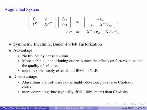
Augmented System[0 A
AT −D−2
] [4y4x
]=
[−rb
−rc + X−1rxs
],
4s = −X−1(rxs + S4 x),
Symmetric Indefinite, Bunch-Parlett FactorizationAdvantage:
I No trouble by dense column.I More stable, ill conditioning easier to trace the effects on factorization and
the quality of solution.I more flexible, easily extended to IPMs in NLP.
Disadvantage:I Algorithms and software not as highly developed as sparse Cholesky
codes.I more computing time (typically, 50%-100% more) than Cholesky.
Voicu, Yang, Zhenghua, Doron (McMaster) Numerical Techniques in IPMs for LP April 2007 67 / 70
Reference
Erling D. Andersen, Jacek Gondzio, Csaba Meszaros, Xiaojie XuImplementtaion of Interior Point Methods for Large Scale Linear Programmingin Iterior point methods of mathematical programming Edited by Tamaas Terlaky, Kluwer, 1996
E.D. Andersen, C. Roos, T. Terlaky, T. Trafalis, and J.P. Warners.The use of low-rank updates in interior-point methods.Technical Report, Delft University of Technology, The Netherlands, 1996.
E.D. Andersen and K.D. AndersonThe Mosek Interior point Optimizer for Linear Programming: An Implementation of the Homogeneous AlgorithmIn H. Frenk , C. Roos, T. Terlaky and S. Zhang (Editors), High Performance Optimization, Kluwer Academic Publishers, Boston,197-232, 1999.
K.D. AndersenA Modified Schur Complement Method for Handling Dense Columns in Interior-Point Methods for Linear Programming.ACM Trans. Math. Software, 22(3), 348-356, 1996.
I.S. Duff A.M. Erisman J.K. ReidDirect Methods for Sparese MatricesClearendon Press, Xoford, 1986
Alan George, Joseph W-H LiuComputer Solution of Large Sparse Positive Definite SystemsPrentice-Hall, Inc. Enlewood Cliffs, new Jeersey, 1981.
Voicu, Yang, Zhenghua, Doron (McMaster) Numerical Techniques in IPMs for LP April 2007 68 / 70
Reference
W.W. HagerUpdating the inverse of a matrixSIAM Rev., 31(2), 221-239, 1989.
B. Jansen, C. Roos, T. TerlakyA short survey on ten years interior point methodsTechnical Report 95-45, Delft University of Technology, Netherlands.
S.J. WrightModified Cholesky factorizations in interior-point algorithms for linear programming,Preprint ANL/MCS-P600-0596, Mathematics and Computer Science Division, Argonne National Laboratory, Argonne, ILL, May1996.
Yin ZhangSolving Large-Scale Linear Programs by Interior-Point Methods Under the MATLAB EnvironmentDepartment of Mathematics and Statistics, University of Maryland Baltimore County, Technical Report TR96-01
Voicu, Yang, Zhenghua, Doron (McMaster) Numerical Techniques in IPMs for LP April 2007 69 / 70
Thanks!
Questions?
Voicu, Yang, Zhenghua, Doron (McMaster) Numerical Techniques in IPMs for LP April 2007 70 / 70