numerical simulation of compaction and subsidence · pdf file2006 abaqus users’...

2006 ABAQUS Users’ Conference 125

Numerical Simulation of Compaction and Subsidence Using ABAQUS

Gaia Capasso and Stefano Mantica

Eni S.p.A., Exploration and Production Division, Milan (Italy)

Abstract: The evaluation of reservoir compaction and surface subsidence induced by hydrocarbon production represents a critical concern to oil companies and government environmental agencies. In this paper, we present an approach to evaluate strain and deformations at reservoir scale by using ABAQUS, linked to the flow simulator used in Eni E&P. Keywords: Reservoir Compaction, Surface Subsidence, Environment, Cam-Clay, Geomechanics, Hydrocarbon Production.

1. Introduction

The study of hydrocarbon production from an underground reservoir involves two basic elements: the rock and the fluid contained in its pore space. Fluid flow and fluid pressure evolution together with stress-strain variation in the solid skeleton are the processes associated with the exploitation of the field. Fluid flow analysis is essential in any reservoir study in order to forecast the production and manage the development of the field; nonetheless, the geomechanical processes associated with the reservoir exploitation are also of primary interest, since they can affect the behaviour of the reservoir itself and cause environmental impact as a consequence of productive layer compaction and land subsidence. Then, the evaluation of reservoir compaction and surface subsidence induced by hydrocarbon production represents a critical concern to oil companies and government environmental agencies.

Reservoir compaction may alter the rock permeability over time with a consequent reduction in well rates, a delay in reserves recovery and a decrease in ultimate recovery from compaction-drive reservoirs (Ostermeier, 1995). In this case, a reliable forecast of the compaction is required for an optimized management of reservoir production. Moreover, the accurate prediction of soil deformation is crucial for the design of casing and completion to avoid well failures induced by high levels of compaction (da Silva, 1990; Bruno, 1992). In addition, surface subsidence that may be induced by hydrocarbon production must be considered in the design of surface facilities or to prevent adverse environmental impact when the reservoir is located close to an area of ecological, historical or social significance.

126 2006 ABAQUS Users’ Conference

Surface subsidence and reservoir compaction due to hydrocarbon production have been documented for fields located in many different areas in the world, from the North Sea to the United States and South America. Subsidence at the Ekofisk oil field (North Sea) is widely known because of its absolute magnitude, of the order of meters (Zaman, 1995); in the Netherlands, subsidence at the Groningen gas field, though only of the order of tens of centimeters, is of great significance since large areas of the Netherlands are below sea level (Boot, 1973).

In Italy, interest has increased during recent years because of the exploitation of the gas fields located off-shore in the Adriatic Sea; as a consequence, advanced methodologies have been developed internally in Eni E&P in order to study the problem of reservoir compaction, to fully understand the mechanisms involved in surface subsidence and to forecast and prevent adverse environmental impacts.

In this paper, we present a procedure to evaluate stress and strain at reservoir scale by using ABAQUS, linked to the flow simulator Eclipse (Schlumberger, 2004) used in Eni E&P. First, we give a description of the problem and of the general methodology by providing an overview of the workflow that has been developed. Next, we illustrate the application of this approach to a realistic test case. Finally, we conclude with a discussion on the obtained results and the perspective for future work.

2. Problem description

Rock compaction and the associated subsidence, i.e. the sinking or settlement of the land surface, may occur due to hydrocarbon withdrawal from the subsurface.

Considering the reservoir as a porous medium, the basic mechanism controlling compaction and subsidence phenomena can be explained referring to Terzaghi’s principle of effective stress, which governs the interaction between solid skeleton and fluid, stating that:

pijijij δσσ −='

where σij’ is the effective stress, σij is the total stress, and p is the pore pressure. The effective stress governs the mechanical behaviour of the porous medium since “all measurable effects of a change of stress, such as compression, distortion and a change of shearing resistance, are exclusively due to changes in the effective stress” (Terzaghi, 1936).

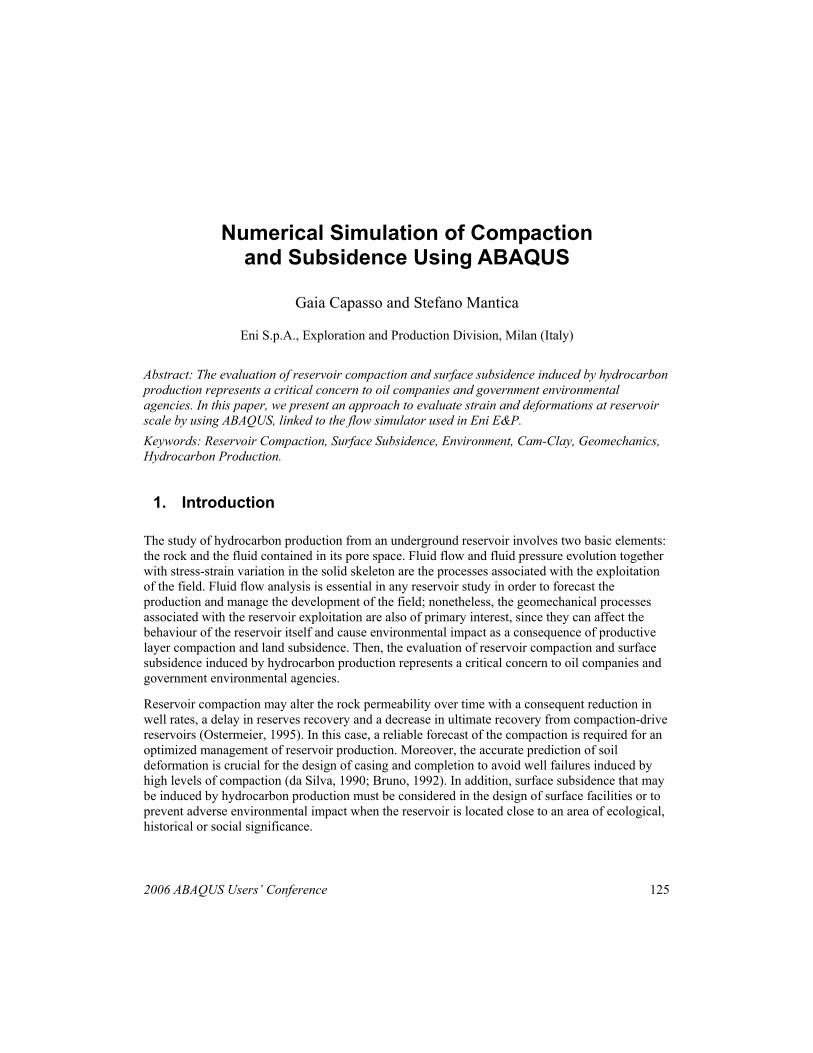
With reference to a reservoir, the above principle can be applied by considering that the weight of the overburden is supported partially by the rock matrix and partially by the pressurized fluid in its pore space; the reduction of the pore pressure due to reservoir exploitation will induce an increase of the effective stress with a consequent compaction effect on the formation (Figure 1).


start production end production

pp11pp11 pp22pp22

CompactionCompaction

SubsidenceSubsidence

Reservoir pore-pressure

Effective stress

reservoir p2 < p1

Figure 1 – Compaction and subsidence due to reservoir exploitation.

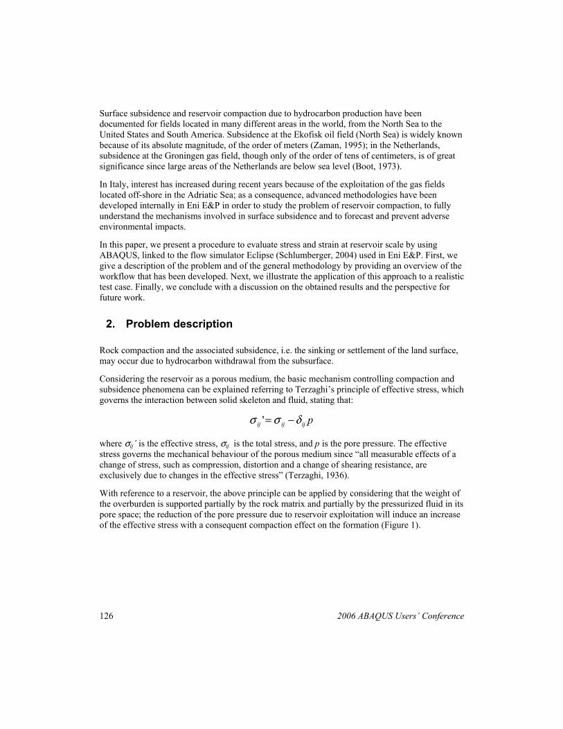
In order to study the phenomenon, analytical and semi-analytical methods have been developed in the past. One of the simplest approaches that allows for the quantitative determination of surface subsidence due to the depletion of a reservoir, as well as the deformation of the whole half-space surrounding the reservoir itself, is Geertsma’s analytical solution (Geertsma, 1973), based on the concept of the “nucleus of strain” (Mindlin, 1950). This approach, however, is valid under a number of simplifying hypotheses, which are usually not respected in a real case: cylindrical shape of the reservoir, uniform depletion, linear elastic behaviour and homogeneity of the porous medium (Figure 2, left). Some of these hypotheses can be overcome by using a semi-analytical approach based on the same concept (Geertsma, 1973a); in this case the discretization of the depleting volume allows for a more realistic description of the reservoir geometry and depletion distribution (Figure 2, right).

Land surfaceLand surface Land surfaceLand surfaceLand surfaceLand surface

Figure 2 – Analytical (left) and semi-analytical Geertsma approaches.


However, the semi-analytical approach is still limited because of the hypotheses of linear elastic homogeneous material. The homogeneity of the material means that the model is forced to describe the whole medium, i.e. reservoir, side-, over- and under-burden, with the same mechanical properties. Decreasing compressibility usually occurring with increasing depth, as well as different characterization of various lithologies cannot be taken into account. The hypothesis of linear elastic behaviour imposes the same linear relationship between stress and strain, both during loading (depletion) and unloading (repressurization); on the contrary, it is known that the soil can have a highly non linear behaviour, with a strong influence of previous stress paths.

In many cases, the use of a finite element (FE) model is than much more suitable in order to fully describe the geomechanical behaviour of a depleting reservoir and of the surrounding material. It is possible, in this case, to build an FE model with a detailed description of the geometry, taking into account the geological structure of the producing layers and of the over- and under-burden layers; regions with different mechanical properties and complex constitutive laws can be defined in order to correctly consider the behaviour of the materials; the system can be loaded with the measured drawdown which is function of space and time. A workflow has been developed internally in Eni E&P by using ABAQUS as the main numerical tool for geomechanical simulations.

3. Reservoir modeling

The results of the standard reservoir studies carried out for the management of the field production provide part of the inputs necessary for a geomechanical finite element analysis. The typical workflow of a reservoir study consists of a “static” study and a “dynamic” study.

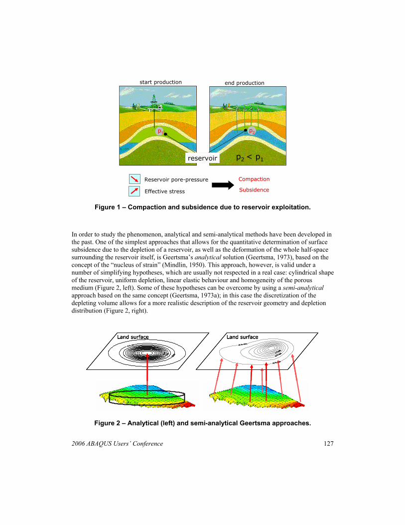
The “static” model includes the detailed reconstruction of the geological structure of the reservoir (e.g. the shape of the layers and the trend of the faults), the definition of the mineralized volumes and the attribution of the petrophysical parameters (initial porosity and permeability) as a function of the location. The result of a static study is a 3D model of the reservoir and of the surrounding region, describing all its geological, lithological, stratigraphical and petrophysical aspects. Figure 3 shows, as an example, the geometry of the top of a gas field layer, where all the faults present in the area are reported.


Figure 3 – 3D static model: representation of a geological horizon and faults.

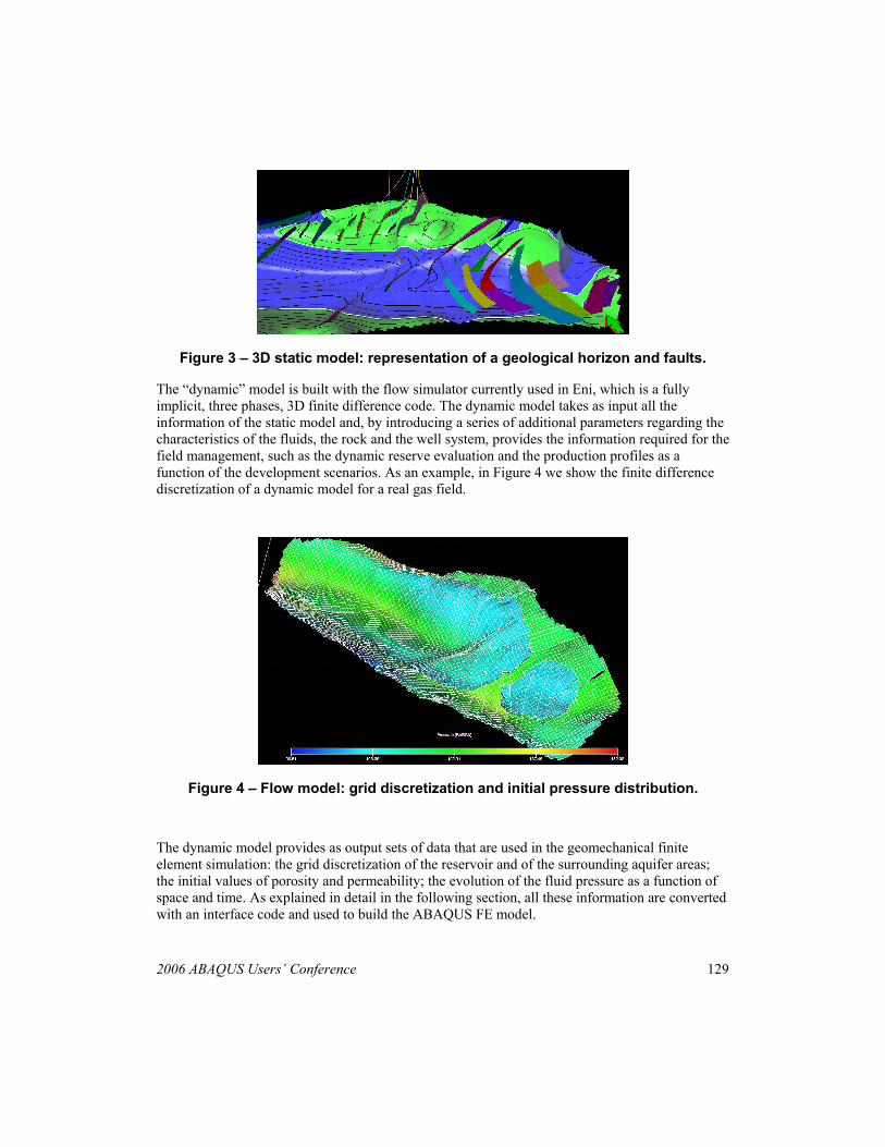
The “dynamic” model is built with the flow simulator currently used in Eni, which is a fully implicit, three phases, 3D finite difference code. The dynamic model takes as input all the information of the static model and, by introducing a series of additional parameters regarding the characteristics of the fluids, the rock and the well system, provides the information required for the field management, such as the dynamic reserve evaluation and the production profiles as a function of the development scenarios. As an example, in Figure 4 we show the finite difference discretization of a dynamic model for a real gas field.

Figure 4 – Flow model: grid discretization and initial pressure distribution.

The dynamic model provides as output sets of data that are used in the geomechanical finite element simulation: the grid discretization of the reservoir and of the surrounding aquifer areas; the initial values of porosity and permeability; the evolution of the fluid pressure as a function of space and time. As explained in detail in the following section, all these information are converted with an interface code and used to build the ABAQUS FE model.


4. Subsidence studies workflow

A workflow has been developed in Eni E&P in order to carry out geomechanical simulations with the FE code ABAQUS; the aim is to assess the stress/strain evolution of the field and of the surrounding rock during the productive life of the reservoir and after the abandonment. The compaction of the depleting layers as well as the evolution of surface subsidence can then be quantitatively evaluated.

The workflow includes the following steps:

1. Model construction: a FE grid for the reservoir region is built starting from the FD (Eclipse) discretization; the FE grid is then enlarged in order to include over-, under and side-burden; the FE model is created and populated with the reservoir data derived by the flow model;

2. Linear elastic simulations: FE simulations under linear elastic hypotheses are carried out and compared to a reference semi-analytical solution in order to validate the gridding, the boundary conditions and the pressure attribution at the finite element nodes;

3. Elasto-plastic simulations: FE simulations using realistic constitutive behaviour (elasto-plasticity) and appropriate description of the heterogeneity of the materials are performed including all the information available for the field.

4.1 Model construction

A Fortran90 interface code that provides an automated link between the flow model and ABAQUS has been developed in-house: files with the results of the flow simulation are processed and the needed information is re-written as input files to run ABAQUS.

The geometrical information of the Eclipse 3D corner point grid are directly extracted from the relevant output files of the flow model and processed to build the FE mesh in the reservoir region. This approach allows for the definition of a FE model which is fully consistent with the reservoir FD model.

The typical FD and FE grid structures are shown in Figure 5 for a 2D mesh.


F.E.M.F.E.M. GRIDGRID

Node #

1 x, y… …12 x, y

Coords

Element # Node #

1 1 2 6 5… …6 7 8 12 11

F.E.M.F.E.M. GRIDGRID

Node #

1 x, y… …12 x, y

Coords

Element # Node #

1 1 2 6 5… …6 7 8 12 11

Element # Node #

1 1 2 6 5… …6 7 8 12 11

F.D.F.D. GRIDGRID

Cell

(1,1) (x1,y1)…(x4,y4)(2,1) (x1,y1)…(x4,y4)

… …(2,3) (x1,y1)…(x4,y4)

Node coords

F.D.F.D. GRIDGRID

Cell

(1,1) (x1,y1)…(x4,y4)(2,1) (x1,y1)…(x4,y4)

… …(2,3) (x1,y1)…(x4,y4)

Node coords

o o o o

o o o o

o o o o

j=1 j=2 j=3

i=1

i=2

1 2 3 4

5 6 7 8

9 10 11 12

1 2 3

4 5 6

o o o o

o o o o

o o o o

j=1 j=2 j=3

i=1

i=2

j=1 j=2 j=3

i=1

i=2

1 2 3 4

5 6 7 8

9 10 11 12

1 2 3

4 5 6

Figure 5 - From FD to FE grid.

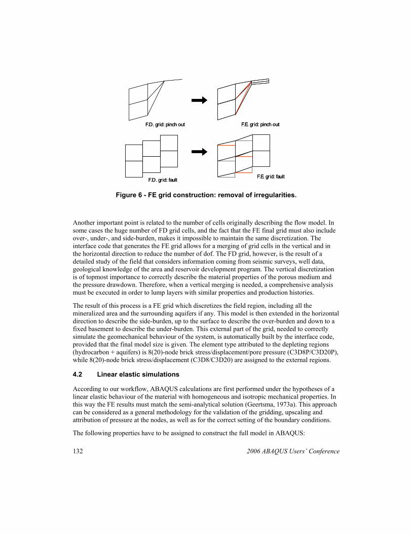
It has to be noted that the FD mesh is built according to the geological structure of the reservoir, i.e. stratigraphy and fault geometries are respected as much as possible. This may produce a series of geometrical “irregularities” that are allowed in FD simulations but cannot be straightly maintained in a FE grid. In order to describe the real geometry of soil levels with vanishing thickness (“pinch-outs”), some cells in the FD grid may have nodes collapsing in a single point; the presence of faults, in addition, is often described in a FD grid with its real dislocation, causing the shift between nodes of two neighboring cells. Small irregularities are removed during the grid processing by slightly adjusting the node position in order to get a suitable FE grid without losing the correct geological structure (see Figure 6).


F.D. grid: pinch out F.E. grid: pinch outF.D. grid: pinch out F.E. grid: pinch out

F.D. grid: fault F.E. grid: faultF.D. grid: fault F.E. grid: fault

Figure 6 - FE grid construction: removal of irregularities.

Another important point is related to the number of cells originally describing the flow model. In some cases the huge number of FD grid cells, and the fact that the FE final grid must also include over-, under-, and side-burden, makes it impossible to maintain the same discretization. The interface code that generates the FE grid allows for a merging of grid cells in the vertical and in the horizontal direction to reduce the number of dof. The FD grid, however, is the result of a detailed study of the field that considers information coming from seismic surveys, well data, geological knowledge of the area and reservoir development program. The vertical discretization is of topmost importance to correctly describe the material properties of the porous medium and the pressure drawdown. Therefore, when a vertical merging is needed, a comprehensive analysis must be executed in order to lump layers with similar properties and production histories.

The result of this process is a FE grid which discretizes the field region, including all the mineralized area and the surrounding aquifers if any. This model is then extended in the horizontal direction to describe the side-burden, up to the surface to describe the over-burden and down to a fixed basement to describe the under-burden. This external part of the grid, needed to correctly simulate the geomechanical behaviour of the system, is automatically built by the interface code, provided that the final model size is given. The element type attributed to the depleting regions (hydrocarbon + aquifers) is 8(20)-node brick stress/displacement/pore pressure (C3D8P/C3D20P), while 8(20)-node brick stress/displacement (C3D8/C3D20) are assigned to the external regions.

4.2 Linear elastic simulations

According to our workflow, ABAQUS calculations are first performed under the hypotheses of a linear elastic behaviour of the material with homogeneous and isotropic mechanical properties. In this way the FE results must match the semi-analytical solution (Geertsma, 1973a). This approach can be considered as a general methodology for the validation of the gridding, upscaling and attribution of pressure at the nodes, as well as for the correct setting of the boundary conditions.

The following properties have to be assigned to construct the full model in ABAQUS:


• bulk density ρ (elements C3D8) and dry density ρd=ρ-φ.γf/g (elements C3D8P); elasticity modulus E and Poisson ratio ν;

• specific weight of the pore fluid γf (elements C3D8P);

• initial void ratio e=φ/(1-φ) (elements C3D8P);

• tabulated values of permeability vs. void ratio (elements C3D8P).

Note that density, initial void ratio and permeability do not affect the result of elastic simulations.

A sensitivity study is then carried out on different grids by possibly varying the number of elements modeling the over-, under- and side-burden; the extent of the model itself; and, finally, the element merging procedure.

The results of the ABAQUS models are compared with the semi-analytical solution: the final grid structure is chosen to be the one that best reproduces the semi-analytical solution with the minimum computational effort.

4.3 Elasto-plastic simulations

Once the geometry of the model has been defined in terms of size and discretization, the final FE model is built with constitutive laws and material properties according to the available data.

In this section we introduce the criteria used for the definition of the hydro-mechanical regions and the evaluation of the material properties associated to them. Next, the definition of the initial state is described in terms of stress condition, pore pressure equilibrium and initial void ratio.

4.3.1 Region definition

The FE geomechanical model, as already discussed in §4.1, is built by considering two different classes of elements. It comprises porous elements corresponding to the fluid saturated zones of the flow model and non-porous elements corresponding to over-, under- and side-burden.

The region definition in the non-porous zone depends on the distribution of the mechanical properties and, in particular, on its heterogeneity. In the fluid saturated zones, as a general rule, each layer constitutes a region: the layering of the flow model, which is preserved in the FE model, is in fact generated by taking into account the real stratigraphy of the reservoir.

For each porous layer a further region subdivision is necessary if a fluid-fluid contact is present. This permits to account for different fluids with different properties and behaviour into the single phase ABAQUS simulator. Thence, each porous layer is split into up to three regions (gas, oil and water) defined by the relevant contact depth.

4.3.2 Material properties

Density


The density is given in the FE model as a function of depth. Since this option is not directly available in ABAQUS, the following simple approach has been adopted: the variable temperature is introduced in the model as an initial condition with values corresponding to the node depth, so that the density can be assigned as a function of temperature. This is of course a strong restriction because it makes impossible the use of the temperature as a physical variable.

The bulk density profile ρ(z) is usually obtained from sonic and density logs measured along the wells; in the non-porous regions it is provided in a tabular form as a function of depth, while in the porous regions the dry density ρd of the material has to be entered, which is defined as:

gf

d

γφρρ

⋅−=

being φ the region porosity, g the gravity acceleration and γf the specific weight of the saturating fluid. For each porous region the dry density is then provided as function of depth.

Fluid specific weight

In the porous regions, the specific weight of the saturating fluid has to be provided. For each hydro-mechanical region the value of γf (gas, oil or water) is taken as constant; it is determined as an average value by using the fluid contact depths and the initial pressure distribution of the region as calculated by the flow model.

Constitutive law

Depending on the material characterizing the reservoir and the surrounding zones, the most appropriate behaviour is used in the model, by choosing among the elasto-plastic constitutive laws implemented in ABAQUS for geomaterials. Usually, the Modified Cam Clay model is used in the case of sandy/shaly materials, while models based on strength criterions (Mohr-Coulomb, Drucker-Prager) are preferred when dealing with limestone or dolomite. The property values needed for the law definition are derived by laboratory or in situ tests.

4.3.3 Initialization

Stress

The stress initialization is a critical point when using elasto-plastic constitutive laws, since the material behaviour is controlled by the current value of the stress and by its path, not only by the stress variations.

The stress initialization is performed through the following steps:

• an initial in situ stress field is computed using the material density ρ(z) and a K0 value (the ratio between horizontal and vertical stress) obtained from in situ measurements of horizontal stress available for the field;

• the model is then equilibrated with this stress field as initial condition, assuming linear elastic behaviour of the material and using the *GEOSTATIC option to verify that the


geostatic stress field is in equilibrium with the applied loads and boundary conditions on the model and to iterate, if needed, to obtain equilibrium;

• the resulting stress field is then used to initialize the elasto-plastic simulation;

• a further *GEOSTATIC step is performed at the start of the elasto-plastic simulation in order to verify that negligible displacements occur.

The correct attribution of the initial stress is a crucial step since the initial geometry should not be changed by the initialization process, being known as it is at the beginning of production.

Void ratio

The initial void ratios e, assigned to the porous regions of the ABAQUS model, are assumed constant region by region and are obtained by averaging the initial porosity values of the flow simulation.

Pore pressure

The initial pore pressure field is given as calculated by the flow model initialization, then consistently with the fluid contacts and with the specific weight of the saturating fluids.

4.3.4 Boundary conditions

The boundary conditions assigned to the model consist of null displacement at the bottom of the grid and no horizontal displacement at the sides. Step 2 of the workflow assures that the mesh is sufficiently extended so that the boundary conditions imposed do not affect the simulation results.

4.3.5 Load history

The pressure time evolution is automatically extracted from the flow model output files at the time steps of interest and re-written in order to be directly available as ABAQUS input.

It must be noted that pressure is cell centered in the FD flow simulation, while it is node centered in the ABAQUS simulator. The pore pressure Pi at each node i of the FE grid is then obtained as a weighted average of the cell centered pressures pj of the FD simulation as follows:

( ) ( )

( )∑∑

=

=

⋅=

8,1

8,1

jj

jjj

i iporv

iporvipP

where the j sum runs over the 8 neighboring cells sharing node i, characterized by pressure pj(i) and pore volume porvj(i).

The pressure values obtained with this processing are then applied as boundary conditions at each step of the FE ABAQUS calculation, providing the load history of the model.


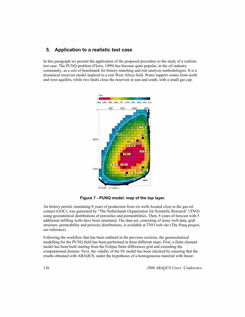
5. Application to a realistic test case

In this paragraph we present the application of the proposed procedure to the study of a realistic test case. The PUNQ problem (Floris, 1999) has become quite popular, in the oil industry community, as a sort of benchmark for history matching and risk analysis methodologies. It is a dynamical reservoir model inspired to a real West Africa field. Water support comes from north and west aquifers, while two faults close the reservoir at east and south, with a small gas cap.

Figure 7 - PUNQ model: map of the top layer.

An history period, simulating 8 years of production from six wells located close to the gas-oil contact (GOC), was generated by “The Netherlands Organization for Scientific Research” (TNO) using geostatistical distributions of porosities and permeabilities. Then, 8 years of forecast with 5 additional infilling wells have been simulated. The data-set, consisting of noisy well-data, grid structure, permeability and porosity distributions, is available at TNO web site (The Punq project, see reference).

Following the workflow that has been outlined in the previous sections, the geomechanical modelling for the PUNQ field has been performed in three different steps. First, a finite element model has been built starting from the Eclipse finite differences grid and extending the computational domain. Next, the validity of the FE model has been checked by ensuring that the results obtained with ABAQUS, under the hypotheses of a homogeneous material with linear-


elastic behaviour, and the semi-analytical solution be equivalent. Finally, one-way coupled poro-elasto-plastic simulations based on the Cam-Clay material behaviour have been performed.

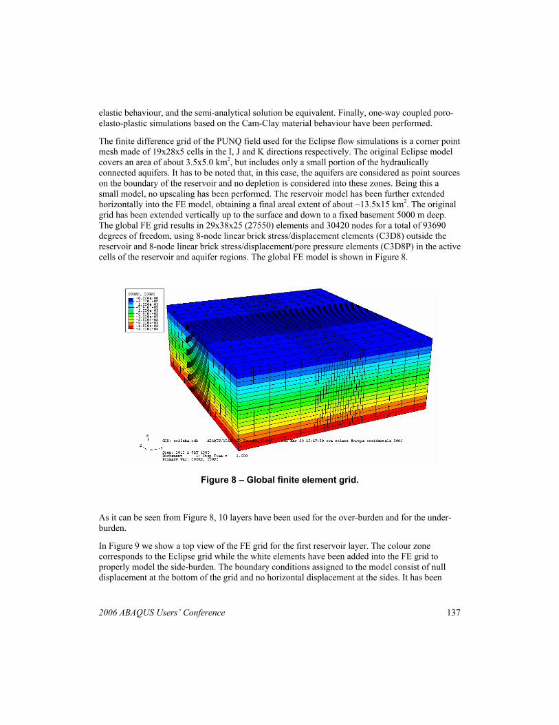
The finite difference grid of the PUNQ field used for the Eclipse flow simulations is a corner point mesh made of 19x28x5 cells in the I, J and K directions respectively. The original Eclipse model covers an area of about 3.5x5.0 km2, but includes only a small portion of the hydraulically connected aquifers. It has to be noted that, in this case, the aquifers are considered as point sources on the boundary of the reservoir and no depletion is considered into these zones. Being this a small model, no upscaling has been performed. The reservoir model has been further extended horizontally into the FE model, obtaining a final areal extent of about ~13.5x15 km2. The original grid has been extended vertically up to the surface and down to a fixed basement 5000 m deep. The global FE grid results in 29x38x25 (27550) elements and 30420 nodes for a total of 93690 degrees of freedom, using 8-node linear brick stress/displacement elements (C3D8) outside the reservoir and 8-node linear brick stress/displacement/pore pressure elements (C3D8P) in the active cells of the reservoir and aquifer regions. The global FE model is shown in Figure 8.

Figure 8 – Global finite element grid.

As it can be seen from Figure 8, 10 layers have been used for the over-burden and for the under-burden.

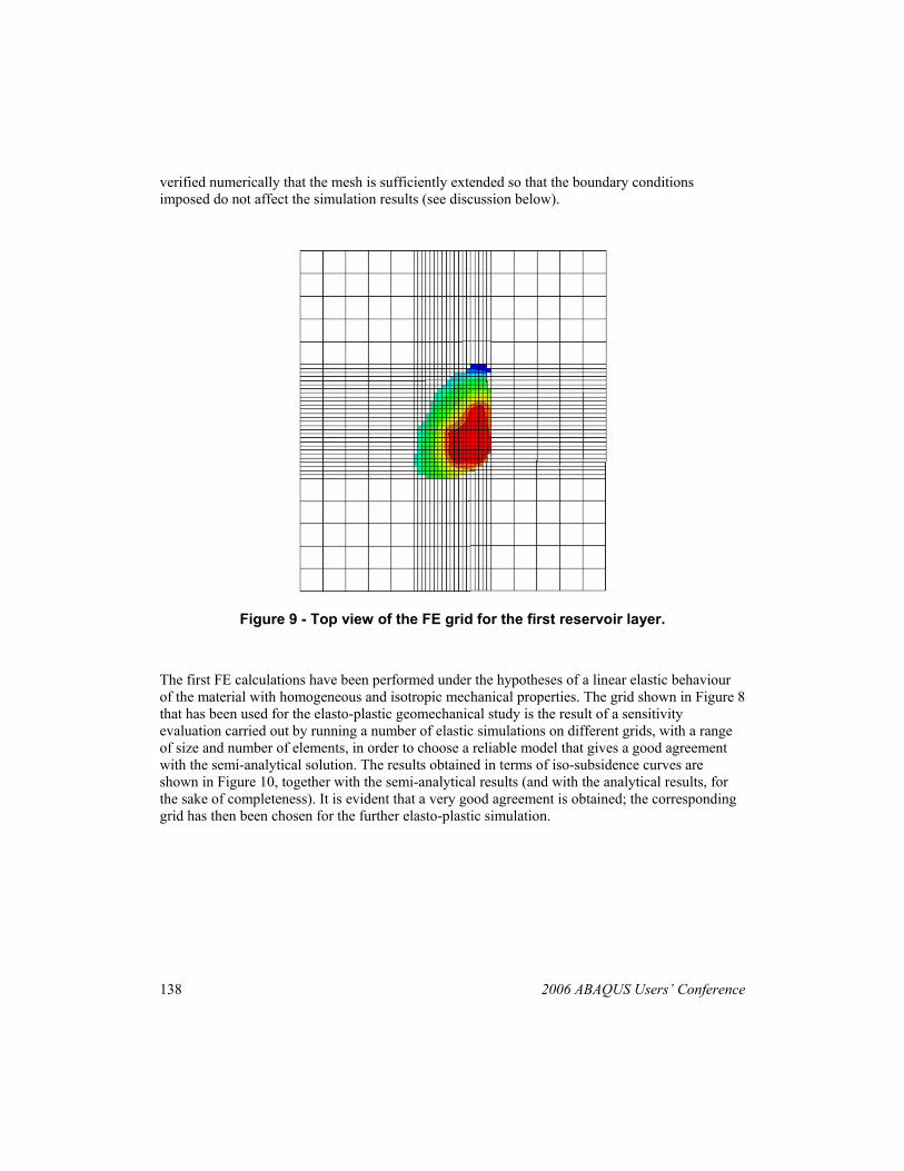
In Figure 9 we show a top view of the FE grid for the first reservoir layer. The colour zone corresponds to the Eclipse grid while the white elements have been added into the FE grid to properly model the side-burden. The boundary conditions assigned to the model consist of null displacement at the bottom of the grid and no horizontal displacement at the sides. It has been


verified numerically that the mesh is sufficiently extended so that the boundary conditions imposed do not affect the simulation results (see discussion below).

Figure 9 - Top view of the FE grid for the first reservoir layer.

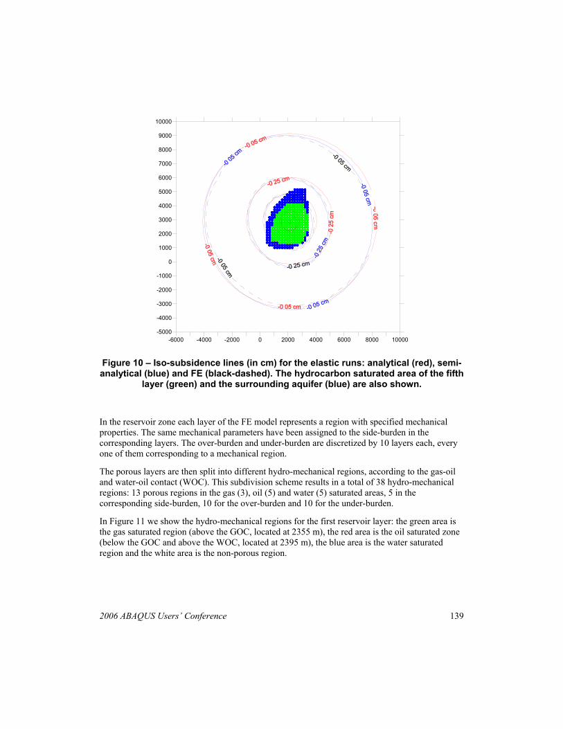
The first FE calculations have been performed under the hypotheses of a linear elastic behaviour of the material with homogeneous and isotropic mechanical properties. The grid shown in Figure 8 that has been used for the elasto-plastic geomechanical study is the result of a sensitivity evaluation carried out by running a number of elastic simulations on different grids, with a range of size and number of elements, in order to choose a reliable model that gives a good agreement with the semi-analytical solution. The results obtained in terms of iso-subsidence curves are shown in Figure 10, together with the semi-analytical results (and with the analytical results, for the sake of completeness). It is evident that a very good agreement is obtained; the corresponding grid has then been chosen for the further elasto-plastic simulation.


-6000 -4000 -2000 0 2000 4000 6000 8000 10000-5000

-4000

-3000

-2000

-1000

0

1000

2000

3000

4000

5000

6000

7000

8000

9000

10000

-6000 -4000 -2000 0 2000 4000 6000 8000 10000-5000

-4000

-3000

-2000

-1000

0

1000

2000

3000

4000

5000

6000

7000

8000

9000

10000

Figure 10 – Iso-subsidence lines (in cm) for the elastic runs: analytical (red), semi-analytical (blue) and FE (black-dashed). The hydrocarbon saturated area of the fifth

layer (green) and the surrounding aquifer (blue) are also shown.

In the reservoir zone each layer of the FE model represents a region with specified mechanical properties. The same mechanical parameters have been assigned to the side-burden in the corresponding layers. The over-burden and under-burden are discretized by 10 layers each, every one of them corresponding to a mechanical region.

The porous layers are then split into different hydro-mechanical regions, according to the gas-oil and water-oil contact (WOC). This subdivision scheme results in a total of 38 hydro-mechanical regions: 13 porous regions in the gas (3), oil (5) and water (5) saturated areas, 5 in the corresponding side-burden, 10 for the over-burden and 10 for the under-burden.

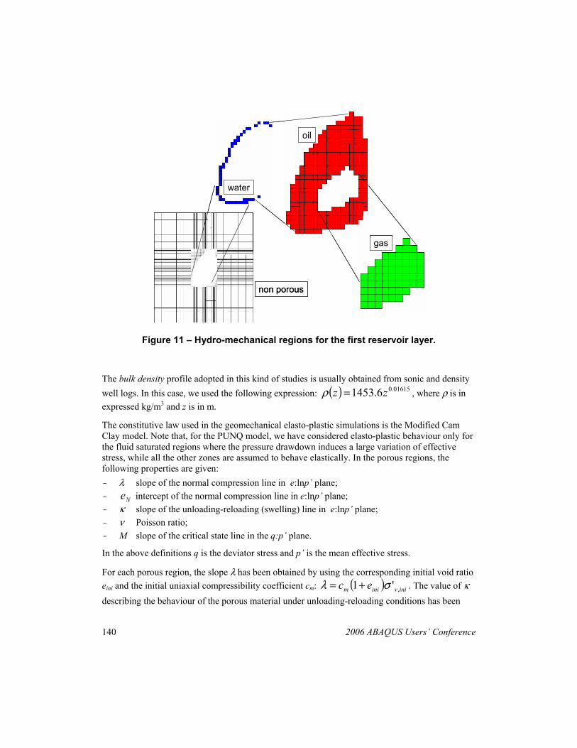
In Figure 11 we show the hydro-mechanical regions for the first reservoir layer: the green area is the gas saturated region (above the GOC, located at 2355 m), the red area is the oil saturated zone (below the GOC and above the WOC, located at 2395 m), the blue area is the water saturated region and the white area is the non-porous region.


gas

oil

water

non porous

gas

oil

water

non porous

Figure 11 – Hydro-mechanical regions for the first reservoir layer.

The bulk density profile adopted in this kind of studies is usually obtained from sonic and density well logs. In this case, we used the following expression: ( ) 01615.06.1453 zz =ρ , where ρ is in expressed kg/m3 and z is in m.

The constitutive law used in the geomechanical elasto-plastic simulations is the Modified Cam Clay model. Note that, for the PUNQ model, we have considered elasto-plastic behaviour only for the fluid saturated regions where the pressure drawdown induces a large variation of effective stress, while all the other zones are assumed to behave elastically. In the porous regions, the following properties are given: - λ slope of the normal compression line in e:lnp’ plane; - Ne intercept of the normal compression line in e:lnp’ plane; - κ slope of the unloading-reloading (swelling) line in e:lnp’ plane; - ν Poisson ratio; - M slope of the critical state line in the q:p’ plane.

In the above definitions q is the deviator stress and p’ is the mean effective stress.

For each porous region, the slope λ has been obtained by using the corresponding initial void ratio eini and the initial uniaxial compressibility coefficient cm: ( ) inivinim ec ,'1 σλ += . The value of κ describing the behaviour of the porous material under unloading-reloading conditions has been


assumed as 1/3 of the corresponding λ. The Poisson ratio is 0.3 and, finally, the slope M of the critical state line has been taken as 1.33.

The mechanical behaviour of the non-porous regions of the model is described by a linear isotropic elastic constitutive law by giving, as input to ABAQUS, the elasticity modulus E and the Poisson’s ratio ν.

The uniaxial compressibility cm, as a function of the effective stress, has been assumed to be:

)1347.1('01367.0 −= vmc σ

where σ’v is the vertical effective stress in bar. The vertical effective stress has been evaluated as pvv −= σσ ' , being σv the total vertical stress, calculated using the bulk density given above,

and p the pore pressure. In the overburden and underburden layers, p has been obtained through the following relationship (z in m and p in bar): p=0.102 z; while, for each region of the reservoir an average weighted on pore volume has been adopted.

After the initialization of the model, the pressure evolution has been imposed as a boundary condition at each node of the FE grid using 17 loading steps, approximately one per year of production of the field.

The FE model predicts a maximum forecasted subsidence of 0.81 cm, at the end of the production, compared to 0.65 cm given by the semi-analytical approximation. The maximum extent of the predicted iso-subsidence 0.05 cm line is around 6 km for the semi-analytical and 4.5 km for the elasto-plastic FE model. From Figure 12, it can be seen that the subsidence bowl presents the same nearly circular shape in all cases, and that it is much smaller for the elasto-plastic model than for the semi-analytical one: the subsidence bowl deepens in the case of elasto-plastic FE modelling but its effects are restricted to a smaller area.

The whole time evolution of the 0.05 cm iso-subsidence contour line is shown in Figure 13. It has to be noted, however, that the results in terms of subsidence are absolutely negligible since no measuring instrument has accuracy comparable to the results of our simulations (0.81 cm in 16 years). In fact, the iso-subsidence line of 2 cm is usually assumed to be the limit of subsidence.

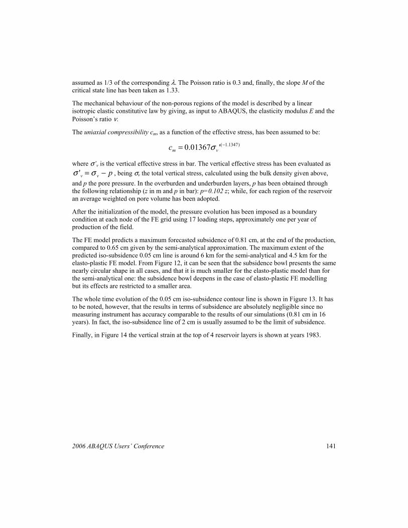
Finally, in Figure 14 the vertical strain at the top of 4 reservoir layers is shown at years 1983.


-6000 -4000 -2000 0 2000 4000 6000 8000 10000-5000

-4000

-3000

-2000

-1000

0

1000

2000

3000

4000

5000

6000

7000

8000

9000

10000

-6000 -4000 -2000 0 2000 4000 6000 8000 10000-5000

-4000

-3000

-2000

-1000

0

1000

2000

3000

4000

5000

6000

7000

8000

9000

10000

Figure 12 – Subsidence results: analytical (red), semi-analytical (blue), Elasto-plastic FE (black).

-6000 -4000 -2000 0 2000 4000 6000 8000 10000-5000

-4000

-3000

-2000

-1000

0

1000

2000

3000

4000

5000

6000

7000

8000

9000

10000

1970

19751983

-6000 -4000 -2000 0 2000 4000 6000 8000 10000-5000

-4000

-3000

-2000

-1000

0

1000

2000

3000

4000

5000

6000

7000

8000

9000

10000

1970

19751983

Figure 13 – Time evolution of 0.05-cm iso-subsidence contour line.


Top of layer 1

Top of layer 2

Top of layer 3

Top of layer 4

Figure 14 – Vertical strain maps at the top of 4 reservoir layers at year 1983.

6. Conclusions

The workflow presented in this paper has been applied in Eni E&P to real cases with excellent results in terms of compaction and subsidence evaluation associated with hydrocarbon production.


An open issue is related to the hydro-mechanical coupling between the flow and geomechanical solvers. Our plan for future work includes an iterative coupling between Eclipse and ABAQUS that will take into account the influence of porosity and permeability variations as computed by ABAQUS into Eclipse flow simulations.

7. References

1. Boot, R., “Level Control Surveys in the Groningen Gas Field”, Verhandelingen Kon. Ned. Geol. Mijnbouwk. Gen., Vol. 28, pp. 105-109, 1973.

2. Bruno, M. S., “Subsidence-Induced Well Failure”, SPE Drilling Engineering, 1992. 3. da Silva, F. W., Debande G. F., Pereira C. A., and Plischke B., “Casing Collapse Analysis

Associated With Reservoir Compaction and Overburden Subsidence”, SPE 20953, 1990. 4. Floris, F.J., Bush, M.D., Cuypers, M., Roggero, F., and Syversveen, A.R., “Comparison of

Production Forecast Uncertainty Quantification Methods - An Integrated Study”, paper presented at 1st Conference on Petroleum Geostatistics, Toulouse 1999.

5. Geertsma, J., “A Basic Theory of Subsidence due to Reservoir Compaction: the Homogeneous Case”, Verhandelingen Kon. Ned. Geol. Mijnbouwk. Gen., Vol. 28, pp. 43-62, 1973.

6. Geertsma J. and Van Opstal G., “A Numerical Technique for Predicting Subsidence Above Compacting Reservoirs Based on the Nucleus of Strain Concept”, Verhandelingen Kon. Ned. Geol. Mijnbouwk. Gen., Vol. 28, pp. 63-78, 1973a.

7. Mindlin R.D. and Cheng D.H., “Thermoelastic Stress in the Semi-Infinite Solid”, J. of Applied Physics, Vol. 21, p. 931-933, 1950.

8. Ostermeier, R. M., “Deepwater Gulf of Mexico Turbidites – Compaction effects on Porosity and Permeability”, SPE 26468, 1995.

9. Schlumberger, “Eclipse Reference Manual 2005A”, 2005. 10. The PUNQ Project, URL http://www.nitg.tno.nl/punq/. 11. Terzaghi, K., “The Shearing Resistance of Saturated Soils and the Angle Between the Plane

of Shear”, Proc. of 1st Int. SMFE Conference, Harvard Mass., Vol.1, pp. 54-56, 1936. 12. Zaman, M. M., Abdulrahheem, A. and Roegiers, J. C., “Reservoir Compaction and Surface

Subsidence in the North Sea Ekofisk field”, Subsidence due to fluid withdrawal, Elsevier Scince, pp. 373-419, 1995.

8. Acknowledgement

The authors acknowledge Eni S.p.A. for the permission to publish this paper. We are also grateful to R. Vitali and to E. Sguanci of ABAQUS Italia s.r.l. for their help.

numerical simulation of compaction and subsidence · pdf file2006 abaqus users’...

Documents