numerical optimization - linear programming -...

Numerical OptimizationLinear Programming - Duality

Shirish Shevade

Computer Science and AutomationIndian Institute of ScienceBangalore 560 012, India.

NPTEL Course on Numerical Optimization

Shirish Shevade Numerical Optimization

The Diet Problem: Find the most economical diet that satisfiesminimum nutritional requirements.

Number of food items: nNumber of nutritional ingredient: mEach person must consume at least bj units of nutrient j perdayUnit cost of food item i: ci

Each unit of food item i contains aji units of the nutrient jNumber of units of food item i consumed: xi

Constraint corresponding to the nutrient j:

aj1x1 + aj2x2 + . . . + ajnxn ≥ bj, xi ≥ 0 ∀ i

Cost:c1x1 + c2x2 + . . . + cnxn


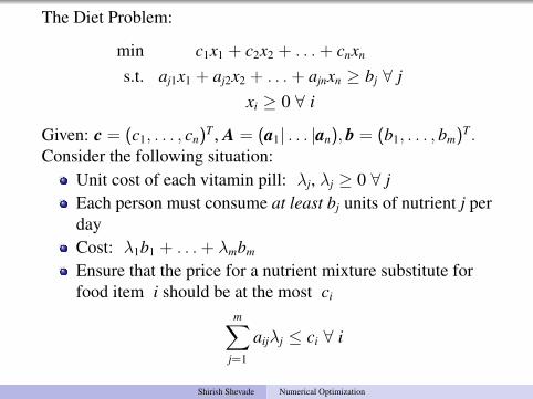
The Diet Problem:

min c1x1 + c2x2 + . . . + cnxn

s.t. aj1x1 + aj2x2 + . . . + ajnxn ≥ bj ∀ jxi ≥ 0 ∀ i

Given: c = (c1, . . . , cn)T , A = (a1| . . . |an), b = (b1, . . . , bm)T .

Consider the following situation:Unit cost of each vitamin pill: λj, λj ≥ 0 ∀ jEach person must consume at least bj units of nutrient j perdayCost: λ1b1 + . . . + λmbm

Ensure that the price for a nutrient mixture substitute forfood item i should be at the most ci

m∑j=1

aijλj ≤ ci ∀ i


The problem,

max λ1b1 + λ2b2 + . . . + λnbn

s.t. ai1λ1 + ai2λ2 + . . . + aimλm ≤ ci ∀ iλj ≥ 0 ∀ j

is the dual problem of

min c1x1 + c2x2 + . . . + cnxn

s.t. aj1x1 + aj2x2 + . . . + ajnxn ≥ bj ∀ jxi ≥ 0 ∀ i


Duality in Linear Programming

Symmetric Form of Duality

Primal Problem

min cTxs.t. Ax ≥ b

x ≥ 0

Dual Problem

max bTλ

s.t. ATλ ≤ cλ ≥ 0

Asymmetric form of Duality

Primal Problem

min cTxs.t. Ax = b

x ≥ 0

Dual Problem

max bTµ

s.t. ATµ ≤ c


Primal Problem


x ≥ 0

Dual Problem

max bTλ

s.t. ATλ ≤ cλ ≥ 0

For linear programs, the dual of the dual is the primal problem.

Primal Problem

−min −bTλ

s.t. −ATλ ≥ −cλ ≥ 0

Dual Problem


x ≥ 0


Consider the following primal and dual problems:

Primal Problem (P)

min cTxs.t. Ax = b

x ≥ 0

Dual Problem (D)

max bTµ

s.t. ATµ ≤ c

Weak Duality TheoremIf x and µ are primal and dual feasible respectively, thencTx ≥ bTµ.

Strong Duality TheoremIf either of the problems P or D has a finite optimal solution, sodoes the other, and the corresponding optimal objectivefunction values are equal. If any of these two problems isunbounded, the other problem has no feasible solution.


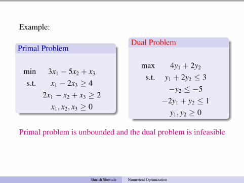
Example:

Primal Problem

min 3x1 − 5x2 + x3

s.t. x1 − 2x3 ≥ 42x1 − x2 + x3 ≥ 2

x1, x2, x3 ≥ 0

Dual Problem

max 4y1 + 2y2

s.t. y1 + 2y2 ≤ 3−y2 ≤ −5

−2y1 + y2 ≤ 1y1, y2 ≥ 0

Primal problem is unbounded and the dual problem is infeasible


Example:

Primal Problem

max x1 + x2

s.t. x1 − x2 ≤ 1−x1 + x2 ≤ −2

x1, x2 ≥ 0

Dual Problem

min y1 − 2y2

s.t. y1 − y2 ≥ 1−y1 + y2 ≥ 1

y1, y2 ≥ 0

Both primal and dual problems are infeasible


Example:

min 2x1 + 15x2 + 5x3 + 6x4

s.t. x1 + 6x2 + 3x3 + x4 ≥ 2−2x1 + 5x2 − x3 + 3x4 ≤ −3

x1, x2, x3, x4 ≥ 0

The dual problem is

max 2y1 − 3y2

s.t. y1 − 2y2 ≤ 26y1 + 5y2 ≤ 153y1 − y2 ≤ 5y1 + 3y2 ≤ 6

y1 ≥ 0, y2 ≤ 0


Solution of the primal problem using Simplex Method:

min 2x1 + 15x2 + 5x3 + 6x4

s.t. x1 + 6x2 + 3x3 + x4 ≥ 2−2x1 + 5x2 − x3 + 3x4 ≤ −3

x1, x2, x3, x4 ≥ 0

The equivalent problem is:

min 2x1 + 15x2 + 5x3 + 6x4

s.t. x1 + 6x2 + 3x3 + x4 ≥ 22x1 − 5x2 + x3 − 3x4 ≥ 3

x1, x2, x3, x4 ≥ 0

Phase I: Introducing artificial variables, the constraints become

x1 + 6x2 + 3x3 + x4 − x5 + x6 = 22x1 − 5x2 + x3 − 3x4 − x7 + x8 = 3

xj ≥ 0, j = 1, . . . , 8Shirish Shevade Numerical Optimization

Therefore, the artificial linear program is,

min x6 + x8

s.t. x1 + 6x2 + 3x3 + x4 − x5 + x6 = 22x1 − 5x2 + x3 − 3x4 − x7 + x8 = 3

xj ≥ 0, j = 1, . . . , 8

Initial Tableau:x1 x2 x3 x4 x5 x6 x7 x8 RHS1 6 3 1 -1 1 0 0 22 -5 1 -3 0 0 -1 1 30 0 0 0 0 1 0 1 0

Making the relative costs of basic variables 0,

x1 x2 x3 x4 x5 x6 x7 x8 RHS1 6 3 1 -1 1 0 0 22 -5 1 -3 0 0 -1 1 3-3 -1 -4 2 1 0 1 0 -5


Using Simplex Method, final tableau for the artificial linearprogram:

x1 x2 x3 x4 x5 x6 x7 x8 RHS0 17

5 1 1 −25

25

15 0 1

51 −21

5 0 -2 15 −1

5 −35 0 7

50 0 0 0 0 1 0 0 0

Basic variables for the original program: x1 = 7

5 , x3 = 15

Initial Tableau (for the original program):x1 x2 x3 x4 x5 x7 RHS0 17

5 1 1 −25

15

15

1 −215 0 -2 1

5 −35

75

2 15 5 6 0 0 0


Making the relatives costs of basic variables 0,x1 x2 x3 x4 x5 x7 RHS0 17

5 1 1 −25

15

15

1 −215 0 -2 1

5 −35

75

0 325 0 5 8

515 -19

5

Primal Problem

min 2x1 + 15x2 + 5x3 + 6x4

s.t. x1 + 6x2 + 3x3 + x4 ≥ 2−2x1 + 5x2 − x3 + 3x4 ≤ −3

x1, x2, x3, x4 ≥ 0

Dual Problem

max 2y1 − 3y2

s.t. y1 − 2y2 ≤ 26y1 + 5y2 ≤ 153y1 − y2 ≤ 5y1 + 3y2 ≤ 6

y1 ≥ 0, y2 ≤ 0

Optimal objective function = 195 (for both the problems)


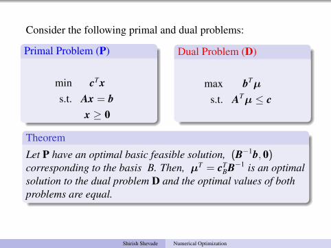
Consider the following primal and dual problems:

Primal Problem (P)

min cTxs.t. Ax = b

x ≥ 0

Dual Problem (D)

max bTµ

s.t. ATµ ≤ c

Theorem

Let P have an optimal basic feasible solution, (B−1b, 0)corresponding to the basis B. Then, µT = cT

BB−1 is an optimalsolution to the dual problem D and the optimal values of bothproblems are equal.


Proof.

x = (B−1b, 0) is an optimal basic feasible solution. Atoptimality, KKT conditions are satisfied. Therefore,

λTB = 0T , λT

N = cTN − cT

BB−1N ≥ 0T ⇒ cTBB−1N ≤ cT

N

Define, µT = cTBB−1.

∴ µTA = µT(B, N) = (cTB, cT

BB−1N) ≤ (cTB, cT

N) = cT

Therefore, µ is dual feasible.By Weak Duality Theorem, µTAx ≤ cTx ⇒ µTb ≤ cTx.Further, µTb = cT

BB−1b = cTBxB = cTx.

Thus, optimal values of P and D are equal.

How to obtain optimal µ after solving the primal problem?


LP in Standard Form:

min cTxs.t. Ax = b

x ≥ 0

where A ∈ Rm×n and rank(A) = m.Basic Nonbasic Artificial RHS

Variables Variables VariablesB N I bcT

B cTN 0T 0

(

I B−1N B−1 B−1bcT

B cTN 0T 0

)(

I B−1N B−1 B−1b0T cT

N − cTBB−1N −cT

BB−1 −cTBB−1b

)Shirish Shevade Numerical Optimization

LP in Standard Form:

min cTxs.t. Ax = b

x ≥ 0

where A ∈ Rm×n and rank(A) = m.(I B−1N B−1 B−1b

0T cTN − cT

BB−1N −cTBB−1 −cT

BB−1b

)At optimality of primal problem:

λTN = cT

N − cTBB−1N ≥ 0T

µT = cTBB−1 is an optimal solution to the dual problem


Consider the problem,min −3x1 − x2

s.t. x1 + x2 ≤ 2x1 ≤ 1

x1, x2 ≥ 0

and its dual problem:

max 2λ1 + λ2

s.t. λ1 + λ2 ≤ −3λ1 ≤ −1λ1, λ2 ≤ 0

Optimal primal objective function = −4 at x∗ = (1, 1)T

Optimal dual objective function = −4 at λ∗ = (−1,−2)T


min −3x1 − x2

s.t. x1 + x2 + x3 = 2x1 + x4 = 1

x1, x2, x3, x4 ≥ 0

Initial Basic Feasible Solution:xB = (x3, x4)

T = (2, 1)T , xN = (x1, x2)T = (0, 0)T

Initial Tableau: x1 x2 x3 x4 RHS1 1 1 0 21 0 0 1 1-3 -1 0 0 0


Initial Tableau: x1 x2 x3 x4 RHS1 1 1 0 21 0 0 1 1-3 -1 0 0 0

Final Tableau:

x1 x2 x3 x4 RHS0 1 1 -1 11 0 0 1 10 0 1 2 4

Optimal primal solution: x∗ = (1, 1)T

Optimal dual solution: λ∗ = (−1,−2)T


numerical optimization - linear programming -...

Documents