Environ Fluid MechDOI 10.1007/s10652-011-9209-0

ORIGINAL ARTICLE

Numerical modeling of aquaculture dissolved wastetransport in a coastal embayment

Subhas K. Venayagamoorthy · Hyeyun Ku ·Oliver B. Fringer · Alice Chiu · Rosamond L. Naylor ·Jeffrey R. Koseff

Received: 2 November 2009 / Accepted: 20 January 2011© Springer Science+Business Media B.V. 2011

Abstract Marine aquaculture is expanding rapidly without reliable quantification of efflu-ents. The present study focuses on understanding the transport of dissolved wastes fromaquaculture pens in near-coastal environments using the hydrodynamics code SUNTANS(Stanford Unstructured Nonhydrostatic Terrain-following Adaptive Navier–Stokes Simula-tor), which employs unstructured grids to compute flows in the coastal ocean at very highresolution. Simulations of a pollutant concentration field (in time and space) as a function ofthe local environment (bathymetry), flow conditions (tides and wind-induced currents), andthe location of the pens were performed to study their effects on the evolution of the waste

S. K. Venayagamoorthy (B) · H. KuDepartment of Civil and Environmental Engineering, Colorado State University, Fort Collins,CO 80523-1372, USAe-mail: vskaran@colostate.edu

H. Kue-mail: hyeyun@engr.colostate.edu

O. B. Fringer · J. R. KoseffEnvironmental Fluid Mechanics Laboratory, Department of Civil and Environmental Engineering,Stanford University, Stanford, CA 94305, USA

O. B. Fringere-mail: fringer@stanford.edu

J. R. Koseffe-mail: koseff@stanford.edu

A. Chiu · R. L. NaylorProgram on Food Security and the Environment, Stanford University, Stanford, CA 94305, USA

A. Chiue-mail: alchiu@stanford.edu

R. L. Naylore-mail: roz@stanford.edu

O. B. Fringer · R. L. Naylor · J. R. KoseffWoods Institute for the Environment, Stanford University, Stanford, CA 94305-4205, USA

123

Environ Fluid Mech

plume. The presence of the fish farm pens cause partial blockage of the flow, leading to thedeceleration of the approaching flow and formation of downstream wakes. Results of boththe near-field area (area within 10 to 20 pen diameters of the fish-pen site) as well as far-fieldbehavior of the pollutant field are presented. These detailed results highlight for the first timethe importance of the wake vortex dynamics on the evolution of the near-field plume as wellas the rotation of the earth on the far-field plume. The results provide an understanding ofthe impact of aquaculture fish-pens on coastal water quality.

Keywords Effluent pollution · Dispersion · Aquaculture · Numerical modeling ·Plume dynamics · Coastal engineering

1 Introduction

The rapid expansion of marine aquaculture is a potential solution to the problem of overfish-ing and fisheries depletion worldwide, but also a major threat to ocean ecosystems. One ofthe most widely cited but poorly quantified impacts of open netpen aquaculture is its releaseof nutrients and other wastes to the surrounding environment [14]. In the United States thereis considerable pressure on state and federal agencies to regulate the growth and mitigatethe impacts of aquaculture operations in coastal waters [13]. In May 2006, the Californialegislature passed the California Sustainable Oceans Act (SOA) to establish regulations thatensure marine finfish aquaculture operations in state waters are environmentally sustainable(see Box 1). The framework for evaluating environmental impacts and proper siting of aqua-culture facilities is expected to be certified by the Department of Fish and Game by thefall of 2011. However, there remains much uncertainty regarding the environmental impactsof aquaculture operations and the appropriate (and reliable) methods for regulating theseimpacts. The goal of this study is to adapt and employ a highly-resolved numerical model-ing tool that will allow the user to predict the impact of a particular aquaculture operationon water quality in a coastal environment. In particular, we seek to answer the questions:Where and in what concentrations will the dissolved waste from aquaculture pens locatedin near-shore and off-shore environments be found, and what will the impact be on waterquality?

Proper assessment of the potential impact of a fish farm with several pens is closely linkedto the mixing and dispersal of the waste discharge from the pens with the ambient flow [9].The dispersal of wastes from pens released into the coastal ocean may not be necessarily“Gaussian” (monotonically decreasing from the source in all directions) and therefore ‘dilu-tion may not be the solution’ contrary to what is often claimed. The evidence from previouslaboratory and field studies [5,19] suggests that wastes may be transported in plumes thatretain their coherence and maintain relatively high concentrations over large distances. Thispattern of dispersal could result in much higher concentrations of wastes at certain points onthe coastline, even at considerable distances from the source.

There is very little work in the refereed literature describing the dispersal of aquaculturewastes under varying hydrodynamic conditions at the field scale. Previous numerical studieshave focused mostly on the near-field mixing under steady uni-directional flow conditions[9]. Some recent field measurements on mussel and shellfish aquaculture identify the envi-ronmental impacts of large farms which include wave attenuation and flow suppression dueto interaction with stratification [6,15,20]. The complex nature of the flow around fish pensis caused by flow separation due to partial blockage of the flow by the pens and the combined

123

Environ Fluid Mech

effects of tides and winds. At larger scales, the influence of the earth’s rotation becomesimportant and can alter the evolution of the waste plume considerably.

Using representative field-scale physical and flow parameter values in our model, weare able to address a number of policy-relevant issues. For example, the model can assistwith siting decisions by taking into account local currents and flow conditions to identifylocations where dissolved wastes could negatively impact other users, public trust values,or the marine environment (factor 1 in Box 1). Knowing the spatial distribution of effluentsemitted from a net pen allows one to better understand the effects of that pen on sensitivehabitats, ecosystems, other uses, and plant and animal species, including marine mammalsand birds, in the vicinity (factors 2, 3, 4, 6 in Box 1). The modeling technique can be mostdirectly applied to factor number 5 in determining the extent and concentration of a varietyof products, pollutants, and nutrient wastes over space and time. Future development of themodel may also lend insight to the interactions among effluents from several farms sitedtogether (i.e., cumulative effects as mentioned in factor 7). While certainly not a substitutefor on-the-ground monitoring, the effluent model can be a useful tool for predicting a site’sability to meet water quality standards before aquaculture operations are established. Themodel allows a potential aquaculture operator to provide a more accurate description ofthe expected discharge(s) from their facility in the Notice of Intent submitted to the waterboards [3].

Box 1: PEIR requirements as set out in the California Sustainable Oceans Act(SOA). The first step in implementing the SOA is the preparation of a programmaticenvironmental impact report (PEIR), which is currently being drafted. The Actdescribes the purpose of the PEIR: …the report shall provide a framework for man-aging marine finfish aquaculture in an environmentally sustainable manner that, ata minimum, adequately considers all of the following factors:

1. Appropriate areas for siting marine finfish aquaculture operations to avoidadverse impacts, and minimize any unavoidable impacts, on user groups, publictrust values, and the marine environment.

2. The effects on sensitive ocean and coastal habitats.3. The effects on marine ecosystems, commercial and recreational fishing, and other

important ocean uses.4. The effects on other plant and animal species, especially species protected or

recovering under state and federal law.5. The effects of the use of chemical and biological products and pollutants and

nutrient wastes on human health and the marine environment.6. The effects of interactions with marine mammals and birds.7. The cumulative effects of a number of similar finfish aquaculture projects on the

ability of the marine environment to support ecologically significant flora andfauna.

8. The effects of feed, fish meal, and fish oil on marine ecosystems.9. The effects of escaped fish on wild fish stocks and the marine environment.

10. The design of facilities and farming practices so as to avoid adverse environmen-tal impacts, and to minimize any unavoidable impacts.(California F&GC Code [2]).

123

Environ Fluid Mech

While policy applications are the end goal, our initial focus, and the focus of this paper,is simpler. We are modeling the dispersal of “dissolved wastes” (considered here as passivescalars) such as nitrogen and phosphorus from aquaculture pens using high-resolution, two-dimensional, depth-averaged numerical simulations under different time-varying flows in anidealized coastal embayment. We highlight the different dispersal patterns that may occurunder various forcing scenarios (flows, tides, earth’s rotation, and local sources) in a moreidealized model bathymetry. The layout of this paper is as follows: In Sect. 2, we brieflydescribe the computational approach we employ for this study, provide an overview of theproblem set-up and outline a summary of all the simulation cases that will be discussed inSect. 3. We then present and discuss results of the lateral mixing of a continuous pollutantsource emanating from single pen in a channel flow as well as from an array of aquaculturepens in a idealized coastal embayment under different flow conditions in Sect. 3. Finally wedraw some conclusions and provide some directions for future work in Sect. 4.

2 Numerical methodology and problem configuration

2.1 Numerical methodology

We employ the SUNTANS code developed by Fringer et al. [8] to perform highly resolvedsimulations of flow through and around fish pens in the idealized coastal embayment shownin Fig. 1. SUNTANS is an unstructured, finite-volume, parallel coastal-ocean simulator thatsolves the three-dimensional nonhydrostatic Navier–Stokes equations with the Boussinesqapproximation in a rotating frame. It also solves for the free surface as well as the transportof salinity and temperature (see Fringer et al. [8] and Wang et al. [21] for details). This codehas been applied to a host of coastal problems and processes such as the generation andevolution of internal waves in Monterey Bay [11] and the South China Sea [22] and high-resolution simulations of estuarine hydrodynamics [21]. However, in this study, we use thedepth-averaged formulation of SUNTANS using a single vertical layer for all the simulations.Hence, the governing equations revert to the two-dimensional shallow water equations (alsoknown as the Saint-Venant equations), together with the depth-averaged continuity equationgiven by

∂u

∂t+ u

∂u

∂x+ v

∂u

∂y− f v = −g

∂h

∂x+ νH

(∂2u

∂x2 + ∂2u

∂y2

)

+ τ sx

H− CDB

√u2 + v2

Hu + FD,x, (1)

∂v

∂t+ u

∂v

∂x+ v

∂v

∂y+ f u = −g

∂h

∂y+ νH

(∂2v

∂x2 + ∂2v

∂y2

)

+ τ sy

H− CDB

√u2 + v2

Hv + FD,y, (2)

∂h

∂t+ ∂

∂x(Hu) + ∂

∂y(Hv) = 0, (3)

where H = h + d is the total water depth in m, h is the free-surface height relative to somevertical datum in m, d is the depth of the bottom relative to some vertical datum in m, u, v

are the horizontal cartesian components of the depth-averaged velocity vector in m s−1, t istime in s, g is the constant of gravitational acceleration in m s−1, f = 2�earth sin φlat is

123

Environ Fluid Mech

the Coriolis parameter with �earth been the angular velocity of the earth’s rotation in s−1 andφlat the latitude, νh is the horizontal eddy viscosity in m2 s−1, τ s

x and τ sy are the free-surface

stresses at z = h,CDB is a non-dimensional bottom drag coefficient and FD,x and FD,y

are the pen-induced drag forces in the x and y directions respectively, and are given by aquadratic drag law formulation as shown in (5).

We opted to use the two-dimensional depth-averaged formulation since this study is a firststep in addressing far-field influence of the near-field dynamics, with a particular emphasison the near-field vortex street which is predominantly two-dimensional. Furthermore, thetwo-dimensional highly resolved simulations on their own are computationally intensive andtherefore three-dimensional simulations and associated parameter studies were not feasibledue to computational and time constraints for the scope of work we have performed usingthe two-dimensional simulations.

2.2 Problem configuration

The domain we use for the main part of this study is a model coastal embayment that is 10km in length and 5 km wide as shown in Fig. 1. The bathymetry of the domain consists ofa shallow embayment incised by a deep channel as shown in Fig. 2. Two sets of 6 20 mdiameter fish pens are used in this study, as shown in Fig. 1, and the fish pens are all locatedclose to the western edge of the embayment. We present results showing the effect of varyingthe location of the pens on the dispersal of the waste plume in Sect. 3.

At the alongshore boundaries of the domain shown in Fig. 1, we impose a velocity fieldof the form

Fig. 1 Unstructured computational mesh showing the embayment used in the simulations for this study. Avelocity field described by Eq. 4 is imposed at the northern boundary of the domain with a M2 tidal frequencyof 1.4 × 10−4 rad s−1. The image on the right shows a zoomed view highlighting the grid refinement aroundan array of six 20 m diameter pens

123

Environ Fluid Mech

Fig. 2 Idealized depth contours of the model embayment depicting a shallow shelf incised by a deep channel.Locations of model fish pens are depicted by the white boxes (for the offshore cases listed in Table 1). Thedepth is indicated by the color bar in meters

v = Um + UT sin(ωt), (4)

where Um ≤ 0 is the amplitude of the mean current (where flow is in the north-south direc-tion); UT is the amplitude of the sinusoidal tidal component of the flow field with forcingfrequency ω; and v is the alongshore component of the velocity field. Boundary conditionsfor the horizontal velocity v are free-slip along the coastline and offshore boundary. Thehorizontal component in the x-direction of the velocity field u has no-flux boundary condi-tions along the coastline and the offshore boundary. The scalar field has no-flux boundaryconditions on all boundaries. An unstructured mesh is generated for this study with a total ofapproximately 162,500 cells, with grid refinement in the vicinity of the fish pens as shownin Fig. 1. The resolution near the pens is roughly 5 m, while that in the far-field is stretchedto 50 m. Each individual fish pen is cylindrical in shape with a diameter of D = 20 m. Adrag law formulation is employed to account for the flow reduction inside the pens and theresulting decrease in momentum downstream of the pens. This drag formulation is given bya quadratic drag-law on the right-hand side of the x- and y-momentum equations shown in(1) and (2) and are of the form

123

Environ Fluid Mech

FD,x = −αCD(u2 + v2)1/2

Du,

FD,y = −αCD(u2 + v2)1/2

Dv, (5)

where CD is the non-dimensional drag coefficient exerted by the fish pens, u and v are theCartesian components of the velocity vector, and α = 1 inside of the pens while α = 0outside of the pens. We use a horizontal eddy-viscosity of νh = 10−3 m2 s−1, and a qua-dratic bottom drag law formulation (as shown in (1) and (2)) with a drag coefficient ofCD,bottom = 0.0025. An estimate of the Reynolds number based on a characteristic veloc-ity scale of 0.1 m s−1 and the specified values of D = 20 m and νh = 10−3m2 s−1 isRe = 2000. A continuous pollutant (scalar) point source is placed inside the perimeter ofeach pen as an approximation of the effluent waste discharged from the pens. No horizontalscalar diffusivity is employed since it is assumed that transport dominates the dispersion.Transport is computed with a high-resolution total variation diminishing (TVD) scheme, asimplemented by Zhang and Fringer [22]. The TVD scheme is explicit and hence conditionallystable but it guarantees monotonicity. For all simulations, we restrict the time step such thatthe maximum Courant number, based on the smallest grid spacing and the maximum currents,is roughly 0.5. This provides sufficient temporal resolution while maintaining stability.

An important non-dimensional parameter for the simple model flow problem defined by(4) is the ratio of the tidal to mean flow given by

η = UT

Um

, (6)

which compares the amplitude of the oscillatory flow to the amplitude of the mean currentand is an important parameter that determines the shape of the contaminant plume [16]. Asecond important parameter is the non-dimensional tidal excursion lengthscale given by

K = 2UT

ωD, (7)

where UT is the amplitude of the tidal current, ω is the forcing frequency and D is the pendiameter. This represents the ratio of the tidal excursion to the pen diameter and is analo-gous to the Keulegan-Carpenter number used in wave-structure interaction studies. For all ofthe simulations performed in this study, we have used an alongshore velocity magnitude ofUm = 0.1 m s−1, which is representative of mean currents in coastal regions such as the St.Lawrence Island in the Bering Sea. The tidal velocity magnitude is varied to yield different(field-scale) values of η and K . In Sect. 3, we discuss the influence of these and other param-eters on the dispersion of a contaminant plume in the idealized coastal embayment shown inFig. 1.

2.3 Simulation cases

We performed a total of 11 simulations for this study as shown in Table 1. The first foursimulations (cases 1 through 4) are used as test cases to show the transverse mixing of aplume around a cylindrical 20 m diameter pen in a rectangular open channel that is 3 kmlong and 1 km wide. Case 1 will be used to highlight the classical Gaussian behavior ofthe plume in a uni-directional flow in the absence of rotation and without pen-induced drag(CD = 0) and validate the numerical model results with analytical/empirical results of plumedynamics. Cases 2 and 3 are also uni-directional channel flow cases with pen-induced drag

123

Environ Fluid Mech

Table 1 Summary of the 11 cases simulated in the present paper. The last column provides some remarkswhere the Rossby number (Ro = Um/(f L), where L = 5 km) and other variables and/or comments areshown

Case # Case name Domain CD η K Remarks

1 Steady flow Channel 0 0 0 Ro = ∞2 Steady flow Channel 0.5 0 0 Ro = ∞3 Steady flow Channel 1.0 0 0 Ro = ∞4 Uniform + Oscillating flow Channel 1.0 1 46 Ro = ∞5 Offshore base case Embayment 1.0 1 71 Ro = 0.26

6 Offshore with no rotation Embayment 1.0 1 71 Ro = ∞7 Offshore with river inflow Embayment 1.0 1 71 UR/Um = 0.5

8 Offshore with no pen drag Embayment 0 1 71 Ro = 0.26

9 Nearshore base case Embayment 1.0 1 71 Ro = 0.26

10 Nearshore with strong tides Embayment 1.0 2 71 Ro = 0.26

11 Nearshore with wind Embayment 1.0 ∞ 71 u10 = 10 m s−1

coefficients CD = 0.5 and 1, respectively. These two cases will be used to demonstrate theeffects of the drag force induced by a pen on the lateral mixing of the plume and to provide ameasure of the model sensitivity on CD . Case 4 is presented to highlight the added effect oftidal oscillation (with η = 1,K = 46 and CD = 1) compared to case 3 (with η = 0,K = 0and CD = 1).

The remaining seven simulations are of the coastal embayment shown in Fig. 1 for differ-ent flow conditions and locations. Case 5, which we refer to as the ‘offshore base case’, takesinto account the drag induced by each of the 12 pens with CD = 1. We have also includedthe earth’s rotation with a Coriolis parameter of f = 8.7 × 10−5 rad s−1. The flow field isdriven by a tidal flow from north to south combined with a southerly flowing mean currentas described by (4). The relevant oscillating flow parameters are η = 1 and K = 71, basedon a tidal velocity amplitude of UT = 0.1 m s−1 and M2 tidal period of 12.42 h.

Case 6 shows a similar simulation to case 5 except that here, the Coriolis terms in themomentum equations ((1) and (2)) were switched off by simply setting f = 0. Case 7presents a simulation where we have added a river inflow to case 5, with all other parame-ters kept identical to case 5. A small river inflow river discharge with a velocity of UR =0.05 m s−1 was placed symmetrically at the channel incision at the central embayment coast(i.e. at a alongshore distance of 0 m). The width of the river inflow is 400 m and the dis-charge is approximately 1500 m3 s−1. This is about 10% of the volume flow rate entering theembayment from the northern alongshore boundary from the mean and tidally-induced flow.Case 8 is a simulation where the pen-induced drag is switched off (CD = 0) with all otherparameter kept identical to the ’offshore base case’ (case 5).

Case 9 is what we refer to as the ‘nearshore base case’ in Table 1. Our goal here is toexplore the variability in the plume dispersion as a function of the location of the pens. Awhole range of scenarios are possible and would be prohibitively expensive to completelysimulate computationally. Here, the southern facing farm in Fig. 1 was moved into the bayand closer to the channel incision (see Fig. 15). All other conditions remain unchanged rela-tive to the ‘offshore base case’. Case 10 is also a nearshore simulation (where the pens are inthe same locations as case 9) with a stronger tidal signal (η = 2) compared to the ‘nearshorebase case’ where η = 1. As discussed earlier in Sect. 2.2, η influences the shape of the

123

Environ Fluid Mech

plume. When η > 1, plume reversals will occur and dramatic changes to the plume structurecan be expected. Case 11 presents a nearshore simulation where surface wind stress acts overthe entire embayment in a northerly direction (i.e. opposite to the tidal flow). We have alsoremoved the mean current for this case in order to explore the effect of the wind-inducedcirculation on the plume distribution.

It is important to note that the point of these simulations is not to perform a parameterstudy to investigate the quantitative effects of a single parameter on the dispersion, but ratherto demonstrate the pronounced variability of the contaminant plume and how it is highlysensitive to different environmental forcing scenarios.

2.4 Statistical parameters for assessing plume distribution

Statistical indicators such as moments of non-dimensional plume concentration can providequantitative information on the plume characteristics. We compute the moments of the along-shore concentration distributions i.e. the mean, standard deviation, skewness, and kurtosis forall the embayment cases (cases 5–11). Here, we provide a description of these key statisticalparameters that will be used for discussing the alongshore plume distribution in Sect. 3.

The standard deviation provides an indication of spread (or dispersion) of a distributionand is defined as the root-mean-square of the concentration values (also defined as the squareroot of the variance) from their mean and given by

σ = √m2 =

√∑Nj=1

(Cj − C

)2

N, (8)

where C is the mean of the concentration distribution, N is the sample size and m2 is thevariance or the second moment about the mean. The skewness provides an indication of thedegree of asymmetry of a distribution when compared to the perfectly symmetrical Gaussiandistribution and is defined as the third moment about the mean normalized by the cube of thestandard deviation (see Eq. 9), while the kurtosis provides a measure of peakedness of a dis-tribution usually taken relative to a Gaussian distribution (noting that a Gaussian distributionhas a kurtosis of 3) and is given by the fourth moment about the mean divided by the variance(see Eq. 10). A concentration distribution with large kurtosis indicates strong intermittencywhile a distribution with large skewness indicates a highly asymmetrical distribution.

γ = m3√m3

2

=1N

∑Nj=1

(Cj − C

)3

(1N

∑Nj=1

(Cj − C

)2)3/2 , (9)

β = m4

m22

=1N

∑Nj=1

(Cj − C

)4

(1N

∑Nj=1

(Cj − C

)2)2 . (10)

3 Results and discussion

In this section, we first present results from the channel flow test cases (cases 1 through 4)to show the lateral mixing of a plume around a cylindrical fish pen in a rectangular channel.The goal is to highlight the classical behavior of the plume and the enhanced mixing thatoccurs due to vortices introduced by flow separation around a fish pen. We then focus our

123

Environ Fluid Mech

Fig. 3 Time-averaged normalized concentration field (shown in color) for a steady uni-directional test flowcase (case 1 in Table 1). The dashed red line shows the classical spread of a Gaussian plume using a lateraldiffusivity of 0.03 m2 s−1

attention mainly on the discussion of the simulation results of the coastal embayment underdifferent flow conditions and pen locations (simulation cases 5 through 11).

3.1 Channel cases (cases 1 through 4)

We performed a series of two-dimensional, depth-averaged simulations in an idealized rect-angular channel for a wide parameter space in CD,K and η to investigate their effects ondispersion. Here we present results and discussion to provide validation for our numericalmodel with a well known empirical relationship for the transverse (lateral) mixing coeffi-cient, and to highlight the enhanced mixing caused by the pen-induced drag compared to theclassical dispersion (case 1).

The time-averaged non-dimensional concentration (hereafter concentration will be used toimply non-dimensional concentration) field for the steady uni-directional channel flow case(case 1) is shown in Fig. 3. The spanwise concentration distributions at sections (a–a), (b–b)and (c–c) are shown in Fig. 4, respectively. The dashed red line in Fig. 3 shows the classicalspread of the plume width using an empirical lateral mixing coefficient εt /(du∗) = 0.15,

where d is the water depth and u∗ is the shear velocity [7,12]. It should be noted that thenondimensional lateral mixing coefficient was in the range of 0.1–0.2 in the experiments andhence 0.15 is considered as an average value. It is well known from experiments [1,7,12]and direct numerical simulations of channel flows (see for example Hoyas and Jimenez [10])that the mean velocity U is approximately 25u∗. Using this relationship, gives a value forεt = 0.03 m2 s−1. This is in good agreement with the lateral diffusivity of 0.026 m2 s−1

computed from the variances of the concentration distributions shown in Fig. 4. It can beseen from Fig. 3 that the x1/2 growth for the plume width predicted by the Gaussian for-mulation agrees reasonably well with the simulated concentration distribution. Also, all theconcentration profiles at the cross sections shown in Fig. 4 show close agreement with theGaussian plume. However, there is some divergence from the purely Gaussian case. This isprobably a consequence of the averaging from the numerical simulations. It takes a lot ofensembles to get pure Gaussian plots in experiments and numerical simulations.

Figures 5 and 7 show the time-averaged concentration fields for cases 2 and 3 shownin Table 1, respectively. The pen-induced drag coefficient for case 2 is CD = 0.5 and forcase 3, CD = 1. It is evident that the plume spread is enhanced by the drag induced by thepen for both cases. Rummel et al. [17] also observed enhanced plume growth (similar to

123

Environ Fluid Mech

Fig. 4 Time-averaged concentration distributions (solid lines) at a x = 500 m, b x = 1000 m and c x =2000 m. The red dashed lines are the Gaussian profiles calculated using a transverse mixing coefficient of0.03 m2 s−1, for the steady uni-directional test flow case shown in Fig. 3

Fig. 5 Time-averaged normalized concentration field (shown in color) for case 2 shown in Table 1. Thedashed red line shows the classical spread of a Gaussian plume using a lateral diffusivity of 0.03 m2 s−1

Fig. 6 Time-averaged concentration distributions (solid lines) for case 2 shown in Fig. 5 at a x = 500 m, bx = 1000 m and c x = 2000 m. The dashed red lines are the Gaussian profiles calculated using a transversemixing coefficient of 0.03 m2 s−1 for case 1

Figs. 5, 7) in their shallow free-surface flow with grid turbulence experiments. The corre-sponding spanwise concentration distributions at sections (a–a), (b–b) and (c–c) are shownin Figs. 6 and 8, respectively. These profiles highlight how the plumes in cases 2 and 3 (underthe influence of pen-induced drag) begin to depart quite early (at x = 500 m) from the clas-

123

Environ Fluid Mech

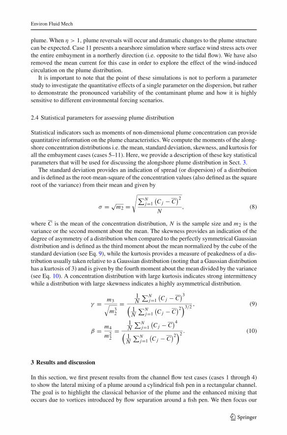
Fig. 7 Time-averaged normalized concentration field (shown in color) for case 3 shown in Table 1. Thedashed red line shows the classical spread of a Gaussian plume using a lateral diffusivity of 0.03 m2 s−1

Fig. 8 Time-averaged concentration distributions (solid lines) for case 3 shown in Fig. 7 at a x = 500 m, bx = 1000 m and c x = 2000 m. The dashed red lines are the Gaussian profiles calculated using a transversemixing coefficient of 0.03 m2 s−1 for case 1

sical Gaussian plume. The plumes spread nearly twice as wide compared to the classical case(case 1) at x = 2000 m as shown in Figs. 6c and 8c, respectively. The average lateral diffu-sivities computed from the variances of the time-averaged concentration fields at the differentcross sections are approximately 0.1 m2 s−1 for case 2 and 0.15 m2 s−1 for case 3, respec-tively. These values are about 3 to 5 times larger than the lateral mixing coefficient computedfor case 1. This clearly shows the dramatic effect of the pen-induced drag on the plumedynamics. A higher value of the drag coefficient CD results in a stronger vortex street thatappears to enhance the lateral mixing considerably. These results highlight the importanceof accounting for the presence of the pens in plume dispersion calculations.

Figure 9 shows the results of case 4. Here, the mixing and transport of a continuous pointsource scalar collocated within one fish pen is shown using a time sequence of the concentra-tion field over a duration of nearly two tidal periods (with T = 8 h, K = 46, η = 1, Um =0.1 m s−1) under oscillatory flow conditions. When the tidal component is in phase with themean current, the flow evolves in a similar manner to that of a uni-directional flow case (e.g.cases 2 and 3) with the usual formation of an unstable downstream wake resulting in vortexshedding (Fig. 9a, b). Soon after the initial vortex shedding begins, the flow starts to retardas the tidal velocity reverses direction and increases in amplitude. This causes the plume tocontract in the longitudinal direction with a simultaneous dispersion in the lateral direction asshown in Fig. 9c, d, and during the subsequent tidal cycle in Fig. 9g, h, respectively. Note how

123

Environ Fluid Mech

Fig. 9 Normalized concentration field (shown in color) for an oscillatory test flow case (UT /Um = 1, K = 46,

case 4 in Table 1). The continuous point source is located within the perimeter of the fish pen. Time is nor-malized by the tidal period T = 8 h

Fig. 10 Time-averaged normalized concentration field (shown in color) for an oscillatory test flow case (case4 in Table 1) with K = 46 and η = 1

the vortex shedding is also attenuated during this period. This behavior was first describedby Chatwin [4], where he points out that the contaminant cloud appears to be periodicallyexpanding and contracting. The plume is stretched during the period of high flow during

123

Environ Fluid Mech

the first half of the tidal cycle and contracts during the second half-cycle (see also [18])The time-averaged concentration field is shown in Fig. 10, which clearly demonstrates theenhanced dispersion that occurs under oscillatory flow conditions compared to the classicaldispersion (case 1) that would occur under uni-directional flow conditions. The slight asym-metry in the time-averaged concentration field in Fig. 10 is due to the finite number of tidalcycles over which the averaging is performed. This results in a distribution that is skewedin the direction of a set of counter-rotating vortices that emerge in the positive y-directionupon the first tidal reversal, as depicted in Figs. 9c, d. As shown in Figs. 9e, f, these counter-rotating vortices move in the positive y-direction, thereby causing a skew in the averagedconcentration field. Subsequent ejections of counter-rotating vortices are not as strong andtherefore, opposite-signed vortices do not counteract the effect of the first pair unless manymore tidal cycles are computed. We should also note that the asymmetry is accentuated bythe logarithmic concentration contours. Regardless, these results indicate that the mixing anddispersion of the pollutant field under oscillatory flow conditions with pen-induced drag isvery different (and enhanced) from a classical uni-directional flow case without pen-induceddrag (see Fig. 3). It is also worth noting that the plume growth in case 4 is further enhancedcompared to cases 2 and 3, which indicates that the combined action of pen-induced drag andoscillations in the flow field is very effective in mixing the plume laterally. As a comparison,the spread of the plume at x = 2000 m for case 4 is almost twice as wide as that of case 3at the same location.

3.2 Embayment results

Here, we present the results of all the embayment simulation cases presented in Sect. 2.3 andTable 1.

3.2.1 Offshore base case (case 5)

The passive scalar concentration field from a simulation run with two sets of fish farm penslocated along the edge of the embayment is shown in Fig. 11 as a time sequence over aduration of six tidal periods. For this ‘offshore base case’, we have included the drag inducedby each of the pens on the flow field and have also taken into account the earthc6s rotation.Using a Coriolis parameter of f = 8.7 × 10−5 rad s−1, and the embayment width as thelength scale, the Rossby number for this case is R = Um/f L = 0.26, which indicatesthat the Coriolis force will likely influence the flow dynamics. The flow field is driven bya tidal flow from north to south combined with a southerly flowing mean current. The rel-evant oscillating flow parameters as shown in Table 1 are η = 1 and K = 71, based ona tidal velocity amplitude of UT = 0.1 m s−1 and M2 tidal period of 12.42 h. The forma-tion of the downstream vortex shedding is evident early on as shown in Fig. 11a. As theflow reverses, the plume contracts in a similar manner to that observed for the channel flowtest case shown in Fig. 9. The plume, while predominantly transported downstream (south-wards) due to the rather strong mean current, also tends to spread eastward into the bay (seeFig. 11c–f).

Figure 12 shows the concentration distribution for all the offshore cases (cases 5–8)outlined in Table 1 at time t = 4T to highlight the differences in the plume behavior betweenthese cases. To assess the dispersion characteristics of the concentration plumes, we analyzedlongitudinal profiles of the concentration along the coastline as shown in Fig. 13 at times

123

Environ Fluid Mech

Fig. 11 “Birds-eye-view” of the time history of the normalized concentration in the vicinity if two sets of 620 m diameter pens (depicted as white boxes) releasing a passive scalar at the edge of the coastal embaymentfor the ‘offshore base case’ (case 5)

t = 3T and 6T , respectively. The alongshore concentrations profiles for cases 6, 7 and 8 arealso shown in Fig. 13 for comparison. These profiles for the ‘offshore base case’ clearly showthat the waste plume disperses toward the embayment coast albeit at very low concentrationlevels.

We computed the moments of the alongshore concentration distribution (as discussed inSect. 2.4 for all the embayment cases) and the statistics are shown in Tables 2 and 3. Alsoshown in Tables 2 and 3 are the peak values of the concentration for all the embayment casesoutlined in Table 1 at t = 3T and 6T , respectively. Time series of the concentration profilesat three locations along the embayment coastline highlight the temporal intermittency inthe concentrations along the embayment coast (see Fig. 14). Details of the results of thesesimulations are discussed in what follows.

123

Environ Fluid Mech

Fig. 12 “Birds-eye-view” of the time history of the normalized concentration in the vicinity if two sets of 620 m diameter pens (depicted as white boxes) releasing a passive scalar at the edge of the coastal embaymentat time t = 4T for a offshore base case (case 5), b offshore with no rotation case (case 6), c offshore withriver inflow case (case 7), and d offshore with no pen drag case (case 8), respectively

Fig. 13 Concentration profiles of the passive scalar along the embayment coast line at a t = 3T and b t = 6T ,for the ‘offshore base case’ (solid line, case 5), offshore with no rotation case (dash line, case 6), offshore withriver inflow case (dotted line, case 7) and offshore with no pen drag case (dash-dotted line, case 8), respectively

123

Environ Fluid Mech

Table 2 Statistics of the alongshore concentrations depicted in Figs. 13a and 17a at time t = 3T

Case # Case name Mean Standard Skewness Kurtosis PeakC deviation γ β value(×10−3) σ(×10−3) (×10−3)

5 Offshore base case 0.61 1.92 3.06 10.58 7.73

6 Offshore with no rotation 0.18 0.78 5.66 36.41 5.69

7 Offshore with river inflow 0.04 0.17 7.18 63.86 1.83

8 Offshore with no pen drag 0.20 0.71 4.69 27.00 4.94

9 Nearshore base case 0.05 0.15 3.64 15.96 0.89

10 Nearshore with strong tides 0.00 0.00 10.24 111.52 0.00

11 Nearshore with wind 0.87 3.00 5.43 34.96 21.26

Table 3 Statistics of the alongshore concentrations depicted in Figs. 13b and 17b at time t = 6T

Case # Case name Mean Standard Skewness Kurtosis PeakC deviation γ β value(×10−3) σ (×10−3) (×10−3)

5 Offshore base case 0.62 0.77 1.11 3.69 3.74

6 Offshore with no rotation 1.09 4.36 6.25 48.66 39.92

7 Offshore with river inflow 0.00 0.00 13.71 195.37 0.41

8 Offshore with no pen drag 1.81 3.10 2.11 6.29 12.07

9 Nearshore base case 2.78 4.52 1.76 5.20 21.80

10 Nearshore with strong tides 0.34 1.21 4.85 28.36 8.92

11 Nearshore with wind 2.36 4.38 2.32 8.13 21.43

3.2.2 Offshore case without rotation (case 6)

The effect of the earth’s rotation on the dispersion of the plume was investigated by simplyswitching off the Coriolis term in (1) and (2) in our numerical code. Figure 12b shows theconcentration field at time t = 4T together with the concentration field for ‘offshore basecase’ for the same time (Fig. 12a). For this scenario, it is seen that the plume does not spreaddeep into the embayment. The kurtosis of the alongshore concentration distribution for thiscase are considerably higher than the ‘offshore base case’ as shown in Tables 2 and 3. Theabsence of the Coriolis force implies that the flow field is not deflected into the embaymentespecially during slack tides when the effects of rotation are expected to be very strong.Hence, when the tide turns, the plume is flushed downstream (southwards) with much higherconcentrations as indicated by the high peak in Fig. 13b at t = 6T , resulting in a highly peakeddistribution. Furthermore, the asymmetry in the concentration distribution is also enhancedby the absence of the Coriolis forcing as indicated by skewness statistics in Tables 2 and3. These results clearly demonstrate that the large scale effect of the earth’s rotation doesindeed influence the dispersion of such plumes and should not be disregarded in numericalmodeling.

123

Environ Fluid Mech

Fig. 14 Time series of concentration profiles of passive scalar at three different locations along the embaymentcoast for offshore cases 5 (solid line), 6 (dash line), 7 (dash-dotted line), and 8 (dotted line), respectively

3.2.3 Offshore case with river inflow (case 7)

Enclosed coastal embayments may often have rivers discharging into them. A small inflowriver discharge with a velocity of UR = 0.05 m s−1 was placed at the head of the chan-nel incision as discussed in Sect. 2.3. The resulting plume concentration at t = 4T isshown in Fig. 12c. With all other parameters being equal with the ‘offshore base case’,it is evident (as would be expected) that the plume spread into the embayment is impeded bythe river inflow. Both the skewness and kurtosis of the concentration distributions alongshoreare considerably higher than the ‘offshore base case’. However, in contrast to the previouscase (no rotation case), the time sequence of the plume distributions (not shown here) clearlyindicate that the plume does not hug the embayment coast except further downstream resultingin a highly skewed distribution. This is clearly a desirable situation for fishfarm operationssince the waste plume is very unlikely to reach the coastline due to the flushing action ofthe freshwater inflow. For a buoyant river plume, further research using three-dimensionalsimulations are required to capture the vertical mixing of the river plume with the densercoastal water.

3.2.4 Offshore case with no drag (case 8)

The effect of the drag induced by the fish pens causes flow separation and vortex shed-ding thus enhancing the local mixing as was clearly demonstrated from the results of the

123

Environ Fluid Mech

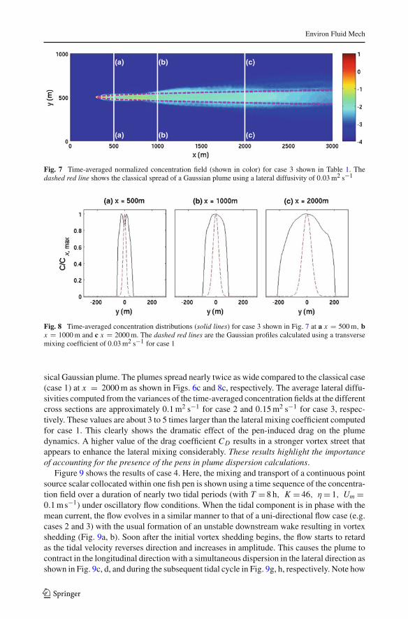
open channel test cases (cases 2 through 4). In an effort to understand the influence ofblockage introduced by the pens, we ran an ‘offshore case’ without accounting for the dragfrom the pens. For this case, it is clear from the concentration distribution shown in Fig. 12dthat the absence of drag results in less mixing compared to the ‘offshore case’ shown inFig. 12a, even though the overall plume distribution looks very similar. The peak concentra-tion is at least three times higher than the peak value for the ‘offshore base case’ as shownin Table 3 at t = 6T . This result in conjunction with the results of the channel flow testcases (cases 2–4) highlights the need to correctly account for the drag induced by the pensin predictive numerical models for water quality applications. An over prediction of the drag

Fig. 15 “Birds-eye-view” of the time history of the normalized concentration in the vicinity if two sets of 620 m diameter pens (depicted as white boxes) releasing a passive scalar at the edge of the coastal embaymentfor the ‘nearshore base case’ (case 9)

123

Environ Fluid Mech

Fig. 16 “Birds-eye-view” of the time history of the normalized concentration in the vicinity if two sets of6 20 m diameter pens (depicted as white boxes) releasing a passive scalar at the edge of the coastal embaymentat time t = 4T for a nearshore base case (case 9), b nearshore with strong tides case (case 10), c neashorewith wind case (case 11), respectively

(i.e. a higher drag coefficient) will result in a well mixed plume and on the other hand, underprediction (i.e. a lower drag coefficient) of the drag will imply poor mixing conditions.

3.2.5 Nearshore base case (case 9)

We have thus far presented results based on two sets of fish farms pens located along theedge of the embayment as shown in Fig. 1. For cases 9, 10 and 11, the southern facing farmin Fig. 1 was moved into the bay and closer to the channel incision. The concentration distri-butions of the plume for case 9 as seen in Fig. 15 indicate much higher concentrations closerto the coast compared to the ‘offshore base case’ (case 5). Figure 16 shows the concentrationdistributions at time t = 4T for all the nearshore cases (cases 9, 10 and 11, respectively). Asexpected, the concentration profiles along the coast as shown in Fig. 17 are at least an orderof magnitude higher than those for the ‘offshore base case’ (Fig. 13) especially at t = 6T .Time series of the concentrations at the three same locations shown for all offshore cases inFig. 14 are repeated here for all the nearshore cases (see Fig. 18). The relocation of the farmclose to the coast has reduced the concentration at the southern offshore boundary (Fig. 16a)while the concentration at the head of the channel incision has dramatically increased by upto two orders of magnitude (Fig. 16b).

3.2.6 Nearshore case with η = 2 (case 10)

The parameter η given in Eq. 6 determines the shape of the plume. In other words, it quanti-fies the effect of the tidal action to that of the mean current. A higher value of η signifies astronger tidal signal and allows for a stronger plume reversal. A simulation for the ‘nearshore

123

Environ Fluid Mech

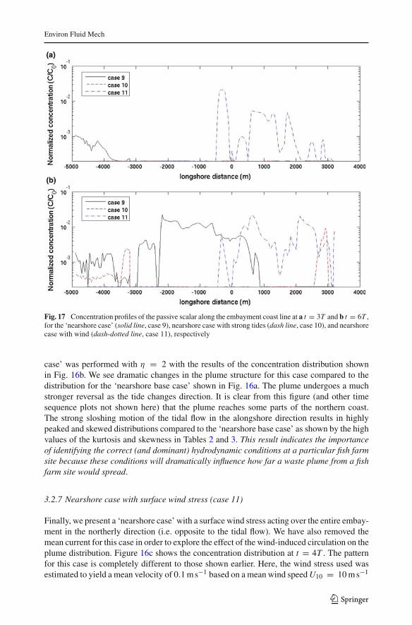
Fig. 17 Concentration profiles of the passive scalar along the embayment coast line at a t = 3T and b t = 6T ,for the ‘nearshore case’ (solid line, case 9), nearshore case with strong tides (dash line, case 10), and nearshorecase with wind (dash-dotted line, case 11), respectively

case’ was performed with η = 2 with the results of the concentration distribution shownin Fig. 16b. We see dramatic changes in the plume structure for this case compared to thedistribution for the ‘nearshore base case’ shown in Fig. 16a. The plume undergoes a muchstronger reversal as the tide changes direction. It is clear from this figure (and other timesequence plots not shown here) that the plume reaches some parts of the northern coast.The strong sloshing motion of the tidal flow in the alongshore direction results in highlypeaked and skewed distributions compared to the ‘nearshore base case’ as shown by the highvalues of the kurtosis and skewness in Tables 2 and 3. This result indicates the importanceof identifying the correct (and dominant) hydrodynamic conditions at a particular fish farmsite because these conditions will dramatically influence how far a waste plume from a fishfarm site would spread.

3.2.7 Nearshore case with surface wind stress (case 11)

Finally, we present a ‘nearshore case’ with a surface wind stress acting over the entire embay-ment in the northerly direction (i.e. opposite to the tidal flow). We have also removed themean current for this case in order to explore the effect of the wind-induced circulation on theplume distribution. Figure 16c shows the concentration distribution at t = 4T . The patternfor this case is completely different to those shown earlier. Here, the wind stress used wasestimated to yield a mean velocity of 0.1 m s−1 based on a mean wind speed U10 = 10 m s−1

123

Environ Fluid Mech

Fig. 18 Time series of concentration profiles of passive scalar at three different locations along the embaymentcoast for nearshore cases 9, 10, and 11, respectively

at a height of 10 m in the atmospheric boundary. Clearly, it is seen that the wind effect isdominant and tends to drive the distribution in a northward direction. This is accentuatedeven more when the tide reverses and the plume is dispersed more toward the northern endof the bay.

4 Conclusions

This study presents results from highly-resolved two-dimensional, depth-averaged numer-ical simulations of the mixing and transport of continuous point sources of waste from anarray of aquaculture pens modeled as porous cylinders. The results highlight the complex anddifferent dispersion patterns that occur under such flow conditions. In particular, the resultsfrom this study demonstrate the following key points:

– The mixing and dispersion of the pollutant field under oscillatory flow conditions withadded drag from the fish pens is very different from the classical uni-directional flowcase where a Gaussian plume spread occurs. Under oscillatory flow conditions, ourresults show plumes of waste with relatively high concentration occurring at considerabledistances from the source.

– The large scale effect of the Earth’s rotation does indeed influence the dispersion ofcontaminant plumes and should be accounted for in numerical models.

123

Environ Fluid Mech

– The local runoff from rivers and other tributaries should be taken into account in modelingthe plume dispersion in near-coastal environments.

– Accounting for the drag induced by the pens is important to accurately predict the levelof mixing in numerical models for water quality applications.

– It is necessary to identify the correct (and dominant) hydrodynamic conditions at a par-ticular fish farm site because these conditions will dramatically influence how far a wasteplume from a fish farm site would spread.

In addition, our work shows strong “non-Gaussian” behavior in that the spatial decay is notnecessarily exponential. This is highlighted by the statistics of the plume concentrations,which indicate highly peaked and skewed distributions and show that high concentrations ofthe scalar field can be found at significant distances from the source. The results also indicatepronounced spatio-temporal variability in the concentration fields and this spatio-temporalvariability is a strong function of the particular forcing parameters involved. Based on ourresults, “dilution as a solution to pollution” should not be prescribed for marine aquaculture,particularly in near-shore systems.

This study is a first step towards understanding the complex plume dispersion dynamicsin the vicinity of aquaculture farms in nearshore coastal waters. Further work using three-dimensional simulations, is required to gain key insights into the three-dimensional flowstructure that would occur in the close proximity of aquaculture pens. As an extension to thisstudy, we are performing highly-resolved, three-dimensional, nonhydrostatic simulations tounderstand the plume structure resulting from the complex flow pattern that occurs due toflow separation over and under submerged pens under stratified flow conditions. We also planto couple the flow model with a biological model that will allow for the prediction of otherwater quality parameters, such as dissolved oxygen and plankton concentrations. The use ofsuch models in the design of water quality regulations and the monitoring of wastes will bekey to ensuring an environmentally sound aquaculture industry.

Acknowledgments We thank the three anonymous reviewers for their constructive comments and recom-mendations which were very helpful in improving both the content and clarity of this paper. This work wassupported by Lenfest Ocean Program (Program director: Margaret Bowman). We gratefully acknowledge JerryHarris and Dennis Michael for providing time on the Stanford CEES cluster. SKV also gratefully acknowl-edges start-up support funds from the Department of Civil and Environmental Engineering (Head—ProfessorLuis Garcia) at Colorado State University.

References

1. Bowden KF (1967) Stability effects on turbulent mixing in tidal currents. Phys Fluids Supp 10:S278–S2802. California Fish and Game Code Sec.15008 (2006)3. California Regional Water Quality Control Board, Central Coast Region (2002) Waste Discharge Require-

ments NPDES General Permit for Discharges from Aquaculture and Aquariums. Order no. R3-2002-00764. Chatwin PC (1975) On the longitudinal dispersion of passive contaminant in oscillatory flow in tubes.

J Fluid Mech 71:513–5275. Crimaldi JP, Wiley MB, Koseff JR (2002) The relationship between mean and instantaneous structure in

turbulent passive scalar plumes. J Turbul 3(014). http://stacks.iop.org/JoT/3/0146. Delaux S, Stevens CL, Popinet S (2010) High-resolution computational fluid dynamics modelling of

suspended shellfish structures. Environ Fluid Mech. doi:10.1007/s10652-010-9183-y7. Fischer HB, List EJ, Koh RC, Imberger J, Brooks NH (1979) Mixing in inland and coastal waters.

Academic Press, San Diego8. Fringer OB, Gerritsen MG, Street RL (2006) An unstructured-grid, finite-volume, nonhydrostatic,

parallel coastal ocean simulator. Ocean Modell 14:139–1739. Helsley CE, Kim JW (2005) Mixing downstream of a submerged fish cage: a numerical study. IEEE J

Ocean Eng 30(1):12–19

123

Environ Fluid Mech

10. Hoyas S, Jiménez J (2006) Scaling of the velocity fluctuations in turbulent channel up to Reτ = 2003.Phys Fluids 18(7):011702

11. Jachec SJ, Fringer OB, Gerritsen MG, Street RL (2006) Numerical simulation of internal tides and theresulting energetics within Monterey Bay and the surrounding area. Geophys Res Lett 33. doi:10.1029/2006GL026314

12. Lau YL, Krishnappan BG (1977) Transverse dispersion in rectangular channels. J Hydraul Eng ASCE103(10):1173–1189

13. Naylor R (2006) Environmental safeguards for open ocean aquaculture. Natl Acad Sci Issues Sci Technol(Spring) 53–58

14. Naylor R, Burke M (2005) Aquaculture and ocean resources: raising tigers of the sea. Annu Rev EnvironResour 30:185–218

15. Plew DR, Spigel RH, Stevens CL, Nokes RI, Davidson MJ (2006) Stratified flow interactions with asuspended canopy. Environ Fluid Mech 6:519–539

16. Purnama A, Kay A (1999) Effluent discharge into tidal water: optimal or economic strategy?. Environ-metrics 10:601–624

17. Rummel AC, Socolofsky SA, Carmer CFv, Jirka GH (2005) Enhanced diffusion from a continuous pointsource in shallow free-surface flow with grid turbulence. Phys Fluids 17(7):075105

18. Smith R (1982) Contaminant dispersion in oscillatory flows. J Fluid Mech 114:379–39819. Stacey MT, Cowen EA, Powell TM, Dobbins E, Monismith SG, Koseff JR (2000) Plume dispersion in a

stratified, near-coastal flow: measurements and modeling. Cont Shelf Res 20(6):637–66320. Stevens C, Plew D, Hartstein N, Fredriksson D (2008) The physics of open-water shellfish aquaculture.

Aquacult Eng. 38(3):145–16021. Wang B, Fringer OB, Giddings SN, Fong DA (2009) High-resolution simulations of a macrotidal estuary

using SUNTANS. Ocean Modell 28(1–2):167–19222. Zhang Z, Fringer OB (2006) A numerical study of nonlinear internal wave generation in the luzon strait.

In: Proceedings of the 6th international symposium on stratified flows, pp 300–305

123