numerical analysis of earthquake response of an ultra-high ...numerical analysis of earthquake...
TRANSCRIPT
NHESSD1, 2319–2351, 2013
Numerical analysisof earthquake
response
W. X. Dong et al.
Title Page
Abstract Introduction
Conclusions References
Tables Figures
J I
J I
Back Close
Full Screen / Esc
Printer-friendly Version
Interactive Discussion
Discussion
Paper
|D
iscussionP
aper|
Discussion
Paper
|D
iscussionP
aper|
Nat. Hazards Earth Syst. Sci. Discuss., 1, 2319–2351, 2013www.nat-hazards-earth-syst-sci-discuss.net/1/2319/2013/doi:10.5194/nhessd-1-2319-2013© Author(s) 2013. CC Attribution 3.0 License.
EGU Journal Logos (RGB)
Advances in Geosciences
Open A
ccess
Natural Hazards and Earth System
Sciences
Open A
ccess
Annales Geophysicae
Open A
ccess
Nonlinear Processes in Geophysics
Open A
ccess
Atmospheric Chemistry
and Physics
Open A
ccess
Atmospheric Chemistry
and Physics
Open A
ccess
Discussions
Atmospheric Measurement
Techniques
Open A
ccess
Atmospheric Measurement
Techniques
Open A
ccess
Discussions
Biogeosciences
Open A
ccess
Open A
ccessBiogeosciences
Discussions
Climate of the Past
Open A
ccess
Open A
ccess
Climate of the Past
Discussions
Earth System Dynamics
Open A
ccess
Open A
ccess
Earth System Dynamics
Discussions
GeoscientificInstrumentation
Methods andData Systems
Open A
ccess
GeoscientificInstrumentation
Methods andData Systems
Open A
ccess
Discussions
GeoscientificModel Development
Open A
ccess
Open A
ccess
GeoscientificModel Development
Discussions
Hydrology and Earth System
Sciences
Open A
ccess
Hydrology and Earth System
Sciences
Open A
ccess
Discussions
Ocean Science
Open A
ccess
Open A
ccess
Ocean ScienceDiscussions
Solid Earth
Open A
ccess
Open A
ccess
Solid EarthDiscussions
The Cryosphere
Open A
ccess
Open A
ccess
The CryosphereDiscussions
Natural Hazards and Earth System
Sciences
Open A
ccess
Discussions
This discussion paper is/has been under review for the journal Natural Hazards and EarthSystem Sciences (NHESS). Please refer to the corresponding final paper in NHESS if available.
Numerical analysis of earthquakeresponse of an ultra-highearth-rockfill damW. X. Dong, W. J. Xu, Y. Z. Yu, and H. Lv
Department of Hydraulic Engineering, Tsinghua University, Beijing, China
Received: 18 April 2013 – Accepted: 10 May 2013 – Published: 28 May 2013
Correspondence to: Y. Z. Yu ([email protected])
Published by Copernicus Publications on behalf of the European Geosciences Union.
2319
NHESSD1, 2319–2351, 2013
Numerical analysisof earthquake
response
W. X. Dong et al.
Title Page
Abstract Introduction
Conclusions References
Tables Figures
J I
J I
Back Close
Full Screen / Esc
Printer-friendly Version
Interactive Discussion
Discussion
Paper
|D
iscussionP
aper|
Discussion
Paper
|D
iscussionP
aper|
Abstract
Failure of high earth dams under earthquake may cause disastrous economic damageand loss of lives. It is necessary to conduct seismic safety assessment, and numer-ical analysis is an effective way. Solid-fluid interaction has a significant influence onthe dynamic responses of geotechnical materials, which should be considered in the5
seismic analysis of earth dams. The initial stress field needed for dynamic computationis often obtained from postulation, without considering the effects of early constructionand reservoir impounding. In this study, coupled static analyses are conducted to simu-late the construction and impounding of an ultra-high earth rockfill dam in China. Thenbased on the initial static stress field, dynamic response of the dam is studied with fully10
coupled nonlinear method. Results show that excess pore water pressure accumulatesgradually with earthquake and the maximum value occurs at the bottom of core. Accel-eration amplification reaches the maximum at the crest as a result of whiplash effect.Horizontal and vertical permanent displacements both reach the maximum values atthe dam crest.15
1 Introduction
With the development of construction technology and a better understanding of theearth-rockfill dams’ mechanism (Yasuda and Matsumoto, 1993; Hunter and Fell, 2003;Soroush and Jannatiaghdam, 2012), high earth-rockfill dams have become a morecompetitive type of dams. A number of high core earth dams and concrete faced rockfill20
dams (CFRDs) with heights of more than 200 ∼ 300 m are being under constructionor to be built in Southwest China located in the Himalayas seismic belt with heavypotentially seismic activity.
Failures of earth dams, especially for high earth dams with a height more than 200 m,may cause catastrophic economic damage and loss of lives. Among these failures,25
earthquake attack is one of the major causes. In general, the principal failures induced
2320
NHESSD1, 2319–2351, 2013
Numerical analysisof earthquake
response
W. X. Dong et al.
Title Page
Abstract Introduction
Conclusions References
Tables Figures
J I
J I
Back Close
Full Screen / Esc
Printer-friendly Version
Interactive Discussion
Discussion
Paper
|D
iscussionP
aper|
Discussion
Paper
|D
iscussionP
aper|
by earthquake attack can be classified as sliding failure, liquefaction failure, longitudi-nal cracks, transverse cracks, and piping failure (Chen, 1995). Numerical computationbased on constitutive model of geotechnical materials is one of the effective ways toconduct seismic analyses and seismic safety assessment.
Earth dams are complicated nonhomogeneous geotechnical structures composed5
of different materials such as rockfill and clayey soils. This results in great difficulty toanalyse and predict the responses of earth dams under various conditions, such asconstruction, reservoir impounding and earthquake attacks (Costa and Alonso, 2009;Seo and Ha, 2009). Therefore, existing theories and numerical analyses of earth-rockfilldams include many simplifying assumptions (Prevost et al., 1985).10
Pseudo static method (Seed and Martin, 1966) is largely used in the numerical anal-yses to assess the seismic response of earth dams. In this approach, seismic effecton dam body is considered with an equivalent static force, which is the product of soilmass multiplied by a seismic coefficient, and soil is assumed as rigid-perfectly plasticbehaving.15
Newmark (Newmark, 1965) presented the important concept that the seismic sta-bility of slopes is more important rather than the traditional factor of safety, and heproposed a double integration method to compute the permanent displacement undercyclic loading, which is based on the concept of analyses of a rigid block sliding ona plane. Once the acceleration exceeds the “yield acceleration”, permanent displace-20
ment can be obtained by double integrating the acceleration.Up to now, most numerical earthquake response analyses of earth-rockfill dams
were conducted using equivalent linear models, in which shear modulus and dampingratio are obtained by iterative procedure (Abdel-Ghaffar and Scott, 1979; Mejia et al.,1982). Cascone and Rampello (2003) evaluated the seismic stability of an earth dam25
via the decoupled displacement analysis to compute the earthquake-induced displace-ments.
Parish et al. (2009) performed a study of the seismic response of a simplified typicalearth dam using the FLAC3D software. Non-associated Mohr–Coulomb criterion was
2321
NHESSD1, 2319–2351, 2013
Numerical analysisof earthquake
response
W. X. Dong et al.
Title Page
Abstract Introduction
Conclusions References
Tables Figures
J I
J I
Back Close
Full Screen / Esc
Printer-friendly Version
Interactive Discussion
Discussion
Paper
|D
iscussionP
aper|
Discussion
Paper
|D
iscussionP
aper|
adopted to describe the behaviour of both shells and core of the earth dam. Theiranalyses showed that plasticity should be considered in the analysis of the seismicresponse of the dam, as it leads to a decrease in the natural frequency of the dam,which could significantly affect the seismic response of the dam. However, this studydid not consider the fluid-skeleton interaction, which should have a significant influence5
on the seismic response of earth dams.Siyahi and Arslan (2008) studied the dynamic behaviour and earthquake resistance
of Alibey earth dam located in Turkey by adopting the OpenSees software (Open Sys-tem for Earthquake Engineering Simulation) (2000). Elastoplastic constitutive modelsof soils such as pressure dependent and independent multi-yield materials were imple-10
mented in the analyses. They obtained the permanent displacements and concludedthat the liquefaction effect is not significant.
However, so far, application of solid-fluid coupled elasto-plastic dynamic analyses insafety assessment of earth-rockfill dams is not much. Furthermore, the initial stressfield needed for dynamic computation is often provided without considering the effects15
of early construction and reservoir impounding.In this work, the static and dynamic responses of Nuozhadu high earth-rockfill dam
have been studied by solid-fluid coupled nonlinear method, since solid-fluid interactionhas a significant influence on the behaviour of earth dams. First, the dam site anddetailed design data are introduced. The adopted numerical analysis method and soil20
constitutive model parameters are presented.In the static analysis, the practical construction was simulated. Then, reservoir im-
pounding was simulated by conducting solid-fluid coupled analysis.At last, the coupled nonlinear dynamic analyses were conducted based on the initial
stress field obtained from the preceding computation. The acceleration component of25
the El Centro 1940 earthquake was chosen as seismic motion. The excess pore waterpressure, acceleration responding, and permanent displacements induced by seismicmove are presented and analysed.
2322
NHESSD1, 2319–2351, 2013
Numerical analysisof earthquake
response
W. X. Dong et al.
Title Page
Abstract Introduction
Conclusions References
Tables Figures
J I
J I
Back Close
Full Screen / Esc
Printer-friendly Version
Interactive Discussion
Discussion
Paper
|D
iscussionP
aper|
Discussion
Paper
|D
iscussionP
aper|
2 Background
2.1 Nuozhadu dam
Nuozhadu hydropower station is located in the Lancang River which is also namedMekong River in the downstream, in Yunnan Province, China, as shown in Fig. 1.The installed capacity of the power-station is 5850 MW. The most important part of5
Nuozhadu project is an ultra-high earth-rockfill dam with a height of 261.5 m, which isthe highest earth-rockfill dam in China and the fourth highest in the world. The reservoirhas a storage capacity of 237.0×10⁸m3, with the normal storage water level of 812.5 m(Fig. 2b).
Figure 2 shows the material zoning and construction stages of the maximum cross10
section. The elevation of the earth core bottom and the crest of the dam are 562.6 mand 824.1 m, respectively. The dam crest has a longitudinal length of 630 m with a widthof 18 m. The upstream and downstream slopes are at 1.9 : 1 and 1.8 : 1, respectively.The dam body is composed of several different types of materials. The shells of up-stream and downstream are composed of decomposed rock materials. Anti-seepage15
material in the earth core is clay mixed with gravel. Adding gravel to the clay can im-prove the strength of core and reduce the arching effect between shells and earth core.The gravel material consists of fresh crushed stone of breccia and granite with a maxi-mum diameter of 150 mm. In addition to these, fine rockfill and filter materials are filledagainst the earth core to prevent the fine particle from being washed away.20
The dam construction was started in 2008, and was completed at the end of 2012.Figure 1c shows the construction site on the dam crest. Figure 2b demonstrates thepractical construction process.
2.2 Numerical analyses method
Since solid-fluid interaction plays a significant role in the behaviour of earth dams25
during impounding and earthquake, coupled method was adopted in the work. The
2323
NHESSD1, 2319–2351, 2013
Numerical analysisof earthquake
response
W. X. Dong et al.
Title Page
Abstract Introduction
Conclusions References
Tables Figures
J I
J I
Back Close
Full Screen / Esc
Printer-friendly Version
Interactive Discussion
Discussion
Paper
|D
iscussionP
aper|
Discussion
Paper
|D
iscussionP
aper|
solid-fluid interaction consists of two mechanical effects. First, changes in pore pres-sure will affect the response of the solid according to the principle of effective stress.Second, changes in mechanical volume will also affect the pore pressure.
Governing differential equations to describe the interaction between soil and waterinclude constitutive laws, balance law, transport law, and compatibility equations below5
(Itasca Consulting Group, 2005).The constitutive response for the porous solid has the form
Xσi j +α
∂p∂tδi j = H(σi j ,ξi j − ξTij ,κ). (1)
whereXσi j is the co-rotational stress rate, p is the pore pressure, H is the functional
form of the constitutive law, κ is a history parameter, δi j is the Kronecher delta, and ξi j10
is the strain rate.The constitutive law for fluid content is related to change in pore pressure, p, satura-
tion, s, and mechanical volumetric strains, ε, as
1M∂p∂t
+ns∂s∂t
=1s∂ζ∂t
−α∂ε∂t
. (2)
where M is Biot modulus, n is the porosity, α is Biot coefficient and ζ is the variation of15
fluid content.The fluid mass balance maybe expressed as
−qi ,i +qv =∂ζ∂t
. (3)
where qv is the volumetric fluid source intensity.The fluid transport is described by Darcy’s law. For a homogeneous, isotropic solid20
and constant fluid density, this law is given in the form
qi = −ki l k̂(s)[p−ρfxjgj ],l . (4)2324
NHESSD1, 2319–2351, 2013
Numerical analysisof earthquake
response
W. X. Dong et al.
Title Page
Abstract Introduction
Conclusions References
Tables Figures
J I
J I
Back Close
Full Screen / Esc
Printer-friendly Version
Interactive Discussion
Discussion
Paper
|D
iscussionP
aper|
Discussion
Paper
|D
iscussionP
aper|
where qi is the specific discharge vector, k is the tensor of absolute mobility coefficientof the medium, k̂(s) is the relative mobility coefficient, ρf is the fluid density, and gj isthe component of the gravity vector.
And the relation between strain rate and velocity gradient is
ξi j =12
[vi ,j + vj ,i ]. (5)5
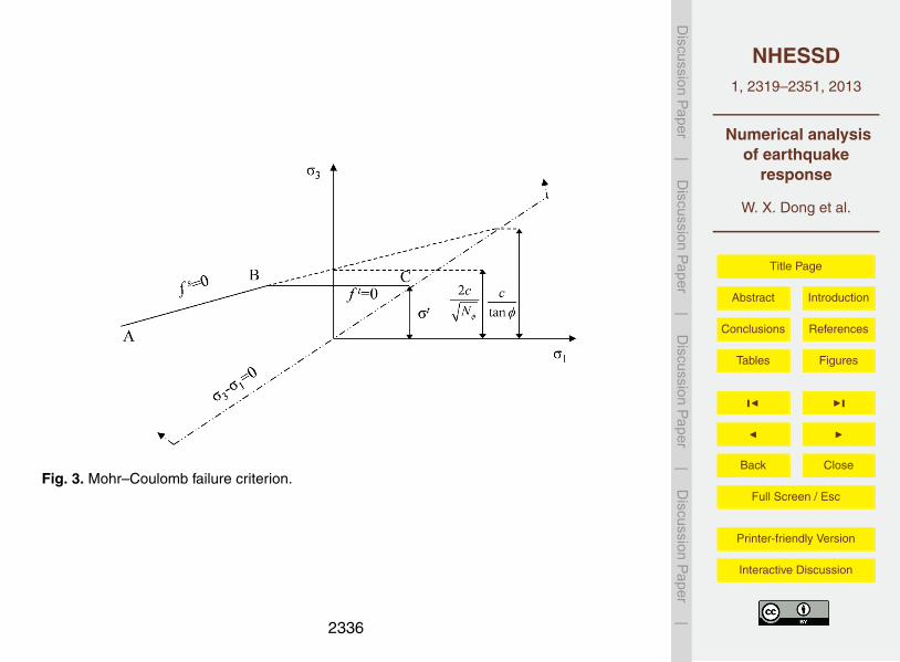
The Mohr–Coulomb model is the conventional model used to represent shear failurein soils and rocks. The failure criterion used in the constitutive model is a compositeMohr–Coulomb criterion with tension cut-off, which can be represented in the σ1 −σ3plane, as illustrated in Fig. 3.
The failure envelope f (σ1, σ3) = 0 is defined from point A to B by the Mohr–Coulomb10
failure criterion f s = 0 which can be derived from the classic form τf = σ tanΦ+c andfrom B to C by a tension failure criterion f t = 0
f s = σ1 −σ3Nφ +2c√Nφ, f t = σ3 −σ t, (6)
where φ is the friction angle, c, the cohesion, σt, the tensile strength, and Nφ = (1+sinΦ)/(1− sinφ).15
The potential function is described by means of two functions, gs and gt, used to de-fine shear plastic flow and tensile plastic flow, respectively. The function gs correspondsto a non-associated law and has the form
gs = σ1 −σ3Nψ . (7)
where ψ is the dilation angle and Nψ = (1+ sinψ)/(1− sinψ).20
The function gt corresponds to an associated flow rule and is written as
gt = −σ3. (8)
2325
NHESSD1, 2319–2351, 2013
Numerical analysisof earthquake
response
W. X. Dong et al.
Title Page
Abstract Introduction
Conclusions References
Tables Figures
J I
J I
Back Close
Full Screen / Esc
Printer-friendly Version
Interactive Discussion
Discussion
Paper
|D
iscussionP
aper|
Discussion
Paper
|D
iscussionP
aper|
2.3 Numerical model and parameters
The numerical analyses were performed by the effective stress analysis to simulate theperformance of the dam during construction stage and under earthquake action.
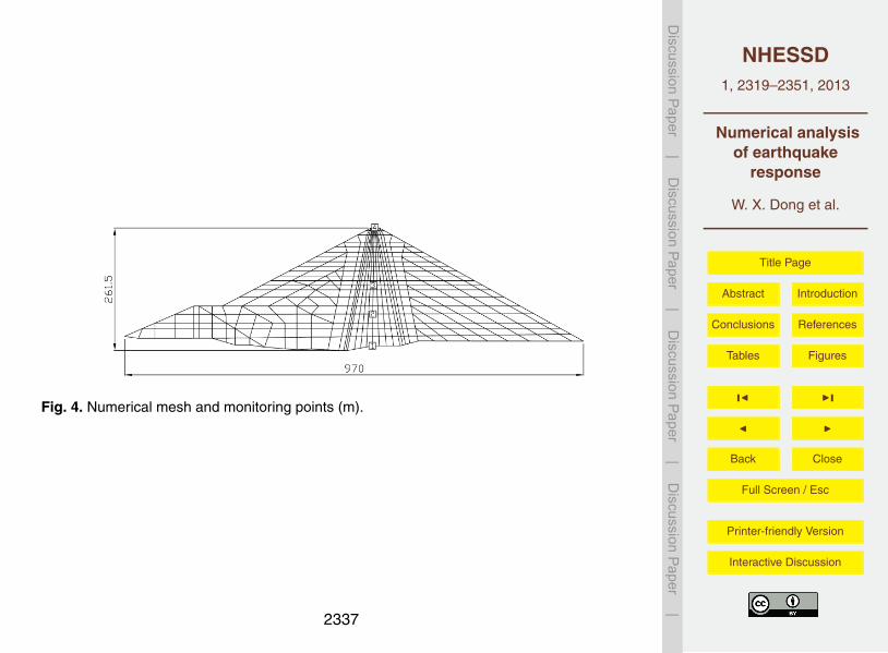
Figure 4 shows the mesh of the maximum cross section of the dam according to thematerial zoning and construction stage (see Fig. 2). There are 648 quadrilateral and5
triangular elements and 682 nodes.Geotechnical properties used in the analyses are presented in Table 1 for earth
dam materials. The friction angle and cohesion were determined through conventionaltriaxial test. The Young’s moduli were chosen more close to reality.
Numerical analyses presented in this study were performed by using the finite dif-10
ferential code FLAC3D, which is based on a continuum finite difference discretizationusing the Fast Lagrangian Approach.
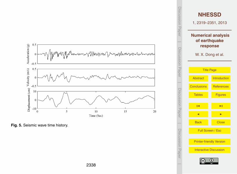
Seismic loading was input at the model base as a stress history excitation. In thestudy, El Centro earthquake was chosen as the horizontal acceleration and verticalacceleration by multiplying a factor of 2/3. The maximum acceleration occurs at 2.3 s15
with a value of 0.36 g. Velocity and displacement histories were obtained by integratingthe acceleration history (see Fig. 5). The local damping was applied in the dynamicsimulation with a value of 0.05.
The velocity history is transformed into stress history using the formulas as
σn = 2ρCpvn, σs = 2ρCsvs. (9)20
where ρ is soil mass density, σn and σs are applied normal stress and shear stress, vnand vs are input normal and shear velocities, Cp and Cs are the speeds of p wave ands wave propagating through medium given by
Cp =√
(K +4G/3)/ρ, Cs =√G/ρ. (10)
Viscous lateral boundary was applied to the model in order to prevent spurious re-25
flections of outward propagating waves from artificial boundaries. Free field boundarywas set in parallel with the main-grid.
2326
NHESSD1, 2319–2351, 2013
Numerical analysisof earthquake
response
W. X. Dong et al.
Title Page
Abstract Introduction
Conclusions References
Tables Figures
J I
J I
Back Close
Full Screen / Esc
Printer-friendly Version
Interactive Discussion
Discussion
Paper
|D
iscussionP
aper|
Discussion
Paper
|D
iscussionP
aper|
3 Static analysis
In order to conduct dynamic analysis, an initial stress field is needed. In this study,Mohr–Coulomb model was used to provide initial stress field. Since the real initialstress field has a significant influence on the seismic behaviour of the dam, practicalconstruction process was simulated according to the design (as shown in Fig. 2).5
3.1 Construction stage
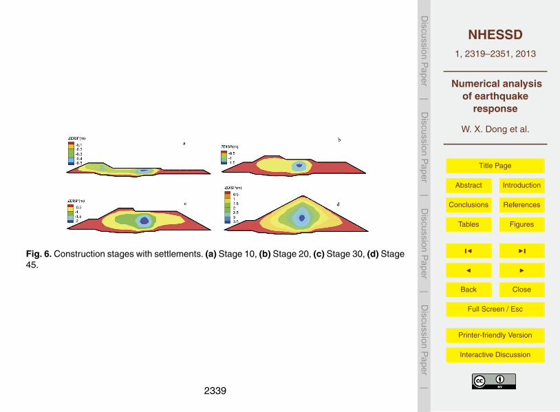
In the static analysis, staged construction was simulated by applying the null modelin FLAC3D. Forty five stages were divided according to the practical construction from2008 to 2012. Figure 6 shows the evolution of vertical displacement during constructionstage, from which we can see that the maximum vertical displacement occurred in the10
middle of earth core.Figure 7 presents the displacement and stress distributions when the dam construc-
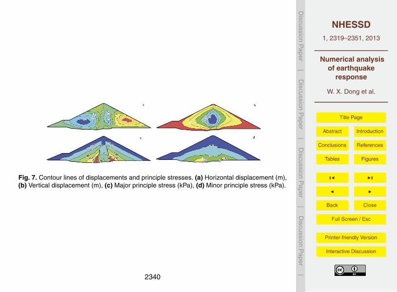
tion is completed. The largest settlement occurred in the middle of earth core witha value of about 3.72 m, which is slightly larger than the monitoring value of 3.55 m dueto the three dimensional effect. The monitoring value was obtained from the electro-15
magnetic settlement rings buried in the middle of earth core during construction. Largehorizontal displacements concentrated in the upstream and downstream shells witha maximum value of about 0.35 m. Because of the big differences of moduli betweenrockfill materials and clay, there exists obvious arching effect in the core wall, as shownin Fig. 7c.20
3.2 Reservoir impounding
Then, reservoir impounding was simulated by conducting solid-fluid coupled analyses.The normal storage level of 812.5 m was applied on the upstream slope, as shown inFig. 8. Earth core and dam shells with filter materials were set with different permeabil-ity coefficients, respectively (as shown in Table 1). The result shows that contour line25
2327
NHESSD1, 2319–2351, 2013
Numerical analysisof earthquake
response
W. X. Dong et al.
Title Page
Abstract Introduction
Conclusions References
Tables Figures
J I
J I
Back Close
Full Screen / Esc
Printer-friendly Version
Interactive Discussion
Discussion
Paper
|D
iscussionP
aper|
Discussion
Paper
|D
iscussionP
aper|
of pore pressure dropped sharply in the earth core, which proves the effectiveness ofthe earth core in anti-seepage.
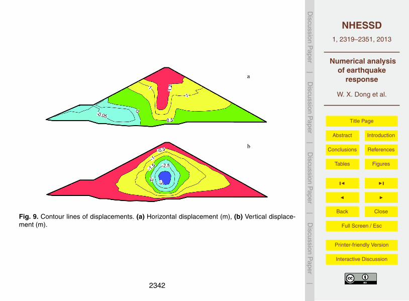
Figure 9 gives the displacements distribution after reservoir impounding. Comparedwith the analyses results of construction completion, horizontal displacement devel-oped toward downstream due to the water pressure applied on the upstream slope.5
As a result of reservoir storage, soils suffered an upward buoyant force, which resultedin the decrease of settlement without considering the wetting deformation of rockfillmaterials.
4 Dynamic analysis
Coupled solid-fluid dynamic analysis was conducted based on the initial stress field10
obtained from the preceding computation. Without empirical formulas for computingpermanent displacements and accumulated excess pore water pressure like traditionalequivalent linear method (Seed, 1966; Finn et al., 1977), nonlinear coupled dynamicanalysis can give those results directly.
4.1 Seismic wave input validation15
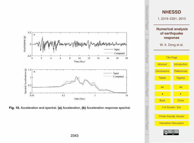
The N–S component of the El Centro 1940 earthquake was chosen as ground motionwith a 20 s duration time, as given in Fig. 5. The earthquake wave was applied to thedam in the upstream-downstream direction, and in the vertical direction multiplied by2/3. To verify the correctness of seismic wave input, acceleration time history wasrecorded at the model base, as shown in Fig. 10a. Furthermore, acceleration response20
spectral were obtained and compared in Fig. 10b. As shown in the figure, we can seethat the computed acceleration was quite close to the input acceleration.
2328
NHESSD1, 2319–2351, 2013
Numerical analysisof earthquake
response
W. X. Dong et al.
Title Page
Abstract Introduction
Conclusions References
Tables Figures
J I
J I
Back Close
Full Screen / Esc
Printer-friendly Version
Interactive Discussion
Discussion
Paper
|D
iscussionP
aper|
Discussion
Paper
|D
iscussionP
aper|
4.2 Result and analyses
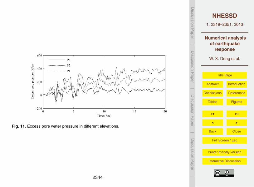
Permeability coefficient of the earth core was so small that pore water pressure cannotdissipate during the earthquake. Solid-fluid coupled analysis can give the accumulationprocess of excess pore water pressure. Figures 11 and 12 present the recorded excesspore pressure in the core center at different elevations (see monitoring points in Fig. 4)5
and different times, respectively.As shown in Fig. 11, the excess pore water pressure changed with the earthquake
action and accumulated gradually. The maximum excess pore pressure occurred at thebottom of core, as excess pore pressure in the middle of the core bottom was the mostdifficult to dissipate.10
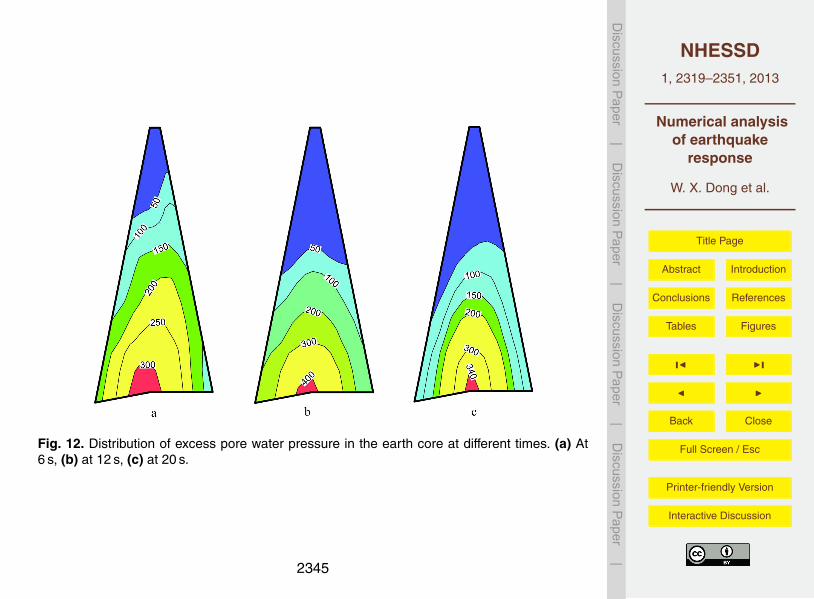
The distribution of excess pore pressure varied with time, as presented in Fig. 12.As we can see, the distribution of excess pore pressure varied with earthquake actionand the major excess pore pressure concentrates in the bottom of the core.
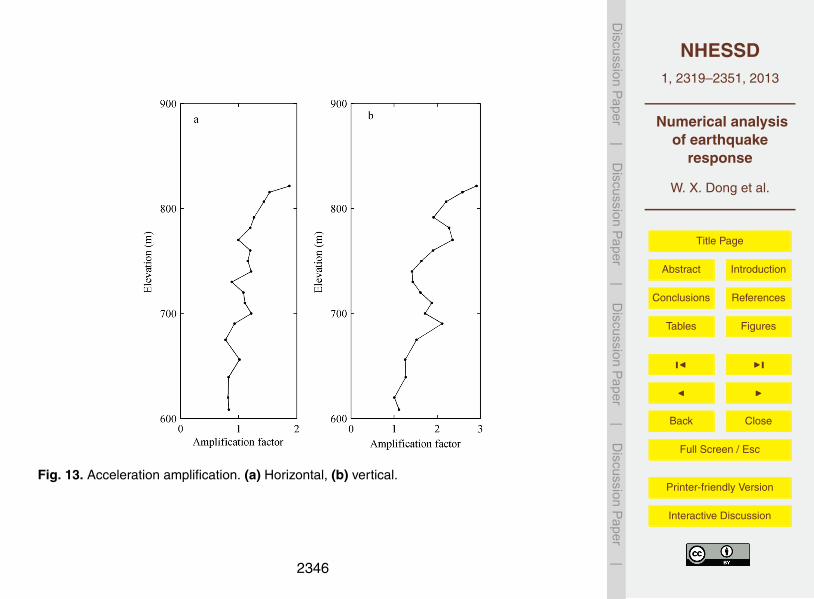
The acceleration amplification along the dam axis is presented in Fig. 13, where theacceleration amplification was defined as the ratio of the maximum recorded accelera-15
tion to the maximum input acceleration. As the figures shown, the amplification factorsincreased with elevation with a maximum value of 1.87 in the horizontal direction and2.91 for vertical direction. And it can be observed that the amplification factor increasedsharply near the crest of dam due to the whiplash effect (Gazetas, 1987).
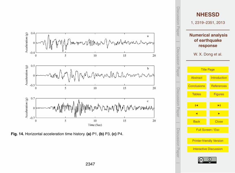
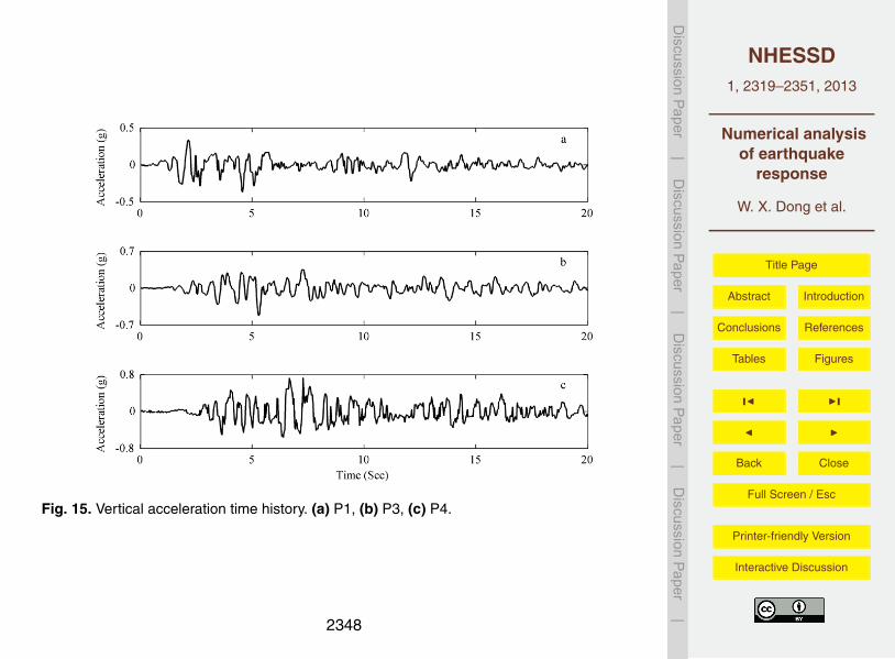
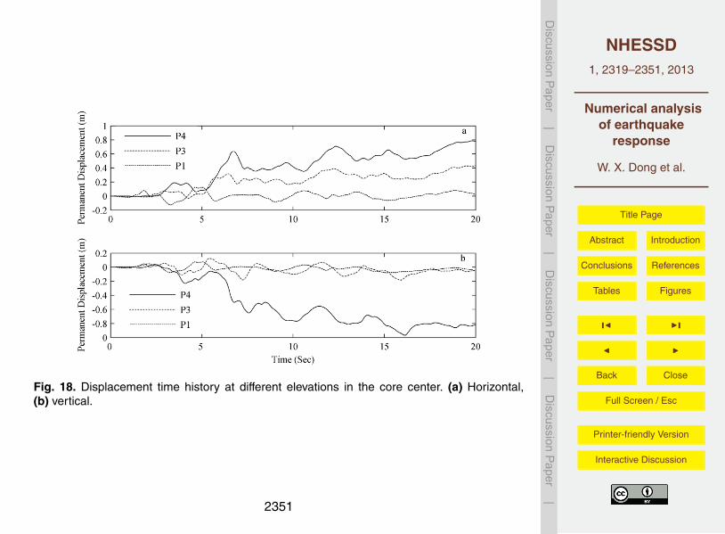
Time histories of acceleration at different elevations were monitored (see monitoring20
points in Fig. 4), as shown in Figs. 14 and 15. The maximum acceleration increasedwith elevations, and showed a delayed effect. The maximum accelerations occurred at2.1 s, 5.6 s, and 6.8 s, respectively.
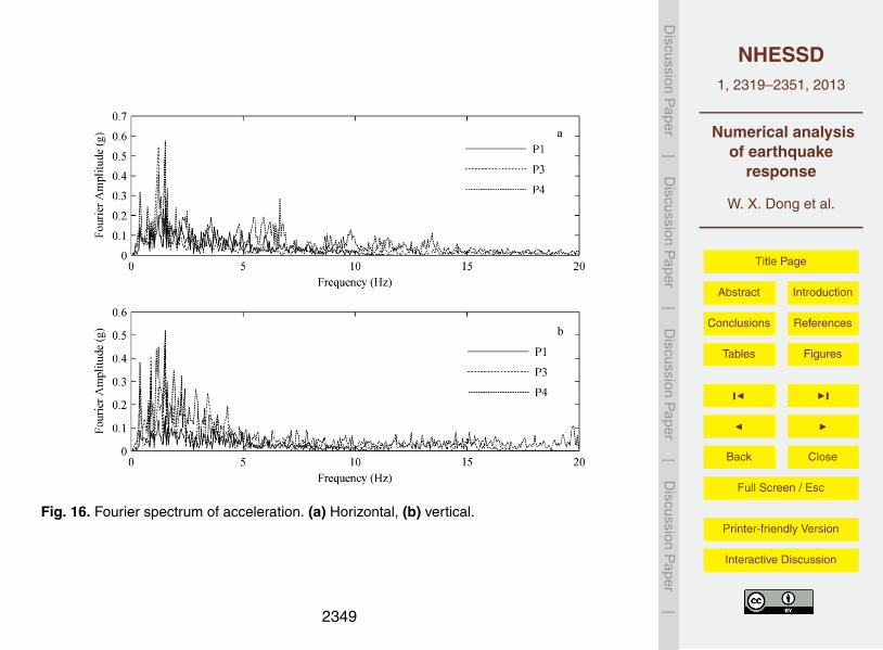
Figure 16 shows the Fourier amplitude spectrum of accelerations at different eleva-tions. It is shown that the amplifier of acceleration components mainly concentrated25
in the lower frequency ranging from 0.4 Hz to 2.0 Hz and 0.4 Hz to 3.4 Hz for horizon-tal and vertical acceleration, respectively. This indicates that the components of input
2329
NHESSD1, 2319–2351, 2013
Numerical analysisof earthquake
response
W. X. Dong et al.
Title Page
Abstract Introduction
Conclusions References
Tables Figures
J I
J I
Back Close
Full Screen / Esc
Printer-friendly Version
Interactive Discussion
Discussion
Paper
|D
iscussionP
aper|
Discussion
Paper
|D
iscussionP
aper|
earthquake whose dominant frequency was close to the natural frequency of the damare amplified significantly due to resonance.
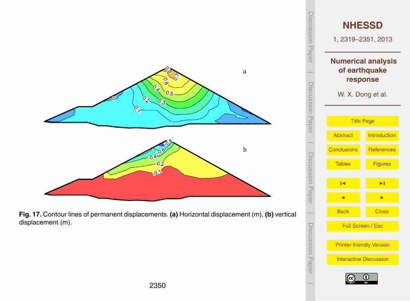
The permanent horizontal and vertical displacements induced by seismic move arepresented in Figs. 17 and 18. As seen from the figures, no matter horizontal or verticalpermanent displacements, they reached the maximum value at the crest with 0.83 m5
and 0.84 m, respectively. As a result, special attention should be paid to the design andconstruction of the dam crest, especially for high earth dams such as Nuozhadu highearth-rockfill dam.
In summary, solid-fluid coupled dynamic analysis can give a reasonable simulationresult of earth dams. Strong earthquake can bring seriously damage to the dam crest,10
which may lead to overtopping resulting in huge floods. Excess pore pressure gener-ated in the core can cause hydraulic fracture, which should be considered in the designof earth dams.
5 Conclusions
This paper includes analyses of the static and dynamic behaviour of an ultra-high earth-15
rockfill dam in the Southwest China. Mohr–Coulomb nonlinear elasto-plastic model wasadopted to describe the behaviour of dam materials.
In the static analysis, staged construction and reservoir impounding were simulated.Then based on the initial static stress field, dynamic response of the dam was stud-ied with fully-coupled nonlinear method. The dynamic behaviour of the dam during the20
earthquake was analysed, and the seismic characteristics of response were investi-gated.
The excess pore water pressure changed with the earthquake action and accumu-lated gradually. The maximum excess pore pressure occurred at the bottom of core.Acceleration amplification factors increased sharply in the upper part of the dam. As25
a result, special attention should be paid to the design and construction of the damcrest, especially for high earth dams such as Nuozhadu high earth-rockfill dam.
2330

NHESSD1, 2319–2351, 2013
Numerical analysisof earthquake
response
W. X. Dong et al.
Title Page
Abstract Introduction
Conclusions References
Tables Figures
J I
J I
Back Close
Full Screen / Esc
Printer-friendly Version
Interactive Discussion
Discussion
Paper
|D
iscussionP
aper|
Discussion
Paper
|D
iscussionP
aper|
Acknowledgements. This work was supported by National Nature Science Foundation of China(51179092) and State Key Laboratory of Hydroscience and Engineering Project (2012-KY-02and 2013-KY-4).
References
Abdel-Ghaffar, A. M. and Scott, R. F.: Shear moduli and damping factors of earth dam, J.5
Geotech. Geoenviron., 105, 1405–1426, 1979.Cascone, E. and Rampello, S.: Decoupled seismic analysis of an earth dam, Soil Dyn. Earthq.
Eng., 23, 349–365, 2003.Chen, M.: Response of an earth dam to spatially varying earthquake ground motion, Ph. D.
Dissertation, Civil and Environmental Engineering, Michigan State University, USA, 1995.10
Costa, L. and Alonso, E.: Predicting the behavior of an earth and rockfill dam under construc-tion, J. Geotech. Geoenviron., 135, 851–862, 2009.
Finn, W. D., Lee, K. W., and Martin, G. R.: An effective stress model for liquefaction, Electron.Lett., 103, 517–533, 1977.
Gazetas, G.: Seismic response of earth dams: some recent developments, Soil Dyn. Earthq.15
Eng., 6, 2–47, 1987.Hunter, G. and Fell, R.: Rockfill modulus and settlement of concrete face rockfill dams, J.
Geotech. Geoenviron., 129, 909–917, 2003.Itasca Consulting Group, Inc: FLAC (Fast Lagrangian Analysis of Continua), Version 3.0., Min-
neapolis, MN, 2005.20
McKenna, F., Fenves, G. L., and Scott, M. H.: Open system for earthquake engineering simu-lation, Univ. of California, Berkeley, Calif, USA, 2000.
Mejia, L. H., Seed, H. B., and Lysmer, J.: Dynamic analysis of earth dams in three dimen-sions, J. Geotech. Eng-ASCE, 108, 1586–1604, 1982.
Newmark, N. M.: Effects of earthquakes on dams and embankments, Geotechnique, 15, 139–25
160, 1965.Parish, Y., Sadek, M., and Shahrour, I.: Review Article: Numerical analysis of the seismic be-
haviour of earth dam, Nat. Hazards Earth Syst. Sci., 9, 451–458, doi:10.5194/nhess-9-451-2009, 2009.
2331
NHESSD1, 2319–2351, 2013
Numerical analysisof earthquake
response
W. X. Dong et al.
Title Page
Abstract Introduction
Conclusions References
Tables Figures
J I
J I
Back Close
Full Screen / Esc
Printer-friendly Version
Interactive Discussion
Discussion
Paper
|D
iscussionP
aper|
Discussion
Paper
|D
iscussionP
aper|
Prevost, J. H., Abdel-Ghaffar, A. M., and Lacy, S. J.: Nonlinear dynamic analyses of an earthdam, J. Geotech. Eng-ASCE, 111, 882–897, 1985.
Seed, H. B.: Earthquake-resistant design of earth dams, Can. Geotech. J., 4, 1–27, 1967.Seed, H. B. and Martin, G. R.: The seismic coefficient in earth dam design, J. Soil Mech. Found.
Div., 92, 25–58, 1966.5
Seo, M. W. and Ha, I. S.: Behavior of concrete-faced rockfill dams during initial impoundment, J.Geotech. Geoenviron., 135, 1070–1081, 2009.
Siyahi, B. and Arslan, H.: Nonlinear dynamic finite element simulation of Alibey earth dam,Environ. Geol., 54, 77–85, 2008.
Soroush, A. and Jannatiaghdam, R.: Behavior of rockfill materials in triaxial compression test-10
ing, Int. J. Civil Eng., 10, 153–161, 2012.Yasuda, N. and Matsumoto, N.: Dynamic deformation characteristics of sands and rockfill ma-
terials, Can. Geotech. J., 30, 747–757, 1993.
2332
NHESSD1, 2319–2351, 2013
Numerical analysisof earthquake
response
W. X. Dong et al.
Title Page
Abstract Introduction
Conclusions References
Tables Figures
J I
J I
Back Close
Full Screen / Esc
Printer-friendly Version
Interactive Discussion
Discussion
Paper
|D
iscussionP
aper|
Discussion
Paper
|D
iscussionP
aper|
Table 1. Material properties of earth dam soils.
Units RD1/RU1 RD2/RU2 RD3/RU3 F1 F2 Clay
Dry density kgm−3 2190 2310 2170 2000 2050 2120Young’s modulus MPa 100 100 100 80 80 25Poisson’s ratio – 0.3 0.3 0.3 0.3 0.3 0.3Cohesion kPa 141 114 106 127 105 73Friction angle Degree 40.8 39.0 42.8 40.2 39.4 27.1Dilation angle Degree 15.8 14.0 17.8 15.2 14.4 12.1Permeability coefficient cm s−1 1.0×10⁻¹ 1.0×10⁻¹ 1.0×10⁻¹ 1.0×10⁻¹ 1.0×10⁻¹ 1.0×10⁻⁶
2333
NHESSD1, 2319–2351, 2013
Numerical analysisof earthquake
response
W. X. Dong et al.
Title Page
Abstract Introduction
Conclusions References
Tables Figures
J I
J I
Back Close
Full Screen / Esc
Printer-friendly Version
Interactive Discussion
Discussion
Paper
|D
iscussionP
aper|
Discussion
Paper
|D
iscussionP
aper|
Fig. 1. Nuozhadu dam. (a) Nuozhadu dam location, (b) Project blueprint, (c) Nuozhadu damunder construction, (d) Dam site geomorphology
16
Fig. 1. Nuozhadu dam. (a) Nuozhadu dam location, (b) Project blueprint, (c) Nuozhadu damunder construction, (d) Dam site geomorphology.
2334
NHESSD1, 2319–2351, 2013
Numerical analysisof earthquake
response
W. X. Dong et al.
Title Page
Abstract Introduction
Conclusions References
Tables Figures
J I
J I
Back Close
Full Screen / Esc
Printer-friendly Version
Interactive Discussion
Discussion
Paper
|D
iscussionP
aper|
Discussion
Paper
|D
iscussionP
aper|
Fig. 2. Maximum cross section with material zoning and construction stage.
17
Fig. 2. Maximum cross section with material zoning and construction stage.
2335
NHESSD1, 2319–2351, 2013
Numerical analysisof earthquake
response
W. X. Dong et al.
Title Page
Abstract Introduction
Conclusions References
Tables Figures
J I
J I
Back Close
Full Screen / Esc
Printer-friendly Version
Interactive Discussion
Discussion
Paper
|D
iscussionP
aper|
Discussion
Paper
|D
iscussionP
aper|
Fig. 3. Mohr–Coulomb failure criterion.
18
Fig. 3. Mohr–Coulomb failure criterion.
2336
NHESSD1, 2319–2351, 2013
Numerical analysisof earthquake
response
W. X. Dong et al.
Title Page
Abstract Introduction
Conclusions References
Tables Figures
J I
J I
Back Close
Full Screen / Esc
Printer-friendly Version
Interactive Discussion
Discussion
Paper
|D
iscussionP
aper|
Discussion
Paper
|D
iscussionP
aper|
Fig. 4. Numerical mesh and monitoring points (m).
19
Fig. 4. Numerical mesh and monitoring points (m).
2337
NHESSD1, 2319–2351, 2013
Numerical analysisof earthquake
response
W. X. Dong et al.
Title Page
Abstract Introduction
Conclusions References
Tables Figures
J I
J I
Back Close
Full Screen / Esc
Printer-friendly Version
Interactive Discussion
Discussion
Paper
|D
iscussionP
aper|
Discussion
Paper
|D
iscussionP
aper|
Fig. 5. Seismic wave time history.
20
Fig. 5. Seismic wave time history.
2338
NHESSD1, 2319–2351, 2013
Numerical analysisof earthquake
response
W. X. Dong et al.
Title Page
Abstract Introduction
Conclusions References
Tables Figures
J I
J I
Back Close
Full Screen / Esc
Printer-friendly Version
Interactive Discussion
Discussion
Paper
|D
iscussionP
aper|
Discussion
Paper
|D
iscussionP
aper|
Fig. 6. Construction stages with settlements. (a) Stage 10, (b) Stage 20, (c) Stage 30, (d) Stage45.
21
Fig. 6. Construction stages with settlements. (a) Stage 10, (b) Stage 20, (c) Stage 30, (d) Stage45.
2339
NHESSD1, 2319–2351, 2013
Numerical analysisof earthquake
response
W. X. Dong et al.
Title Page
Abstract Introduction
Conclusions References
Tables Figures
J I
J I
Back Close
Full Screen / Esc
Printer-friendly Version
Interactive Discussion
Discussion
Paper
|D
iscussionP
aper|
Discussion
Paper
|D
iscussionP
aper|
Fig. 7. Contour lines of displacements and principle stresses. (a) Horizontal displacement (m),(b) Vertical displacement (m), (c) Major principle stress (kPa), (d) Minor principle stress (kPa).
22
Fig. 7. Contour lines of displacements and principle stresses. (a) Horizontal displacement (m),(b) Vertical displacement (m), (c) Major principle stress (kPa), (d) Minor principle stress (kPa).
2340

NHESSD1, 2319–2351, 2013
Numerical analysisof earthquake
response
W. X. Dong et al.
Title Page
Abstract Introduction
Conclusions References
Tables Figures
J I
J I
Back Close
Full Screen / Esc
Printer-friendly Version
Interactive Discussion
Discussion
Paper
|D
iscussionP
aper|
Discussion
Paper
|D
iscussionP
aper|
Fig. 8. Reservoir water level and contour lines of pore water pressure (kPa).
23
Fig. 8. Reservoir water level and contour lines of pore water pressure (kPa).
2341
NHESSD1, 2319–2351, 2013
Numerical analysisof earthquake
response
W. X. Dong et al.
Title Page
Abstract Introduction
Conclusions References
Tables Figures
J I
J I
Back Close
Full Screen / Esc
Printer-friendly Version
Interactive Discussion
Discussion
Paper
|D
iscussionP
aper|
Discussion
Paper
|D
iscussionP
aper|
Fig. 9. Contour lines of displacements. (a) Horizontal displacement (m), (b) Vertical displace-ment (m).
24
Fig. 9. Contour lines of displacements. (a) Horizontal displacement (m), (b) Vertical displace-ment (m).
2342
NHESSD1, 2319–2351, 2013
Numerical analysisof earthquake
response
W. X. Dong et al.
Title Page
Abstract Introduction
Conclusions References
Tables Figures
J I
J I
Back Close
Full Screen / Esc
Printer-friendly Version
Interactive Discussion
Discussion
Paper
|D
iscussionP
aper|
Discussion
Paper
|D
iscussionP
aper|
Fig. 10. Acceleration and spectral. (a) Acceleration, (b) Acceleration response spectral.
25
Fig. 10. Acceleration and spectral. (a) Acceleration, (b) Acceleration response spectral.
2343
NHESSD1, 2319–2351, 2013
Numerical analysisof earthquake
response
W. X. Dong et al.
Title Page
Abstract Introduction
Conclusions References
Tables Figures
J I
J I
Back Close
Full Screen / Esc
Printer-friendly Version
Interactive Discussion
Discussion
Paper
|D
iscussionP
aper|
Discussion
Paper
|D
iscussionP
aper|
Fig. 11. Excess pore water pressure in different elevations.
26
Fig. 11. Excess pore water pressure in different elevations.
2344
NHESSD1, 2319–2351, 2013
Numerical analysisof earthquake
response
W. X. Dong et al.
Title Page
Abstract Introduction
Conclusions References
Tables Figures
J I
J I
Back Close
Full Screen / Esc
Printer-friendly Version
Interactive Discussion
Discussion
Paper
|D
iscussionP
aper|
Discussion
Paper
|D
iscussionP
aper|
Fig. 12. Distribution of excess pore water pressure in the earth core at different times. (a) At6 s, (b) at 12 s, (c) at 20 s.
27
Fig. 12. Distribution of excess pore water pressure in the earth core at different times. (a) At6 s, (b) at 12 s, (c) at 20 s.
2345
NHESSD1, 2319–2351, 2013
Numerical analysisof earthquake
response
W. X. Dong et al.
Title Page
Abstract Introduction
Conclusions References
Tables Figures
J I
J I
Back Close
Full Screen / Esc
Printer-friendly Version
Interactive Discussion
Discussion
Paper
|D
iscussionP
aper|
Discussion
Paper
|D
iscussionP
aper|
Fig. 13. Acceleration amplification. (a) Horizontal, (b) vertical.
2346
NHESSD1, 2319–2351, 2013
Numerical analysisof earthquake
response
W. X. Dong et al.
Title Page
Abstract Introduction
Conclusions References
Tables Figures
J I
J I
Back Close
Full Screen / Esc
Printer-friendly Version
Interactive Discussion
Discussion
Paper
|D
iscussionP
aper|
Discussion
Paper
|D
iscussionP
aper|
Fig. 14. Horizontal acceleration time history. (a) P1, (b) P3, (c) P4.
2347
NHESSD1, 2319–2351, 2013
Numerical analysisof earthquake
response
W. X. Dong et al.
Title Page
Abstract Introduction
Conclusions References
Tables Figures
J I
J I
Back Close
Full Screen / Esc
Printer-friendly Version
Interactive Discussion
Discussion
Paper
|D
iscussionP
aper|
Discussion
Paper
|D
iscussionP
aper|
Fig. 15. Vertical acceleration time history. (a) P1, (b) P3, (c) P4.
2348
NHESSD1, 2319–2351, 2013
Numerical analysisof earthquake
response
W. X. Dong et al.
Title Page
Abstract Introduction
Conclusions References
Tables Figures
J I
J I
Back Close
Full Screen / Esc
Printer-friendly Version
Interactive Discussion
Discussion
Paper
|D
iscussionP
aper|
Discussion
Paper
|D
iscussionP
aper|
Fig. 16. Fourier spectrum of acceleration. (a) Horizontal, (b) vertical.
2349
NHESSD1, 2319–2351, 2013
Numerical analysisof earthquake
response
W. X. Dong et al.
Title Page
Abstract Introduction
Conclusions References
Tables Figures
J I
J I
Back Close
Full Screen / Esc
Printer-friendly Version
Interactive Discussion
Discussion
Paper
|D
iscussionP
aper|
Discussion
Paper
|D
iscussionP
aper|
Fig. 17. Contour lines of permanent displacements. (a) Horizontal displacement (m), (b) verticaldisplacement (m).
2350
NHESSD1, 2319–2351, 2013
Numerical analysisof earthquake
response
W. X. Dong et al.
Title Page
Abstract Introduction
Conclusions References
Tables Figures
J I
J I
Back Close
Full Screen / Esc
Printer-friendly Version
Interactive Discussion
Discussion
Paper
|D
iscussionP
aper|
Discussion
Paper
|D
iscussionP
aper|
Fig. 18. Displacement time history at different elevations in the core center. (a) Horizontal,(b) vertical.
2351