notes on differential forms lorenzosadun arxiv:1604 ... · notes on differential forms...
TRANSCRIPT
arX
iv:1
604.
0786
2v1
[m
ath.
AT
] 2
6 A
pr 2
016
Notes on Differential Forms
Lorenzo Sadun
Department of Mathematics, The University of Texas at Austin, Austin,
TX 78712

CHAPTER 1
Forms on Rn
This is a series of lecture notes, with embedded problems, aimed at students studying
differential topology.
Many revered texts, such as Spivak’s Calculus on Manifolds and Guillemin and Pollack’s
Differential Topology introduce forms by first working through properties of alternating ten-
sors. Unfortunately, many students get bogged down with the whole notion of tensors and
never get to the punch lines: Stokes’ Theorem, de Rham cohomology, Poincare duality, and
the realization of various topological invariants (e.g. the degree of a map) via forms, none
of which actually require tensors to make sense!
In these notes, we’ll follow a different approach, following the philosophy of Amy’s Ice
Cream:
Life is uncertain. Eat dessert first.
We’re first going to define forms on Rn via unmotivated formulas, develop some profi-
ciency with calculation, show that forms behave nicely under changes of coordinates, and
prove Stokes’ Theorem. This approach has the disadvantage that it doesn’t develop deep
intuition, but the strong advantage that the key properties of forms emerge quickly and
cleanly.
Only then, in Chapter 3, will we go back and show that tensors with certain (anti)symmetry
properties have the exact same properties as the formal objects that we studied in Chapters
1 and 2. This allows us to re-interpret all of our old results from a more modern perspective,
and move onwards to using forms to do topology.
1. What is a form?
On Rn, we start with the symbols dx1, . . . , dxn, which at this point are pretty much
meaningless. We define a multiplication operation on these symbols, denoted by a ∧, subject
to the condition
dxi ∧ dxj = −dxj ∧ dxi.
Of course, we also want the usual properties of multiplication to also hold. If α, β, γ are
arbitrary products of dxi’s, and if c is any constant, then
(α+ β) ∧ γ = α ∧ γ + β ∧ γ
3
4 1. FORMS ON Rn
α ∧ (β + γ) = α ∧ β + α ∧ γ
(α ∧ β) ∧ γ = α ∧ (β ∧ γ)
(cα) ∧ β = α ∧ (cβ) = c(α ∧ β)(1)
Note that the anti-symmetry implies that dxi ∧ dxi = 0. Likewise, if I = i1, . . . , ik is a
list of indices where some index gets repeated, then dxi1 ∧ · · · ∧ dxik = 0, since we can swap
the order of terms (while keeping track of signs) until the same index comes up twice in a
row. For instance,
dx1 ∧ dx2 ∧ dx1 = −dx1 ∧ dx1 ∧ dx2 = −(dx1 ∧ dx1) ∧ dx2 = 0.
• A 0-form on Rn is just a function.
• A 1-form is an expression of the form∑
i
fi(x)dxi, where fi(x) is a function and
dxi is one of our meaningless symbols.
• A 2-form is an expression of the form∑
i,j
fij(x)dxi ∧ dxj .
• A k-form is an expression of the form∑
I
fI(x)dxI , where I is a subset i1, . . . , ik
of 1, 2, . . . , n and dxI is shorthand for dxi1 ∧ · · · ∧ dxik .
• If α is a k-form, we say that α has degree k.
For instance, on R3
• 0-forms are functions
• 1-forms look like Pdx + Qdy + Rdz, where P , Q and R are functions and we are
writing dx, dy, dz for dx1, dx2, dx3.
• 2-forms look like Pdx ∧ dy + Qdx ∧ dz + Rdy ∧ dz. Or we could just as well write
Pdx ∧ dy −Qdz ∧ dx+Rdy ∧ dz.
• 3-forms look like fdx ∧ dy ∧ dz.
• There are no (nonzero) forms of degree greater than 3.
When working on Rn, there are exactly
(nk
)
linearly independent dxI ’s of degree k, and
2n linearly independent dxI ’s in all (where we include 1 = dxI when I is the empty list). If
I ′ is a permutation of I, then dxI′
= ±dxI , and it’s silly to include both fIdxI and fI′dx
I′
in our expansion of a k-form. Instead, one usually picks a preferred ordering of i1, . . . , ik
(typically i1 < i2 < · · · < ik) and restrict our sum to I’s of that sort. When working with
2-forms on R3, we can use dx ∧ dz or dz ∧ dz, but we don’t need both.
If α =∑
αI(x)dxI is a k-form and β =
∑
βJ(x)dxJ is an ℓ-form, then we define
α ∧ β =∑
I,J
αI(x)βJ(x)dxI ∧ dxJ .
2. DERIVATIVES OF FORMS 5
Of course, if I and J intersect, then dxI ∧ dxJ = 0. Since going from (I, J) to (J, I) involves
kℓ swaps, we have
dxJ ∧ dxI = (−1)kℓdxI ∧ dxJ ,
and likewise β ∧ α = (−1)kℓα ∧ β. Note that the wedge product of a 0-form (aka function)
with a k-form is just ordinary multiplication.
2. Derivatives of forms
If α =∑
I
αIdxI is a k-form, then we define the exterior derivative
dα =∑
I,j
∂αI(x)
∂xjdxj ∧ dxI .
Note that j is a single index, not a multi-index. For instance, on R2, if α = xydx + exdy,
then
dα = ydx ∧ dx+ xdy ∧ dx+ exdx ∧ dy + 0dy ∧ dy
= (ex − x)dx ∧ dy.(2)
If f is a 0-form, then we have something even simpler:
df(x) =∑ ∂f(x)
∂xjdxj,
which should look familiar, if only as an imprecise calculus formula. One of our goals is to
make such statements precise and rigorous. Also, remember that xi is actually a function on
Rn. Since ∂jx
i = 1 if i = j and 0 otherwise, d(xi) = dxi, which suggests that our formalism
isn’t totally nuts.
The key properties of the exterior derivative operator d are listed in the following
Theorem 2.1. (1) If α is a k-form and β is an ℓ-form, then
d(α ∧ β) = (dα) ∧ β + (−1)kα ∧ (dβ).
(2) d(dα) = 0. (We abbreviate this by writing d2 = 0.)
Proof. For simplicity, we prove this for the case where α = αIdxI and β = βJdx
J each
have only a single term. The general case then follows from linearity.
The first property is essentially the product rule for derivatives.
α ∧ β = αI(x)βJ (x)dxI ∧ dxJ
d(α ∧ β) =∑
j
∂j(αI(x)βJ(x))dxj ∧ dxI ∧ dxJ
=∑
j
(∂jαI(x))βJ (x)dxj ∧ dxI ∧ dxJ
6 1. FORMS ON Rn
+∑
j
αI(x)∂jβJ(x)dxj ∧ dxI ∧ dxJ
=∑
j
(∂jαI(x))dxj ∧ dxI ∧ βJ(x)dx
J
+(−1)k∑
j
αI(x)dxI ∧ ∂jβJ(x)dx
j ∧ dxJ
= (dα) ∧ β + (−1)kα ∧ dβ.(3)
The second property for 0-forms (aka functions) is just “mixed partials are equal”:
d(df) = d(∑
i
∂ifdxi)
=∑
j
∑
i
∂j∂ifdxj ∧ dxi
= −∑
i,j
∂i∂jfdxi ∧ dxj
= −d(df) = 0,(4)
where in the third line we used ∂j∂if = ∂i∂jf and dxi ∧ dxj = −dxj ∧ dxi. We then use the
first property, and the (obvious) fact that d(dxI) = 0, to extend this to k-forms:
d(dα) = d(dαI ∧ dxI)
= (d(dαI)) ∧ dxI − dαI ∧ d(dx
I)
= 0− 0 = 0.(5)
where in the second line we used the fact that dαI is a 1-form, and in the third line used the
fact that d(dαI) is d2 applied to a function, while d(dxI) = 0.
Exercise 1: On R3, there are interesting 1-forms and 2-forms associated with each vector
field ~v(x) = (v1(x), v2(x), v3(x)). (Here vi is a component of the vector ~v, not a vector in its
own right.) Let ω1~v = v1dx+ v2dy+ v3dz, and let ω2
~v = v1dy∧dz+ v2dz∧dx+ v3dx∧dy. Let
f be a function. Show that (a) df = ω1∇f , (b) dω
1~v = ω2
∇×~v, and (c) dω2~v = (∇·~v) dx∧dy∧dz,
where ∇, ∇× and ∇· are the usual gradient, curl, and divergence operations.
Exercise 2: A form ω is called closed if dω = 0, and exact if ω = dν for some other
form ν. Since d2 = 0, all exact forms are closed. On Rn it happens that all closed forms
of nonzero degree are exact. (This is called the Poincare Lemma). However, on subsets
of Rn the Poincare Lemma does not necessarily hold. On R2 minus the origin, show that
ω = (xdy − ydx)/(x2 + y2) is closed. We will soon see that ω is not exact.
3. PULLBACKS 7
3. Pullbacks
Suppose that g : X → Y is a smooth map, where X is an open subset of Rn and Y is
an open subset of Rm, and that α is a k-form on Y . We want to define a pullback form g∗α
on X . Note that, as the name implies, the pullback operation reverses the arrows! While g
maps X to Y , and dg maps tangent vectors on X to tangent vectors on Y , g∗ maps forms
on Y to forms on X .
Theorem 3.1. There is a unique linear map g∗ taking forms on Y to forms on X such
that the following properties hold:
(1) If f : Y → R is a function on Y , then g∗f = f g.
(2) If α and β are forms on Y , then g∗(α ∧ β) = (g∗α) ∧ (g∗β).
(3) If α is a form on Y , then g∗(dα) = d(g∗(α)). (Note that there are really two different
d’s in this equation. On the left hand side d maps k-forms on Y to (k + 1)-forms
on Y . On the right hand side, d maps k forms on X to (k + 1)-forms on X. )
Proof. The pullback of 0-forms is defined by the first property. However, note that
on Y , the form dyi is d of the function yi (where we’re using coordinates yi on Y and
reserving x’s for X). This means that g∗(dyi)(x) = d(yi g)(x) = dgi(x), where gi(x) is the
i-th component of g(x). But that gives us our formula in general! If α =∑
I
αI(y)dyI, then
(6) g∗α(x) =∑
I
αI(g(x))dgi1 ∧ dgi2 ∧ · · · ∧ dgik .
Using the formula (6), it’s easy to see that g∗(α ∧ β) = g∗(α) ∧ g∗(β). Checking that
g∗(dα) = d(g∗α) in general is left as an exercise in definition-chasing.
Exercise 3: Do that exercise!
An extremely important special case is where m = n = k. The n-form dy1 ∧ · · · ∧ dyn is
called the volume form on Rn.
Exercise 4: Let g is a smooth map from Rn to R
n, and let ω be the volume form on Rn.
Show that g∗ω, evaluated at a point x, is det(dgx) times the volume form evaluated at x.
Exercise 5: An important property of pullbacks is that they are natural. If g : U → V and
h : V →W , where U , V , and W are open subsets of Euclidean spaces of various dimensions,
then h g maps U →W . Show that (h g)∗ = g∗ h∗.
Exercise 6: Let U = (0,∞) × (0, 2π), and let V be R2 minus the non-negative x axis.
We’ll use coordinates (r, θ) for U and (x, y) for V . Let g(r, θ) = (r cos(θ), r sin(θ)), and let
h = g−1. On V , let α = e−(x2+y2)dx ∧ dy.
8 1. FORMS ON Rn
(a) Compute g∗(x), g∗(y), g∗(dx), g∗(dy), g∗(dx ∧ dy) and g∗α (preferably in that order).
(b) Now compute h∗(r), h∗(θ), h∗(dr) and h∗(dθ).
The upshot of this exercise is that pullbacks are something that you have been doing for
a long time! Every time you do a change of coordinates in calculus, you’re actually doing a
pullback.
4. Integration
Let α be an n-form on Rn, and suppose that α is compactly supported. (Being com-
pactly supported is overkill, but we’re assuming it to guarantee integrability and to allow
manipulations like Fubini’s Theorem. Later on we’ll soften the assumption using partitions
of unity.) Then there is only one multi-index that contributes, namely I = 1, 2, . . . , n, and
α(x) = αI(x)dx1 ∧ · · · ∧ dxn. We define
(7)
∫
Rn
α :=
∫
Rn
αI(x)|dx1 · · ·dxn|.
The left hand side is the integral of a form that involves wedges of dxi’s. The right hand
side is an ordinary Riemann integral, in which |dx1 · · · dxn| is the usual volume measure
(sometimes written dV or dnx). Note that the order of the variables in the wedge product,
x1 through xn, is implicitly using the standard orientation of Rn. Likewise, we can define
the integral of α over any open subset U of Rn, as long as α restricted to U is compactly
supported.
We have to be a little careful with the left-hand-side of (7) when n = 0. In this case, Rn
is a single point (with positive orientation), and α is just a number. We take
∫
α to be that
number.
Exercise 7: Suppose g is an orientation-preserving diffeomorphism from an open subset U
of Rn to another open subset V (either or both of which may be all of Rn). Let α be a
compactly supported n-form on V . Show that∫
U
g∗α =
∫
V
α.
How would this change if g were orientation-reversing? [Hint: use the change-of-variables
formula for multi-dimensional integrals. Where does the Jacobian come in?]
Now we see what’s so great about differential forms! The way they transform under
change-of-coordinates is perfect for defining integrals. Unfortunately, our development so
far only allows us to integrate n-forms over open subsets of Rn. More generally, we’d like
to integrate k-forms over k-dimensional objects. But this requires an additional level of
abstraction, where we define forms on manifolds.
5. DIFFERENTIAL FORMS ON MANIFOLDS 9
Finally, we consider how to integrate something that isn’t compactly supported. If α is
not compactly supported, we pick a partition of unity ρi such that each ρi is compactly
supported, and define
∫
α =∑
∫
ρiα. Having this sum be independent of the choice of
partition-of-unity is a question of absolute convergence. If
∫
Rn
|αI(x)|dx1 · · · dxn converges
as a Riemann integral, then everything goes through. (The proof isn’t hard, and is a good
exercise in understanding the definitions.)
5. Differential forms on manifolds
An n-manifold is a (Hausdorff) space that locally looks like Rn. We defined abstract
smooth n-manifolds via structures on the coordinate charts. If ψ : U → X is a parametriza-
tion of a neighborhood of p ∈ X , where U is an open set in Rn, then we associate functions
on X near p with functions on U near ψ−1(p). We associate tangent vectors in X with veloc-
ities of paths in U , or with derivations of functions on U . Likewise, we associated differential
forms on X that are supported in the coordinate neighborhood with differential forms on U .
All of this has to be done “mod identifications”. If ψ1,2 : U1,2 → X are parametrizations
of the same neighborhood of X , then p is associated with both ψ−11 (p) ∈ U1 and ψ
−12 (p) ∈ U2.
More generally, if we have an atlas of parametrizations ψi : Ui → X , and if gij = ψ−1j ψi is
the transition function from the ψi coordinates to the ψj coordinates on their overlap, then
we constructed X as an abstract manifold as
(8) X =∐
Ui/ ∼, x ∈ Ui ∼ gij(x) ∈ Uj .
We had a similar construction for tangent vectors, and we can do the same for differential
forms.
Let Ωk(U) denote the set of k-forms on a subset U ∈ Rn, and let V be a coordinate
neighborhood of p in X . We define
(9) Ωk(V ) =∐
Ωk(U1)/ ∼, α ∈ Ωk(Uj) ∼ g∗ij(α) ∈ Ωk(Ui).
Note the direction of the arrows. gij maps Ui to Uj , so the pullback g∗ij maps forms on Uj to
forms on Ui. Having defined forms on neighborhoods, we stitch things together in the usual
way. A form on X is a collection of forms on the coordinate neighborhoods of X that agree
on their overlaps.
Let ν denote a form on V , as represented by a form α on Uj . We then write α = ψ∗
j (ν).
As with the polar-cartesian exercise above, writing a form in a particular set of coordinates
is technically pulling it back to the Euclidean space where those coordinates live. Note that
ψi = ψj gij, and that ψ∗
i = g∗ij ψ∗
j , since the realization of ν in Ui is (by equation (9)) the
pullback, by gij, of the realization of ν in Uj.
10 1. FORMS ON Rn
This also tells us how to do calculus with forms on manifolds. If µ and ν are forms on
X , then
• The wedge product µ ∧ ν is the form whose realization on Ui is ψ∗
i (µ) ∧ ψ∗
i (ν). In
other words, ψ∗
i (µ ∧ ν) = ψ∗
i µ ∧ ψ∗
i ν.
• The exterior derivative dµ is the form whose realization on Ui is d(ψ∗
i (µ)). In other
words, ψ∗
i (dµ) = d(ψ∗
i µ).
Exercise 8: Show that µ ∧ ν and dµ are well-defined.
Now suppose that we have a map f : X → Y of manifolds and that α is a form on Y . The
pullback f ∗(α) is defined via coordinate patches. If φ : U ⊂ Rn → X and ψ : V ⊂ R
m → Y
are parametrizations of X and Y , then there is a map h : U → V such that ψ(h(x)) =
f(φ(x)). We define f ∗(α) to be the form of X whose realization in U is h∗ (ψ∗α). In other
words,
(10) φ∗(f ∗α) = h∗(ψ∗α).
An important special case is where X is a submanifold of Y and f is the inclusion map.
Then f ∗ is the restriction of α to X . When working with manifolds in RN , we often write
down formulas for k-forms on RN , and then say “consider this form on X”. E.g., one might
say “consider the 1-form xdy − ydx on the unit circle in R2”. Strictly speaking, this really
should be “consider the pullback to S1 ⊂ R2 by inclusion of the 1-form xdy − ydx on R
2,”
but (almost) nobody is that pedantic!
6. Integration on oriented manifolds
Let X be an oriented k-manifold, and let ν be a k-form on X whose support is a compact
subset of a single coordinate chart V = ψi(Ui), where Ui is an open subset of Rk. Since X
is oriented, we can require that ψi be orientation-preserving. We then define
(11)
∫
X
ν =
∫
Ui
ψ∗
i ν.
Exercise 9: Show that this definition does not depend on the choice of coordinates. That
is, if ψ1,2 : U1,2 → V are two sets of coordinates for V , both orientation-preserving, that∫
U1
ψ∗
1ν =
∫
U2
ψ∗
2ν.
If a form is not supported in a single coordinate chart, we pick an open cover of X
consisting of coordinate neighborhoods, pick a partition-of-unity subordinate to that cover,
and define∫
X
ν =∑
∫
X
ρiν.
6. INTEGRATION ON ORIENTED MANIFOLDS 11
We need a little bit of notation to specify when this makes sense. If α = αI(x)dx1∧· · ·∧dxk
is a k-form on Rk, let |α| = |αI(x)|dx
1 ∧ · · · ∧ dxk. We say that ν is absolutely integrable if
each |ψ∗
i (ρiν)| is integrable over Ui, and if the sum of those integrals converges. It’s not hard
to show that being absolutely integrable with respect to one set of coordinates and partition
of unity implies absolute integrability with respect to arbitrary coordinates and partitions
of unity. Those are the conditions under which
∫
X
ν unambiguously makes sense.
When X is compact and ν is smooth, absolute integrability is automatic. In practice, we
rarely have to worry about integrability when doing differential topology.
The upshot is that k-forms are meant to be integrated on k-manifolds. Sometimes
these are stand-alone abstract k-manifolds, sometimes they are k-dimensional submanifolds
of larger manifolds, and sometimes they are concrete k-manifolds embedded in RN .
Finally, a technical point. If X is 0-dimensional, then we can’t construct orientation-
preserving maps from R0 to the connected components of X . Instead, we just take
∫
X
α =∑
x∈X
±α(x), where the sign is the orientation of the point x. This follows the general principle
that reversing the orientation of a manifold should flip the sign of integrals over that manifold.
Exercise 10: Let X = S1 ⊂ R2 be the unit circle, oriented as the boundary of the unit disk.
Compute
∫
X
(xdy − ydx) by explicitly pulling this back to R with an orientation-preserving
chart and integrating over R. (Which is how you learned to do line integrals way back in
calculus.) [Note: don’t worry about using multiple charts and partitions of unity. Just use
a single chart for the unit circle minus a point.]
Exercise 11: Now do the same thing one dimension up. Let Y = S2 ⊂ R3 be the unit
sphere, oriented as the boundary of the unit ball. Compute
∫
X
(xdy∧dz+ydz∧dx+zdx∧dy)
by explicitly pulling this back to a subset of R2 with an orientation-preserving chart and
integrating over that subset of R2. As with the previous exercise, you can use a single
coordinate patch that leaves out a set of measure zero, which doesn’t contribute to the
integral. Strictly speaking this does not follow the rules listed above, but I’ll show you how
to clean it up in class.

CHAPTER 2
Stokes’ Theorem
1. Stokes’ Theorem on Euclidean Space
Let X = Hn, the half space in Rn. Specifically, X = x ∈ R
n|xn ≥ 0. Then ∂X , viewed
as a set, is the standard embedding of Rn−1 in Rn. However, the orientation on ∂X is not
necessarily the standard orientation on Rn−1. Rather, it is (−1)n times the standard orien-
tation on Rn−1, since it take n − 1 flips to change (n, e1, e2, . . . , en−1) = (−en, e1, . . . , en−1)
to (e1, . . . , en−1,−en), which is a negatively oriented basis for Rn. (By the way, here’s a
mnemonic for remembering how to orient boundaries: ONF = One Never Forgets = Out-
ward Normal First.1)
Theorem 1.1 (Stokes’ Theorem, Version 1). Let ω be any compactly-supported (n− 1)-
form on X. Then
(12)
∫
X
dω =
∫
∂X
ω.
Proof. Let Ij be the ordered subset of 1, . . . , n in which the element j is deleted.
Suppose that the (n − 1)-form ω can be expressed as ω(x) = ωj(x)dxIj , where ωj(x) is a
compactly supported function. Then dω = (−1)j−1∂jωjdx1 ∧ · · · ∧ dxn. There are two cases
to consider:
If j < n, then the restriction to ∂X of ω is zero, since dxn = 0, so
∫
∂X
ω = 0. But then
∫
Hn
∂jωjdx1 · · · dxn =
∫[∫
∞
−∞
∂jωj(x) dxj
]
dx1 · · · dxj−1dxj+1 · · · dxn
Since ωj is compactly supported, the inner integral is zero by the fundamental theorem of
calculus. Both sides of (12) are then zero, and the theorem holds.
If j = n, then∫
X
dω =
∫
Hn
(−1)n−1∂nωn(x) dnx
=
∫
Rn−1
[∫
∞
0
(−1)n−1∂nωn(x1, . . . , xn) dxn
]
dx1 · · · dxn−1
1Hat tip to Dan Freed
13
14 2. STOKES’ THEOREM
=
∫
Rn−1
(−1)nωn(x1, . . . , xn−1, 0)dx1 · · · dxn−1
=
∫
∂X
ω.(13)
Here we have used the fundamental theorem of calculus and the fact that ωn is compactly
supported to get
∫
∞
0
∂nωn(x)dxn = −ωn(x
1, . . . , xn−1, 0).
Of course, not every (n−1)-form can be written as ωjdxIj with ωj compactly supported.
However, every compactly-supported (n − 1)-form can be written as a finite sum of such
terms, one for each value of j. Since equation (12) applies to each term in the sum, it also
applies to the total.
The amazing thing about this proof is how easy it is! The only analytic ingredients
are Fubini’s Theorem (which allows us to first integrate over xj and then over the other
variables) and the 1-dimensional Fundamental Theorem of Calculus. The hard work came
earlier, in developing the appropriate definitions of forms and integrals.
2. Stokes’ Theorem on Manifolds
Having so far avoided all the geometry and topology of manifolds by working on Eu-
clidean space, we now turn back to working on manifolds. Thanks to the properties of forms
developed in the previous set of notes, everything will carry over, giving us
Theorem 2.1 (Stokes’ Theorem, Version 2). Let X be a compact oriented n-manifold-
with-boundary, and let ω be an (n− 1)-form on X. Then
(14)
∫
X
dω =
∫
∂X
ω,
where ∂X is given the boundary orientation and where the right hand side is, strictly speaking,
the integral of the pullback of ω to ∂X by the inclusion map.
Proof. Using a partition-of-unity, we can write ω as a finite sum of forms ωi, each of
which is compactly supported within a single coordinate patch. To spell that out,
• Every point has a coordinate neighborhood.
• Since X is compact, a finite number of such neighborhoods cover X .
• Pick a partition of unity ρi subordinate to this cover.
• Let ωi = ρiω. Since∑
i
ρi = 1, ω =∑
i
ωi.
2. STOKES’ THEOREM ON MANIFOLDS 15
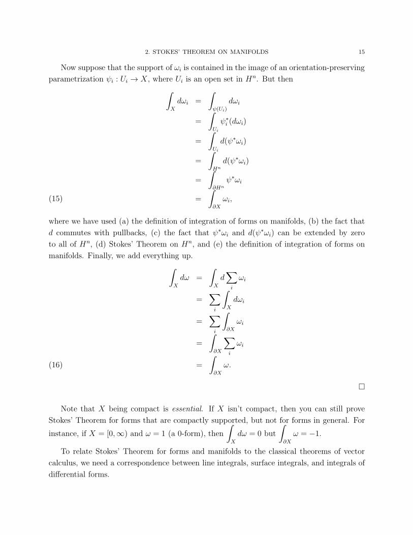
Now suppose that the support of ωi is contained in the image of an orientation-preserving
parametrization ψi : Ui → X , where Ui is an open set in Hn. But then
∫
X
dωi =
∫
ψ(Ui)
dωi
=
∫
Ui
ψ∗
i (dωi)
=
∫
Ui
d(ψ∗ωi)
=
∫
Hn
d(ψ∗ωi)
=
∫
∂Hn
ψ∗ωi
=
∫
∂X
ωi,(15)
where we have used (a) the definition of integration of forms on manifolds, (b) the fact that
d commutes with pullbacks, (c) the fact that ψ∗ωi and d(ψ∗ωi) can be extended by zero
to all of Hn, (d) Stokes’ Theorem on Hn, and (e) the definition of integration of forms on
manifolds. Finally, we add everything up.
∫
X
dω =
∫
X
d∑
i
ωi
=∑
i
∫
X
dωi
=∑
i
∫
∂X
ωi
=
∫
∂X
∑
i
ωi
=
∫
∂X
ω.(16)
Note that X being compact is essential. If X isn’t compact, then you can still prove
Stokes’ Theorem for forms that are compactly supported, but not for forms in general. For
instance, if X = [0,∞) and ω = 1 (a 0-form), then
∫
X
dω = 0 but
∫
∂X
ω = −1.
To relate Stokes’ Theorem for forms and manifolds to the classical theorems of vector
calculus, we need a correspondence between line integrals, surface integrals, and integrals of
differential forms.
16 2. STOKES’ THEOREM
Exercise 1 If γ is an oriented path in R3 and ~v(x) is a vector field, show that
∫
γ
ω1~v is the
line integral
∫
~v ·Tds, where T is the unit tangent to the curve and ds is arclength measure.
(Note that this works for arbitrary smooth paths, and not just for embeddings. It makes
perfectly good sense to integrate around a figure-8.)
Exercise 2 If S is an oriented surface in R3 and ~v is a vector field, show that
∫
S
ω2~v is the
flux of ~v through S.
Exercise 3 Suppose that X is a compact connected oriented 1-manifold-with-boundary in
Rn. (In other words, a path without self-crossings from a to b, where a and b might be
the same point.) Show that Stokes’ Theorem, applied to X , is essentially the Fundamental
Theorem of Calculus.
Exercise 4 Now suppose that X is a bounded domain in R2. Write down Stokes’ Theorem
in this setting and relate it to the classical Green’s Theorem.
Exercise 5 Now suppose that S is an oriented surface in R3 with boundary curve C = ∂S.
Let ~v be a vector field. Apply Stokes Theorem to ω1~v and to S, and express the result in terms
of line integrals and surface integrals. This should give you the classical Stokes’ Theorem.
Exercise 6 On R3, let ω = (x2 + y2)dx ∧ dy + (x + yez)dy ∧ dz + exdx ∧ dz. Compute
∫
S
ω, where S is the upper hemisphere of the unit sphere. The answer depends on which
orientation you pick for S of course. Pick one, and compute! [Hint: Find an appropriate
surface S ′ so that S − S ′ is the boundary of a 3-manifold. Then use Stokes’ Theorem to
relate
∫
S
ω to
∫
S′
ω.]
Exercise 7 On R2 with the origin removed, let α = (xdy − ydx)/(x2 + y2). You previously
showed that dα = 0 (aka “α is closed”). Show that α is not d of any function (“α is not
exact”)
Exercise 8 On R3 with the origin removed, show that β = (xdy ∧ dz − ydx ∧ dz + zdx ∧
dy)/(x2 + y2 + z2)3/2 is closed but not exact.
Exercise 9 Let X be a compact oriented n-manifold (without boundary), let Y be a mani-
fold, and let ω be a closed n-form on Y . Suppose that f0 and f1 are homotopic maps X → Y .
Show that
∫
X
f ∗
0ω =
∫
X
f ∗
1ω.
Exercise 10 Let f : S1 → R2 − 0 be a smooth map whose winding number around the
origin is k. Show that
∫
S1
f ∗α = 2πk, where α is the form of Exercise 7.
CHAPTER 3
Tensors
1. What is a tensor?
Let V be a finite-dimensional vector space.1 It could be Rn, it could be the tangent space
to a manifold at a point, or it could just be an abstract vector space. A k-tensor is a map
T : V × · · · × V → R
(where there are k factors of V ) that is linear in each factor.2 That is, for fixed ~v2, . . . , ~vk,
T (~v1, ~v2, . . . , ~vk−1, ~vk) is a linear function of ~v1, and for fixed ~v1, ~v3, . . . , ~vk, T (~v1, . . . , ~vk) is a
linear function of ~v2, and so on. The space of k-tensors on V is denoted T k(V ∗).
Examples:
• If V = Rn, then the inner product P (~v, ~w) = ~v · ~w is a 2-tensor. For fixed ~v it’s
linear in ~w, and for fixed ~w it’s linear in ~v.
• If V = Rn, D(~v1, . . . , ~vn) = det
(
~v1 · · · ~vn)
is an n-tensor.
• If V = Rn, Three(~v) = “the 3rd entry of ~v” is a 1-tensor.
• A 0-tensor is just a number. It requires no inputs at all to generate an output.
Note that the definition of tensor says nothing about how things behave when you rotate
vectors or permute their order. The inner product P stays the same when you swap the two
vectors, but the determinant D changes sign when you swap two vectors. Both are tensors.
For a 1-tensor like Three, permuting the order of entries doesn’t even make sense!
Let ~b1, . . . ,~bn be a basis for V . Every vector ~v ∈ V can be uniquely expressed as a
linear combination:
~v =∑
i
vi~bi,
where each vi is a number. Let φi(~v) = vi. The map φi is manifestly linear (taking ~bi to 1
and all the other basis vectors to zero), and so is a 1-tensor. In fact, the φi’s form a basis
1Or even an infinite-dimensional vector space, if you apply appropriate regularity conditions.2Strictly speaking, this is what is called a contravariant tensor. There are also covariant tensors and
tensors of mixed type, all of which play a role in differential geometry. But for understanding forms, we onlyneed contravariant tensors.
17
18 3. TENSORS
for the space of 1-tensors. If α is any 1-tensor, then
α(~v) = α(∑
i
vi~bi)
=∑
i
viα(~bi) by linearity
=∑
i
α(~bi)φi(~v) since vi = φi(~v)
= (∑
i
α(~bi)φi)(~v) by linearity, so
α =∑
i
α(~bi)φi.(17)
A bit of terminology: The space of 1-tensors is called the dual space of V and is often
denoted V ∗. The basis φi for V ∗ is called the dual basis of bj. Note that
φi(~bj) = δij :=
1 i = j
0 i 6= j,
and that there is a duality between vectors and 1-tensors (also called co-vectors).
~v =∑
vi~bi where vi = φi(~v)
α =∑
αjφj where αj = α(~bj)
α(~v) =∑
αivi.
It is sometimes convenient to express vectors as columns and co-vectors as rows. The basis
vector ~bi is represented by a column with a 1 in the i-th slot and 0’s everywhere else, while
φj is represented by a row with a 1 in the jth slot and the rest zeroes. Unfortunately,
representing tensors of order greater than 2 visually is difficult, and even 2-tensors aren’t
properly described by matrices. To handle 2-tensors or higher, you really need indices.
If α is a k-tensor and β is an ℓ-tensor, then we can combine them to form a k+ ℓ tensor
that we denote α⊗ β and call the tensor product of α and β:
(α⊗ β)(~v1, . . . , ~vk+ℓ) = α(~v1, . . . , ~vk)β(~vk+1, . . . , ~vk+ℓ).
For instance,
(φi ⊗ φj)(~v, ~w) = φi(~v)φj(~w) = viwj.
Not only are the φi ⊗ φj’s 2-tensors, but they form a basis for the space of 2-tensors. The
proof is a generalization of the description above for 1-tensors, and a specialization of the
following exercise.
Exercise 1: For each ordered k-index I = i1, . . . , ik (where each number can range from
1 to n), let φI = φi1⊗φi2⊗· · ·⊗φik . Show that the φI ’s form a basis for T k(V ∗), which thus
2. ALTERNATING TENSORS 19
has dimension nk. [Hint: If α is a k-tensor, let αI = α(~bi1 , . . . ,~bik). Show that α =
∑
I
αI φI .
This implies that the φI ’s span T k(V ∗). Use a separate argument to show that the φI ’s are
linearly independent.]
Among the k-tensors, there are some that have special properties when their inputs
are permuted. For instance, the inner product is symmetric, with ~v · ~w = ~w · ~v, while
the determinant is anti-symmetric under interchange of any two entries. We can always
decompose a tensor into pieces with distinct symmetry.
For instance, suppose that α is an arbitrary 2-tensor. Define
α+(~v, ~w) =1
2(α(~v, ~w) + α(~w,~v)) ; α−(~v, ~w) =
1
2(α(~v, ~w)− α(~w,~v)) .
Then α+ is symmetric, α− is anti-symmetric, and α = α+ + α−.
2. Alternating Tensors
Our goal is to develop the theory of differential forms. But k-forms are made for integrat-
ing over k-manifolds, and integration means measuring volume. So the k-tensors of interest
should behave qualitatively like the determinant tensor on Rk, which takes k vectors in R
k
and returns the (signed) volume of the parallelpiped that they span. In particular, it should
change sign whenever two arguments are interchanged.
Let Sk denote the group of permutations of (1, . . . , k). A typical element will be denoted
σ = (σ1, . . . , σk). The sign of σ is +1 if σ is an even permutation, i.e. the product of an even
number of transpositions, and −1 if σ is an odd permutation.
We say that a k-tensor α is alternating if, for any σ ∈ Sk and any (ordered) collection
~v1, . . . , ~vk of vectors in V ,
α(~vσ1 , . . . , ~vσk) = sign(σ)α(~v1, . . . , vk).
The space of alternating k-tensors on V is denoted Λk(V ∗). Note that Λ1(V ∗) = T 1(V ∗) = V ∗
and that Λ0(V ∗) = T 0(V ∗) = R.
If α is an arbitrary k-tensor, we define
Alt(α) =1
k!
∑
σ∈Sk
sign(σ)α σ,
or more explicitly
Alt(α)(~v1, . . . , ~vk) =1
k!
∑
σ∈Sk
sign(σ)α(~vσ1 , . . . , ~vσk).
Exercise 2: (in three parts)
(1) Show that Alt(α) ∈ Λk(V ∗).
20 3. TENSORS
(2) Show that Alt, restricted to Λk(V ∗), is the identity. Together with (1), this implies
that Alt is a projection from T k(V ∗) to Λk(V ∗).
(3) Suppose that α is a k-tensor with Alt(α) = 0 and that β is an arbitrary ℓ-tensor.
Show that Alt(α ⊗ β) = 0.
Finally, we can define a product operation on alternating tensors. If α ∈ Λk(V ∗) and
β ∈ Λℓ(V ∗), define
α ∧ β = Ck,ℓAlt(α⊗ β),
where Ck,ℓ is an appropriate constant that depends only on k and ℓ.
Exercise 3: Suppose that α ∈ Λk(V ∗) and β ∈ Λℓ(V ∗), and that Ck,ℓ = Cℓ,k Show that
β ∧ α = (−1)kℓα ∧ β. In other words, wedge products for alternating tensors have the same
symmetry properties as wedge products of forms.
Unfortunately, there are two different conventions for what the constants Ck,ℓ should be!
(1) Most authors, including Spivak, use Ck,ℓ =(k + ℓ)!
k!ℓ!=
(
k + ℓ
k
)
. The advantage of
this convention is that det = φ1 ∧ · · · ∧ φn. The disadvantage of this convention is
that you have to keep track of a bunch of factorials when doing wedge products.
(2) Some authors, including Guillemin and Pollack, use Ck,ℓ = 1. This keeps that alge-
bra of wedge products simple, but has the drawback that φ1∧ · · · ∧φn(~b1, . . . ,~bn) =
1/n! instead of 1. The factorials then reappear in formulas for volume and integra-
tion.
(3) My personal preference is to use Ck,ℓ =
(
k + ℓ
k
)
, and that’s what I’ll do in the
rest of these notes. So be careful when transcribing formulas from Guillemin and
Pollack, since they may differ by some factorials!
Exercise 4: Show that, for both conventions, Ck,ℓCk+ℓ,m = Cℓ,mCk,ℓ+m.
Exercise 5: Suppose that the constants Ck,ℓ are chosen so that Ck,ℓCk+ℓ,m = Cℓ,mCk,ℓ+m,
and suppose that α, β and γ are in Λk(V ∗), Λℓ(V ∗) and Λm(V ∗), respectively. Show that
(α ∧ β) ∧ γ = α ∧ (β ∧ γ).
[If you get stuck, look on page 156 of Guillemin and Pollack].
Exercise 6: Using the convention Ck,ℓ =(k + ℓ)!
k!ℓ!=
(
k + ℓ
k
)
, show that φi1 ∧ · · · ∧ φik =
k!Alt(φi1 ⊗· · ·⊗φik). (If we had picked Ck,ℓ = 1 as in Guillemin and Pollack, we would have
gotten the same formula, only without the factor of k!.)
Let’s take a step back and see what we’ve done.
2. ALTERNATING TENSORS 21
• Starting with a vector space V with basis ~bi, we created a vector space V ∗ =
T 1(V ∗) = Λ1(V ∗) with dual basis φj.
• We defined an associative product ∧ with the property that φj ∧ φi = −φi ∧ φj and
with no other relations.
• Since tensor products of the φj’s span T k(V ∗), wedge products of the φj ’s must
span Λk(V ∗). In other words, Λk(V ∗) is exactly the space that you get by taking
formal products of the φi’s, subject to the anti-symmetry rule.
• That’s exactly what we did with the formal symbols dxj to create differential forms
on Rn. The only difference is that the coefficients of differential forms are functions
rather than real numbers (and that we have derivative and pullback operations on
forms).
• Carrying over our old results from wedges of dxi’s, we conclude that Λk(V ∗) had
dimension
(
n
k
)
=n!
k!(n− k)!and basis φI := φi1 ∧ · · · ∧ φik , where I = i1, . . . , ik
is an arbitrary subset of (1, . . . , n) (with k distinct elements) placed in increasing
order.
• Note the difference between φI = φi1⊗· · ·⊗φik and φI = φi1∧· · ·∧φik . The tensors
φI form a basis for T k(V ∗), while the tensors φI form a basis for Λk(V ∗). They are
related by φI = k!Alt(φI).
Exercise 7: Let V = R3 with the standard basis, and let π : R3 → R
2, π(x, y, z) = (x, y)
be the projection onto the x-y plane. Let α(~v, ~w) be the signed area of the parallelogram
spanned by π(~v) and π(~w) in the x-y plane. Similarly, let β and γ be be the signed areas
of the projections of ~v and ~w in the x-z and y-z planes, respectively. Express α, β and γ
as linear combinations of φi ∧ φj’s. [Hint: If you get stuck, try doing the next two exercises
and then come back to this one.]
Exercise 8: Let V be arbitrary. Show that (φi1 ∧ · · · ∧ φik)(~bj1, . . . ,~bjk) equals +1 if
(j1, . . . , jk) is an even permutation of (i1, . . . , ik), −1 if it is an odd permutation, and 0
if the two lists are not permutations of one another.
Exercise 9: Let α be an arbitrary element of Λk(V ∗). For each subset I = (i1, . . . , ik)
written in increasing order, let αI = α(~bi1 , . . . ,~bik). Show that α =
∑
I
αIφI .
Exercise 10: Now let α1, . . . , αk be an arbitrary ordered list of covectors, and that ~v1, . . . , ~vk
is an arbitrary ordered list of vectors. Show that (α1 ∧ · · · ∧ αk)(~v1, . . . , ~vk) = detA, where
A is the k × k matrix whose i, j entry is αi(~vj).
22 3. TENSORS
3. Pullbacks
Suppose that L : V → W is a linear transformation, and that α ∈ T k(W ∗). We then
define the pullback tensor L∗α by
(19) (L∗α)(~v1, . . . , ~vk) = α(L(~v1), L(~v2), . . . , L(~vk)).
This has some important properties. Pick bases (~b1, . . . ,~bn) and (~d1, . . . , ~dm) for V and
W , respectively, and let φj and ψj be the corresponding dual bases for V ∗ and W ∗. Let
A be the matrix of the linear transformation L relative to the two bases. That is
L(~v)j =∑
j
Ajivi.
Exercise 11: Show that the matrix of L∗ : W ∗ → V ∗, relative to the bases ψj and φj,
is AT . [Hint: to figure out the components of a covector, act on a basis vector]
Exercise 12: If α is a k-tensor, and if I = i1, . . . , ik, show that
(L∗α)I =∑
j1,...,jk
Aj1,i1Aj2,i2 · · ·Ajk,ikα(j1,...,jk).
Exercise 13: Suppose that α is alternating. Show that L∗α is alternating. That is, L∗
restricted to Λk(W ∗) gives a map to Λk(V ∗).
Exercise 14: If α and β are alternating tensors onW , show that L∗(α∧β) = (L∗α)∧(L∗β).
4. Cotangent bundles and forms
We’re finally ready to define forms on manifolds. Let X be a k-manifold. An ℓ-
dimensional vector bundle over X is a manifold E together with a surjection π : E → X
such that
(1) The preimage π−1(p) of any point p ∈ X is an n-dimensional real vector space. This
vector space is called the fiber over p.
(2) For every point p ∈ X there is a neighborhood U and a diffeomorphism φU :
π−1(U) → U × Rn, such that for each x ∈ U , φU restricted to π−1(x) is a linear
isomorphism from π−1(x) to x× Rn (where we think of x× R
n as the vector space
Rn with an additional label x.)
In practice, the isomorphism π−1(U) → U × Rn is usually accomplished by defining a basis
(~v1(x), . . . , ~vn(x)) for the fiber over x, such that each ~vi is a smooth map from U to π−1(U).
Here are some examples of bundles:
• The tangent bundle T (X). In this case n = k. If ψ is a local parametrization around
a point p, then dψ applied to e1, . . . , en give a basis for TpX .
5. RECONCILIATION 23
• The trivial bundle X × V , where V is any n-dimensional vector space. Here we can
pick a constant basis for V .
• The normal bundle of X in Y (where X is a submanifold of Y ).
• The cotangent bundle whose fiber over x is the dual space of Tx(X). This is often
denoted T ∗
x (X), and the entire bundle is denoted T ∗(X). Given a smoothly varying
basis for Tx(X), we can take the dual basis for T ∗
x (X).
• The k-th tensor power of T ∗(X), which we denote T k(T ∗(X)), i.e. the vector bundle
whose fiber over x is T k(T ∗
x (X)).
• The alternating k-tensors in T k(T ∗(X)), which we denote Λk(T ∗(X)).
Some key definitions:
• A section of a vector bundle E → X is a smooth map s : X → E such that π s is
the identity on X . In other words, such that s(x) is an element of the fiber over x
for every x.
• A differential form of degree k is a section of Λk(T ∗(X)). The (infinite-dimensional)
space of k-forms on X is denoted Ωk(X).
• If f : X → R is a function, then dfx : Tx(X) → Tf(x)(R) = R is a covector at X .
Thus every function f defines a 1-form df .
• If f : X → Y is a smooth map of manifolds, then dfx is a linear map Tx(X) →
Tf(x)(Y ), and so induces a pullback map f ∗ : Λk(T ∗
f(x)(Y ))→ Λk(T ∗
x (X)), and hence
a linear map (also denoted f ∗) from Ωk(Y ) to Ωk(X).
Exercise 15: If f : X → Y and g : Y → Z are smooth maps of manifolds, then g f is a
smooth map X → Z. Show that (g f)∗ = f ∗ g∗.
5. Reconciliation
We have developed two different sets of definitions for forms, pullbacks, and the d oper-
ator. Our task in this section is to see how they’re really saying the same thing.
Old definitions:
• A differential form on Rn is a formal sum
∑
αI(x)dxI , where αI(x) is an ordinary
function and dxI is a product dxi1 ∧ · · · ∧ dxik of meaningless symbols that anti-
commute.
• The exterior derivative is dα =∑
I,j
(∂jαI(x))dxj ∧ dxI .
24 3. TENSORS
• If g : Rn → Rm, then the pullback operator g is designed to pull back functions,
commute with d, and respect wedge products: If α =∑
αI(y)dyI, then
g∗(α)(x) =∑
I
αI(g(x))dgi1 ∧ · · · ∧ dgik .
• Forms on n-manifolds are defined via forms on Rn and local coordinates and have
no intrinsic meaning.
New definitions:
• A differential form on Rn is a section of Λk(T ∗(Rn)). Its value at each point x is an
alternating tensor that takes k tangent vectors at that point as inputs and outputs
a number.
• The exterior derivative on functions is defined as the usual derivative map df :
T (X)→ R. We have not yet defined it for higher-order forms.
• If g : X → Y , then the pullback map Ωk(Y )→ Ωk(X) is induced by the derivative
map dg : T (X)→ T (Y ).
• Forms on manifolds do not require a separate definition from forms on Rn, since
tangent spaces, dual spaces, and tensors on tangent spaces are already well-defined.
Our strategy for reconciling these two sets of definitions is:
(1) Show that forms on Rn are the same in both definitions.
(2) Extend the new definition of d to cover all forms, and show that it agrees with the
old definition on Euclidean spaces.
(3) Show that the new definition of pullback, restricted to Euclidean spaces, satisfies
the same axioms as the old definition, and thus gives the same operation on maps
between Euclidean spaces, and in particular for change-of-coordinate maps.
(4) Show that the functional relations that were assumed when we extended the old
definitions to manifolds are already satisfied by the new definitions.
(5) Conclude that the new definitions give a concrete realization of the old definitions.
On Rn, the standard basis for the tangent space is ~e1, . . . , ~en. Since ∂x
j/∂xi = δji , dxj
maps ~ej to 1 and maps all other ~ei’s to zero. Thus the covectors dxx1, . . . , dxx
n (meaning the
derivatives of the functions x1, . . . , xn at the point x) form a basis for T ∗
x (Rn) that is dual to
~e1, . . . , ~en. In other words, φi = dxi!! The meaningless symbols dxi of the old definition
are nothing more (or less) than the dual basis of the new definition. A new-style form is a
linear combination∑
I
αIφI and an old-style form was a linear combination
∑
I
αIdxI , so
the two definitions are exactly the same on Rn. This completes step 1.
5. RECONCILIATION 25
Next we want to extend the (new) definition of d to cover arbitrary forms. We would
like it to satisfy d(α ∧ β) = (dα) ∧ β + (−1)kα ∧ dβ and d2 = 0, and that is enough.
d(dxi) = d2(xi) = 0
d(dxi ∧ dxj) = d(dxi) ∧ dxj − dxi ∧ d(dxj) = 0, and similarly
d(dxI) = 0 by induction on the degree of I.(20)
This then forces us to take
d(∑
I
αIdxI) =
∑
I
(dαI) ∧ dxI + αId(dx
I)
=∑
I
(dαI)dxI
=∑
I,j
(∂jαI)dxj ∧ dxI ,(21)
which is exactly the same formula as before. Note that this construction also works to define
d uniquely on manifolds, as long as we can find functions f i on a neighborhood of a point
p such that the df i’s span T ∗
p (X). But such functions are always available via the local
parametrization. If ψ : U → X is a local parametrization, then we can just pick f i to be the
i-th entry of ψ−1. That is f i = xi ψ−1. This gives a formula for d on X that is equivalent
to “convert to Rn using ψ, compute d in R
n, and then convert back”, which was our old
definition of d on a manifold.
We now check that the definitions of pullback are the same. Let g : Rn → Rm. Under
the new definition, g∗(dyi)(~v) = dyi(dg(~v)), which is the ith entry of dg(~v), where we are
using coordinates yi on Rm. But that is the same as dgi(~v), so g∗(dyi) = dgi. Since the
pullback of a function f is just the composition f g, and since g∗(α∧β) = (g∗(α))∧ (g∗(β))
(see the last exercise in the “pullbacks” section), we must have
g∗(∑
I
αIdyI)(x) =
∑
I
αI(g(x))dgi1 ∧ · · · ∧ dgik ,
exactly as before. This also shows that g∗(dα) = d(g∗α), since that identity is a consequence
of the formula for g∗.
Next we consider forms on manifolds. Let X be an n-manifold, let ψ : U → X be a
parametrization, where U is an open set in Rn. Suppose that a ∈ U , and let p = ψ(a). The
standard bases for Ta(Rn) and T ∗
a (Rn) are ~e1, . . . , ~en and dx
1, . . . , dxn. Let ~bi = dg0(~ei).
The vectors ~bi form a basis for Tp(X). Let φj be the dual basis. But then
ψ∗(φj)(~ei) = φj(dga(~ei))
= φj(~bi)
= δji
26 3. TENSORS
= dxj(~ei), so
ψ∗(φj) = dxj .(22)
Under the old definition, forms on X were abstract objects that corresponded, via pullback,
to forms on U , such that changes of coordinates followed the rules for pullbacks of maps
Rn → R
n. Under the new definition, ψ∗ automatically pulls a basis for T ∗
p (X) to a basis
for T ∗
a (Rn), and this extends to an isomorphism between forms on a neighborhood of p and
forms on a neighborhood of a. Furthermore, if ψ1,2 are two different parametrizations of the
same neighborhood of p, and if ψ1 = ψ2 g12 (so that g12 maps the ψ1 coordinates to the ψ2
coordinates), then we automatically have ψ∗
1 = g∗12 ψ∗
2 , thanks to Exercise 15.
Bottom line: It is perfectly legal to do forms the old way, treating the dx’s as meaningless
symbols that follow certain axioms, and treating forms on manifolds purely via how they
appear in various coordinate systems. However, sections of bundles of alternating tensors on
T (X) give an intrinsic realization of the exact same algebra. The new definitions allow us
to talk about what differential forms actually are, and to develop a cleaner intuition on how
forms behave. In particular, they give a very simple explanation of what integration over
manifolds really means.
CHAPTER 4
Integration
1. The whole is the sum of the parts
Before we go about making sense of integrating forms over manifolds, we need to under-
stand what integrating functions over Rn actually means. When somebody writes∫ 3
0
exdx
or∫
R2
e−(x2+y2)dx dy
or∫
R
f(x)dnx,
what is actually being computed?
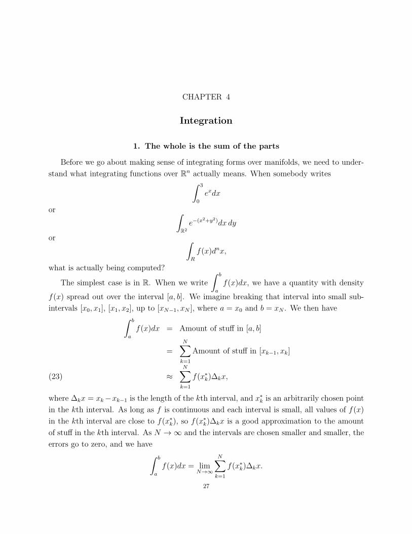
The simplest case is in R. When we write
∫ b
a
f(x)dx, we have a quantity with density
f(x) spread out over the interval [a, b]. We imagine breaking that interval into small sub-
intervals [x0, x1], [x1, x2], up to [xN−1, xN ], where a = x0 and b = xN . We then have∫ b
a
f(x)dx = Amount of stuff in [a, b]
=N∑
k=1
Amount of stuff in [xk−1, xk]
≈
N∑
k=1
f(x∗k)∆kx,(23)
where ∆kx = xk−xk−1 is the length of the kth interval, and x∗k is an arbitrarily chosen point
in the kth interval. As long as f is continuous and each interval is small, all values of f(x)
in the kth interval are close to f(x∗k), so f(x∗
k)∆kx is a good approximation to the amount
of stuff in the kth interval. As N →∞ and the intervals are chosen smaller and smaller, the
errors go to zero, and we have
∫ b
a
f(x)dx = limN→∞
N∑
k=1
f(x∗k)∆kx.
27
28 4. INTEGRATION
Note that I have not required that all of the intervals [xk−1, xk] be the same size! While
that’s convenient, it’s not actually necessary. All we need for convergence is for all of the
sizes to go to zero in the N →∞ limit.
The same idea goes in higher dimensions, when we want to integrate any continuous
bounded function over any bounded region. We break the region into tiny pieces, estimate
the contribution of each piece, and add up the contributions. As the pieces are chosen smaller
and smaller, the errors in our estimates go to zero, and the limit of our sum is our exact
integral.
If we want to integrate an unbounded function, or integrate over an unbounded region,
we break things up into bounded pieces and add up the integrals over the (infinitely many)
pieces. A function is (absolutely) integrable if the pieces add up to a finite sum, no matter
how we slice up the pieces. Calculus books sometimes distinguish between “Type I” improper
integrals like
∫
∞
1
x−3/2dx and “Type II” improper integrals like
∫ 1
0
y−1/2dy, but they are
really the same. Just apply the change of variables y = 1/x:∫
∞
1
x−3/2dx =∞∑
k=1
∫ k+1
k
x−3/2dx
=∞∑
k=1
∫ 1/k
1/(k+1)
y−1/2dy
=
∫ 1
0
y−1/2dy.(24)
When doing such a change of variables, the width of the intervals can change drastically.
∆y is not ∆x, and x-intervals of size 1 turn into y-intervals of size1
k(k + 1). Likewise, the
integrand is not the same. However, the contribution of the interval, whether written as
x−3/2∆x or y−1/2∆y, is the same (at least in the limit of small intervals).
In other words, we need to stop thinking about f(x) and dx separately, and think instead
of the combination f(x)dx, which is a machine for extracting the contribution of each small
interval.
But that’s exactly what the differential form f(x)dx is for! In one dimension, the covector
dx just gives the value of a vector in R1. If we evaluate f(x)dx at a sample point x∗k and
apply it to the vector xk − xk−1, we get
f(x)dx(~xk − ~xk−1) = f(x∗k)∆kx.
2. Integrals in 2 or More Dimensions
Likewise, let’s try to interpret the integral of f(x, y)dxdy over a rectangle R = [a, b]×[c, d]
in R2. The usual approach is to break the interval [a, b] into N pieces and the interval
2. INTEGRALS IN 2 OR MORE DIMENSIONS 29
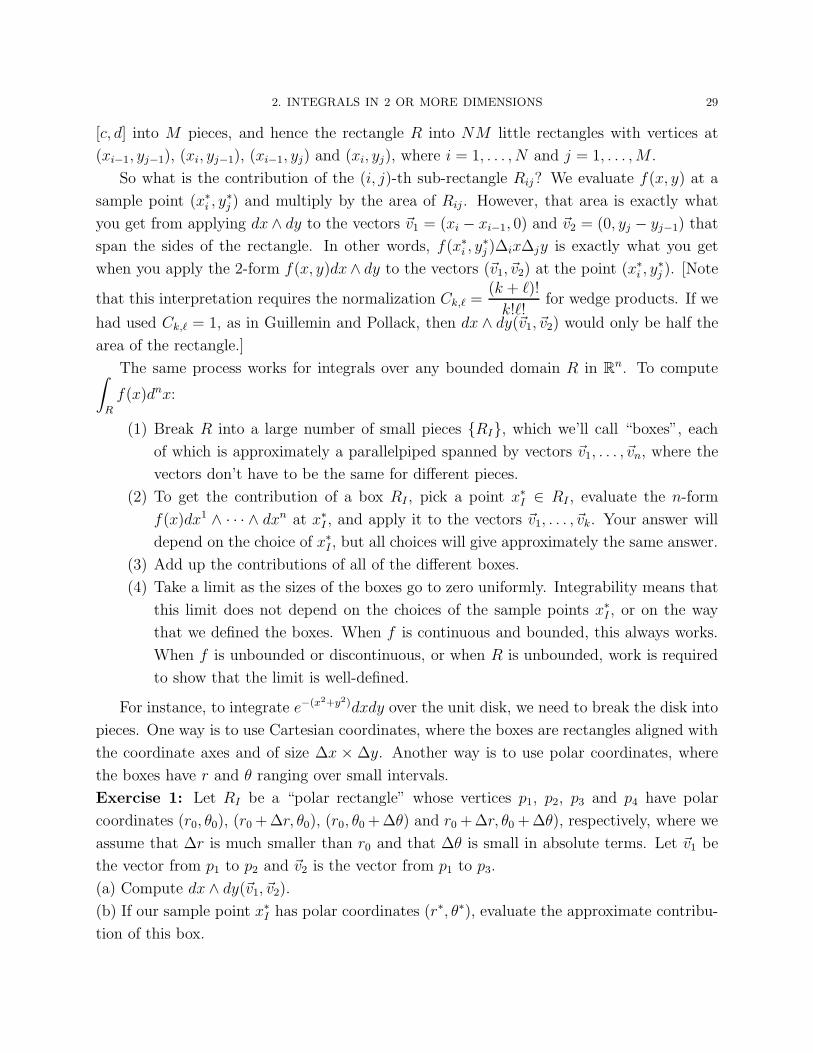
[c, d] into M pieces, and hence the rectangle R into NM little rectangles with vertices at
(xi−1, yj−1), (xi, yj−1), (xi−1, yj) and (xi, yj), where i = 1, . . . , N and j = 1, . . . ,M .
So what is the contribution of the (i, j)-th sub-rectangle Rij? We evaluate f(x, y) at a
sample point (x∗i , y∗
j ) and multiply by the area of Rij . However, that area is exactly what
you get from applying dx ∧ dy to the vectors ~v1 = (xi − xi−1, 0) and ~v2 = (0, yj − yj−1) that
span the sides of the rectangle. In other words, f(x∗i , y∗
j )∆ix∆jy is exactly what you get
when you apply the 2-form f(x, y)dx∧ dy to the vectors (~v1, ~v2) at the point (x∗i , y∗
j ). [Note
that this interpretation requires the normalization Ck,ℓ =(k + ℓ)!
k!ℓ!for wedge products. If we
had used Ck,ℓ = 1, as in Guillemin and Pollack, then dx ∧ dy(~v1, ~v2) would only be half the
area of the rectangle.]
The same process works for integrals over any bounded domain R in Rn. To compute
∫
R
f(x)dnx:
(1) Break R into a large number of small pieces RI, which we’ll call “boxes”, each
of which is approximately a parallelpiped spanned by vectors ~v1, . . . , ~vn, where the
vectors don’t have to be the same for different pieces.
(2) To get the contribution of a box RI , pick a point x∗I ∈ RI , evaluate the n-form
f(x)dx1 ∧ · · · ∧ dxn at x∗I , and apply it to the vectors ~v1, . . . , ~vk. Your answer will
depend on the choice of x∗I , but all choices will give approximately the same answer.
(3) Add up the contributions of all of the different boxes.
(4) Take a limit as the sizes of the boxes go to zero uniformly. Integrability means that
this limit does not depend on the choices of the sample points x∗I , or on the way
that we defined the boxes. When f is continuous and bounded, this always works.
When f is unbounded or discontinuous, or when R is unbounded, work is required
to show that the limit is well-defined.
For instance, to integrate e−(x2+y2)dxdy over the unit disk, we need to break the disk into
pieces. One way is to use Cartesian coordinates, where the boxes are rectangles aligned with
the coordinate axes and of size ∆x × ∆y. Another way is to use polar coordinates, where
the boxes have r and θ ranging over small intervals.
Exercise 1: Let RI be a “polar rectangle” whose vertices p1, p2, p3 and p4 have polar
coordinates (r0, θ0), (r0+∆r, θ0), (r0, θ0+∆θ) and r0 +∆r, θ0 +∆θ), respectively, where we
assume that ∆r is much smaller than r0 and that ∆θ is small in absolute terms. Let ~v1 be
the vector from p1 to p2 and ~v2 is the vector from p1 to p3.
(a) Compute dx ∧ dy(~v1, ~v2).
(b) If our sample point x∗I has polar coordinates (r∗, θ∗), evaluate the approximate contribu-
tion of this box.
30 4. INTEGRATION
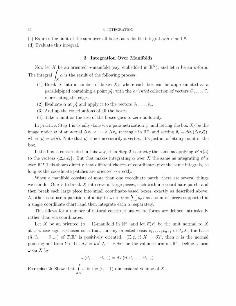
(c) Express the limit of the sum over all boxes as a double integral over r and θ.
(d) Evaluate this integral.
3. Integration Over Manifolds
Now let X be an oriented n-manifold (say, embedded in RN), and let α be an n-form.
The integral
∫
X
α is the result of the following process.
(1) Break X into a number of boxes XI , where each box can be approximated as a
parallelpiped containing a point p∗I , with the oriented collection of vectors ~v1, . . . , ~vn
representing the edges.
(2) Evaluate α at p∗I and apply it to the vectors ~v1, . . . , ~vn.
(3) Add up the contributions of all the boxes.
(4) Take a limit as the size of the boxes goes to zero uniformly.
In practice, Step 1 is usually done via a parametrization ψ, and letting the box XI be the
image under ψ of an actual ∆x1 × · · · ×∆xn rectangle in Rn, and setting ~vi = dψa(∆xi~ei),
where p∗I = ψ(a). Note that p∗I is not necessarily a vertex. It’s just an arbitrary point in the
box.
If the box is constructed in this way, then Step 2 is exactly the same as applying ψ∗α(a)
to the vectors ∆xi~ei. But that makes integrating α over X the same as integrating ψ∗α
over Rn! This shows directly that different choices of coordinates give the same integrals, as
long as the coordinate patches are oriented correctly.
When a manifold consists of more than one coordinate patch, there are several things
we can do. One is to break X into several large pieces, each within a coordinate patch, and
then break each large piece into small coordinate-based boxes, exactly as described above.
Another is to use a partition of unity to write α =∑
ρiα as a sum of pieces supported in
a single coordinate chart, and then integrate each αi separately.
This allows for a number of natural constructions where forms are defined intrinsically
rather than via coordinates.
Let X be an oriented (n − 1)-manifold in Rn, and let ~n(x) be the unit normal to X
at x whose sign is chosen such that, for any oriented basis ~v1, . . . , ~vn−1 of TxX , the basis
(~n,~v1, . . . , ~vn−1) of TxRn is positively oriented. (E.g, if X = ∂Y , then n is the normal
pointing out from Y ). Let dV = dx1 ∧ · · · ∧ dxn be the volume form on Rn. Define a form
ω on X by
ω(~v1, . . . , ~vn−1) = dV (~n,~v1, . . . , ~vn−1).
Exercise 2: Show that
∫
X
ω is the (n− 1)-dimensional volume of X .
3. INTEGRATION OVER MANIFOLDS 31
More generally, let α be any k-form on a manifold X , and let ~w(x) be any vector field.
We define a new (k − 1)-form iwα by
(iwα)(~v1, . . . , ~vk−1) = α(~w,~v1, . . . , ~vk−1).
Exercise 3: Let S be a surface in R3 and let ~v(x) be a vector field. Show directly that
∫
S
iv(dx∧dy∧dz) is the flux of ~v through S. That is, show that iv(dx∧dy∧dz) applied to a
pair of (small) vectors gives (approximately) the flux of ~v through a parallelogram spanned
by those vectors.
Exercise 4: In R3 we have already seen iv(dx ∧ dy ∧ dz). What did we call it?
Exercise 5: Let ~v be any vector field in Rn. Compute d(iv(dx
1 ∧ · · · ∧ dxn)).
Exercise 6: Let α =∑
αI(x)dxI be a k-form on R
n and let ~v(x) = ~ei, the i-th standard
basis vector for Rn. Compute d(ivα)+ iv(dα). Generalize to the case where ~v is an arbitrary
constant vector field.
When ~v is not constant, the expression d(ivα)+ iv(dα) is more complicated, and depends
both on derivatives of v and derivatives of αI , as we saw in the last two exercises. This
quantity is called the Lie derivative of α with respect to ~v.
It is certainly possible to feed more than one vector field to a k-form, thereby reducing
its degree by more than 1. It immediately follows that iviw = −iwiv as a map Ωk(X) →
Ωk−2(X).

CHAPTER 5
de Rham Cohomology
1. Closed and exact forms
Let X be a n-manifold (not necessarily oriented), and let α be a k-form on X . We say
that α is closed if dα = 0 and say that α is exact if α = dβ for some (k − 1)-form β. (When
k = 0, the 0 form is also considered exact.) Note that
• Every exact form is closed, since d(dβ) = d2β = 0.
• A 0-form is closed if and only if it is locally constant, i.e. constant on each connected
component of X .
• Every n-form is closed, since then dα would be an (n+1)-form on an n-dimensional
manifold, and there are no nonzero (n + 1)-forms.
Since the exact k-forms are a subspace of the closed k-forms, we can defined the quotient
space
HkdR(X) =
Closed k-forms on X
Exact k-forms on X.
This quotient space is called the kth de Rham cohomology of X . Since this is the only kind of
cohomology we’re going to discuss in these notes, I’ll henceforth omit the prefix “de Rham”
and the subscript dR. If α is a closed form, we write [α] to denote the class of α in Hk, and
say that the form α represents the cohomology class [α].
The wedge product of forms extends to a product operationHk(X)×Hℓ(X)→ Hk+ℓ(X).
If α and β are closed, then
d(α ∧ β) = (dα) ∧ β + (−1)kα ∧ dβ
= 0 ∧ β ± α ∧ 0 = 0,
so α ∧ β is closed. Thus α ∧ β represents a class in Hk+ℓ, and we define
[α] ∧ [β] = [α ∧ β].
We must check that this is well-defined. I’m going to spell this out in gory detail as an
example of computations to come.
Suppose that [α′] = [α] and [β ′] = [β]. We must show that [α′ ∧ β ′] = [α ∧ β]. However
[α′] = [α] means that α′ and α differ by an exact form, and similarly for β ′ and β:
α′ = α + dµ
33
34 5. DE RHAM COHOMOLOGY
β ′ = β + dν
But then
α′ ∧ β ′ = (α+ dµ) ∧ (β + dν)
= α ∧ β + (dµ) ∧ β + α ∧ dν + dµ ∧ dν
= α ∧ β + d(µ ∧ β) + (−1)kd(α ∧ ν) + d(µ ∧ dν)
= α ∧ β + exact forms,
where we have used the fact that d(µ ∧ β) = dµ ∧ β + (−1)k−1µ ∧ dβ = dµ ∧ β, and similar
expansions for the other terms. That is,
(Exact) ∧ (Closed) = (Exact)
(Closed) ∧ (Exact) = (Exact)
(Exact) ∧ (Exact) = (Exact)
Thus α′ ∧ β ′ and α ∧ β represent the same class in cohomology. Since β ∧ α = (−1)kℓα ∧ β,
it also follows immediately that [β] ∧ [α] = (−1)kℓ[α] ∧ [β].
We close this section with a few examples.
• If X is a point, then H0(X) = Ω0(X) = R, and Hk(X) = 0 for all k 6= 0, since there
are no nonzero forms in dimension greater than 1.
• If X = R, then H0(X) = R, since the closed 0-forms are the constant functions,
of which only the 0 function is exact. All 1-forms are both closed and exact. If
α = α(x)dx is a 1-form, then α = df , where f(x) =
∫ x
0
α(s)ds is the indefinite
integral of α(x).
• If X is any connected manifold, then H0(X) = R.
• IfX = S1 (say, embedded in R2), thenH1(X) = R, and the isomorphism is obtained
by integration: [α] →
∫
S1
α. If the form α is exact, then
∫
S1
α = 0. Conversely, if∫
S1
α = 0, then f(x) =
∫ x
a
α (for an arbitrary fixed starting point a) is well-defined
and α = df .
2. Pullbacks in Cohomology
Suppose that f : X → Y and that α is a closed form on Y , representing a class in Hk(Y ).
Then f ∗α is also closed, since
d(f ∗α) = f ∗(dα) = f ∗(0) = 0,
3. INTEGRATION OVER A FIBER AND THE POINCARE LEMMA 35
so f ∗α represents a class in Hk(X). If α′ also represents [α] ∈ Hk(Y ), then we must have
α′ = α + dµ, so
f ∗(α′) = f ∗α + f ∗(dµ) = f ∗α + d(f ∗µ)
represents the same class in Hk(X) as f ∗α does. We can therefore define a map
f ♯ : Hk(Y )→ Hk(X), f ♯[α] = [f ∗α].
We are using notation to distinguish between the pullback map f ∗ on forms and the pullback
map f ♯ on cohomology. Guillemin and Pollack also follow this convention. However, most
authors use f ∗ to denote both maps, hoping that it is clear from context whether we are
talking about forms or about the classes they represent. (Still others use f ♯ for the map on
forms and f ∗ for the map on cohomology. Go figure.)
Note that f ♯ is a contravariant functor, which is a fancy way of saying that it reverses
the direction of arrows. If f : X → Y , then f ♯ : Hk(X) ← Hk(Y ). If f : X → Y and
g : Y → Z, then g♯ : Hk(Z)→ Hk(Y ) and f ♯ : Hk(Y )→ Hk(X). Since (g f)∗ = f ∗ g∗, it
follows that (g f)♯ = f ♯ g♯.
We will have more to say about pullbacks in cohomology after we have established some
more machinery.
3. Integration over a fiber and the Poincare Lemma
Theorem 3.1 (Integration over a fiber). Let X be any manifold. Let the zero section
s0 : X → R × X be given by s0(x) = (0, x), and let the projection π : R × X → X be
given by π(t, x) = x. Then s♯0 : Hk(R × X) → Hk(X) and π♯ : Hk(X) → Hk(R × X) are
isomorphisms and are inverses of each other.
Proof. Since π s0 is the identity on X , s♯0 π♯ is the identity on Hk(X). We must
show that π♯ s♯0 is the identity on Hk(R × X). We do this by constructing a map P :
Ωk(R × X) → Ωk−1(R × X), called a homotopy operator, such that for any k form α on
R×X ,
(1− π∗ s∗) = d(P (α)) + P (dα).
If α is closed, this implies that α and π∗(s∗0α) differ by the exact form d(P (α)) and so
represent the same class in cohomology, and hence that π♯ s♯0[α] = [α]. Since this is true
for all α, π♯ s♯0 is the identity.
Every k-form on Y can be uniquely written as a product
α(t, x) = dt ∧ β(t, x) + γ(t, x),
36 5. DE RHAM COHOMOLOGY
where β and γ have no dt factors. The (k − 1)-form β can be written as a sum:
β(t, x) =∑
J
βJ(t, x)dxJ ,
where βJ(t, x) is an ordinary function, and we likewise write
γ(t, x) =∑
I
γI(t, x)dxI .
We define
P (α)(t, x) =∑
J
(
∫ t
0
βJ(s, x)ds)dxJ .
P (α) is called the integral along the fiber of α. Note that s∗0α, evaluated at x, is∑
I
γ(0, x)dxI ,
and that
(1− π∗s∗0)α(t, x) = dt ∧ β(t, x) +∑
I
(γ(t, x)− γ(t, 0))dxI .
Now we compute dP (α) and P (dα). Since
dα(t, x) = −dt ∧∑
j,J
(∂jβJ(t, x))dxj ∧ dxJ +
∑
I
∂tγI(t, x)dt ∧ dxI +
∑
I,j
∂jγI(t, x)dxj ∧ dxI ,
where j runs over the coordinates of X , we have
P (dα)(t, x) = −∑
j,J
∫ t
0
(
∂jβJ(s, x)ds)
dxj ∧ dxJ +∑
I
(
γI(t, x)− γI(0, x))
dxI ,
where we have used
∫ t
0
∂sγI(s, x)ds = γI(t, x)− γI(0, x). Meanwhile,
d(P (α)) =∑
j,J
(∫ t
0
∂jβJ(s, x)ds
)
dxj ∧ dxJ +∑
J
βJ(t, x)dt ∧ dxJ ,
so
(dP + Pd)α(t, x) =∑
I
(
γI(t, x)− γI(0, x))
dxI + dt ∧ β(t, x) = (1− π∗s∗0)α(t, x).
Exercise 1: In this proof, the operator P was defined relative to local coordinates on X .
Show that this is in fact well-defined. That is, if we have two parametrizations ψ and φ, and
we compute P (α) using the φ coordinates and then convert to the ψ coordinates, we get the
same result as if we computed P (α) directly using the ψ coordinates.
An immediate corollary of this theorem is that Hk(Rn) = Hk(Rn−1) = · · · = Hk(R0). In
particular,
3. INTEGRATION OVER A FIBER AND THE POINCARE LEMMA 37
Theorem 3.2 (Poincare Lemma). On Rn, or on any manifold diffeomorphic to R
n, every
closed form of degree 1 or higher is exact.
Exercise 2: Show that a vector field ~v on R3 is the gradient of a function if and only if
∇× ~v = 0 everywhere.
Exercise 3: Show that a vector field ~v on R3 can be written as a curl (i.e., ~v = ∇× ~w) if
and only if ∇ · ~v = 0.
Exercise 4: Now consider the 3-dimensional torus X = R3/Z3. Construct a vector field
~v(x) whose curl is zero that is not a gradient (where we use the local isomorphism with R3
to define the curl and gradient). Construct a vector field ~w(x) whose divergence is zero that
is not a curl.
In the integration-along-a-fiber theorem, we showed that s♯0 was the inverse of π♯. How-
ever, we could have used the 1-section s1(x) = (1, x) instead of the 0-section and obtained
the same result. (Just replace 0 with 1 everwhere that refers to a value of t). Thus
s♯1 = (π♯)−1 = s♯0.
This has important consequences for homotopies.
Theorem 3.3. Homotopic maps induce the same map in cohomology. That is, if X and
Y are manifolds and f0,1 : X → Y are smooth homotopic maps, then f ♯1 = f ♯0.
Proof. If f0 and f1 are homotopic, then we can find a smooth map F : R × X → Y
such that F (t, x) = f0(x) for t ≤ 0 and F (t, x) = f1(x) for t ≥ 1. But then f1 = F s1 and
f0 = F s0. Thus
f ♯1 = s♯1 F♯ = s♯0 F
♯ = (F s0)♯ = f ♯0.
Exercise 5: Recall that if A is a submanifold of X , then a retraction r : X → A (sometimes
just called a retract) is a smooth map such that r(a) = a for all a ∈ A. If such a map
exists, we say that A is a retract of X . Suppose that r : X → A is such a retraction,
and that iA be the inclusion of A in X . Show that r♯ : Hk(A) → Hk(X) is surjective and
i♯A : Hk(X)→ Hk(A) is injective in every degree k. [We will soon see that Hk(Sk) = R. This
exercise, combined with the Poincare Lemma, will then provide another proof that there are
no retractions from the unit ball in Rn to the unit sphere.]
Exercise 6: Recall that a deformation retraction is a retraction r : X → A such that iA r
is homotopic to the identity on X , in which case we say that A is a deformation retract of X .
Suppose that A is a deformation retract of X . Show that Hk(X) and Hk(A) are isomorphic.
[This provides another proof of the Poincare Lemma, insofar as Rn deformation retracts to
a point.]
38 5. DE RHAM COHOMOLOGY
4. Mayer-Vietoris Sequences 1: Statement
Suppose that a manifold X can be written as the union of two open submanifolds, U
and V . The Mayer-Vietoris Sequence is a technique for computing the cohomology of X
from the cohomologies of U , V and U ∩ V . This has direct practical importance, in that it
allows us to compute things like Hk(Sn) and many other simple examples. It also allows us
to prove many properties of compact manifolds by induction on the number of open sets in
a “good cover” (defined below). Among the things that can be proved with this technique
(of which we will only prove a subset) are:
(1) Hk(Sn) = R if k = 0 or k = n and is trivial otherwise.
(2) If X is compact, then Hk(X) is finite-dimensional. This is hardly obvious, since
Hk(X) is the quotient of the infinite-dimensional vector space of closed k-forms by
another infinite-dimensional space of exact k-forms. But as long as X is compact,
the quotient is finite-dimensional.
(3) If X is a compact, oriented n-manifold, then Hn(X) = R.
(4) If X is a compact, oriented n-manifold, then Hk(X) is isomorphic to Hn−k(X).
(More precisely to the dual of Hn−k(X), but every finite-dimensional vector space
is isomorphic to its own dual.) This is called Poincare duality.
(5) If X is any compact manifold, orientable or not, then Hk(X) is isomorphic to
Hom(Hk(X),R), where Hk(X) is the k-th homology group of X .
(6) A formula for Hk(X × Y ) in terms of the cohomologies of X and Y .
Suppose we have a sequence
V 1 L1−→ V 2 L2−→ V 3 L3−→ · · ·
where each V i is a vector space and each Li : Vi → V i+1 is a linear transformation. We say
that this sequence is exact if the kernel of each Li equals the image of the previous Li−1. In
particular,
0 −→ VL−→ W −→ 0
is exact if and only if L is an isomorphism, since the kernel of L has to equal the image of
0, and the image of L has to equal the kernel of the 0 map on W .
Exercise 7: A short exact sequence involves three spaces and two maps:
0→ Ui−→ V
j−→ W → 0
Show that if this sequence is exact, there must be an isomorphism h : V → U ⊕W , with
h i(u) = (u, 0) and j h−1(u, w) = w.
Exact sequences can be defined for homeomorphisms between arbitrary Abelian groups,
and not just vector spaces, but are much simpler when applied to vector spaces. In particular,
5. PROOF OF MAYER-VIETORIS 39
the analogue of the previous exercise is false for groups. (E.g. one can define a short exact
sequence 0→ Z2 → Z4 → Z2 → 0 even though Z4 is not isomorphic to Z2 × Z2.)
Suppose that X = U ∪ V , where U and V are open submanifolds of X . There are
natural inclusion maps iU and iV of U and V into X , and these induce maps i∗U and i∗V from
Ωk(X) to Ωk(U) and Ωk(V ). Note that i∗U(α) is just the restriction of α to U , while i∗V (α)
is the restriction of α to V . Likewise, there are inclusions ρU and ρV of U ∩ V in U and V ,
respectively, and associated restrictions ρ∗U and ρ∗V from Ωk(U) and Ωk(V ) to Ωk(U ∩ V ).
Together, these form a sequence:
(25) 0→ Ωk(X)ik−→ Ωk(U)⊕ Ωk(V )
jk−→ Ωk(U ∩ V )→ 0,
where the maps are defined as follows. If α ∈ Ωk(X), β ∈ Ωk(U) and γ ∈ Ωk(V ), then
ik(α) = (i∗Uα, i∗
V α)
jk(β, γ) = r∗Uβ − r∗
V γ.
Note that d(ik(α)) = ik+1(dα) and that d(jk(β, γ)) = jk+1(dβ, dγ). That is, the diagram
0 −−−→ Ωk(X)ik−−−→ Ωk(U)⊕ Ωk(V )
jk−−−→ Ωk(U ∪ V ) −−−→ 0
y
dk
y
dk
y
dk
0 −−−→ Ωk+1(X)ik+1
−−−→ Ωk+1(U)⊕ Ωk+1(V )jk+1
−−−→ Ωk+1(U ∪ V ) −−−→ 0
commutes. Thus ik and jk send closed forms to closed forms and exact forms to exact forms,
and induce maps
i♯k : Hk(X)→ Hk(U)⊕Hk(V ); j♯k : H
k(U)⊕Hk(V )→ Hk(U ∩ V ).
Theorem 4.1 (Mayer-Vietoris). There exists a map d♯k : Hk(U ∩ V ) → Hk+1(X) such
that the sequence
· · ·Hk(X)i♯k−→ Hk(U)⊕Hk(V )
j♯k−→ Hk(U ∩ V )
d♯k−→ Hk+1(X)
i♯k+1
−−→ Hk+1(U)⊕Hk+1(V )→ · · ·
is exact.
The proof is a long slog, and warrants a section of its own. Then we will develop the
uses of Mayer-Vietoris sequences.
5. Proof of Mayer-Vietoris
The proof has several big steps.
(1) We show that the sequence (25) of forms is actually exact.
(2) Using that exactness, and the fact that i and j commute with d, we then construct
the map d♯k.
40 5. DE RHAM COHOMOLOGY
(3) Having constructed the maps, we show exactness at Hk(U)⊕Hk(V ), i.e., that the
image of i♯k equals the kernel of j♯k.
(4) We show exactness at Hk(U ∩ V ), i.e., that the image of j♯k equals the kernel of d♯k.
(5) We show exactness at Hk+1(X), i.e. that the kernel of i♯k+1 equals the image of d♯k.
(6) Every step but the first is formal, and applies just as well to any short exact sequence
of (co)chain complexes. This construction in homological algebra is called the snake
lemma, and may be familiar to some of you from algebraic topology. If so, you can
skip ahead after step 2. If not, don’t worry. We’ll cover everything from scratch.
Step 1: Showing that
0→ Ωk(X)ik−→ Ωk(U)⊕ Ωk(V )
jk−→ Ωk(U ∩ V )→ 0
amounts to showing that ik is injective, that Im(ik) = Ker(jk), and that jk is surjective.
The first two are easy. The subtlety is in showing that jk is surjective.
Recall that i∗U , i∗
V , r∗
U and r∗V are all restriction maps. If α ∈ Ωk(X) and ik(α) = 0, then
the restriction of α to U is zero, as is the restriction to V . But then α itself is the zero form
on X . This shows that ik is injective.
Likewise, for any α ∈ Ωk(X), i∗U (α) and i∗
V (α) agree on U ∩ V , so r∗U i∗
U(α) = r∗V i∗
V (α), so
jk(ik(α)) = 0. Conversely, if jk(β, γ) = 0, then r∗U(β) = r∗V (γ), so we can stitch β and γ into
a form α on X that equals β on U and equals γ on V (and equals both of them on U ∩ V ),
so (β, γ) ∈ Im(ik).
Now suppose that µ ∈ Ωk(U ∩ V ) and that ρU , ρV is a partition of unity of X relative
to the open cover U, V . Since the function ρU is zero outside of U , the form ρUµ can be
extended to a smooth form on V by declaring that ρUµ = 0 on V − U . Note that ρUµ is
not a form on U , since µ is not defined on the entire support of ρU . Rather, ρUµ is a form
on V , since µ is defined at all points of V where ρU 6= 0. Likewise, ρV µ is a form on U . On
U ∩ V , we have µ = ρV µ− (−ρUµ). This means that µ = jk(ρV µ,−ρUµ).
The remaining steps are best described in the language of homological algebra. A cochain
complex A is a sequence of vectors spaces1 A0, A1, A2, . . . together with maps dk : Ak →
Ak+1 such that dk dk−1 = 0. We also define A−1 = A−2 = · · · to be 0-dimensional vector
spaces (“0”) and d−1 = d−2 = · · · to be the zero map. The k-th cohomology of the complex
is
Hk(A) =kernel of dkimage of dk−1
.
1For (co)homology theories with integer coefficients one usually considers sequences of Abelian groups.For de Rham theory, vector spaces will do.
5. PROOF OF MAYER-VIETORIS 41
A cochain map i : A→ B between complexes A and B is a family of maps ik : Ak → Bk
such that dk(ik(α)) = ik+1(dkα) for all k and all α ∈ Ak, i.e., such that the diagram
Akik−−−→ Bk
y
dAk
y
dBk
Ak+1 ik+1
−−−→ Bk+1
commutes for all k, where we have labeled the two differential maps dAk and dBk to emphasize
that they are defined on different spaces.
Exercise 8: Show that a cochain map i : A→ B induces maps in cohomology
i♯k : Hk(A)→ Hk(B); [α] 7→ [ikα].
If A, B and C are cochain complexes and i : A → B and j : B → C are cochain maps,
then the sequence
0→ Ai−→ B
j−→ C → 0
is said to be a short exact sequence of cochain complexes if, for each k,
0→ Akik−→ Bk jk−→ Ck → 0
is a short exact sequence of vector spaces.
So far, we have constructed a short exact sequence of cochain complexes with Ak =
Ωk(X), Bk = Ωk(U) ⊕ Ωk(V ), and Ck = Ωk(U ∩ V ). The theorem on Mayer-Vietoris
sequences is then a special case of
Theorem 5.1 (Snake Lemma). Let 0 → Ai−→ B
j−→ C → 0 be a short exact sequence
of cochain complexes. Then there is a family of maps d♯k : Hk(C)→ Hk+1(A) such that the
sequence
· · · → Hk(A)i♯k−→ Hk(B)
j♯k−→ Hk(C)d♯k−→ Hk+1(A)
i♯k+1
−−→ Hk+1(B)→ · · ·
is exact.
We will use the letters α, β, γ, with appropriate subscripts and other markers, to denote
elements of A, B and C, respectively. For simplicity, we will write “d” for dAk , dBk , d
Ck , d
Ak+1,
etc. Our first task is to define d♯k[γk], where [γk] is a class in Hk(C).
Since jk is surjective, we can find βk ∈ Bk such that γk = jk(βk). Now,
jk+1(dβk) = d(jk(βk)) = d(γk) = 0,
since γk was closed. Since dβk is in the kernel of jk+1, it must be in the image of ik+1. Let
αk+1 be such that ik+1(αk+1) = dβk. Furthermore, αk+1 is unique, since ik+1 is injective. We
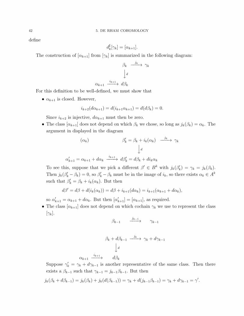
42 5. DE RHAM COHOMOLOGY
define
d♯k[γk] = [αk+1].
The construction of [αk+1] from [γk] is summarized in the following diagram:
βkjk−−−→ γk
yd
αk+1ik+1
−−−→ dβk
For this definition to be well-defined, we must show that
• αk+1 is closed. However,
ik+2(dαk+1) = d(ik+1αk+1) = d(dβk) = 0.
Since ik+2 is injective, dαk+1 must then be zero.
• The class [αk+1] does not depend on which βk we chose, so long as jk(βk) = αk. The
argument in displayed in the diagram
(αk) β ′
k = βk + ik(αk)jk−−−→ γk
yd
α′
k+1 = αk+1 + dαkik+1
−−−→ dβ ′
k = dβk + dikαk
To see this, suppose that we pick a different β ′ ∈ Bk with jk(β′
k) = γk = jk(βk).
Then jk(β′
k−βk) = 0, so β ′
k−βk must be in the image of ik, so there exists αk ∈ Ak
such that β ′
k = βk + ik(αk). But then
dβ ′ = dβ + d(ik(αk)) = dβ + ik+1(dαk) = ik+1(αk+1 + dαk),
so α′
k+1 = αk+1 + dαk. But then [α′
k+1] = [αk+1], as required.
• The class [αk+1] does not depend on which cochain γk we use to represent the class
[γk].
βk−1jk−1
−−−→ γk−1
βk + dβk−1jk−−−→ γk + dγk−1
yd
αk+1ik+1
−−−→ dβkSuppose γ′k = γk + dγk−1 is another representative of the same class. Then there
exists a βk−1 such that γk−1 = jk−1βk−1. But then
jk(βk + dβk−1) = jk(βk) + jk(d(βk−1)) = γk + d(jk−1βk−1) = γk + dγk−1 = γ′.
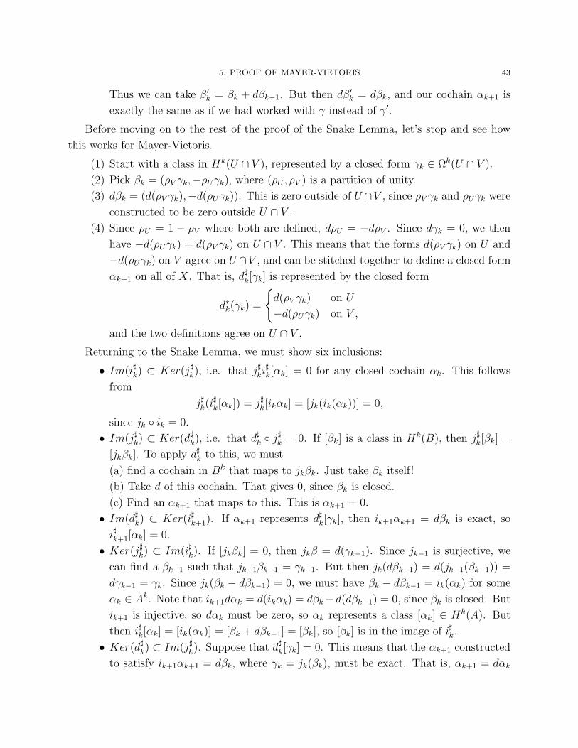
5. PROOF OF MAYER-VIETORIS 43
Thus we can take β ′
k = βk + dβk−1. But then dβ ′
k = dβk, and our cochain αk+1 is
exactly the same as if we had worked with γ instead of γ′.
Before moving on to the rest of the proof of the Snake Lemma, let’s stop and see how
this works for Mayer-Vietoris.
(1) Start with a class in Hk(U ∩ V ), represented by a closed form γk ∈ Ωk(U ∩ V ).
(2) Pick βk = (ρV γk,−ρUγk), where (ρU , ρV ) is a partition of unity.
(3) dβk = (d(ρV γk),−d(ρUγk)). This is zero outside of U ∩V , since ρV γk and ρUγk were
constructed to be zero outside U ∩ V .
(4) Since ρU = 1 − ρV where both are defined, dρU = −dρV . Since dγk = 0, we then
have −d(ρUγk) = d(ρV γk) on U ∩ V . This means that the forms d(ρV γk) on U and
−d(ρUγk) on V agree on U ∩V , and can be stitched together to define a closed form
αk+1 on all of X . That is, d♯k[γk] is represented by the closed form
d∗k(γk) =
d(ρV γk) on U
−d(ρUγk) on V ,
and the two definitions agree on U ∩ V .
Returning to the Snake Lemma, we must show six inclusions:
• Im(i♯k) ⊂ Ker(j♯k), i.e. that j♯ki♯k[αk] = 0 for any closed cochain αk. This follows
from
j♯k(i♯k[αk]) = j♯k[ikαk] = [jk(ik(αk))] = 0,
since jk ik = 0.
• Im(j♯k) ⊂ Ker(d♯k), i.e. that d♯k j♯k = 0. If [βk] is a class in Hk(B), then j♯k[βk] =
[jkβk]. To apply d♯k to this, we must
(a) find a cochain in Bk that maps to jkβk. Just take βk itself!
(b) Take d of this cochain. That gives 0, since βk is closed.
(c) Find an αk+1 that maps to this. This is αk+1 = 0.
• Im(d♯k) ⊂ Ker(i♯k+1). If αk+1 represents d♯k[γk], then ik+1αk+1 = dβk is exact, so
i♯k+1[αk] = 0.
• Ker(j♯k) ⊂ Im(i♯k). If [jkβk] = 0, then jkβ = d(γk−1). Since jk−1 is surjective, we
can find a βk−1 such that jk−1βk−1 = γk−1. But then jk(dβk−1) = d(jk−1(βk−1)) =
dγk−1 = γk. Since jk(βk − dβk−1) = 0, we must have βk − dβk−1 = ik(αk) for some
αk ∈ Ak. Note that ik+1dαk = d(ikαk) = dβk−d(dβk−1) = 0, since βk is closed. But
ik+1 is injective, so dαk must be zero, so αk represents a class [αk] ∈ Hk(A). But
then i♯k[αk] = [ik(αk)] = [βk + dβk−1] = [βk], so [βk] is in the image of i♯k.
• Ker(d♯k) ⊂ Im(j♯k). Suppose that d♯k[γk] = 0. This means that the αk+1 constructed
to satisfy ik+1αk+1 = dβk, where γk = jk(βk), must be exact. That is, αk+1 = dαk
44 5. DE RHAM COHOMOLOGY
for some αk ∈ Ak. But then
dβk = ik+1(αk+1) = ik+1(dαk) = d(ik(αk)).
Thus βk − ik(αk) must be closed, and must represent a class in Hk(B). But
j♯k[βk − ik(αk)] = [jkβk − jk(ik(αk))] = [jk(βk)] = [γk],
since jk ik = 0. Thus [γk] is in the image of j♯k.
• Ker(i♯k+1) ⊂ Im(d♯k). Let αk+1 be a closed cochain in Ak+1, and suppose that
i♯k+1[αk+1] = 0. This means that ik+1αk+1 is exact, and we can find a βk ∈ Bk such
that ik+1αk+1 = dβk. Note that djkβk = jk+1dβk = jk+1(ik+1(αk+1)) = 0, so jkβk is
closed. But then [jkβk] ∈ Hk(C) and [αk+1] = d♯k[jkβk] is in the image of d♯k.
VERY IMPORTANT Exercise 9: Each of these arguments is called a “diagram chase”,
in that it involves using properties at one spot of a commutative diagram to derive properties
at an adjacent spot. For each of these arguments, draw an appropriate diagram to illustrate
what is going on. (In the history of the universe, nobody has fully understood the Snake
Lemma without drawing out the diagrams himself or herself.)
6. Using Mayer-Vietoris
Our first application of Mayer-Vietoris will be to determine Hk(Sn) for all k and n. We
begin with the 1-sphere, whose cohomology we already computed using other methods. Here
we’ll compute it in detail using Mayer-Vietoris, as an example of how the machinery works.
Let S1 be the unit circle embedded in R2. Let U = (x, y) ∈ S1|y < 1/2 and let
V = (x, y) ∈ S1|y > −1/2. The open sets U and V are both diffeomorphic to R, so
H0(U) = H0(V ) = R and Hk(U) = Hk(V ) = 0 for k > 0. U ∩ V consists of two intervals,
one with x > 0 and the other with x < 0. Each is diffeomorphic to the line, soH0(U∩V ) = R2
and Hk(U ∩ V ) = 0 for k > 0. The Mayer-Vietoris sequence
0→ H0(S1)→ H0(U)⊕H0(V )→ H0(U ∩ V )→ H1(S1)→ H1(U)⊕H1(V )→ · · ·
simplifies to
0→ H0(S1)i♯0−→ R
2 j♯0−→ R
2 d♯0−→ H1(S1)
j♯1−→ 0
(1) Since S1 is connected, H0(S1) = R.
(2) Since i♯0 is injective, the image of i♯0 is 1-dimensional.
(3) This makes the kernel of j♯0 1-dimensional, so j♯0 has rank 1.
(4) This makes the kernel of d♯0 1-dimensional, so d♯0 has rank 1.
(5) This make H1(S1) 1-dimensional, and we conclude that H1(S1) = H0(S1) = R (and
Hk(S1) = 0 for k > 1 since S1 is only 1-dimensional).
6. USING MAYER-VIETORIS 45
What’s more, we can use Mayer-Vietoris to find a generator of H1(S1). We just take an
element of H0(U ∩V ) that is not in the image of j♯0 and apply d♯0 to it. In fact, let’s see what
all the maps in the Mayer-Vietoris sequence are.
H0(S1) and H0(U) and H0(V ) are each generated by the constant function 1. Restricting
1 from X to U or from X to V gives a function that is 1 on U (or V ), and restricting 1 from
U to U ∩ V , or from V to U ∩ V , gives a function that is 1 on both components of U ∩ V .
Thus
i♯0(s) = (s, s) j♯0(s, t) = (s− t, s− t).
Now consider (1, 0) ∈ H0(U ∩ V ). This is the function γ0 that is 1 on one component of
U ∩ V (say, the piece with x > 0) and 0 on the other component. Now let ρU be a smooth
function that is 1 for y < −1/10 and is 0 for y > 1/10, and let ρV = 1− ρU . Then ρV γ0 is a
function on U that is
• Equal to ρV on the part of U ∩ V with x > 0.
• Equal to 0 on the part of U ∩ V with x < 0.
• Equal to 0 on the rest of U since there ρV = 0.
Similarly, −ρUγ is a function on V that is only nonzero on the part of U ∩ V where x > 0.
We then have α1 is a 1-form that is
• Equal to dρV = −dρU on the part of U ∩ V with x > 0, and
• Equal to 0 everywhere else.
Since ρV increases from 0 to 1 as we move counterclockwise along this interval,
∫
S1
α1 = 1. In
fact, the support of α1 is only a small part of U∩V , and is included in the region where x > 0
and −1/10 ≤ y ≤ 1/10. This is called a “bump form”, in analogy with bump functions.
Now we compute the cohomology of the n-sphere Sn. Let Sn be the unit sphere in Rn+1
and let U and V be the portions of that sphere with xn+1 < 1/2 and with xn+1 > −1/2.
Each of U and V is diffeomorphic to Rn, so Hk(U) = Hk(V ) = R for k = 0 and Hk(U) =
Hk(V ) = 0 otherwise. U ∩V is a strip around the equator and is diffeomorphic to R×Sk−1,
and so has the same cohomology as Sn−1. Since Hk(U) = Hk(V ) = 0 for k > 0, the sequence
Hk(U)⊕Hk(V )→ Hk(U ∩ V )→ Hk+1(Sn)→ Hk+1(U)⊕Hk+1(V )
is
0→ Hk(Sn−1)→ Hk+1(Sn)→ 0,
so Hk+1(Sn) is isomorphic to Hk(Sn−1). By induction on n, this shows that Hk(Sn) = R
when k = n and is 0 when 0 < k 6= n. Furthermore, the generator of Hn(Sn) can be realized
as a bump form, equal to dρV wedged with the generator of Hn−1(Sn−1), which in turn is a
46 5. DE RHAM COHOMOLOGY
bump 1-form wedged with the generator of Hn−1(Sn−2). Combining steps, this gives a bump
n-form of total integral 1, localized near the point (1, 0, 0, . . . , 0).
Exercise 10: Let T = S1 × S1 be the 2-torus. By dividing one of the S1 factors circle two
(overlapping) open sets, we can divide T into two cylinders U and V , such that U ∩ V is
itself the disjoint union of two cylinders. Use this partition and the Mayer-Vietoris sequence
to compute the cohomology of X . Warning: unlike with the circle, the dimensions of Hk(U),
Hk(V ) and Hk(U ∩ V ) are not enough to solve this problem. You have to actually study
what i♯k, j♯k and/or d
♯k are doing. [Note: H
1(R×S1) = R, by integration over the fiber. This
theorem also implies that the generator of H1(R× S1) is just the pullback of a generator of
H1(S1) to R× S1. You should be able to explicitly write generators for H1(U), H1(V ) and
H1(U ∩ V ) and see how the maps i♯1 and j♯1 behave.]
Exercise 11: Let K be a Klein bottle. Find open sets U and V such that U ∪V = K, such
that U and V are cylinders, and such that U ∩ V is the disjoint union of two cylinders. In
other words, the exact same data as with the torus T . The difference is in the ranks of some
of the maps. Use Mayer-Vietoris to compute the cohomology of K.
7. Good covers and the Mayer-Vietoris argument
A set is contractible if it deformation retracts to a single point, in which case it has the
same cohomology as a single point, namely H0 = R and Hk = 0 for k > 0. In the context
of n-manifolds, an open contractible set is something diffeomorphic to Rn.
Exercise 12: Suppose that we are on a manifold with a Riemannian metric, so that there
is well-defined notion of geodesics. Suppose furthermore that we are working on a region on
which geodesics are unique: there is one and only one geodesic from a point p to a point q.
An open submanifold A is called convex if, for any two points p, q ∈ A, the geodesic from p
to q is entirely in A. Show that a convex submanifold is contractible.
Exercise 13: Show that the (non-empty) intersection of any collection of convex sets is
convex, and hence contractible.
A good cover of a topological space is an open cover Ui such that any finite intersection
Ui1 ∩ Ui1 ∩ · · · ∩ Uik is either empty or contractible.
Theorem 7.1. Every compact manifold X admits a finite good cover.
Proof. First suppose that X has a Riemannian metric. Then each point has a convex
geodesic (open) neighborhood. Since the intersection of two (or more) convex sets is convex,
these neighborhoods form a good cover. Since X is compact, there is a finite sub-cover,
which is still good.
7. GOOD COVERS AND THE MAYER-VIETORIS ARGUMENT 47
If X is embedded in RN , then the Riemannian structure comes from the embedding. The
only question is how to get a Riemannian metric when X is an abstract manifold. To do
this, partition X into coordinate patches. Use the Riemannian metric on Rn on each patch.
Then stitch them together using partitions of unity. Since any positive linear combination of
inner products still satisfies the axioms of an inner product, this gives a Riemannian metric
for X .
We next consider how big the cohomology of a manifold X can be. Hk(X) is the quotient
of two infinite-dimensional vector spaces. Can the quotient be infinite-dimensional?
If X is not compact, it certainly can. For example, consider the connected sum of an
infinite sequence of tori. H1 of such a space would be infinite-dimensional. However,
Theorem 7.2. If X is a compact n-manifold, then each Hk(X) is finite-dimensional.
Proof. The proof is by induction on the number of sets in a good cover.
• If a manifoldX admits a good cover with a single set U1, thenX is either contractible
or empty, so H0(X) = R or 0 and all other cohomology groups are trivial.
• Now suppose that all manifolds (compact or not) that admit open covers with at
most m elements have finite-dimensional cohomology, and suppose that X admits
a good cover U1, . . . , Um+1. Let U = U1 ∪ · · ·Um and let V = Um+1. But then
U1 ∩ Um+1, U2 ∩ Um+1, · · · , Um ∩ Um+1 is a good cover for U ∩ V with m elements,
so the cohomologies of U , V and U ∩ V are finite-dimensional.
• The Mayer-Vietoris sequence says thatHk−1(U∩V )d♯k−1
−−→ Hk(X)i♯k−→ Hk(U)⊕Hk(V )
is exact. However, Hk−1(U ∩ V ) and Hk(U) ⊕Hk(V ) are finite dimensional, since
U ∩V , U and V all admit good covers with at most m elements. Thus Hk(X) must
also be finite-dimensional.
• By induction, all manifolds with finite good covers have finite-dimensional coho-
mologies.
• Since all compact manifolds have finite good covers, all compact manifolds have
finite-dimensional cohomologies.
This proof was an example of the Mayer-Vietoris argument. In general, we might want
to prove that all spaces with finite good covers have a certain property P . Examples of
such properties include finite-dimensional cohomology, Poincare duality (between de Rham
cohomology and something called “compactly supported cohomology”), the Kunneth formula
for cohomologies of product spaces, and the isomorphism between de Rham cohomology and
48 5. DE RHAM COHOMOLOGY
singular cohomology with real coefficients. The steps of the argument are the same for all of
these theorems:
(1) Show that every contractible set has property P .
(2) Using the Mayer-Vietoris sequence, show that if U , V , and U ∩ V have property P ,
then so does U ∪ V .
(3) Proceeding by induction as above, showing that all manifolds with finite good covers
have property P .
(4) Conclude that all compact manifolds have property P .
For lots of examples of the Mayer-Vietoris principle in action, see Bott and Tu’s excellent
book Differential forms in algebraic topology.
CHAPTER 6
Top cohomology, Poincare duality, and degree
1. Compactly supported cohomology
Integration is a pairing between compactly supported forms and oriented manifolds.
Given an oriented manifold X and a compactly supported n-form ω, we compute
∫
X
ω. Of
course, if X is compact, then every form on X is compactly supported. Also, if X is not
compact and ω is not compactly supported, then we can often compute
∫
X
ω via limits. But
at its core, integration is about compactly supported forms.
As such, it makes sense to analyze the cohomology of compactly supported forms. Let
Ωkc (X) denote the vector space of compactly supported k-forms on the n-manifold X . Since
d of a compactly supported form is compactly supported, we have a complex:
0→ Ω1c(X)
d−→ Ω2
c(X)d−→ Ω3
c(X)d−→ · · ·
d−→ Ωnc (X)→ 0,
and we define Hkc (X) to be the k-th cohomology of this complex. That is,
Hkc (X) =
Closed, compactly supported k-forms on X
d(Compactly supported (k − 1)-forms on X).
As with ordinary (de Rham) cohomology, we start by studying the cohomology of Rn.
Theorem 1.1. Hkc (R
n) = R if k = n and 0 otherwise.
Proof. I will treat the cases n = 0, n = 1 and n = 2 by hand, and then show how to
get all larger values of n by induction.
If n = 0, then Rn is compact, and H0
c (R0) = H0(R0) = R.
If n = 1, then H0c consists of compactly supported constant functions. But a constant
function is only compactly supported if the constant is zero! Thus H0c (R) = 0. As for H1
c ,
suppose that α is a 1-form supported on the interval [−R,R]. Let f(x) =
∫ x
−R
α. Then
α = df , and f is the only antiderivative of α that is zero for x < −R. Meanwhile, f(x) = 0
for x > R if and only if
∫
R
α = 0, so α is d of a compactly supported function if and only if
49
50 6. TOP COHOMOLOGY, POINCARE DUALITY, AND DEGREE
∫
R
α = 0, and
H1c (R) =
All compactly supported 1-forms on R
Compactly supported 1-forms on R with integral zero.= R.
If n = 2, then H0c (R
2) is trivial, since the only compactly supported constant function
is zero. We also have that H1c (R
2) = 0, since if α is a closed 1-form supported on a (closed
subset of a) ball of radius R around the origin, and if p is a point outside that ball, then
α = df , where f(x) =
∫ x
p
α. (This integral doesn’t depend on the path chosen from p to x
because α is closed and R2 is simply connected.) The function f is supported on the ball
of radius R, since if |x| > R, then there is a path from p to x that avoids the support of α
altogether.
The tricky thing is showing that a compactly supported 2-form β on R2 is d of a compactly
supported 1-form if and only if
∫
R2
β = 0.
The “only if” part is just Stokes’ Theorem. If β = dγ, with γ compactly supported, then∫
R2
β =
∫
R2
dγ =
∫
∂R2
γ = 0.
To prove the other implication, suppose that β = b(x, y)dx∧dy is a compactly supported
2-form of total integral zero, say supported on a closed subset of the square [−R,R]×[−R,R]
for some R > 1. We define a number of useful functions and forms as follows:
• Let f(s) be a smooth function of R with f(s) = 1 for s ≥ 1 and f(s) = 0 for s ≤ 0.
Then df = f ′(s)ds is a bump 1-form, supported on [0, 1], of total integral 1.
• Let B(x) =
∫ R
−R
b(x, y)dy. Note that B is compactly supported and that
∫
R
Bdx =
0. By our 1-dimensional analysis, there is a compactly supported function G(x)
such that dG = B(x)dx.
• Let β = B(x)f ′(y)dx ∧ dy. Note that this is d of G(x)f ′(y)dy, which in turn is a
compactly supported 1-form.
• Now let C(x, y) =
∫ y
−R
(b(x, s) − B(x)f ′(s))ds. This is compactly supported since∫ R
−R
(b(x, s)− f ′(s)B(x))ds = 0.
• d(−C(x, y)dx) =∂C
∂ydx ∧ dy = (b(x, y)− B(x)f ′(y))dx ∧ dy = β − β.
• Since both β and β − β can be written as d of a compactly supported 1-form, so
can β.
To go beyond n = 2, we need a variant on the integration-over-a-fiber argument that we
previously used to get the Poincare Lemma. We want to compare the cohomologies of X
1. COMPACTLY SUPPORTED COHOMOLOGY 51
and X × R.1 We will construct maps
ik : Ωkc (X)→ Ωk+1
c (X × R); jk+1 : Ωk+1c (X × R)→ Ωkc (X)
and a homotopy operator Pk+1 : Ωk+1c (X × R)→ Ωkc (X × R) such that
d i = i d
d j = j d
j i = 1
(1− i j) = ±dP ± Pd,(26)
where we have suppressed the subscripts on ik, jk, dk, and Pk and the identity map 1, and
where the signs in the last equation may depend on k. The first line implies that i induces a
map i♯ : Hkc (X)→ Hk+1
c (X ×R), and the second that j induces a map j♯ : Hk+1c (X ×R)→
Hkc (X). The third line implies that j♯ i♯ is the identity, and the fourth implies that i♯ j♯
is also the identity. Thus i♯ and j♯ are isomorphisms, and Hk+1c (X × R) = Hk
c (X). In
particular, Hk+1c (Rn+1) = Hk
c (Rn), providing the inductive step of the proof of our theorem.
If α =∑
αI(x)dxI is a compactly supported k-form on X , let
i(α) =∑
I
αI(x)f′(s)dxI ∧ ds = (−1)k
∑
I
f ′(s)αI(x)ds ∧ dxI ,
where f ′(s)ds is a bump form on R with integral 1. Let φ be the pullback of this bump form
to X × R. Another way of writing the formula for i is then
i(α) = π∗
1(α) ∧ φ,
where π1 is the natural projection from X × R to X . We check that
i(dα) = π∗
1(dα) ∧ φ = d(π∗
1(α) ∧ φ),
since dφ = 0.
Next we define j. Every compactly supported k-form α on X × R can be written as a
sum of two pieces:
α =∑
I
αI(x, s)dxI +
∑
J
γJ(x, s)dxJ ∧ ds,
where each I is a k-index and each J is a (k − 1)-index. We define
j(α) =∑
J
(∫
∞
−∞
γ(x, s)ds
)
dxJ .
1In this construction we work with X × R rather than R × X to simplify the signs in some of ourcomputations.
52 6. TOP COHOMOLOGY, POINCARE DUALITY, AND DEGREE
Note that
j(dα) = j
(
∑
I,j
∂jαI(x, s)dxj ∧ dxI +
∑
I
∂sαI(x, s)ds ∧ dxI +
∑
j,J
∂jγJ(x, s)dxj ∧ dxJ ∧ ds
)
= (−1)k∑
I
(∫
∞
−infty
∂sαI(x, s)ds
)
dxI +∑
j,J
(∫
∞
−∞
∂jγJ(x, s)
)
dxj ∧ dxJ
= 0 +∑
j,J
∂j
(∫
∞
−∞
γJ(x, s)
)
dxj ∧ dxJ
= d(j(α)),(27)
where we have used the fact that αI(x, s) is compactly supported, so
∫
∞
−∞
∂sαI(x, s)ds =
αI(x,∞)−αI(x,−∞) = 0. In the computation of H2c (R
2), the form β was precisely i j(β).
Now, for α ∈ Ωkc (X × R), let
P (α)(x, s) =∑
J
(∫ s
−∞
γJ(x, t)dt− f(s)
∫
∞
−∞
γJ(x, t)dt
)
dxJ .
This gives a compactly supported form, since for s large and positive the two terms cancel,
while for s large and negative both terms are zero.
Exercise 1: For an arbitrary form α ∈ Ωkc (X ×R), compute d(P (α)) and P (dα), and show
that α− i(j(α)) = ±dP (α)± P (dα).
2. Computing the top cohomology of compact manifolds
Having established the basic properties of compactly supported forms on Rn, and hence
compactly supported forms on a coordinate patch, we consider Hn(X).
Theorem 2.1. Let X be a compact, connected n-manifold. Hn(X) = R if X is orientable
and is 0 if X is not orientable.
Proof. We prove the theorem in three steps:
(1) Showing that, if X is oriented, then Hn(X) is at least 1-dimensional.
(2) Showing that, regardless of orientation, Hn(X) is at most 1-dimensional.
(3) Showing that, if X is not oriented, that Hn(X) is trivial.
For the first step, suppose α ∈ Ωn(X). If α = dβ is exact, then by Stokes’ Theorem,∫
X
α =
∫
X
dβ =
∫
∂X
β = 0, since ∂X is the empty set. Since every exact n-form integrates
to zero, a closed form that doesn’t integrate to zero must represent an non-trivial class in
Hn. However, such forms are easy to generate. Pick a point p and a coordinate patch U ,
and take a bump form of total integral 1 supported on U .
2. COMPUTING THE TOP COHOMOLOGY OF COMPACT MANIFOLDS 53
For the second and third steps, we will show that an arbitrary n-form α is cohomologous
to a finite sum of bump forms, where two closed forms are said to be cohomologous if they
differ by an exact form. (That is, if they represent the same class in cohomology.) We then
show that any bump form is cohomologous to a multiple of a specific bump form, which
then generates Hn(X). If X is not orientable, we will then show that this generator is
cohomologous to minus itself, and hence is exact.
Pick a partition of unity ρi subordinate to a collection of coordinate patches. Any n-
form α can then be written as∑
i
ρiαi. Since X is compact, this is a finite sum. Now suppose
that αi = ρiα is compactly supported in the image of a parametrization ψi : Ui → X . Let φi
be a bump form on Ui of total integral 1 localized around a point ai, and let ci =
∫
Ui
ψ∗
i αi,
where we are using the canonical orientation of Rn. Then ψ∗
i αi − ciφi is d of a compactly
supported (n−1)-form on Ui. This implies that αi−ci(ψ−1i )∗φi is d of an (n−1)-form that is
compactly supported on ψi(Ui), and can thus be extended (by zero) to be a form on all of X .
Thus αi is cohomologous to ci(ψ−1i )∗φi. That is, to a bump form localized near pi = ψi(ai).
The choice of ai was arbitrary, and the precise formula for the bump form was arbitrary,
so bump forms with the same integral supported near different points of the same coordinate
patch are always cohomologous. However, this means that if φ and φ′ are bump n-forms
supported near any two points p and p′ of X , then φ is cohomologous to a multiple of φ′. We
just find a sequence of coordinate patches Vi = ψi(Ui) and points p0 = p ∈ V1, p1 ∈ V1 ∩ V2,
p2 ∈ V2∩V3, etc. A bump form near p0 is cohomologous to a multiple of a bump form near p1
since both points are in V1. But that is cohomologous to a multiple of a bump form near p2
since both p1 and p2 are in V2, etc. Thus α is cohomologous to a sum of bump forms, which
is in turn cohomologous to a single bump form centered at an arbitrarily chosen location.
This shows that Hn(X) is at most 1-dimensional.
Now suppose that X is not orientable. Then we can find a sequence of coordinate
neighborhoods, V1, . . . , VN with VN = V1, such that there are an odd number of orientation
reversing transition functions. Starting with a bump form at p, we apply the argument of the
previous paragraph, keeping track of integrals and signs, and ending up with a bump form at
p′ = p that is minus the original bump form. Thus twice the bump form is cohomologous to
zero, and the bump form itself is cohomologous to zero. Since this form generated Hn(X),
Hn(X) = 0.
The upshot of this theorem is not only a calculation of Hn(X) = R when X is connected,
compact and oriented, but the derivation of a generator of Hn(X), namely any form whose
total integral is 1. This can be a bump form, it can be a multiple of the (n-dimensional)
54 6. TOP COHOMOLOGY, POINCARE DUALITY, AND DEGREE
volume form, and there are infinitely many other possibilities. The important thing is that
integration gives an isomorphism∫
X
: Hn(X)→ R.
3. Poincare duality
Suppose that X is an oriented n-manifold (not necessarily compact and not necessarily
connected), that α is a closed, compactly supported k-form, and that β is a closed n − k
form. Then α ∧ β is compactly supported, insofar as α is compactly supported. Integration
gives a map∫
X
: Hkc (X)×Hn−k(X) → R
[α]× [β] 7→
∫
X
α ∧ β.(28)
Exercise 2: Suppose that α and α′ represent the same class in Hkc (X) and that β and β ′
represent the same class in Hn−k(X). Show that
∫
X
α′ ∧ β ′ =
∫
X
α ∧ β.
This implies that integration gives a map from Hn−k(X) to the dual space of Hkc (X).
Theorem 3.1 (Poincare duality). If X is an orientable manifold that admits a finite
good cover, then integration gives an isomorphism between Hn−k(X)) and (Hkc (X))∗.
Proof. A complete proof is beyond the scope of these notes. A complete presentation
can be found in Bott and Tu. Here is a sketch.
• The theorem is true for a single coordinate patch, since Hn−k(Rn) and Hkc (R
n)∗ are
both R when k = n and 0 otherwise, with integration relating the two as above.
• We construct a Mayer-Vietoris sequence for compactly supported cohomology. With
regard to incusions, this runs the opposite direction as the usual Mayer-Vietoris
sequence:
· · · → Hkc (U ∩ V )→ Hk
c (U)⊕Hkc (V )→ Hk
c (U ∪ V )→ Hk+1(U ∩ V )→ · · ·
• Looking at dual spaces, we obtain an exact sequence
· · · → Hkc (U ∪ V )∗ → Hk
c (U)∗ ⊕Hk
c (V )∗ → Hkc (U ∩ V )∗ → Hk−1
c (U ∪ V )∗ → · · ·
With respect to inclusions, this goes in the same direction as the usual Mayer-
Vietoris sequence (going from the cohomology of U ∪ V to that of U and V to
that of U ∩ V to that of U ∪ V , etc.), only with the index k decreasing at the
U ∩ V → U ∪ V stage instead of increasing. However, this is precisely what we
3. POINCARE DUALITY 55
need for Poincare duality, since decreasing the dimension k is the same thing as
increasing the codimension n− k.
• The five lemma in homological algebra says that if you have a commutative diagram
A −−−→ B −−−→ C −−−→ D −−−→ E
y
α
y
β
y
γ
yδ
y
ǫ
A′ −−−→ B′ −−−→ C ′ −−−→ D′ −−−→ E ′
with the rows exact, and if α, β, δ and ǫ are isomorphisms, then so is γ. Comparing
the Mayer-Vietoris sequences for Hn−k and for (Hkc )
∗, the five lemma says that,
if for all k integration gives isomorphisms between Hn−k(U) and Hkc (U)
∗, between
Hn−k(V ) and Hkc (V )
∗, and between Hn−k(U ∩V ) and Hkc (U ∩V )∗, then integration
also induces isomorphisms between Hn−k(U ∪ V ) and Hkc (U ∪ V )∗.
• We then use the Mayer-Vietoris argument, proceeding by induction on the cardi-
nality of a good cover.
Not-so-hard Exercise 3: Prove the Five Lemma.
Somewhat harder Exercise 4: Set up the Mayer-Vietoris sequence for compactly sup-
ported cohomology, using the fact that a compactly supported form on U∩V can be extended
by zero to give a compactly supported form on U or on V , thus defining a map i : Ωkc (U∩V )→
Ωkc (U)⊕ Ωkc (V ), and that we can similarly define a map j : Ωkc (U)⊕ Ωkc (V )→ Ωk(U ∪ V ).
Much harder Exercise 5: Fill in the details of the proof of Poincare duality. The main
effort is in setting up the two Mayer-Vietoris sequences and showing that connecting them
by integration gives a commutative diagram. You may have to tweak the signs of some of
the maps to make the diagram commutative. Or you can prove a souped up version of the
five lemma in which every box of the diagram commutes up to sign, and apply that version
directly.
If X is compact, then there is no difference between Hk and Hkc . In that case, we have
Corollary 3.2 (Poincare duality for compact manifolds). If X is a compact oriented
manifold, then Hk(X) and Hn−k(X) are dual spaces, with a pairing given by integration.
Exercise 6: Suppose that X is compact, oriented, connected and simply connected. Show
that H1(X) = 0, and hence that Hn−1(X) = 0. [Side note: The assumption of orientation
is superfluous, since all simply connected manifolds are orientable.]
This exercise shows that a compact, connected, simply connected 3-manifold has the
same cohomology groups as S3. The recently-proved Poincare conjecture asserts that all
56 6. TOP COHOMOLOGY, POINCARE DUALITY, AND DEGREE
such manifolds are actually homeomorphic to S3. There are plenty of other (not simply
connected!) compact 3-manifolds whose cohomology groups are also the same as those S3,
namely H0 = H3 = R and H1 = H2 = 0. These are called rational homology spheres, and
come up quite a bit in gauge theory.
4. Degrees of mappings
Suppose that X and Y are both compact, oriented n-manifolds. Then Hn(X) and Hn(Y )
are both naturally identified with the real numbers. If f : X → Y is a smooth map, then
the pullback f ♯n : Hn(Y ) → Hn(X) is just multiplication by a real number. We call this
number the degree of f . Since homotopic maps induce the same map on cohomology, we
immediately deduce that homotopic maps have the same degree.
However, we already have a definition of degree from intersection theory! Not surprisingly,
the two definitions agree.
Theorem 4.1. Let p be a regular value of f , an let D be the number of preimages of p,
counted with sign. If α ∈ Ωn(Y ), then
∫
X
f ∗α = D
∫
Y
α.
Proof. First suppose that α is a bump form localized in such a small neighborhood V
of p that the stack-of-records theorem applies. That is, f−1 is a discrete collection of sets Ui
such that f restricted to Ui is a diffeomorphism to V . But then
∫
Ui
f ∗α = ±
∫
V
α = ±
∫
Y
α,
where the ± is the sign of det f at the preimage of p. But then
∫
X
f ∗α =∑
i
∫
Ui
f ∗α =
∑
i
sign(det(df))
∫
V
α = D
∫
Y
α.
Now suppose that α is an arbitrary n-form. Then α is cohomologous to a bump form α′
localized around p, and f ∗α is cohomologous to f ∗(α′), so∫
X
f ∗α =
∫
X
f ∗(α′) = D
∫
Y
α′ = D
∫
Y
α.
Here is an example of how this shows up in differential geometry. Let X be a compact,
oriented 2-manifold immersed (or better yet, embedded) in R3. At each point x ∈ X , the
normal vector ~n(x) (with direction chosen so that ~n followed by an oriented basis for TxX
gives an oriented basis for Tx(R3)) is a point on the unit sphere. That is, ~n is a map X → S2.
d~n is then a map from Tx(X) to T~v(x)Sn. But Tx(X) and T~v(x)S
n are the same space, being
the orthogonal complement of ~v(x) in Rn+1. Composing d~v with this identification of Tx(X)
and T~v(x)Sn, we get an operator S : Tx(X)→ Tx(X) called the shape operator or Weingarten
4. DEGREES OF MAPPINGS 57
map. [Note: Some authors use −d~v instead of d~v. This amounts to just flipping the sign of
~v.] The eigenvalues of S are called the principal curvatures of X at x, and the determinant
is called the Gauss curvature, and is denoted K(x).
Let ω2 be the area 2-form on §2 (explicitly: ω2 = xdy ∧ dz + ydz ∧ dx+ zdx ∧ dy). The
pullback ~n∗ω2 is then K(x) times the area form on X .
Exercise 7: Show that the last sentence is true regardless of the orientation of X .
The following three exercises are designed to give you some intuition on what K means.
Exercise 8: Let X be the hyperbolic paraboloid z = x2 − y2. Show that K at the origin
is negative, regardless of which orientation you pick for X . In other words, show that ~n is
orientation reversing near 0.
Exercise 9: Let X be the elliptic paraboloid z = x2 + y2. Show that K at the origin is
positive.
Exercise 10: Now let X be a general paraboloid z = ax2 + bxy + cy2, where a and b and
c are real numbers. Compute K at the origin. [Or for a simpler exercise, do this for b = 0
and arbitrary a and c.]
Theorem 4.2 (Gauss-Bonnet).
∫
X
K(x)dA = 2πχ(X).
Proof. Since the area of S2 is 4π, we just have to show that the degree of ~v is half
the Euler characteristic of X . First we vary the immersion to put our Riemann surface of
genus g in the position used to illustrate the “hot fudge” map. This gives a homotopy of the
original map ~v, but preserves the degree. Then (0, 0, 1) is a regular value of ~n, and has g+1
preimages, of which one (at the top) is orientation preserving and the rest are orientation
reversing. Thus the degree is 1− g = χ(X)/2.
This construction, and this theorem, extends to oriented hypersurfaces in higher dimen-
sions. IfX is a compact oriented n-manifold in Rn+1, we can define the oriented normal vector
~v(x) ∈ Sn, so we still have a map ~v : X → Sn and a shape operator S : Tx(X)→ Tx(X). The
shape operator is always self-adjoint, and so is diagonalizable with real eigenvalues, called
the principal curvatures of X , and orthogonal eigenvectors, called the principal directions.
Let ωn be the volume form on Sn, and we write ~v∗ωn = K(x)dV , where dV is the volume
form on X . As before, K(x) is called the Gauss curvature of X , and is the determinant of
S.
Theorem 4.3 (Gauss-Bonnet in even dimensions). If X is a compact n-dimensional hy-
persurface in Rn+1, with n even, then
∫
X
K(x)dV =1
2γnχ(X), where γn is the n-dimensional
volume of Sn.
58 6. TOP COHOMOLOGY, POINCARE DUALITY, AND DEGREE
Proof. As with the 2-dimensional theorem, the key is showing that the degree of ~v is
half the Euler characteristic of X . Instead of deforming the immersion of X into a standard
form, we’ll use the Hopf degree formula.
Pick a point ~a ∈ Sn such that ~a and −~a are both regular values of ~v. Then the total
number of preimages of ±~a, counted with sign, is twice the degree of ~v. We now construct a
vector field ~w(x) on X , where w(x) is the projection of ~a onto Tx(X). This is zero precisely
where the normal vector is ±~a.
Exercise 11: Show that the index of ~w at such a point is the sign of det(d~v).
By the Hopf degree formula, the Euler characteristic of X is then twice the degree of ~v.
Since
∫
X
K(x)dV =
∫
X
~v∗ωn =Degree
2γn, the theorem follows.
If X is odd-dimensional, then χ(X) = 0, but
∫
X
K(x)dV need not be zero. A simple
counter-example is Sn itself.
Another application of degrees and differential forms comes up in knot theory. If X
and Y are non-intersecting oriented loops in R3, then there is a map f(X × Y ) → S2,
f(x, y) = (y−x)/|y−x|. The linking number of X and Y is the degree of this map. This can
be computed in several ways. One is to pick a point in S2, say (0,0,1), and count preimages.
These are the instances where a point in Y lies directly above a point in X . In other words,
the linking number counts crossings with sign between the knot diagram for X and the knot
diagram for Y . However, it can also be expressed via an integral formula.
Exercise 12: Supposed that γ1 and γ2 are non-intersecting loops in R3, where each γi is,
strictly speaking, a map from S1 to R3. Then f is a map from S1×S1 to S2. Compute f ∗ω2
in terms of γ1(s), γ2(t) and their derivatives. By integrating this, derive an integral formula
for the linking number.