Not for the Timid:On the Impact of Aggressive Over-booking in the Cloud

Willis Lang∗, Karthik Ramachandra∗, David J. DeWitt∗,Shize Xu, Qun Guo, Ajay Kalhan, Peter Carlin

Microsoft Gray Systems Lab∗, Microsoft

{wilang, karam, dewitt, shizexu, qunguo, ajayk, peterca}@microsoft.com

ABSTRACTTo lower hosting costs and service prices, database-as-a-service(DBaaS) providers strive to maximize cluster utilization withoutnegatively affecting their users’ service experience. Some of themost effective approaches for increasing service efficiency result inthe over-booking of the cluster with user databases. For instance,one approach is to reclaim cluster capacity from a database when itis idle, temporarily re-using the capacity for some other purpose, andover-booking the cluster’s resources. Such approaches are largelydriven by policies that determine when it is prudent to temporarilyreclaim capacity from an idle database. In this paper, we examinepolicies that inherently tune the system’s idle sensitivity. Increasedsensitivity to idleness leads to aggressive over-booking while theconverse leads to conservative reclamation and lower utilizationlevels. Aggressive over-booking also incurs a “reserve” capacity cost(for when we suddenly “owe” capacity to previously idle databases.)We answer these key questions in this paper: (1) how to find a “good”resource reclamation policy for a given DBaaS cluster of users; and(2) how to forecast the needed near-term reserve capacity. To help usanswer these questions, we used production user activity traces fromAzure SQL DB and built models of an over-booking mechanism.We show that choosing the right policy can substantially boost theefficiency of the service, facilitating lower service prices via loweramortized infrastructure costs.

1. INTRODUCTIONOne of the main challenges of a database-as-a-service (DBaaS)

provider such as Microsoft is to control costs (and lower prices)while providing excellent service. With the DBaaS adoption rateskyrocketing along with the increasing focus on big-data analytics,providers are seeing consistent year-over-year growth in subscribersand revenue. Microsoft’s own infrastructure footprint to support thisgrowth includes data centers spanning 22 regions with five moreregions on the way (at time of preparing this paper [2],) where eachdata center investment costs hundreds of millions of dollars. Atbillion dollar scale, in a low-margin business, achieving additionalpercentage points of efficiency results in $10Ms-$100Ms of yearlysavings.

This work is licensed under the Creative Commons Attribution-NonCommercial-NoDerivatives 4.0 International License. To view a copyof this license, visit http://creativecommons.org/licenses/by-nc-nd/4.0/. Forany use beyond those covered by this license, obtain permission by emailinginfo@vldb.org.Proceedings of the VLDB Endowment, Vol. 9, No. 13Copyright 2016 VLDB Endowment 2150-8097/16/09.

The efficiency challenge is to maintain high user density (andutilization levels) on these clusters without noticeable disruption tothe users’ workloads. To solve, or combat, this so-called “multi-tenancy problem”, many different approaches have been presentedand studied in the recent literature (see Section 2.1.) These ap-proaches all focus on optimizing for compatible tenant co-locationor co-scheduling – essentially to try to over-book the cluster withdatabases. It is not the goal of this paper to re-examine these is-sues, but to focus on an ignored, real-world problem that providersmust deal with when striving for high service efficiency – managingthe capacity-related side-effects of employing these over-bookingpolicies. Specifically, what happens when, after aggressive over-booking, due to a change in cluster-wide usage, we suddenly findthat we owe more capacity than we actually have?

To start, we shall consider a straight-forward multi-tenant mech-anism that can be used – reclaiming capacity when a user is idlefor a prolonged time. Certain DBaaS architectures, such as thecurrent architecture used in Azure SQL DB (ASD), trade-off higherperformance isolation and manageability at the expense of loweruser density and efficiency by focusing on modularity. In the ASDarchitecture, we can consider a SQL Server instance process as act-ing as a quasi-virtual machine, that executes queries for its attacheddatabases. For certain tiers of ASD subscribers, namely Basic andStandard, these attached databases are backed by files stored via a“shared disk” architecture. While these databases are attached, theinstance process is up and consuming cluster capacity. However,if we “detach” a database from the instance1, (when the databaseis idle,) then this SQL Server instance may be shut down and itsresources can be reclaimed. When a query is issued, an instance isbrought back online in the cluster wherever the necessary capacityis available and the database is re-attached.2 This suggests an im-mediate opportunity: if databases are idle for considerable periodsof time, then we can detach them from the instance to reclaim ca-pacity for other databases – effectively quiesce them. This act canimmensely boost cluster utilization.

Obviously, there are certain problems that arise from employingthis mechanism and over-booking a cluster. To illustrate, we canconsider how a parking lot that sells reserved spots to customers,might operate. On any given day, at any given time, some of thecustomers may not be present to occupy their parking space. Whenthis happens, given the under-utilization of the lot, additional cus-tomers may be accommodated in the reserved spots. At a holisticview, as long as there is a net-positive (or net-zero) increase of freeparking spots, this is sustainable. Unfortunately, sometimes, more

1The detach mechanism is only used here as a simplified example, and not areal or complete mechanism in use.2Building an efficient mechanism is an important aspect of this problem, butis neither a sufficient solution, nor is it within the scope of this paper.

1245

01020

200

210

220

230

240

250

260

270Capacityinm

illionsofcoreminutes

~30%

7day

5day

3day

1day

12hr 6hr

3hr

1hr

7day

5day

3day

1day

12hr 6hr

3hr

1hr

(a)CapacityReclaimPotential

(b)ReserveCapacity

7day

5day

3day

1day

12hr 6hr

3hr

1hr0

1020304050

DBsresum

ing/min.

(c)99.9th percentile – DBsresumedperminute

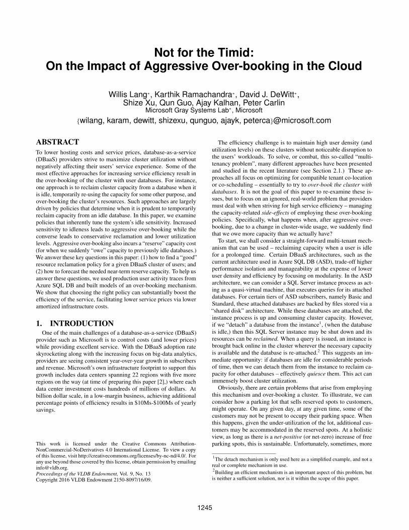
Figure 1: (a) Capacity (in core minutes) reclaimed and (b) re-served, along with (c) the observed DBs resumed per minutebased on different quiescence policy lengths over a three monthperiod from a production ASD cluster.

parking spots are being claimed than freed, a net-negative trend.As a result, the parking lot may need to dedicate some reservedcapacity to handle net-negative capacity changes. We address thisoft-ignored problem that arises in the context of DBaaS when weemploy quiescence techniques to over-book the cluster – a set re-serve capacity must be kept on hand for when quiesced DBs requireresources forcing them to be resumed.

In a cloud service like Azure SQL DB, there are generally periodsof ebb and flow in user activity (think weekends and holidays),where there are sustained periods of net-positive and net-negativequiescence. The problem that we (and the parking lots) have isthat we don’t know how long we should wait before we quiesce anidle DB and provide the capacity to some other DB. One straight-forward approach is to hypothesize that if the DB has been idle fora static amount of time, then it is likely to continue in this way andhence it is safe to quiesce. We can think of this duration of idle timeas being defined by the idleness based quiescence policy.

As the astute reader may already surmise, the quiescence pol-icy has a direct implication on the amount of reserve capacity thatmust be kept on hand, as well as the amount of capacity that wecan reclaim. Note however, that while the efficiency of the quiescemechanism may help mitigate this issue to some extent, the act ofover-booking itself creates the possibility of zero available capacitythat cannot be solved fully by any degree of mechanism improve-ment. Our first goal is therefore, given a production cluster (andusers), to find its “ideal” quiescence policy.

In Figure 1 we provide an example result from our analysis.These results are from a single cluster located in the US over a threemonth period ending 01/31/16 (results for additional clusters arepresented in Section 6). Here we used the production telemetry

data to determine user activity and idle periods as an input intoour quiescence model. For these results, we have employed eightdifferent quiescence policy lengths (the idle time required beforewe initiate the mechanism) from 1 hour to 7 days. The methodsby which we model the required reserve capacity are described inSections 4 and 5, but in essence, for each policy, we calculate theamount of net churn of DBs quiesced and resumed over the entirethree month period. As we model quiescence, we can determinehow much potential capacity we will reclaim with this mechanism.

Figures 1(a) and (b) contrast the potentially reclaimable capacity(in millions of CPU core minutes – a simplified metric for this paper),versus the reserve capacity required, respectively. As we shortenthe policy length from 7 days to 1 hour, we see in Figure 1(a) thatthe amount of capacity reclaimed increases – by almost 30% – fromabout 200 to 260 million CPU core minutes. Correspondingly, wealso see an increase in the required reserve capacity in Figure 1(b).Figure 1(c) shows the 99th percentile of all DBs resumed per minuteof the three month period given the real user activity. We see thatthe number of DBs resumed per minute climbs dramatically aswe shorten the policy length. This would increase the operationalcomplexity and may sometimes decrease user satisfaction.

To determine the “ideal” policy, we must normalize DBs re-sumed per minute so that we can come up with a single mea-sure per policy. We did this by conservatively assuming that, ifa DB is resumed more than five times in a month, (assuming a99.99% Azure SQL DB SLA [2],) then a capacity compensation (ofone month) will be provided. Consequently, we find the measure:net reclaim potential = (reclaim potential−reserve capacity−compensated capacity). In relation to Figure 1, we found thatfor this US cluster, the 1 day policy was the best out of these 8 op-tions and provided an 18% improvement over the worst performingpolicy, which was the 1 hour policy due to high compensation. Atscale, in the context of billions of dollars of global infrastructurecosts, choosing the right policy can swing service operating costsby tens or even hundreds of millions of dollars a year, and these aresavings which can be directly passed to customers.

As we will show, different clusters exhibit different activity pat-terns due in part to the population makeup. Therefore, none of thiswould do us any good if we aren’t able to continuously forecast,monitor, and adjust our reserve capacities in a production setting. Inthis paper, we will also discuss our second goal to develop a predic-tive model for the amount of reserve capacity and show the results ofevaluating our model. Our evaluations of historical production dataprovides penalty measures for various quiescence policies and fore-casting models which show us how well we would have done. Weemploy penalty measures such as a capacity outage when databasesare resumed but no reserve capacity is available (over-aggressiveforecasting) and unused reserve capacity (over-conservative fore-casting). Our three month evaluation can be found in Section 6.

To summarize, we make the following contributions in this paper.

• We introduce and formulate the oft-ignored problem due to over-booking DBaaS clusters: setting aside the right amount of reservecapacity and directly costing potential user impact.

• Using a quiescence mechanism, we define a tuning variable, apolicy analysis model, and various metrics that provide insightstowards answering the above problems.

• We present our analysis-backed solutions to two real-world prob-lems: how to find the ideal quiescence policy for our mechanismand how to periodically forecast the reserve capacity.

• We evaluate our solutions over extensive three month datasetsfrom two production clusters and present our results and findings.

1246

2. PRELIMINARIESTo begin, we discuss related work on the topic of database-as-a-

service followed by some background on the Azure SQL DB serviceas well as the telemetry data that we used.

2.1 Related WorkAlong with the sudden surge in adoption in data processing in the

cloud, we have also seen a swing in research towards the relevanttopics. The different approaches to cloud data processing can bebroadly divided by the different architectures [10]: shared hard-ware [4], shared table [1, 24], and finally the middle ground modelshared process [3, 22]. These different architectures trade isolationand manageability against properties such as density and efficiency.Azure SQL DB employs a different model – a process-centric modelthat focuses on performance and security isolation [3, 7, 21, 22].

On the topic of efficient multi-tenant scheduling and placement,there have been many methods and schemes discussed in the liter-ature [5, 6, 12, 13, 15, 16, 18, 20, 23]. While some of the placementschemes do not consider “over-booking” (as a consequence of aspecific cloud architecture), most of the tenant placement researchstrives to take advantage of underutilization or temporal contra-patterns, which inevitably leads to the problem that we have soldmore capacity than we actually have. Similarly, most of the schedul-ing research leans toward providing resources when they’re neededbut taking them away when they’re not. However, as we mentionedin Section 1, none of them consider the actual problem associatedwith over-booking, that is, what to do if we have used up all of ourcapacity and a user that was idle now demands resources?

The other aspect that has garnered significant attention is thatof efficient database migration mechanisms to allow placementreconfigurations and failovers [8, 11, 17]. Mechanisms such as theseare extremely important as to reduce latency of any capacity re-arragement. Ultimately effective full solutions must incorporatewell-designed mechanisms as well as the analysis framework thatwe focus on to determine the right policies to employ.

Other efforts more similar to ours deal with developing models onthe workloads to aid in the system’s decision-making. These includedeveloping machine learning models [9,25] or statistical models [19]to predict changes that the system must adapt to. However, none ofthese prior studies focus on our over-booked capacity problem, nordo they build and evaluate their models on the quality and quantityof production Azure SQL DB data that we have here.

2.2 Azure SQL DB ServiceWe now provide the basics of Microsoft’s Azure SQL DB service

necessary for this paper; additional information can be found at [2].Azure SQL DB operates on a process-oriented model where multiplecustomer databases may be co-located and served together via asingle (Azure) SQL Server process. Given that Azure SQL DB isrunning on SQL Server, many of the basic database managementconcepts of on-prem SQL Server remain available to the service.

Most notably, we could consider the SQL Server detach/attachmechanism (as an example mechanism for our purposes) that allowsa database to be “disconnected” from the SQL Server instanceprocess. After the database is detached, its physical files can bemoved or reattached by any other SQL Server instance and thedatabase will then consume resources provided by the new instance.

Note that this mechanism is not free. For example, detaching adatabase can take minutes or longer depending on the volume ofdirty memory pages in the buffer pool and I/O latency. Other factorscan influence the latency of a reattach as well and we account forthese (see Section 3.1.)

DB a unique identifier for the customer’s databaseslo the subscription t-shirt sizetimestamp the timespan from (timestamp − 15s) to timestampnode the node that the database resides onavg cpu the average cpu utilization (%)avg io the average I/O utilization (%)avg memory the average memory utilization (%)

Table 1: Telemetry Schema

Azure SQL Database currently offers a tiered subscription modelthat allows customers to choose from databases with different sub-scription levels, also known as ‘t-shirt’ sizes. T-shirt sizes corre-spond not only to various levels of performance, but also availability,and reliability objectives. Azure SQL Database’s current subscrip-tion model consists of three tiers: Basic, Standard, and Premium(Standard and Premium are further subdivided into four and threesub-level t-shirt sizes, respectively.)

The main difference that sets Premium databases apart is thefact that the physical data files are stored on the same node thathosts the SQL Server instance and not as files stored in AzureStorage volumes. This distinction provides immense benefits inperformance, but the Azure DB service must now manage physicaldata file replication on other Azure SQL DB nodes for availability.On the other hand, Basic and Standard tier databases are backed byphysical files stored on the Azure Storage layer, which performsreplication, thereby providing availability. For these two tiers, wecan attach and detach databases at will, changing the location of theSQL engine within the cluster. Databases subscribing to these twolower-cost tiers also make up the vast majority of all databases inthe service.

Finally, all of the t-shirt sizes come with performance SLOs thatessentially define the capacity requirements of a particular database.These are defined using a proprietary metric ‘database transactionunit’ (DTU), which is an internal transactional benchmark metric inthe spirit of TPC-C [2]. Internally, these DTUs map to traditionalCPU core, memory, and I/O bandwidth metrics. 3 In this paper, wewill frequently use CPU Cores as a normalizing capacity metric.

2.3 Telemetry DataIn this work, we relied upon the performance telemetry data to

tell us about an Azure SQL DB user’s activity. Instead of tellingus what queries were run, or how often they were issued, it tells usthe amount of CPU, memory, and I/O that was consumed by thisdatabase (in the process of executing queries.) The rough schema ofthe data is described by the column descriptions in Table 1.

This telemetry was collected from two Azure SQL DB clusters,one from the US and the other from Europe. The data is very similarto the telemetry described in [14], but it is of the current Azurearchitecture instead of the earlier version (v1) of Azure DB releasedin that paper. The main difference is that we now have data offiner granularity (records are emitted every 15 seconds instead ofevery 5 minutes) and generally, fewer anomalies are present. Ev-ery 15 seconds, every database could emit a row containing theresource utilization of that database during that timespan. Simi-lar to the prior data release, to reduce data volume, records arenot emitted if the database was completely idle (all three resourcemetrics were 0). This implies, for instance, that if we see tuple(db3, basic, 01/01/16 12:00:15, n38, 0.85, 0.20, 0.14) followed bytuple (db3, basic, 01/01/16 12:05:15, n38, 0.32, 0.19, 0.12), thendb3 was idle for five minutes.

3We will not disclose the exact mappings.

1247

2QUIESCESTATE

3QUIESCENT

STATE

1ACTIVESTATE

4RESUMESTATE

WhileQuiesce

WhileResuming

Ifpast_utilization(dbi,T)<>0

Ifnoresourcesrequested(e.g.,queries issued)

Ifpast_utilization(dbi,T)=0

Ifresourcesrequested(e.g.,data requested)

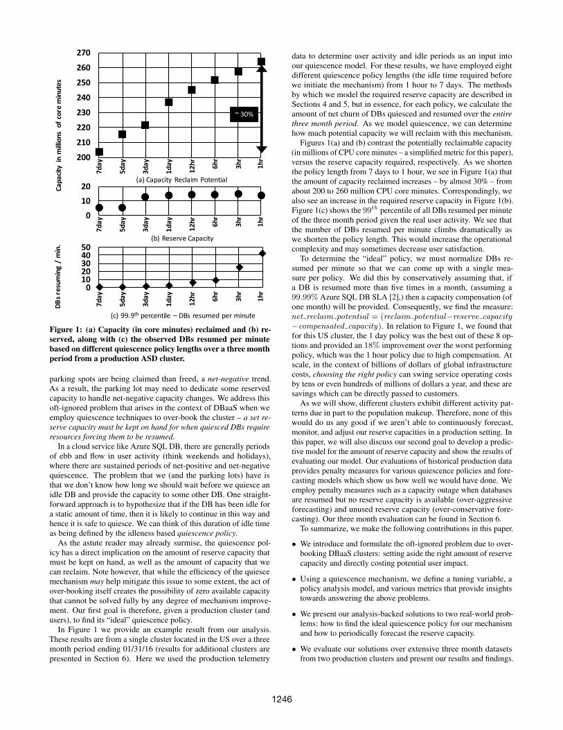
Figure 2: Quiescence State Diagram for some database dbi andpolicy length p. past utilization is a function that returns theutilization level of the dbi in the past T time.

3. PROBLEM FORMULATIONWe now formulate two capacity management problems involved

in the over-booking of database clusters. First, we will discuss amechanism that can be employed to over-book clusters, and then wewill describe the problems in the context of Azure SQL DB service.

3.1 Mechanism BackgroundThe quiesce mechanism that is relatively straight-forward to im-

plement (and think about) in SQL Server is the act of detaching adatabase.4 When the database is detached, it can no longer servicequeries as the database engine no longer has access to the data.When a database is detached, certain memory and log operationsmay need to be performed and/or completed. This includes memoryresident data checkpointing which can take a non-trivial amount oftime to complete (minutes or longer).

Conversely, if the user requests a data page from a quiescedDB, then it must be “resumed”, which would include invokingSQL Server’s database attach function. Similarly, this is not aninstantaneous action as the database’s physical files stored in the“shared disk” layer must be found, sufficient free capacity for theDB’s subscription tier must be found, and the attach itself performed.Therefore, both of the transitions – quiesce and resume – must beaccounted for.

Figure 2 illustrates the intuitive four-state state diagram for ourquiesce/resume workflow.

DEFINITION 3.1. A database can be modeled as being in one offour states: (1) Active; (2) Quiesce; (3) Quiescent; and (4) Resume.

In our model, databases remain in state 1 if there is any level ofutilization in the past T length timespan. If sufficient idleness isdetected, the db is transitioned to state 2 where it stays until thequiesce process is completed and it moves onto state 3. While thereare no requests of this database, it remains in the quiescent state.Once a database receives a request, it transitions to state 4 and staysthere until resume completes, at which point it returns to state 1.

4 Note that this detach/attach mechanism is only used here as a simplifiedexample, and is not a real or complete mechanism in use.

3.2 FormulationNow that we have described our mechanism, we can focus on the

problems associated with over-booking. Using the above mecha-nism, we may attempt to increase service efficiency by reclaimingcluster resources from databases that are idle (e.g., by detachingsuch databases), and using the reclaimed capacity to host moredatabases. A question that immediately arises here is: How do wedecide which databases should be detached? In other words, weneed a reasonable approach to identify the right quiesce candidates,hereafter referred to as the quiescence policy.

While there could be several quiescence policies possible, in thispaper we restrict ourselves to a set of policies based on the durationof idleness exhibited by databases. The idleness-based quiescencepolicy is defined as follows: A database is deemed to be a candidatefor quiesce if it exhibits continuous idleness for a specified durationT, which we call the quiescence policy length. The idleness-basedquiescence policy P is parameterized by the policy length T , andis based on the hypothesis that if a database has remained idle fortime T , it is likely to remain idle for a longer duration and hence, isa suitable quiesce candidate.

Enforcing a quiescence policy P (T ) involves quiescing the data-bases that are identified by the policy, thus freeing up the corre-sponding cluster resources. The amount of resources that wouldfree up as a result of applying policy P (T ) is referred to as thereclaim potential of P (T ). However, enforcing a quiescence policyalso implies that a fraction of the quiescent databases may have tobe resumed. There are continually databases being quiesced andresumed, so we care about the net churn in these databases. In thecase of negative net churn (where we are resuming more databasesthan we quiesce), we need to accommodate these resumed DBs byreserving certain cluster resources. The reserve capacity requiredin order to enforce a policy is essentially the capacity necessary forthe continuous swings in the net churn. The cost of maintaining thisreserve is the reserve capacity cost of P (T ).

Another important factor that needs to be considered is the re-sume cost. Resume incurs costs because they involve operationsthat include bringing back an instance online in the cluster whereverthe necessary capacity is available, and re-attaching the database toit. Too many DBs being resumed can increase operational complex-ity and may even lead to dissatisfied customers, and hence is notdesirable. Therefore, we account for the resume cost by taking avery conservative stance. We assume that if a database is resumedmore than 5 times in a month, (4.5min. with a simplified 1 minuteresume time,) it fails the 99.99% Azure SQL DB SLA [2], and hasto be compensated in capacity. The capacity compensation incurreddue to enforcing a policy is the resume cost of a policy P (T ).

Therefore, the total policy cost of a quiescence policy is the sumof its resume cost and the cost of the reserve capacity. Assumingthat this cost is fulfilled from the reclaim potential, we can arriveat the net reclaim potential of P (T ) by subtracting the total policycost from its reclaim potential.

net reclaim potential =reclaim potential

− reserve capacity cost

− resume cost

(1)

With the above notions, we are now ready to formulate the firstproblem we address in this paper.

PROBLEM 1. Determine the quiescence policy P (T ) that leadsto the maximum net reclaim potential.

Observe that there is a trade-off here, between the reclaim po-tential and the total policy cost. Analyzing and understanding the

1248

DBDROPDBCREATE

DBDROPDBCREATE

DBDROPDBCREATE

UTILIZA

TION

(e.g.,CPU)

TIME

TIME

TIME

ACTIVITY

IDLE

ACTIVE

QUIESCENTQUIESCE

RESUME

policyP(T) policyP(T)

RAW

TELEMETRY

BINA

RY

SIGN

ALSTAT

EMODE

L

Idleperiod1Idleperiod2

Idleperiod3

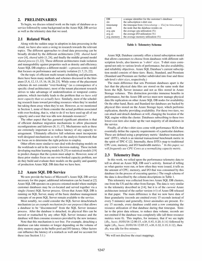
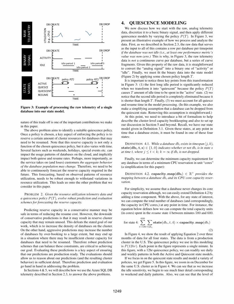
Figure 3: Example of processing the raw telemetry of a singledatabase into our state model.

nature of this trade off is one of the important contributions we makein this paper.

The above problem aims to identify a suitable quiescence policy.Once a policy is chosen, a key aspect of enforcing the policy is toreserve a certain amount of cluster resources for databases that mayneed to be resumed. Note that this reserve capacity is not only afunction of the chosen quiescence policy, but it also varies with time.Several factors such as weekends, holidays, special events etc. canimpact the usage patterns of databases on the cloud, and implicitlyimpact both quiese and resume rates. Perhaps, more importantly, asthe service takes on (and loses) customers the aggregate behaviorof the database population may change. Therefore, we need to beable to continuously forecast the reserve capacity required in thefuture. This forecasting, based on observed patterns of resourceutilization, needs to be robust enough to withstand variations inresource utilization. This leads us onto the other problem that weconsider in this paper.

PROBLEM 2. Given the resource utilization telemetry data anda quiescence policy P (T ), evolve robust prediction and evaluationschemes for forecasting the reserve capacity.

Predicting reserve capacity in a conservative manner may besafe in terms of reducing the resume cost. However, the downsideof conservative predictions is that it may result in reserve clustercapacity that may remain unused. This defeats the stated goal of ourwork, which is to increase the density of databases on the cluster.On the other hand, aggressive predictions may increase the numberof databases by over-booking to a large extent, but may end upin a situation where there may be insufficient cluster capacity fordatabases that need to be resumed. Therefore robust predictionschemes that can balance these constraints, are critical to achievingour goal. Evaluating these predictions is a key aspect of ensuringthat our predictions are production ready. The evaluations shouldallow us to reason about our predictions (and the resulting clusterbehavior) in sufficient detail. Therefore prediction and evaluationgo hand in hand in addressing the problem.

In Sections 4 & 5, we will describe how we use the Azure SQL DBtelemetry described in Section 2.3, to answer the above problems.

4. QUIESCENCE MODELINGWe now discuss how we start with the raw, analog telemetry

data, discretize it to a basic binary signal, and then apply differentquiescence models by varying the policy P (T ). In Figure 3, wepresent an illustrative example of how we process and analyze thedata. First, as we described in Section 2.3, the raw data that servesas the input to all of this contains a row per database per timepointif the database was not idle (i.e., at least one performance metric’svalue was non-zero.) This is why, in Figure 3, the raw telemetrydata is not a continuous curve per database, but a series of curvefragments. Given this property of the raw data, it is straightforwardto convert the “analog signal” into a binary one of “activity” or“idle”. Finally, we must fit the binary data into the state model(Figure 2) by applying some chosen policy length T .

It is important to notice three key points from this transformationin Figure 3: (1) the first long idle period is significantly reducedwhen we transform it into “quiescent” because the policy P (T )causes T amount of idle time to be spent in the ”active” state. (2) wenotice that the second idle period is completely eliminated because itis shorter than length T . Finally, (3) we must account for all quiesceand resume time in the model processing. (In this example, we alsomake a simplifying assumption that a database can be dropped fromthe quiescent state. Removing this assumption is straightforward.)

At this point, we need to introduce a bit of formalism to helpdescribe the cluster-level capacity bookkeeping and also to set upour discussion in Section 5 and beyond. Recall, we have our statemodel given in Definition 3.1. Given these states, at any point intime that a database exists, it must be found in one of these fourstates:

DEFINITION 4.1. While a database dbi exists in timespan [j, k),state(dbi, t, s) ∈ {1, 0} indicates whether or not dbi is in state sat time t, where j ≤ t < k; k =∞ if dbi is not dropped.

Finally, we can determine the minimum capacity requirement forany database in terms of a minimum CPU reservation in unit “cores”(a simplification for this paper):

DEFINITION 4.2. capacity map(dbi) ∈ R+ provides themapping between a database dbi and its CPU core capacity reser-vation.

For simplicity, we assume that a database never changes its corecapacity reservation although, we can easily extend Definition 4.2 byadding a time component. With the above, for any state of interest,we can compute the total number of databases (and correspondingly,the capacity in CPU cores,) at any point in time. For instance, theequation below defines how we can compute the total capacity units(in cores) spent in the resume state 4 between minutes 580 and 600.

for state 4:600∑

t=580

∑∀dbi

state(dbi, t, 4)× capacity map(dbi)

(2)In Figure 4, we show the result of applying Equation 2 over three

months of data for all four states. The data is from a productioncluster in the U.S. The quiescence policy we use in this modelingis P (12hr). Each point in the figure represents a single minute. Inthis figure, with a 12hr quiescence policy, we can readily see dailyand weekly patterns in both the Active and Quiescent state models.

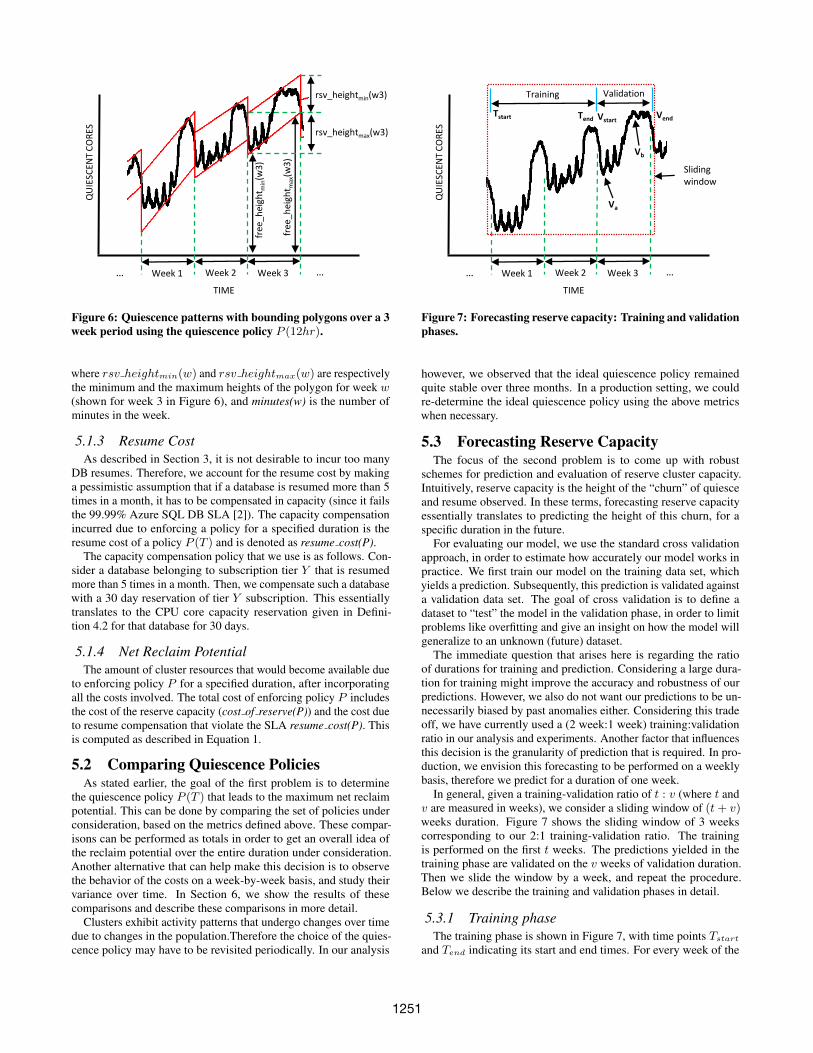
If we focus in on the quiescent state results and model a variety ofpolicies, we get Figure 5. In this figure, we zoom in on December forthe same U.S. cluster as in Figure 4. We can see that as we increasethe idle sensitivity, we begin to see much finer detail correspondingto weekend and daily patterns. Also, we can see that the level of

1249

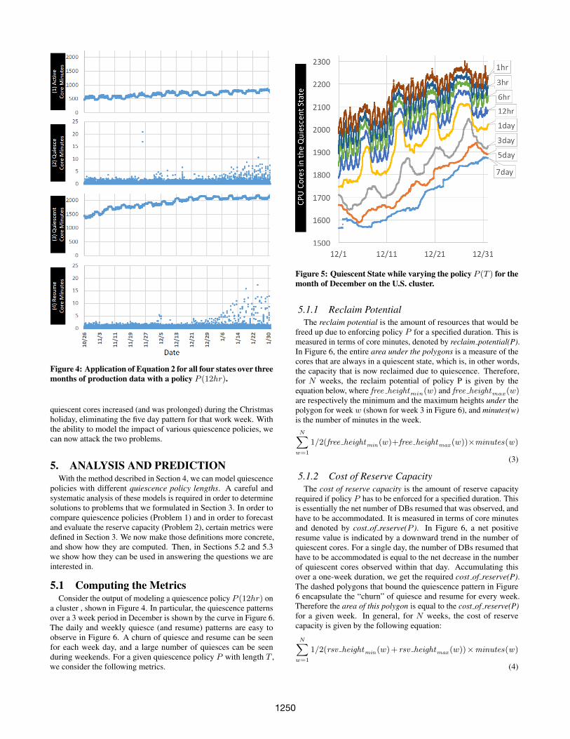
Figure 4: Application of Equation 2 for all four states over threemonths of production data with a policy P (12hr).

quiescent cores increased (and was prolonged) during the Christmasholiday, eliminating the five day pattern for that work week. Withthe ability to model the impact of various quiescence policies, wecan now attack the two problems.

5. ANALYSIS AND PREDICTIONWith the method described in Section 4, we can model quiescence

policies with different quiescence policy lengths. A careful andsystematic analysis of these models is required in order to determinesolutions to problems that we formulated in Section 3. In order tocompare quiescence policies (Problem 1) and in order to forecastand evaluate the reserve capacity (Problem 2), certain metrics weredefined in Section 3. We now make those definitions more concrete,and show how they are computed. Then, in Sections 5.2 and 5.3we show how they can be used in answering the questions we areinterested in.

5.1 Computing the MetricsConsider the output of modeling a quiescence policy P (12hr) on

a cluster , shown in Figure 4. In particular, the quiescence patternsover a 3 week period in December is shown by the curve in Figure 6.The daily and weekly quiesce (and resume) patterns are easy toobserve in Figure 6. A churn of quiesce and resume can be seenfor each week day, and a large number of quiesces can be seenduring weekends. For a given quiescence policy P with length T ,we consider the following metrics.

Figure 5: Quiescent State while varying the policy P (T ) for themonth of December on the U.S. cluster.

5.1.1 Reclaim PotentialThe reclaim potential is the amount of resources that would be

freed up due to enforcing policy P for a specified duration. This ismeasured in terms of core minutes, denoted by reclaim potential(P).In Figure 6, the entire area under the polygons is a measure of thecores that are always in a quiescent state, which is, in other words,the capacity that is now reclaimed due to quiescence. Therefore,for N weeks, the reclaim potential of policy P is given by theequation below, where free heightmin(w) and free heightmax(w)are respectively the minimum and the maximum heights under thepolygon for week w (shown for week 3 in Figure 6), and minutes(w)is the number of minutes in the week.N∑

w=1

1/2(free heightmin(w)+free heightmax (w))×minutes(w)

(3)

5.1.2 Cost of Reserve CapacityThe cost of reserve capacity is the amount of reserve capacity

required if policy P has to be enforced for a specified duration. Thisis essentially the net number of DBs resumed that was observed, andhave to be accommodated. It is measured in terms of core minutesand denoted by cost of reserve(P ). In Figure 6, a net positiveresume value is indicated by a downward trend in the number ofquiescent cores. For a single day, the number of DBs resumed thathave to be accommodated is equal to the net decrease in the numberof quiescent cores observed within that day. Accumulating thisover a one-week duration, we get the required cost of reserve(P).The dashed polygons that bound the quiescence pattern in Figure6 encapsulate the “churn” of quiesce and resume for every week.Therefore the area of this polygon is equal to the cost of reserve(P)for a given week. In general, for N weeks, the cost of reservecapacity is given by the following equation:

N∑w=1

1/2(rsv heightmin(w)+ rsv heightmax (w))×minutes(w)

(4)

1250

TIME

QU

IESC

ENT

CO

RES

Week 1 Week 2 Week 3… …fr

ee_h

eigh

t min

(w3

)

free

_hei

ght m

ax(w

3)

rsv_heightmin(w3)

rsv_heightmax(w3)

Figure 6: Quiescence patterns with bounding polygons over a 3week period using the quiescence policy P (12hr).

where rsv heightmin(w) and rsv heightmax(w) are respectivelythe minimum and the maximum heights of the polygon for week w(shown for week 3 in Figure 6), and minutes(w) is the number ofminutes in the week.

5.1.3 Resume CostAs described in Section 3, it is not desirable to incur too many

DB resumes. Therefore, we account for the resume cost by makinga pessimistic assumption that if a database is resumed more than 5times in a month, it has to be compensated in capacity (since it failsthe 99.99% Azure SQL DB SLA [2]). The capacity compensationincurred due to enforcing a policy for a specified duration is theresume cost of a policy P (T ) and is denoted as resume cost(P).

The capacity compensation policy that we use is as follows. Con-sider a database belonging to subscription tier Y that is resumedmore than 5 times in a month. Then, we compensate such a databasewith a 30 day reservation of tier Y subscription. This essentiallytranslates to the CPU core capacity reservation given in Defini-tion 4.2 for that database for 30 days.

5.1.4 Net Reclaim PotentialThe amount of cluster resources that would become available due

to enforcing policy P for a specified duration, after incorporatingall the costs involved. The total cost of enforcing policy P includesthe cost of the reserve capacity (cost of reserve(P)) and the cost dueto resume compensation that violate the SLA resume cost(P). Thisis computed as described in Equation 1.

5.2 Comparing Quiescence PoliciesAs stated earlier, the goal of the first problem is to determine

the quiescence policy P (T ) that leads to the maximum net reclaimpotential. This can be done by comparing the set of policies underconsideration, based on the metrics defined above. These compar-isons can be performed as totals in order to get an overall idea ofthe reclaim potential over the entire duration under consideration.Another alternative that can help make this decision is to observethe behavior of the costs on a week-by-week basis, and study theirvariance over time. In Section 6, we show the results of thesecomparisons and describe these comparisons in more detail.

Clusters exhibit activity patterns that undergo changes over timedue to changes in the population.Therefore the choice of the quies-cence policy may have to be revisited periodically. In our analysis

TIME

QU

IESC

ENT

CO

RES

Week 1 Week 2 Week 3… …

Training Validation

Va

Tstart

Sliding window

Vb

Tend VstartVend

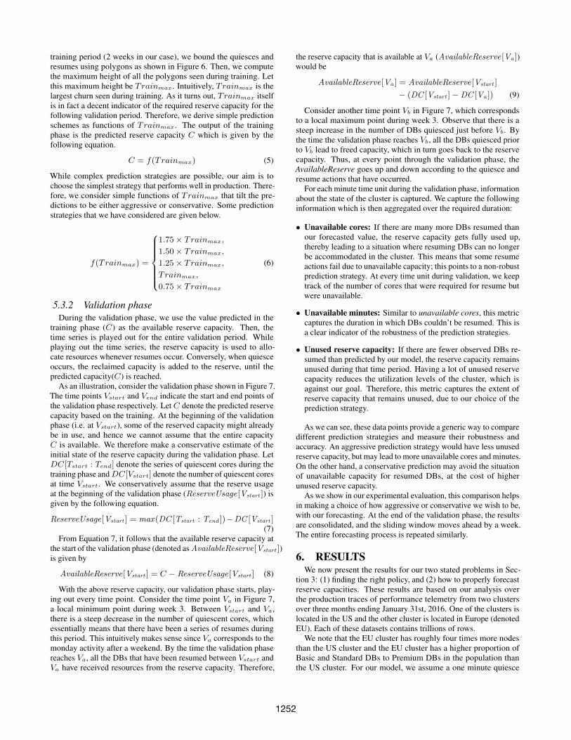
Figure 7: Forecasting reserve capacity: Training and validationphases.

however, we observed that the ideal quiescence policy remainedquite stable over three months. In a production setting, we couldre-determine the ideal quiescence policy using the above metricswhen necessary.

5.3 Forecasting Reserve CapacityThe focus of the second problem is to come up with robust

schemes for prediction and evaluation of reserve cluster capacity.Intuitively, reserve capacity is the height of the “churn” of quiesceand resume observed. In these terms, forecasting reserve capacityessentially translates to predicting the height of this churn, for aspecific duration in the future.

For evaluating our model, we use the standard cross validationapproach, in order to estimate how accurately our model works inpractice. We first train our model on the training data set, whichyields a prediction. Subsequently, this prediction is validated againsta validation data set. The goal of cross validation is to define adataset to “test” the model in the validation phase, in order to limitproblems like overfitting and give an insight on how the model willgeneralize to an unknown (future) dataset.

The immediate question that arises here is regarding the ratioof durations for training and prediction. Considering a large dura-tion for training might improve the accuracy and robustness of ourpredictions. However, we also do not want our predictions to be un-necessarily biased by past anomalies either. Considering this tradeoff, we have currently used a (2 week:1 week) training:validationratio in our analysis and experiments. Another factor that influencesthis decision is the granularity of prediction that is required. In pro-duction, we envision this forecasting to be performed on a weeklybasis, therefore we predict for a duration of one week.

In general, given a training-validation ratio of t : v (where t andv are measured in weeks), we consider a sliding window of (t+ v)weeks duration. Figure 7 shows the sliding window of 3 weekscorresponding to our 2:1 training-validation ratio. The trainingis performed on the first t weeks. The predictions yielded in thetraining phase are validated on the v weeks of validation duration.Then we slide the window by a week, and repeat the procedure.Below we describe the training and validation phases in detail.

5.3.1 Training phaseThe training phase is shown in Figure 7, with time points Tstart

and Tend indicating its start and end times. For every week of the

1251

training period (2 weeks in our case), we bound the quiesces andresumes using polygons as shown in Figure 6. Then, we computethe maximum height of all the polygons seen during training. Letthis maximum height be Trainmax. Intuitively, Trainmax is thelargest churn seen during training. As it turns out, Trainmax itselfis in fact a decent indicator of the required reserve capacity for thefollowing validation period. Therefore, we derive simple predictionschemes as functions of Trainmax. The output of the trainingphase is the predicted reserve capacity C which is given by thefollowing equation.

C = f(Trainmax) (5)

While complex prediction strategies are possible, our aim is tochoose the simplest strategy that performs well in production. There-fore, we consider simple functions of Trainmax that tilt the pre-dictions to be either aggressive or conservative. Some predictionstrategies that we have considered are given below.

f(Trainmax) =

1.75× Trainmax,

1.50× Trainmax,

1.25× Trainmax,

T rainmax,

0.75× Trainmax

(6)

5.3.2 Validation phaseDuring the validation phase, we use the value predicted in the

training phase (C) as the available reserve capacity. Then, thetime series is played out for the entire validation period. Whileplaying out the time series, the reserve capacity is used to allo-cate resources whenever resumes occur. Conversely, when quiesceoccurs, the reclaimed capacity is added to the reserve, until thepredicted capacity(C) is reached.

As an illustration, consider the validation phase shown in Figure 7.The time points Vstart and Vend indicate the start and end points ofthe validation phase respectively. Let C denote the predicted reservecapacity based on the training. At the beginning of the validationphase (i.e. at Vstart), some of the reserved capacity might alreadybe in use, and hence we cannot assume that the entire capacityC is available. We therefore make a conservative estimate of theinitial state of the reserve capacity during the validation phase. LetDC[Tstart : Tend] denote the series of quiescent cores during thetraining phase and DC[Vstart] denote the number of quiescent coresat time Vstart. We conservatively assume that the reserve usageat the beginning of the validation phase (ReserveUsage[Vstart ]) isgiven by the following equation.

ReserveUsage[Vstart ] = max (DC [Tstart : Tend ])−DC [Vstart ](7)

From Equation 7, it follows that the available reserve capacity atthe start of the validation phase (denoted as AvailableReserve[Vstart ])is given by

AvailableReserve[Vstart ] = C − ReserveUsage[Vstart ] (8)

With the above reserve capacity, our validation phase starts, play-ing out every time point. Consider the time point Va in Figure 7,a local minimum point during week 3. Between Vstart and Va,there is a steep decrease in the number of quiescent cores, whichessentially means that there have been a series of resumes duringthis period. This intuitively makes sense since Va corresponds to themonday activity after a weekend. By the time the validation phasereaches Va, all the DBs that have been resumed between Vstart andVa have received resources from the reserve capacity. Therefore,

the reserve capacity that is available at Va (AvailableReserve[Va ])would be

AvailableReserve[Va ] = AvailableReserve[Vstart ]

− (DC [Vstart ]−DC [Va ]) (9)

Consider another time point Vb in Figure 7, which correspondsto a local maximum point during week 3. Observe that there is asteep increase in the number of DBs quiesced just before Vb. Bythe time the validation phase reaches Vb, all the DBs quiesced priorto Vb lead to freed capacity, which in turn goes back to the reservecapacity. Thus, at every point through the validation phase, theAvailableReserve goes up and down according to the quiesce andresume actions that have occurred.

For each minute time unit during the validation phase, informationabout the state of the cluster is captured. We capture the followinginformation which is then aggregated over the required duration:

• Unavailable cores: If there are many more DBs resumed thanour forecasted value, the reserve capacity gets fully used up,thereby leading to a situation where resuming DBs can no longerbe accommodated in the cluster. This means that some resumeactions fail due to unavailable capacity; this points to a non-robustprediction strategy. At every time unit during validation, we keeptrack of the number of cores that were required for resume butwere unavailable.

• Unavailable minutes: Similar to unavailable cores, this metriccaptures the duration in which DBs couldn’t be resumed. This isa clear indicator of the robustness of the prediction strategies.

• Unused reserve capacity: If there are fewer observed DBs re-sumed than predicted by our model, the reserve capacity remainsunused during that time period. Having a lot of unused reservecapacity reduces the utilization levels of the cluster, which isagainst our goal. Therefore, this metric captures the extent ofreserve capacity that remains unused, due to our choice of theprediction strategy.

As we can see, these data points provide a generic way to comparedifferent prediction strategies and measure their robustness andaccuracy. An aggressive prediction strategy would have less unusedreserve capacity, but may lead to more unavailable cores and minutes.On the other hand, a conservative prediction may avoid the situationof unavailable capacity for resumed DBs, at the cost of higherunused reserve capacity.

As we show in our experimental evaluation, this comparison helpsin making a choice of how aggressive or conservative we wish to be,with our forecasting. At the end of the validation phase, the resultsare consolidated, and the sliding window moves ahead by a week.The entire forecasting process is repeated similarly.

6. RESULTSWe now present the results for our two stated problems in Sec-

tion 3: (1) finding the right policy, and (2) how to properly forecastreserve capacities. These results are based on our analysis overthe production traces of performance telemetry from two clustersover three months ending January 31st, 2016. One of the clusters islocated in the US and the other cluster is located in Europe (denotedEU). Each of these datasets contains trillions of rows.

We note that the EU cluster has roughly four times more nodesthan the US cluster and the EU cluster has a higher proportion ofBasic and Standard DBs to Premium DBs in the population thanthe US cluster. For our model, we assume a one minute quiesce

1252

(a) Reclaim Potential (US) (b) Cost of Reserve (US) (c) Resume Cost (US)

(d) Reclaim Potential (EU) (e) Cost of Reserve (EU) (f) Resume Cost (EU)

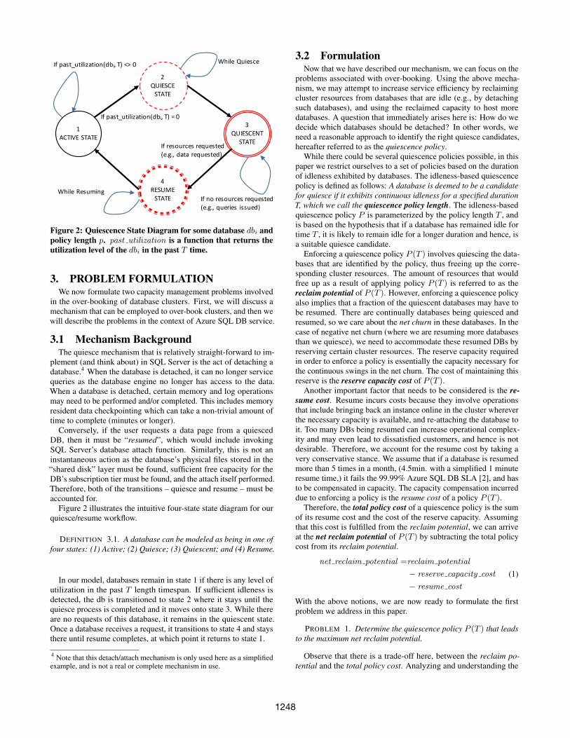
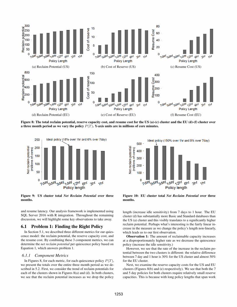
Figure 8: The total reclaim potential, reserve capacity cost, and resume cost for the US (a)-(c) cluster and the EU (d)-(f) cluster overa three month period as we vary the policy P (T ). Y-axis units are in millions of core minutes.

Figure 9: US cluster total Net Reclaim Potential over threemonths.

and resume latency. Our analysis framework is implemented usingSQL Server 2016 with R integration. Throughout the remainingdiscussion, we will highlight some key observations to take away.

6.1 Problem 1: Finding the Right PolicyIn Section 5.1, we described three different metrics for our quies-

cence model: the reclaim potential, the reserve capacity cost, andthe resume cost. By combining these 3 component metrics, we candetermine the net reclaim potential per quiescence policy based onEquation 1, which answers problem 1.

6.1.1 Component MetricsIn Figures 8, for each metric, for each quiescence policy P (T ),

we present the totals over the entire three month period as we de-scribed in 5.2. First, we consider the trend of reclaim potentials foreach of the clusters shown in Figures 8(a) and (d). In both clusters,we see that the reclaim potential increases as we drop the policy

Figure 10: EU cluster total Net Reclaim Potential over threemonths.

length (increase idle sensitivity) from 7 days to 1 hour. The EUcluster (d) has substantially more Basic and Standard databases thanthe US (a) cluster and this visibly translates to a significantly higherreclaim potential. Perhaps what’s interesting is the fairly linear in-crease in the measure as we change the policy’s length non-linearly,which leads us to our first observation.

Observation 1: The amount of reclaimable capacity increasesat a disproportionately higher rate as we decrease the quiescencepolicy (increase the idle sensitivity.)

However, we see that the rate of the increase in the reclaim po-tential between the two clusters is different: the relative differencebetween 7 day and 1 hour is 30% for the US cluster and almost 50%for the EU cluster.

Next, we examine the reserve capacity costs for the US and EUclusters (Figures 8(b) and (e) respectively). We see that both the 7and 5 day policies for both clusters require relatively small reservecapacities. This is because with long policy lengths that span work

1253

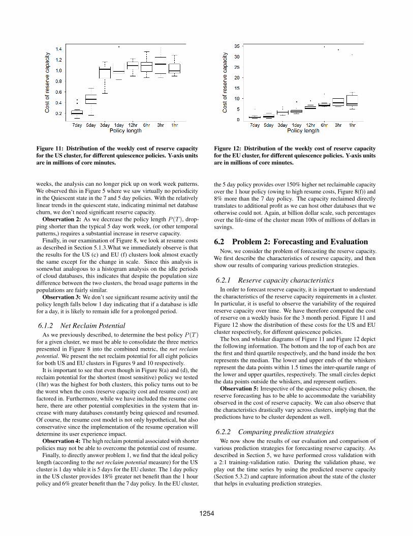
Figure 11: Distribution of the weekly cost of reserve capacityfor the US cluster, for different quiescence policies. Y-axis unitsare in millions of core minutes.

weeks, the analysis can no longer pick up on work week patterns.We observed this in Figure 5 where we saw virtually no periodicityin the Quiescent state in the 7 and 5 day policies. With the relativelylinear trends in the quiescent state, indicating minimal net databasechurn, we don’t need significant reserve capacity.

Observation 2: As we decrease the policy length P (T ), drop-ping shorter than the typical 5 day work week, (or other temporalpatterns,) requires a substantial increase in reserve capacity.

Finally, in our examination of Figure 8, we look at resume costsas described in Section 5.1.3.What we immediately observe is thatthe results for the US (c) and EU (f) clusters look almost exactlythe same except for the change in scale. Since this analysis issomewhat analogous to a histogram analysis on the idle periodsof cloud databases, this indicates that despite the population sizedifference between the two clusters, the broad usage patterns in thepopulations are fairly similar.

Observation 3: We don’t see significant resume activity until thepolicy length falls below 1 day indicating that if a database is idlefor a day, it is likely to remain idle for a prolonged period.

6.1.2 Net Reclaim PotentialAs we previously described, to determine the best policy P (T )

for a given cluster, we must be able to consolidate the three metricspresented in Figure 8 into the combined metric, the net reclaimpotential. We present the net reclaim potential for all eight policiesfor both US and EU clusters in Figures 9 and 10 respectively.

It is important to see that even though in Figure 8(a) and (d), thereclaim potential for the shortest (most sensitive) policy we tested(1hr) was the highest for both clusters, this policy turns out to bethe worst when the costs (reserve capacity cost and resume cost) arefactored in. Furthermore, while we have included the resume costhere, there are other potential complexities in the system that in-crease with many databases constantly being quiesced and resumed.Of course, the resume cost model is not only hypothetical, but alsoconservative since the implementation of the resume operation willdetermine its user experience impact.

Observation 4: The high reclaim potential associated with shorterpolicies may not be able to overcome the potential cost of resume.

Finally, to directly answer problem 1, we find that the ideal policylength (according to the net reclaim potential measure) for the UScluster is 1 day while it is 5 days for the EU cluster. The 1 day policyin the US cluster provides 18% greater net benefit than the 1 hourpolicy and 6% greater benefit than the 7 day policy. In the EU cluster,

Figure 12: Distribution of the weekly cost of reserve capacityfor the EU cluster, for different quiescence policies. Y-axis unitsare in millions of core minutes.

the 5 day policy provides over 150% higher net reclaimable capacityover the 1 hour policy (owing to high resume costs, Figure 8(f)) and8% more than the 7 day policy. The capacity reclaimed directlytranslates to additional profit as we can host other databases that weotherwise could not. Again, at billion dollar scale, such percentagesover the life-time of the cluster mean 100s of millions of dollars insavings.

6.2 Problem 2: Forecasting and EvaluationNow, we consider the problem of forecasting the reserve capacity.

We first describe the characteristics of reserve capacity, and thenshow our results of comparing various prediction strategies.

6.2.1 Reserve capacity characteristicsIn order to forecast reserve capacity, it is important to understand

the characteristics of the reserve capacity requirements in a cluster.In particular, it is useful to observe the variability of the requiredreserve capacity over time. We have therefore computed the costof reserve on a weekly basis for the 3 month period. Figure 11 andFigure 12 show the distribution of these costs for the US and EUcluster respectively, for different quiescence policies.

The box and whisker diagrams of Figure 11 and Figure 12 depictthe following information. The bottom and the top of each box arethe first and third quartile respectively, and the band inside the boxrepresents the median. The lower and upper ends of the whiskersrepresent the data points within 1.5 times the inter-quartile range ofthe lower and upper quartiles, respectively. The small circles depictthe data points outside the whiskers, and represent outliers.

Observation 5: Irrespective of the quiescence policy chosen, thereserve forecasting has to be able to accommodate the variabilityobserved in the cost of reserve capacity. We can also observe thatthe characteristics drastically vary across clusters, implying that thepredictions have to be cluster dependent as well.

6.2.2 Comparing prediction strategiesWe now show the results of our evaluation and comparison of

various prediction strategies for forecasting reserve capacity. Asdescribed in Section 5, we have performed cross validation witha 2:1 training-validation ratio. During the validation phase, weplay out the time series by using the predicted reserve capacity(Section 5.3.2) and capture information about the state of the clusterthat helps in evaluating prediction strategies.

1254

(a) Unavailable Cores (US) (b) Unavailable Minutes (US) (c) Unused Reserve (US)

(d) Unavailable Cores (EU) (e) Unavailable Minutes (EU) (f) Unused Reserve (EU)

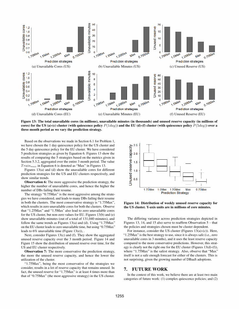
Figure 13: The total unavailable cores (in millions), unavailable minutes (in thousands) and unused reserve capacity (in millions ofcores) for the US (a)-(c) cluster (with quiescence policy P (1day)) and the EU (d)-(f) cluster (with quiescence policy P (5day)) over athree month period as we vary the prediction strategy.

Based on the observations we made in Section 6.1 for Problem 1,we have chosen the 1 day quiescence policy for the US cluster andthe 5 day quiescence policy for the EU cluster. We have considered5 prediction strategies as given by Equation 6. Figures 13 show theresults of comparing the 5 strategies based on the metrics given inSection 5.3.2, aggregated over the entire 3 month period. The valueTrainmax in Equation 6 is denoted as “Max” in Figures 13.

Figures 13(a) and (d) show the unavailable cores for differentprediction strategies for the US and EU clusters respectively, andshow similar trends.

Observation 6: The more aggressive the prediction strategy, thehigher the number of unavailable cores, and hence the higher thenumber of DBs failing their resume.

The strategy “0.75Max” is the most aggressive among the strate-gies we have considered, and leads to many DBs failing their resumein both the clusters. The most conservative strategy is “1.75Max”,which results in zero unavailable cores for both the clusters. Observethat “1.25Max” and “1.5Max’ also lead to zero unavailable coresfor the US cluster, but non-zero values for EU. Figures 13(b) and (e)show unavailable minutes (out of a total of 131,040 minutes), andfollow the same trends as Figures 13(a) and (d). Using “1.75Max”on the EU cluster leads to zero unavailable time, but using “0.75Max”leads to 6% unavailable time (Figure 13(e)), .

Next, consider Figures 13(c) and (f). They show the aggregatedunused reserve capacity over the 3 month period. Figure 14 andFigure 15 show the distribution of unused reserve over time, for theUS and EU cluster respectively.

Observation 7: The more conservative the prediction strategy,the more the unused reserve capacity, and hence the lower theutilization of the cluster.

“1.75Max”, being the most conservative of the strategies weconsider, results in a lot of reserve capacity that remains unused. Infact, the unused reserve for “1.75Max” is at least 4 times more thanthat of “0.75Max” (the most aggressive strategy) in the US cluster.

Figure 14: Distribution of weekly unused reserve capacity forthe US cluster. Y-axis units are in millions of core minutes.

The differing variance across prediction strategies depicted inFigures 13, 14, and 15 also serve to reaffirm Observation 5 – thatthe policies and strategies chosen must be cluster dependent.

For instance, consider the US cluster (Figures 13(a)-(c)). Here,“1.25Max” is the best strategy to use, since it is always safe (i.e., zerounavailable cores in 3 months), and it uses the least reserve capacitycompared to the more conservative predictions. However, this strat-egy is clearly not the right one for the EU cluster (Figures 13(d)-(f)),where “1.75Max” is the safest strategy. Also, observe that “Max”itself is not a safe enough forecast for either of the clusters. This isnot surprising, given the growing number of DBaaS adoptions.

7. FUTURE WORKIn the context of this work, we believe there are at least two main

categories of future work: (1) complex quiescence policies; and (2)

1255

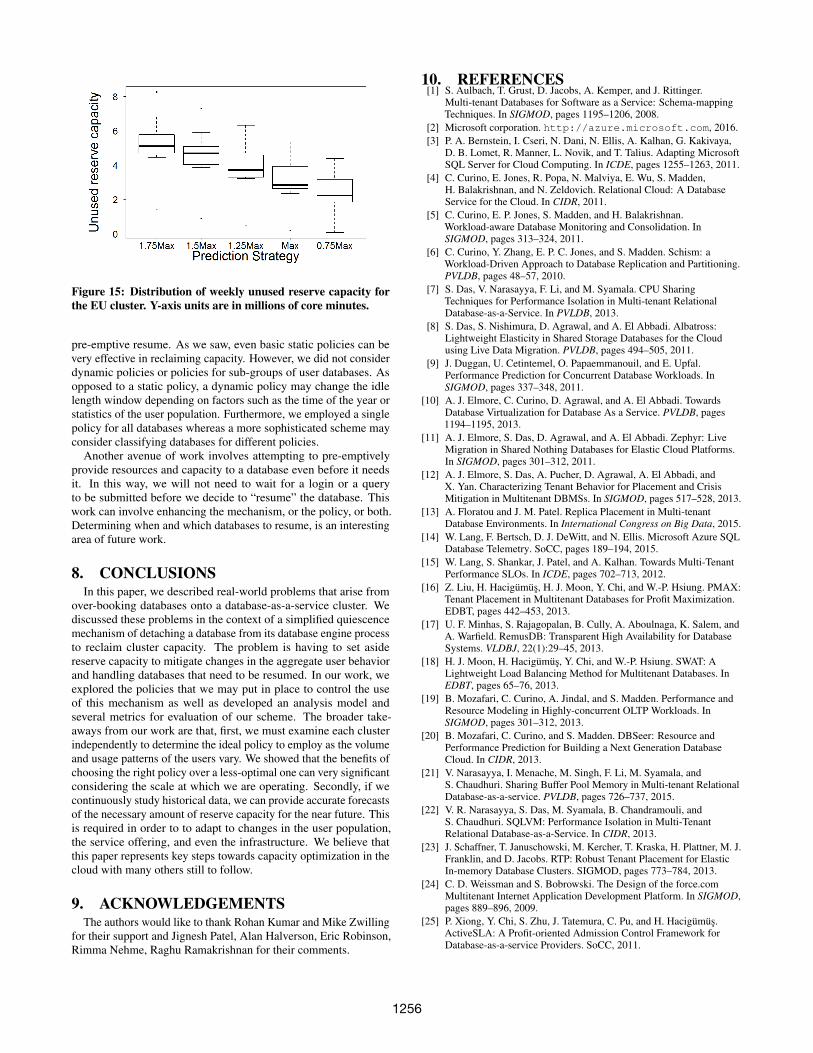
Figure 15: Distribution of weekly unused reserve capacity forthe EU cluster. Y-axis units are in millions of core minutes.

pre-emptive resume. As we saw, even basic static policies can bevery effective in reclaiming capacity. However, we did not considerdynamic policies or policies for sub-groups of user databases. Asopposed to a static policy, a dynamic policy may change the idlelength window depending on factors such as the time of the year orstatistics of the user population. Furthermore, we employed a singlepolicy for all databases whereas a more sophisticated scheme mayconsider classifying databases for different policies.

Another avenue of work involves attempting to pre-emptivelyprovide resources and capacity to a database even before it needsit. In this way, we will not need to wait for a login or a queryto be submitted before we decide to “resume” the database. Thiswork can involve enhancing the mechanism, or the policy, or both.Determining when and which databases to resume, is an interestingarea of future work.

8. CONCLUSIONSIn this paper, we described real-world problems that arise from

over-booking databases onto a database-as-a-service cluster. Wediscussed these problems in the context of a simplified quiescencemechanism of detaching a database from its database engine processto reclaim cluster capacity. The problem is having to set asidereserve capacity to mitigate changes in the aggregate user behaviorand handling databases that need to be resumed. In our work, weexplored the policies that we may put in place to control the useof this mechanism as well as developed an analysis model andseveral metrics for evaluation of our scheme. The broader take-aways from our work are that, first, we must examine each clusterindependently to determine the ideal policy to employ as the volumeand usage patterns of the users vary. We showed that the benefits ofchoosing the right policy over a less-optimal one can very significantconsidering the scale at which we are operating. Secondly, if wecontinuously study historical data, we can provide accurate forecastsof the necessary amount of reserve capacity for the near future. Thisis required in order to to adapt to changes in the user population,the service offering, and even the infrastructure. We believe thatthis paper represents key steps towards capacity optimization in thecloud with many others still to follow.

9. ACKNOWLEDGEMENTSThe authors would like to thank Rohan Kumar and Mike Zwilling

for their support and Jignesh Patel, Alan Halverson, Eric Robinson,Rimma Nehme, Raghu Ramakrishnan for their comments.

10. REFERENCES[1] S. Aulbach, T. Grust, D. Jacobs, A. Kemper, and J. Rittinger.

Multi-tenant Databases for Software as a Service: Schema-mappingTechniques. In SIGMOD, pages 1195–1206, 2008.

[2] Microsoft corporation. http://azure.microsoft.com, 2016.[3] P. A. Bernstein, I. Cseri, N. Dani, N. Ellis, A. Kalhan, G. Kakivaya,

D. B. Lomet, R. Manner, L. Novik, and T. Talius. Adapting MicrosoftSQL Server for Cloud Computing. In ICDE, pages 1255–1263, 2011.

[4] C. Curino, E. Jones, R. Popa, N. Malviya, E. Wu, S. Madden,H. Balakrishnan, and N. Zeldovich. Relational Cloud: A DatabaseService for the Cloud. In CIDR, 2011.

[5] C. Curino, E. P. Jones, S. Madden, and H. Balakrishnan.Workload-aware Database Monitoring and Consolidation. InSIGMOD, pages 313–324, 2011.

[6] C. Curino, Y. Zhang, E. P. C. Jones, and S. Madden. Schism: aWorkload-Driven Approach to Database Replication and Partitioning.PVLDB, pages 48–57, 2010.

[7] S. Das, V. Narasayya, F. Li, and M. Syamala. CPU SharingTechniques for Performance Isolation in Multi-tenant RelationalDatabase-as-a-Service. In PVLDB, 2013.

[8] S. Das, S. Nishimura, D. Agrawal, and A. El Abbadi. Albatross:Lightweight Elasticity in Shared Storage Databases for the Cloudusing Live Data Migration. PVLDB, pages 494–505, 2011.

[9] J. Duggan, U. Cetintemel, O. Papaemmanouil, and E. Upfal.Performance Prediction for Concurrent Database Workloads. InSIGMOD, pages 337–348, 2011.

[10] A. J. Elmore, C. Curino, D. Agrawal, and A. El Abbadi. TowardsDatabase Virtualization for Database As a Service. PVLDB, pages1194–1195, 2013.

[11] A. J. Elmore, S. Das, D. Agrawal, and A. El Abbadi. Zephyr: LiveMigration in Shared Nothing Databases for Elastic Cloud Platforms.In SIGMOD, pages 301–312, 2011.

[12] A. J. Elmore, S. Das, A. Pucher, D. Agrawal, A. El Abbadi, andX. Yan. Characterizing Tenant Behavior for Placement and CrisisMitigation in Multitenant DBMSs. In SIGMOD, pages 517–528, 2013.

[13] A. Floratou and J. M. Patel. Replica Placement in Multi-tenantDatabase Environments. In International Congress on Big Data, 2015.

[14] W. Lang, F. Bertsch, D. J. DeWitt, and N. Ellis. Microsoft Azure SQLDatabase Telemetry. SoCC, pages 189–194, 2015.

[15] W. Lang, S. Shankar, J. Patel, and A. Kalhan. Towards Multi-TenantPerformance SLOs. In ICDE, pages 702–713, 2012.

[16] Z. Liu, H. Hacigumus, H. J. Moon, Y. Chi, and W.-P. Hsiung. PMAX:Tenant Placement in Multitenant Databases for Profit Maximization.EDBT, pages 442–453, 2013.

[17] U. F. Minhas, S. Rajagopalan, B. Cully, A. Aboulnaga, K. Salem, andA. Warfield. RemusDB: Transparent High Availability for DatabaseSystems. VLDBJ, 22(1):29–45, 2013.

[18] H. J. Moon, H. Hacigumus, Y. Chi, and W.-P. Hsiung. SWAT: ALightweight Load Balancing Method for Multitenant Databases. InEDBT, pages 65–76, 2013.

[19] B. Mozafari, C. Curino, A. Jindal, and S. Madden. Performance andResource Modeling in Highly-concurrent OLTP Workloads. InSIGMOD, pages 301–312, 2013.

[20] B. Mozafari, C. Curino, and S. Madden. DBSeer: Resource andPerformance Prediction for Building a Next Generation DatabaseCloud. In CIDR, 2013.

[21] V. Narasayya, I. Menache, M. Singh, F. Li, M. Syamala, andS. Chaudhuri. Sharing Buffer Pool Memory in Multi-tenant RelationalDatabase-as-a-service. PVLDB, pages 726–737, 2015.

[22] V. R. Narasayya, S. Das, M. Syamala, B. Chandramouli, andS. Chaudhuri. SQLVM: Performance Isolation in Multi-TenantRelational Database-as-a-Service. In CIDR, 2013.

[23] J. Schaffner, T. Januschowski, M. Kercher, T. Kraska, H. Plattner, M. J.Franklin, and D. Jacobs. RTP: Robust Tenant Placement for ElasticIn-memory Database Clusters. SIGMOD, pages 773–784, 2013.

[24] C. D. Weissman and S. Bobrowski. The Design of the force.comMultitenant Internet Application Development Platform. In SIGMOD,pages 889–896, 2009.

[25] P. Xiong, Y. Chi, S. Zhu, J. Tatemura, C. Pu, and H. Hacigumus.ActiveSLA: A Profit-oriented Admission Control Framework forDatabase-as-a-service Providers. SoCC, 2011.

1256