Nonlinear, Transient Conduction Heat Transfer UsingA Discontinuous Galerkin Hierarchical Finite Element

Method

byJerome Charles Sanders

B.S. in Physics, May 2002The College of New Jersey

A Thesis submitted toThe faculty of

The School of Engineering and Applied Science ofThe George Washington University

in partial satisfaction of the requirements for the degree ofMaster of Science

August 31, 2004

This research was conducted at NASA’s Langley Research Center

Abstract

Hypersonic and reentry vehicles are exposed to high temperatures and large tempera-

ture gradients as they travel through the atmosphere. Previous launch vehicles relied on

thermal protection systems (TPS) to handle thermal loads while the structure supported

aerodynamic loads. Future launch vehicle designs will likely use non-insulated hot struc-

tures and multifunctional structures that sustain both thermal and aerodynamic loads

simultaneously. Finite element methods are needed to predict accurately the thermal

and structural response of these types of structures.

Due to the large temperature ranges encountered by hypersonic and reentry vehicles,

the thermal conductivity of the material must be considered temperature-dependent.

Current methods used to account for this temperature-dependence assume thermal con-

ductivity is constant over each element or alternatively, the finite element integrals con-

taining the thermal conductivity are integrated using Gaussian quadrature. These meth-

ods require a large number of elements or an excessive number of integration points,

respectively, to achieve satisfactory accuracy.

A hierarchical p-version space-time finite element method with a structurally compat-

ible mesh for nonlinear, transient problems is presented in this research. A hierarchical

finite element scheme with structurally compatible elements is used in space. A discon-

tinuous Galerkin time stepping scheme is used as the finite element method in time. An

optimized interpolation of the temperature-dependent thermal conductivity eliminates

the need for a large number of elements or an excessive number of integration points

and provides increased computational efficiency by utilizing master matrices. The finite

element formulation is tested and validated using sample problems. This finite element

formulation is shown to have the same theoretical convergence rates as those expected

for linear problems when a single source of error in the approximation can be isolated.

i

Acknowledgements

I would like to thank Dr. Kim Bey of the Metals and Thermal Structures Branch at

NASA’s Langley Research Center. Her patience, knowledge, and guidance were invalu-

able to my research. I would also like to thank Dr. Paul Cooper from the George

Washington University for his unique perspective and for his helpful insights into my

work. My thanks also go to Dr. Stephen Scotti for allowing me the opportunity to work

in the Metals and Thermal Structures Branch. Finally, I would like to thank my family

for their encouragement and support.

ii

Contents

Abstract . . . . . . . . . . . . . . . . . . . . . . . . . . . . . . . . . . . . . . . i

Acknowledgements . . . . . . . . . . . . . . . . . . . . . . . . . . . . . . . . . ii

Nomenclature . . . . . . . . . . . . . . . . . . . . . . . . . . . . . . . . . . . . xi

1 Introduction 1

1.1 Review of Previous Work . . . . . . . . . . . . . . . . . . . . . . . . . . . 4

1.2 Purpose . . . . . . . . . . . . . . . . . . . . . . . . . . . . . . . . . . . . 5

1.3 Scope . . . . . . . . . . . . . . . . . . . . . . . . . . . . . . . . . . . . . 6

2 Finite Element Method 7

2.1 Initial Boundary Value Problem . . . . . . . . . . . . . . . . . . . . . . . 7

2.2 Weak Formulation . . . . . . . . . . . . . . . . . . . . . . . . . . . . . . 9

2.3 Finite Element Formulation . . . . . . . . . . . . . . . . . . . . . . . . . 11

2.3.1 Discontinuous Galerkin Method in Time . . . . . . . . . . . . . . 14

2.3.2 Approximation of Solution . . . . . . . . . . . . . . . . . . . . . . 15

2.3.3 Temperature Approximation . . . . . . . . . . . . . . . . . . . . . 17

2.3.4 Temperature-Dependent Thermal Conductivity . . . . . . . . . . 20

2.4 Element Matrices . . . . . . . . . . . . . . . . . . . . . . . . . . . . . . . 21

2.5 Time-Stepping Solution Method . . . . . . . . . . . . . . . . . . . . . . . 24

2.6 Applying Initial and Boundary Conditions . . . . . . . . . . . . . . . . . 26

iii

3 Basis Functions 29

3.1 Time Basis Functions . . . . . . . . . . . . . . . . . . . . . . . . . . . . . 29

3.2 Through-Thickness Basis Functions . . . . . . . . . . . . . . . . . . . . . 31

3.3 Hierarchical In-Plane Basis Functions . . . . . . . . . . . . . . . . . . . . 35

4 Interpolation of Thermal Conductivity 47

4.1 Lagrange Interpolation Functions . . . . . . . . . . . . . . . . . . . . . . 48

4.1.1 Time Interpolation Functions . . . . . . . . . . . . . . . . . . . . 48

4.1.2 Through-Thickness Interpolation Functions . . . . . . . . . . . . . 50

4.1.3 In-Plane Interpolation Functions . . . . . . . . . . . . . . . . . . 50

4.2 Optimization of Sampling Points . . . . . . . . . . . . . . . . . . . . . . 54

4.3 Determination of Interpolation Coefficients . . . . . . . . . . . . . . . . . 55

4.4 Convergence Criteria for Iteration . . . . . . . . . . . . . . . . . . . . . . 58

5 Computer Implementation 60

5.1 Integration . . . . . . . . . . . . . . . . . . . . . . . . . . . . . . . . . . . 62

5.2 Master Element Matrices . . . . . . . . . . . . . . . . . . . . . . . . . . . 63

5.3 Enforcing Essential Boundary Conditions . . . . . . . . . . . . . . . . . . 69

6 Numerical Results 72

6.1 Error Convergence Estimates . . . . . . . . . . . . . . . . . . . . . . . . 72

6.2 Error Due to Fixed-Point Iteration . . . . . . . . . . . . . . . . . . . . . 76

6.3 Sample Problems . . . . . . . . . . . . . . . . . . . . . . . . . . . . . . . 77

6.3.1 Example 1 . . . . . . . . . . . . . . . . . . . . . . . . . . . . . . . 79

6.3.2 Example 2 . . . . . . . . . . . . . . . . . . . . . . . . . . . . . . . 83

6.3.3 Example 3 . . . . . . . . . . . . . . . . . . . . . . . . . . . . . . . 87

6.3.4 Example 4 . . . . . . . . . . . . . . . . . . . . . . . . . . . . . . . 92

iv

6.3.5 Example 5 . . . . . . . . . . . . . . . . . . . . . . . . . . . . . . . 97

6.3.6 Example 6 . . . . . . . . . . . . . . . . . . . . . . . . . . . . . . . 100

7 Concluding Remarks 105

References 108

v

List of Figures

2.1 Three-dimensional spatial domain, Ω, with Dirichlet and Neumann bound-

ary conditions . . . . . . . . . . . . . . . . . . . . . . . . . . . . . . . . . 8

2.2 Space-time mesh . . . . . . . . . . . . . . . . . . . . . . . . . . . . . . . 12

2.3 Discontinuous Solution in Time . . . . . . . . . . . . . . . . . . . . . . . 15

2.4 Arbitrary Two-Dimensional Spatial Domain with a Uniform Thickness . 17

2.5 Time-Stepping Solution Flowchart . . . . . . . . . . . . . . . . . . . . . . 25

3.1 Three-Dimensional Domain Collapsed onto a Two-Dimensional Mesh . . 32

3.2 One-dimensional hierarchical element . . . . . . . . . . . . . . . . . . . . 32

3.3 Local Basis Functions for ptk = 5 . . . . . . . . . . . . . . . . . . . . . . 33

3.4 Triangular Hierarchical Element Node Numbering Convention . . . . . . 35

3.5 Global Coordinates and Areas for a Triangle . . . . . . . . . . . . . . . . 36

3.6 Triangular Elements Sharing a Side . . . . . . . . . . . . . . . . . . . . . 40

4.1 Sample Time Lagrange Element . . . . . . . . . . . . . . . . . . . . . . . 49

4.2 In-Plane Lagrange Nodal Positions for rip = 3 (left) and rip = 5 (right) . 52

4.3 Fekete Points for In-Plane Degrees of Interpolation rip = 3, 6, 9 . . . . . . 55

5.1 Operational Order of ndgSCHTp . . . . . . . . . . . . . . . . . . . . . . 61

5.2 Extraction of Sub-Matrix from Master Time Mass Matrix . . . . . . . . . 65

5.3 Extraction of Element Basis Functions from Master In-Plane Basis . . . . 66

vi

5.4 Extraction of Sub-Matrix from Master In-Plane Matrix . . . . . . . . . . 67

5.5 Sample Element with Varying Degrees of Through-Thickness Approximation 68

5.6 Three-Dimensional Domain with Surface and Edge Boundary Conditions 69

6.1 Error Convergence Estimates on a Log-Log Scale

(a) H1 Error vs. Element Size

(b) L2 Error vs. Number of Time Steps . . . . . . . . . . . . . . . . . . . 76

6.2 2, 8, 16, and 32 Element In-plane Meshes . . . . . . . . . . . . . . . . . . 78

6.3 Exact Solution and Finite Element Error for Example 1 at t = 1s

(a) Exact solution

(b) Point-wise error with pip = rip = 5 and pt = rt = 1 . . . . . . . . . . . 80

6.4 Convergence of the Error for Example 1

(a) H1 Error for Different Values of pip

(b) L2 Error for Different Values of pip

(c) H1 Error for Different Values of rip

(d) L2 Error for Different Values of rip . . . . . . . . . . . . . . . . . . . 81

6.5 Exact Solution and Finite Element Error for Example 2 at t = 2s

(a) Exact solution

(b) Point-wise error with pip = rip = 4 and pt = rt = 6 using one time step 84

6.6 Example 2: H1 Error as a Function of Time for pt = 1 and pt = 4 . . . . 85

6.7 Convergence of the L2 Error for Example 2

(a) The Effect of Different Values of pt

(b) The Effect of Different Values of rt . . . . . . . . . . . . . . . . . . . 86

6.8 Exact Solution and Finite Element Error for Example 3 at t = 10s

(a) Exact solution

(b) Point-wise error with pip = rip = 4, pt = rt = 1, and ptk = rtk = 6 . . 89

vii

6.9 Convergence of the Error for Example 3

(a) H1 Error for Different Values of pip

(b) L2 Error for Different Values of pip

(c) H1 Error for Different Values of ptk

(d) L2 Error for Different Values of ptk . . . . . . . . . . . . . . . . . . . 91

6.10 Exact Solution and Finite Element Error for Example 4 at t = 1s

(a) Exact solution

(b) Point-wise error with pip = 3, rip = 6, pt = 2 and rt = 4 . . . . . . . . 93

6.11 Convergence of the Error for Example 4

(a) H1 Error for Different Values of pip

(b) L2 Error for Different Values of pip

(c) H1 Error for Different Values of rip

(d) L2 Error for Different Values of rip

(e) H1 Error for the Tabulation of Thermal Conductivity

(f) L2 Error for the Tabulation of Thermal Conductivity . . . . . . . . . 95

6.12 Exact Solution and Finite Element Error for Example 5 at t = 1s

(a) Exact solution

(b) Point-wise error with pip = rip = 5 and pt = rt = 6 using five time steps 98

6.13 Convergence of the L2 Error for Example 5

(a) The Effect of Different Values of pt

(b) The Effect of Different Values of rt . . . . . . . . . . . . . . . . . . . 99

6.14 Exact Solution and Finite Element Error for Example 6 at t = 1s

(a) Exact solution

(b) Point-wise error using a 16 element mesh and 5 time steps with pip =

rip = 6 and pt = rt = 4 . . . . . . . . . . . . . . . . . . . . . . . . . . . . 101

viii

6.15 Convergence of the Error for Example 6

(a) H1 Error as a Function of Time

(b) L2 Error for Different Values of pt

(c) H1 Error for Different Values of pip

(d) L2 Error for Different Values of pip . . . . . . . . . . . . . . . . . . . 102

ix

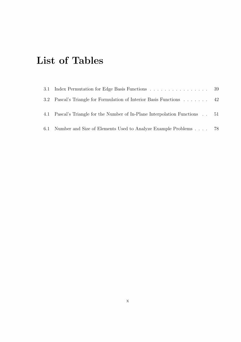
List of Tables

3.1 Index Permutation for Edge Basis Functions . . . . . . . . . . . . . . . . 39

3.2 Pascal’s Triangle for Formulation of Interior Basis Functions . . . . . . . 42

4.1 Pascal’s Triangle for the Number of In-Plane Interpolation Functions . . 51

6.1 Number and Size of Elements Used to Analyze Example Problems . . . . 78

x

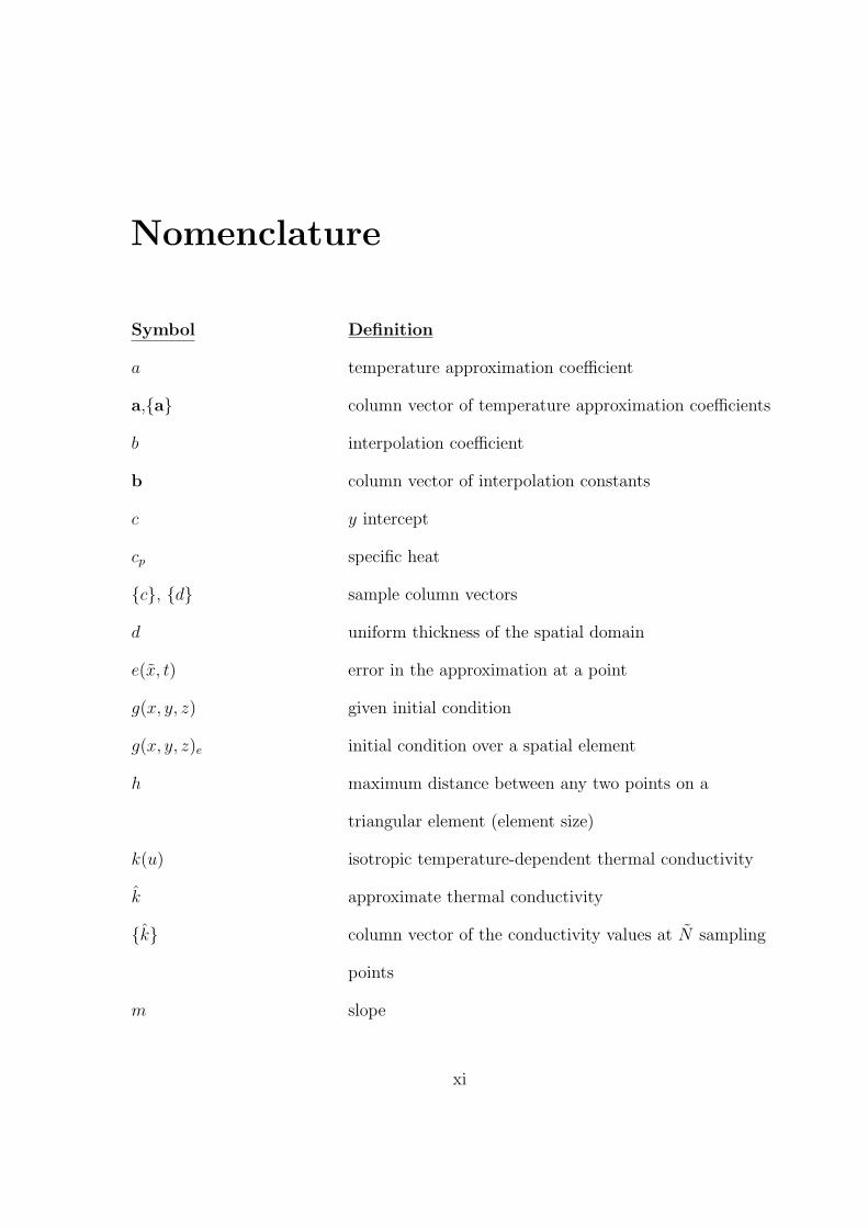
Nomenclature

Symbol Definition

a temperature approximation coefficient

a,a column vector of temperature approximation coefficients

b interpolation coefficient

b column vector of interpolation constants

c y intercept

cp specific heat

c, d sample column vectors

d uniform thickness of the spatial domain

e(x, t) error in the approximation at a point

g(x, y, z) given initial condition

g(x, y, z)e initial condition over a spatial element

h maximum distance between any two points on a

triangular element (element size)

k(u) isotropic temperature-dependent thermal conductivity

k approximate thermal conductivity

k column vector of the conductivity values at N sampling

points

m slope

xi

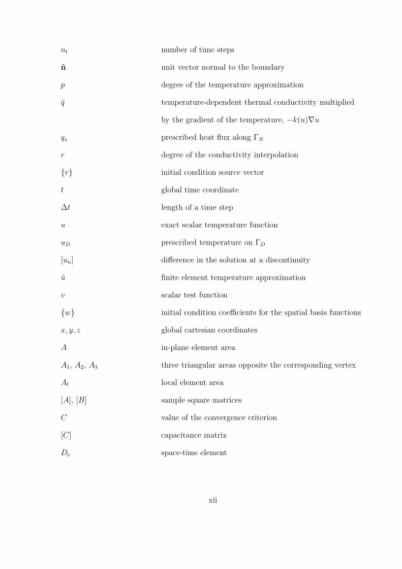
nt number of time steps

n unit vector normal to the boundary

p degree of the temperature approximation

q temperature-dependent thermal conductivity multiplied

by the gradient of the temperature, −k(u)∇u

qs prescribed heat flux along ΓN

r degree of the conductivity interpolation

r initial condition source vector

t global time coordinate

∆t length of a time step

u exact scalar temperature function

uD prescribed temperature on ΓD

[un] difference in the solution at a discontinuity

u finite element temperature approximation

v scalar test function

w initial condition coefficients for the spatial basis functions

x, y, z global cartesian coordinates

A in-plane element area

A1, A2, A3 three triangular areas opposite the corresponding vertex

Al local element area

[A], [B] sample square matrices

C value of the convergence criterion

[C] capacitance matrix

De space-time element

xii

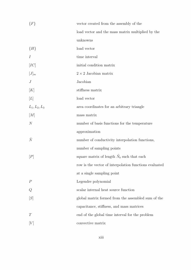
F vector created from the assembly of the

load vector and the mass matrix multiplied by the

unknowns

H load vector

I time interval

[IC] initial condition matrix

[J ]m 2× 2 Jacobian matrix

J Jacobian

[K] stiffness matrix

[L] load vector

L1, L2, L3 area coordinates for an arbitrary triangle

[M ] mass matrix

N number of basis functions for the temperature

approximation

N number of conductivity interpolation functions,

number of sampling points

[P ] square matrix of length Nb such that each

row is the vector of interpolation functions evaluated

at a single sampling point

P Legendre polynomial

Q scalar internal heat source function

[S] global matrix formed from the assembled sum of the

capacitance, stiffness, and mass matrices

T end of the global time interval for the problem

[V ] convective matrix

xiii

α, β local coordinates for the interior basis functions

η local coordinate for through-thickness basis

θ column vector of Nt time basis functions

θ column vector of Nt time interpolation functions

ξ local in-plane coordinate for an element

ρ density

τ local time coordinate

φ column vector of Nip in-plane basis functions

φ column vector of Nip in-plane interpolation functions

χ column vector of Nb element basis functions

χ column vector of Nb interpolation functions

ψ column vector of Ntk through-thickness basis functions

ψ column vector of Ntk through-thickness interpolation

functions

Γ total boundary of the global domain

ΓD, ΓN Dirichlet and Neumann boundaries

Υj jth global space-time basis function

Ω spatial domain

Norms Definition

‖ ‖H1(Ω) H1 norm in space at a point in time

‖ ‖L2(In,L2(Ω)) L2 norm over a single time step with an L2 norm in

space

‖ ‖L2(I,H1(Ω)) L2 norm over I with an H1 norm in space

xiv

Subscripts Definition

0 first time step

b total number on an element

e element

f finite number of terms

i, j, k, l, m indices

ip in-plane

n nth time step

t time

tk through-thickness

[ ]e element matrix

[ ]l local matrix

[ ]master master matrix

Superscripts Definition

+ beginning of a time step

− end of a time step

e edge

i interior

i, j, k indices

m iteration counter

sp sampling point

v vertex

T transpose

[ ]1,2,3,4 denote four different local matrices

xv

Operators Definition

∇ column vector gradient operator, [ ∂∂x

, ∂∂y

, ∂∂z

]T

⊗ outer tensor product

xvi

Chapter 1

Introduction

Hypersonic and reentry vehicles are exposed to high temperatures and large temperature

gradients as they travel through the atmosphere. Friction between the atmosphere and

the vehicle creates excessive heat that could result in significant damage or destruction

of the vehicle. The shuttle orbiter has a Thermal Protection System (TPS) designed to

protect it during reentry. The TPS on the orbiter consists of ceramic tiles, reinforced

carbon-carbon, and insulation blankets that protect the aluminum structure of the or-

biter from extreme heat. The next generation crew return vehicle (CRV) will also need

protection from the extreme heat of reentry. Future launch vehicle designs will likely use

non-insulated hot structures and multifunctional structures. Both hot and multifunc-

tional structures are designed to sustain thermal and aerodynamic loads simultaneously

unlike the separate TPS and aluminum structure used for the orbiter. The use of a sin-

gle structure to sustain thermal and aerodynamic loads can result in significant weight

savings. Accurate methods of performing thermal and structural analyses for multifunc-

tional and hot structures are needed.

The thermal response of a material can seriously impact its structural performance.

In order to determine accurately the effect of thermal stresses on the material, the tem-

perature distribution within the material must be determined. Finite element methods

are used to perform structural and thermal analyses. Commercial finite element codes,

1

such as NASTRAN [1] and ABAQUS [2], are capable of performing both thermal and

structural analyses. These codes rely on three-dimensional elements for the thermal anal-

ysis and two-dimensional elements for the structural analysis. In order to perform an

accurate analysis including thermal stress, separate meshes are created for the structural

and thermal analyses.

Conduction heat transfer problems are usually analyzed with traditional finite element

methods in space. In traditional, or h-version, finite elements the temperature approx-

imation is linear over an element. The solution is improved by increasing the number

of elements in the mesh until the solution achieves the required accuracy. This type of

refinement is computationally expensive since a new mesh must be created when the

number of elements is increased. Higher-degree spatial elements, or p-version elements,

increase the accuracy of the finite element method by allowing polynomial approxima-

tions of higher degree over an element. This allows a smaller number of elements to

capture the temperature distribution. The problem with traditional p-version (or La-

grange) elements is that as the degree of the polynomial approximation over an element

is increased, additional nodes must be added to each element. In addition to adding

new nodes, the basis functions change as the degree of the polynomial approximation is

increased. Hence, this method can become computationally expensive since a new mesh

must be created when nodes are added to the mesh and the basis functions are redefined.

Commercial finite element codes normally analyze transient problems of conduction

heat transfer using finite difference schemes in time. In order to provide an accurate

approximation in time, finite difference methods usually require the use of small time

steps. This often results in a large number of time steps, increasing the computational

expense of the analysis. Finite difference methods also impose limits on the size of the

time step needed for stability, with large time steps often resulting in unstable approxima-

2

tions. Finite difference methods become computationally expensive because the solution

is calculated at each time step and numerous time steps are required.

Another difficulty encountered in accurately approximating conduction heat transfer

is the variation in the thermal conductivity of a material with temperature. While

the thermal conductivity of a material can be approximated as a constant for small

temperature ranges, over large temperature ranges the thermal conductivity can vary

greatly. This variation in the thermal conductivity makes the problem nonlinear. In

order to obtain a solution, an iterative scheme must be used in combination with a

method to account for this variation in the thermal conductivity. Current methods used

to account for this variation assume that the thermal conductivity is constant over each

element or alternatively, the finite element integrals containing the thermal conductivity

are integrated using Gaussian quadrature. The first method requires numerous elements

in order to achieve an accurate approximation and the second requires a large number of

integration points for acceptable accuracy.

A hierarchical p-version space-time finite element method for nonlinear problems with

a structurally-compatible mesh would eliminate the weaknesses of traditional finite ele-

ment and finite difference methods. Hierarchical p-version finite elements allow higher

degrees of approximation on each element. Unlike traditional p-version elements, hier-

archical elements do not require additional nodes as the degree of the approximation is

increased. Instead, existing nodes acquire additional degrees of freedom as the degree

of the spatial approximation increases. This eliminates the need for new nodes to be

added to the mesh as the degree of spatial approximation is increased. Also unlike tradi-

tional p-version basis functions, hierarchical basis functions do not change as the degree

of approximation is increased. If solutions requiring higher-degrees of approximation are

needed, the additional basis functions can simply be added to the original set of basis

3

functions. Hierarchical modelling also allows a three-dimensional domain to be collapsed

onto a two-dimensional domain. Two-dimensional elements can then be used to create

a structurally-compatible finite element mesh that can also perform a three-dimensional

thermal analysis. This mesh consists of two-dimensional in-plane elements with an im-

plied through-thickness. The need for separate meshes for structural and thermal analysis

can be eliminated by using hierarchical modelling.

A p-version discontinuous Galerkin time-stepping method provides several advantages

over the finite difference schemes normally used in time. This finite element method is

more accurate than the traditional finite difference methods and allows the temperature

over a time step to be represented by higher-degrees of approximation in time. This can

greatly reduce the number of time steps necessary to represent accurately the temperature

evolution by allowing larger time steps. The unconditional stability of the discontinuous

Galerkin method eliminates concerns over the size of the time step.

To model the nonlinearity of the problem, the thermal conductivity is interpolated

and an iterative solver is implemented. Higher-degree interpolants can then be used

over each element to accurately capture the variation in the thermal conductivity. This

method does not rely on a large number of elements or numerous integration points to

obtain an accurate approximation.

1.1 Review of Previous Work

Since the development of hierarchical p-version finite elements by Babuska, Szabo, and

Peano in 1970’s and 1980’s, several authors have utilized their benefits to solve a variety

of heat transfer problems [3], [4]. Tamma and Saw developed an adaptive method for

two-dimensional thermal analysis using p-version hierarchical elements [5]. Gould used

these elements to approximate radiation heat transfer problems [6]. Hierarchical p-version

4

elements have also been utilized by Tomey [7], Lang [8], and Walker [9].

The discontinuous Galerkin method was developed in the 1970’s as a method to

discretize the neutron transport equation (see [10], [11], and references therein). Later

the method was adapted and applied to parabolic partial differential equations [12]. A-

priori error estimates for the discontinuous Galerkin method have been developed as well

[10], [11], [12]. Tomey applied the method to linear, transient heat conduction problems

[7].

Several methods of accounting for the variation in the thermal conductivity have

been developed. One method assumes that the thermal conductivity is constant over

an element. In another method, the finite element integrals containing the thermal

conductivity are integrated using Gaussian quadrature [3]. Walker developed a method

to interpolate the thermal conductivity for steady-state heat conduction problems using

higher-degree interpolants that reduces calculation time by using master matrices [9].

1.2 Purpose

The purpose of this research is to develop, implement, and test a finite element formu-

lation for nonlinear, transient conduction heat transfer. A hierarchical p-version finite

element method is used in space and the discontinuous Galerkin finite element method

is used in time. An approach for applying non-constant initial conditions is developed

to account for initial conditions that vary over the spatial domain. The variation in the

thermal conductivity of the material is captured using polynomial interpolants. Mas-

ter matrices are used to improve computational efficiency. Sample problems with exact

solutions are solved to validate the method and demonstrate error convergence.

5

1.3 Scope

The finite element formulation for nonlinear, transient conduction heat transfer is de-

veloped in Chapter 2. The initial boundary value problem is presented and the weak

form is derived. The finite element formulation includes the approximation using fi-

nite elements, discontinuous Galerkin time-stepping, the Galerkin method in space, the

temperature approximation, and temperature-dependent thermal conductivity. The el-

ement matrices resulting from the finite element formulation are then presented. The

time-stepping solution method for the nonlinear problem is discussed and a section on

applying initial and boundary conditions ends the chapter.

The basis functions used in the temperature approximation are discussed in Chapter

3. The basis functions for the time, through-thickness, and in-plane approximations are

defined. The properties and advantages of the basis functions are also discussed.

Chapter 4 provides a description of the method used to account for the variation in

the thermal conductivity. The functions used to interpolate the thermal conductivity in

the time, through-thickness, and in-plane dimensions are defined. The optimization of

sampling points and the calculation of the interpolation coefficients are then discussed.

The chapter closes by providing the convergence criterion used for the iterative solver.

The implementation of the finite element method using computer code is discussed in

Chapter 5. The master matrices and integration techniques are discussed. The method

of accounting for the boundary conditions in the computer code ends the chapter.

In Chapter 6 the method is validated. Error convergence is discussed and sample

problems are constructed to test the computer code. Results from the sample problems

and error convergence plots show the validity of the method.

The final chapter contains a summary of this research, the conclusions drawn, and

some suggestions for future work.

6

Chapter 2

Finite Element Method

The partial differential equation governing nonlinear, transient conduction heat transfer

is difficult to solve analytically. The partial differential equation is nonlinear because the

thermal conductivity varies as a function of temperature. The finite element method is

used to obtain an approximate solution to the nonlinear partial differential equation.

A finite element method for solving the nonlinear, transient conduction heat transfer

problem is discussed in this chapter. The method uses hierarchical p-version finite ele-

ment methods in space and time. The Galerkin finite element method is used in space

and a discontinuous Galerkin finite element method is used in time. To account for the

temperature-dependent thermal conductivity, interpolation is used along with fixed point

iteration. The notation presented here is based on the notation of Walker [9] and Tomey

[7].

2.1 Initial Boundary Value Problem

Using the principle of the conservation of energy, the governing partial differential equa-

tion for nonlinear, transient conduction heat transfer in a three-dimensional domain is

ρcp∂u

∂t−∇T (k(u)∇u) = Q (2.1)

7

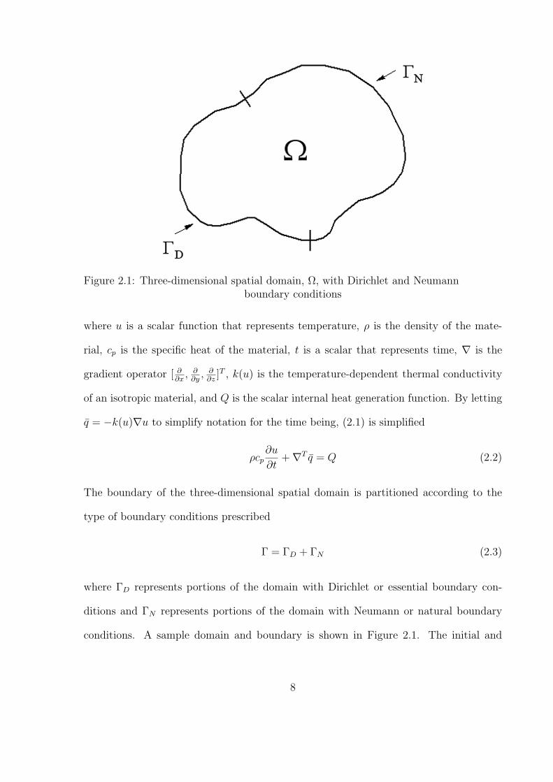
Figure 2.1: Three-dimensional spatial domain, Ω, with Dirichlet and Neumannboundary conditions

where u is a scalar function that represents temperature, ρ is the density of the mate-

rial, cp is the specific heat of the material, t is a scalar that represents time, ∇ is the

gradient operator [ ∂∂x

, ∂∂y

, ∂∂z

]T , k(u) is the temperature-dependent thermal conductivity

of an isotropic material, and Q is the scalar internal heat generation function. By letting

q = −k(u)∇u to simplify notation for the time being, (2.1) is simplified

ρcp∂u

∂t+∇T q = Q (2.2)

The boundary of the three-dimensional spatial domain is partitioned according to the

type of boundary conditions prescribed

Γ = ΓD + ΓN (2.3)

where ΓD represents portions of the domain with Dirichlet or essential boundary con-

ditions and ΓN represents portions of the domain with Neumann or natural boundary

conditions. A sample domain and boundary is shown in Figure 2.1. The initial and

8

boundary conditions for the partial differential equation are

u = uD on ΓD

−(k(u)∇u)T n = qs on ΓN

u(x, y, z, ti) = g(x, y, z) x, y, z ∈ Ω(2.4)

where n is a unit vector normal to the boundary, uD and qs are the specified temper-

ature and heat flux on the boundaries, and g(x, y, z) is a function that represents the

temperature distribution in the spatial domain, Ω, at some initial time, ti.

A solution to (2.1) is sought that satisfies the partial differential equation subject to

the given initial and boundary conditions.

2.2 Weak Formulation

To facilitate the development of the finite element method, the problem is cast into the

weak, or variational form. First (2.2) is multiplied by a test function, v. Next, the term

Qv is subtracted from both sides of the equation and the equation is integrated over the

the spatial domain, Ω, and the time interval of interest, (ti, T ], where without loss of

generality, ti is set equal to zero.

∫ T

0

∫

Ω

[ρcpv

∂u

∂t− v∇T q −Qv

]dΩ dt = 0 (2.5)

The test function can be any integrable function and is subject to less stringent regularity

requirements than the dependent variable, u. At this point in the formulation, this

weighted integral statement is equivalent to the partial differential equation and does not

include the boundary conditions [13].

The product rule and the divergence theorem are used to weaken the regularity re-

quirement on u and include the boundary conditions in the finite element formulation.

By the product rule

∫

Ωv∇T q dΩ =

∫

Ω∇T (qv)−

∫

Ω(∇v)T q dΩ (2.6)

9

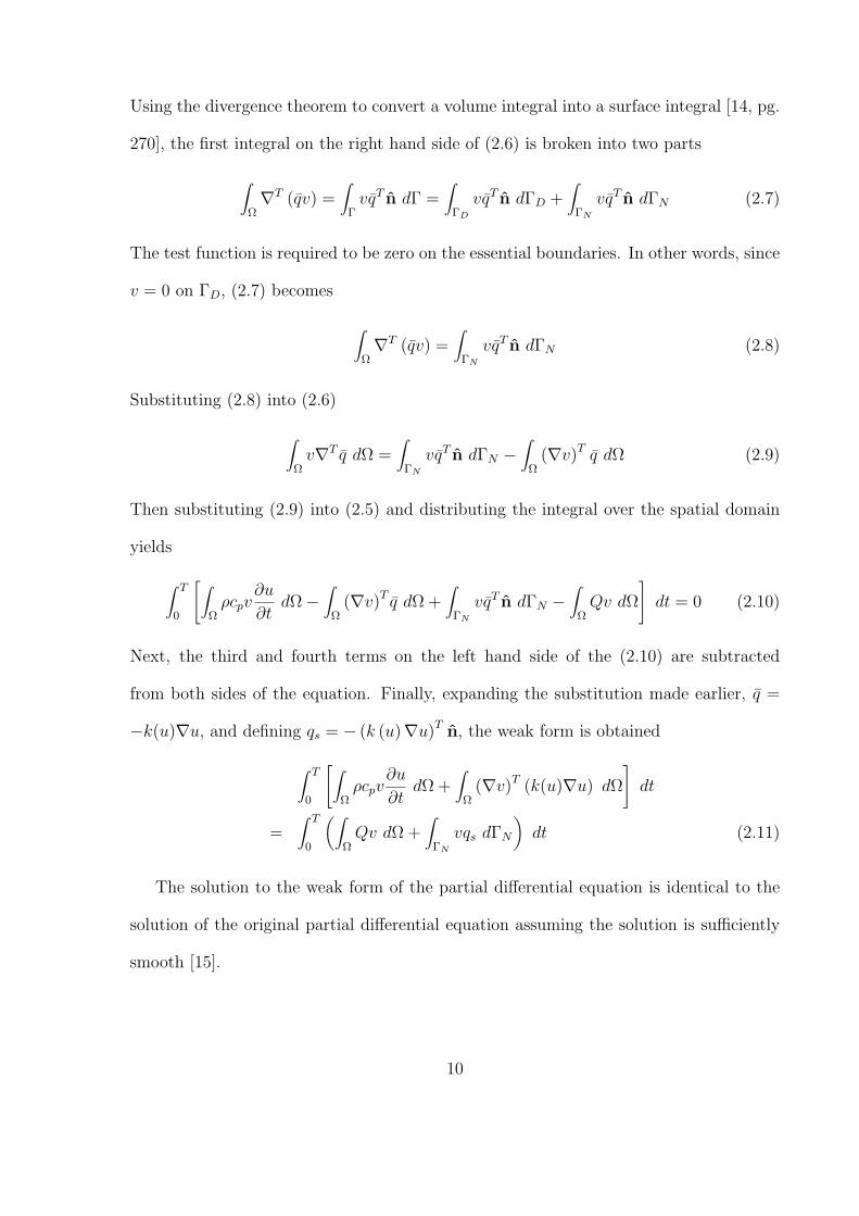
Using the divergence theorem to convert a volume integral into a surface integral [14, pg.

270], the first integral on the right hand side of (2.6) is broken into two parts

∫

Ω∇T (qv) =

∫

ΓvqT n dΓ =

∫

ΓD

vqT n dΓD +∫

ΓN

vqT n dΓN (2.7)

The test function is required to be zero on the essential boundaries. In other words, since

v = 0 on ΓD, (2.7) becomes

∫

Ω∇T (qv) =

∫

ΓN

vqT n dΓN (2.8)

Substituting (2.8) into (2.6)

∫

Ωv∇T q dΩ =

∫

ΓN

vqT n dΓN −∫

Ω(∇v)T q dΩ (2.9)

Then substituting (2.9) into (2.5) and distributing the integral over the spatial domain

yields

∫ T

0

[∫

Ωρcpv

∂u

∂tdΩ−

∫

Ω(∇v)T q dΩ +

∫

ΓN

vqT n dΓN −∫

ΩQv dΩ

]dt = 0 (2.10)

Next, the third and fourth terms on the left hand side of the (2.10) are subtracted

from both sides of the equation. Finally, expanding the substitution made earlier, q =

−k(u)∇u, and defining qs = − (k (u)∇u)T n, the weak form is obtained

∫ T

0

[∫

Ωρcpv

∂u

∂tdΩ +

∫

Ω(∇v)T (k(u)∇u) dΩ

]dt

=∫ T

0

(∫

ΩQv dΩ +

∫

ΓN

vqs dΓN

)dt (2.11)

The solution to the weak form of the partial differential equation is identical to the

solution of the original partial differential equation assuming the solution is sufficiently

smooth [15].

10

2.3 Finite Element Formulation

The weak form has a solution space that is infinite dimensional. The solution to the

weak form, u, can be expressed as an infinite series

u(x, y, z, t) =∞∑

j=1

Υj(x, y, z, t)aj (2.12)

where Υj are global basis functions defined over the space and time domain, Ω and (0, T ]

respectively, and aj are unknown constants. Since obtaining an exact solution to the

weak form of the problem is often difficult or impossible, the finite element method is

used to obtain an approximate solution, u. The approximate solution is a truncation of

the infinite series to a finite series with Nf terms

u(x, y, z, t) =Nf∑

j=1

Υj(x, y, z, t)aj (2.13)

A projection of the infinite dimensional solution space onto a finite dimensional solution

space is sought. This projection space is a subspace of the infinite dimensional solution

space.

In the finite element method, the domain is partitioned into elements. For the prob-

lems discussed in this research, space-time elements are used since the finite element

method is used in both space and time. The finite element mesh spans the entire spatial

and temporal domain of the problem. The mesh is created by partitioning the domain

into elements and the elements are assembled to create a global mesh.

In Figure 2.2, a sample space-time mesh for a one-dimensional transient problem is

shown. The nodes in the mesh are represented by the symbols • and ×. A space-time

element is denoted by De, where e is the number of the sample element. The element

D2 is represented in the global, element, and local contexts. In the element context, the

spatial component of D2 is denoted as Ωe and the time component of D2 is denoted by

11

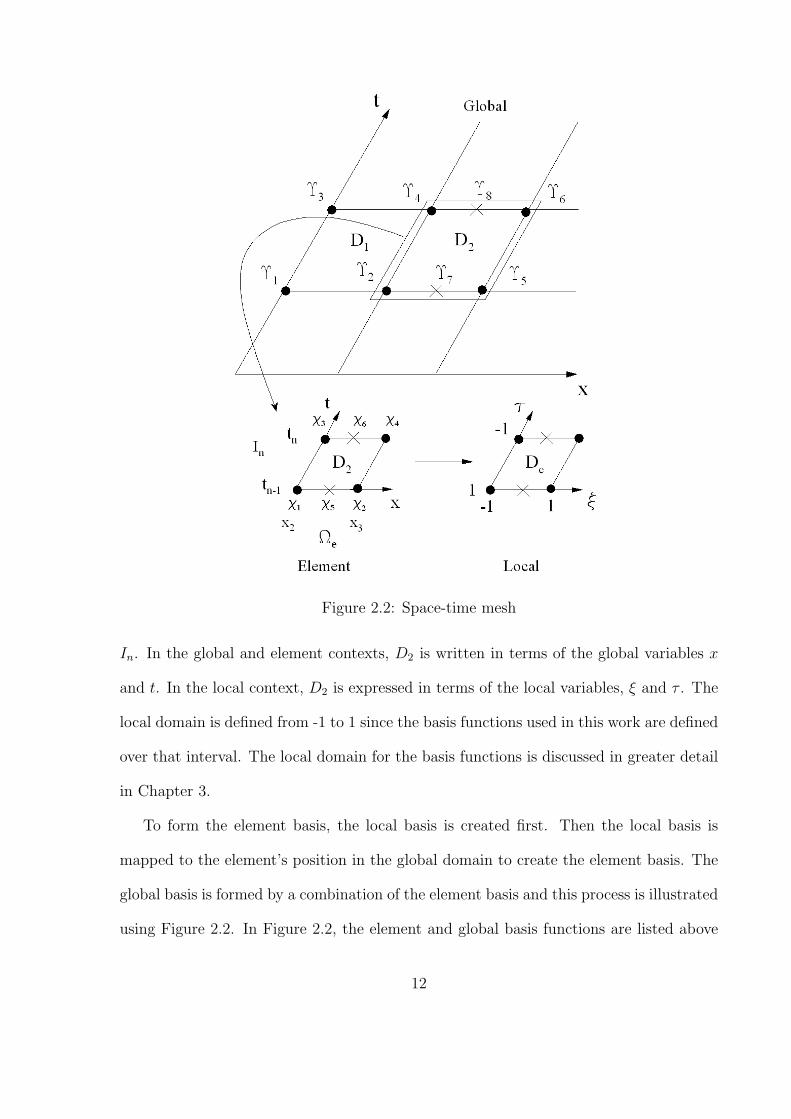
Figure 2.2: Space-time mesh

In. In the global and element contexts, D2 is written in terms of the global variables x

and t. In the local context, D2 is expressed in terms of the local variables, ξ and τ . The

local domain is defined from -1 to 1 since the basis functions used in this work are defined

over that interval. The local domain for the basis functions is discussed in greater detail

in Chapter 3.

To form the element basis, the local basis is created first. Then the local basis is

mapped to the element’s position in the global domain to create the element basis. The

global basis is formed by a combination of the element basis and this process is illustrated

using Figure 2.2. In Figure 2.2, the element and global basis functions are listed above

12

their corresponding nodes in the appropriate context. The element basis functions for

D1 are χ1, χ2, χ3, and χ4 and the global basis functions, in the same order, are given

above the global nodes in Figure 2.2. The global and local basis functions for D2 are

also shown. The global basis functions Υ1, Υ3, Υ5, Υ6, Υ7, and Υ8 are identical to the

element basis functions χ1, χ3, χ2, χ4, χ5, and χ6 respectively since these global basis

functions are not shared among the spatial elements. However, Υ2 is a combination of

the element basis functions χ2 from element one and χ1 from element two. Also, Υ4 is

a combination of the element basis functions χ4 from element one and χ3 from element

two.

The approximate solution over the time step tn−1 to tn and the entire spatial domain

is given by scaling each one of the global basis functions by the corresponding global

constant, aj, and summing. These global constants are calculated by solving the finite

element equations. The approximate solution over the time step tn−1 to tn for the sample

mesh shown in Figure 2.2 is

un = Υ1a1 + Υ2a2 + Υ3a3 + Υ4a4 + Υ5a5 + Υ6a6 + Υ7a7 + Υ8a8 (2.14)

The approximate solution can also be represented over each element in terms of the

element basis functions. The approximate solution for D2 over a single time step, un,2 is

given by multiplying each element basis function by the appropriate global constant and

summing

un,2 = χ1a2 + χ2a5 + χ3a4 + χ4a6 + χ5a7 + χ6a8 (2.15)

To represent two and three-dimensional spatial solutions using element basis func-

tions, the process is the same. The general approximate solution for any element over a

single time step, un,e, is expressed as

un,e =Nb∑

m=1

χm(Ω, t)am (2.16)

13

where χm are the element basis functions, Nb is the total number of basis functions for

that element, and am are the global constants associated with the global basis functions

that span the element. In a more compact notation

un,e = χTan,e (2.17)

where χT is a row vector of Nb element basis functions and an,e is a column vector of the

global constants for that space-time element.

2.3.1 Discontinuous Galerkin Method in Time

The global time domain is specified from time zero to some later time, T . To apply the

finite element method in time, the global time domain is partitioned into nt elements so

that the time interval of each time step is specified by In = [tn−1, tn]. Each time step has

a length of ∆t = tn − tn−1.

A major advantage of the discontinuous Galerkin method is that the method is uncon-

ditionally stable for linear parabolic problems [16]. This method allows for discontinuities

or jumps in the solution between the time steps. An example of a discontinuous solution

in time is shown in Figure 2.3. In Figure 2.3, the values of the solution at a discontinuity

are given by u−n and u+n such that

u−n = limε→0

u ( · , tn − ε)

u+n = lim

ε→0u ( · , tn + ε) (2.18)

These represent the values of the solution at some time tn for the left and right elements

respectively. The difference in the solution at a discontinuity is given by

[un] = u+n − u−n (2.19)

Since the exact solution is continuous in time, continuity should be enforced in some

way. Continuity is weakly enforced by multiplying the two temperature values at the

14

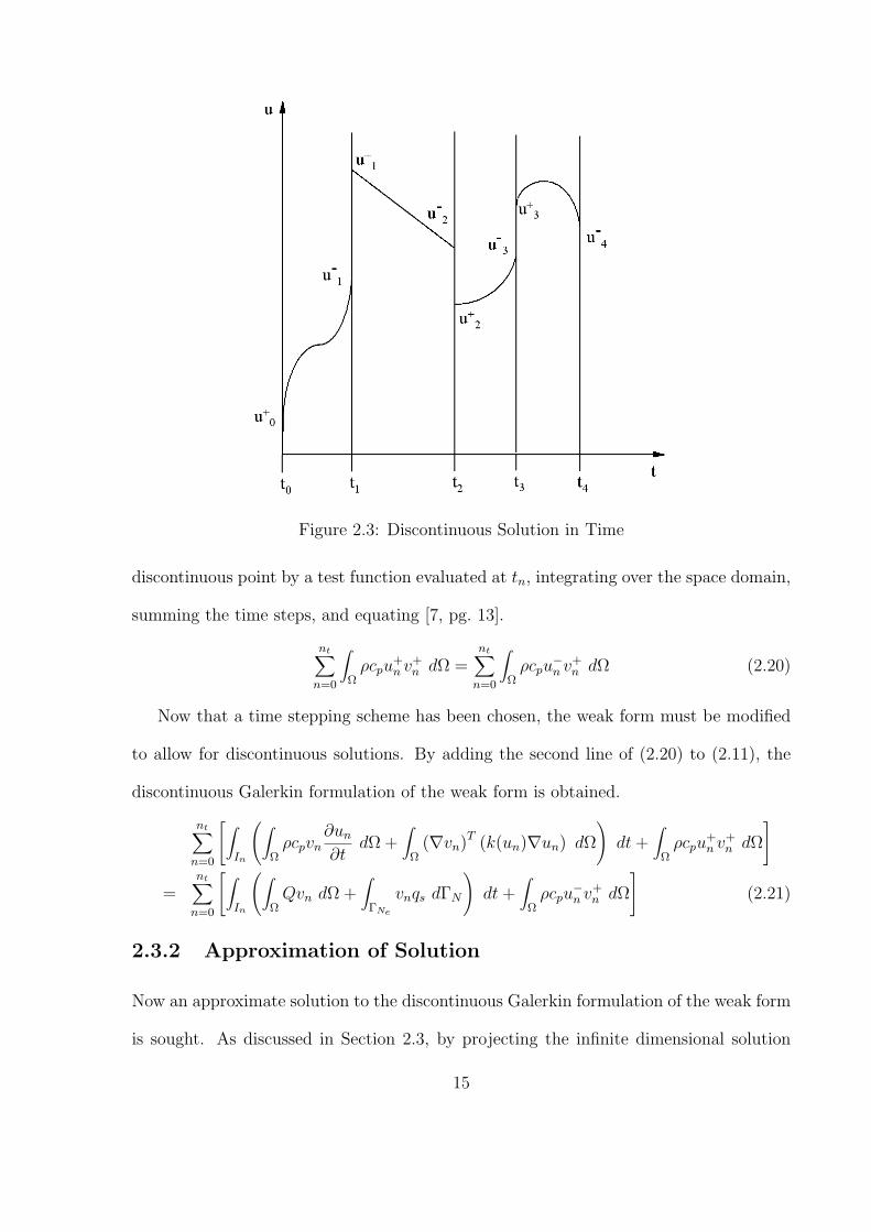
Figure 2.3: Discontinuous Solution in Time

discontinuous point by a test function evaluated at tn, integrating over the space domain,

summing the time steps, and equating [7, pg. 13].

nt∑

n=0

∫

Ωρcpu

+n v+

n dΩ =nt∑

n=0

∫

Ωρcpu

−n v+

n dΩ (2.20)

Now that a time stepping scheme has been chosen, the weak form must be modified

to allow for discontinuous solutions. By adding the second line of (2.20) to (2.11), the

discontinuous Galerkin formulation of the weak form is obtained.

nt∑

n=0

[∫

In

(∫

Ωρcpvn

∂un

∂tdΩ +

∫

Ω(∇vn)T (k(un)∇un) dΩ

)dt +

∫

Ωρcpu

+n v+

n dΩ

]

=nt∑

n=0

[∫

In

(∫

ΩQvn dΩ +

∫

ΓNe

vnqs dΓN

)dt +

∫

Ωρcpu

−n v+

n dΩ

](2.21)

2.3.2 Approximation of Solution

Now an approximate solution to the discontinuous Galerkin formulation of the weak form

is sought. As discussed in Section 2.3, by projecting the infinite dimensional solution

15

space to a finite dimensional subspace, an approximate solution to the discontinuous

Galerkin formulation of the weak form is obtained. The exact solution over a time step,

un, becomes un and the test function over a time step, vn, becomes vn such that un and

vn will represent functions from the subspaces of the exact solution space when summed

over all time steps. By approximating un and vn (2.21) becomes

nt∑

n=0

[∫

In

(∫

Ωρcpvn

∂un

∂tdΩ +

∫

Ω(∇vn)T (k(un)∇un) dΩ

)dt +

∫

Ωρcpu

+n v+

n dΩ

]

=nt∑

n=0

[∫

In

(∫

ΩQvn dΩ +

∫

ΓNe

vnqs dΓN

)dt +

∫

Ωρcpu

−n v+

n dΩ

](2.22)

The domain has been partitioned into space-time elements and in order to use the finite

element method, the individual elements must be assembled to form the global domain

in both space and time. The time domain has been broken into steps, but the spatial

domain still needs to be partitioned. This is done by summing over the total number

of elements at a particular time step, Ne. The approximate solution at a time step,

un, becomes un,e and the test function at a time step, vn, becomes vn,e such that un,e

and vn,e represent the approximate solution over a space-time element at a specific time

step. When these space-time elements are assembled, they form the entire spatial domain

over that time step. By summing over the space-time elements at each time step (2.22)

becomes

nt∑

n=0

Ne∑

e=1

[∫

In

(∫

Ωe

ρcpvn,e∂un,e

∂tdΩe +

∫

Ωe

(∇vn,e)T (ke(un,e)∇un,e) dΩe

)dt

+∫

Ωe

ρcpu+n,ev

+n,e dΩe

](2.23)

=nt∑

n=0

Ne∑

e=1

[∫

In

(∫

Ωe

Qvn,e dΩe +∫

ΓNe

vn,eqs dΓNe

)dt +

∫

Ωe

ρcpu−n,ev

+n,e dΩe

]

For an initial boundary value problem, an initial condition, u(x, y, z, ti) is given.

From this initial condition, the approximate temperature distribution over the mesh at

the left end of the first time step, u+0 , is known. Using this information, an explicit time

16

stepping scheme is used so that the temperature distribution for the current time step is

determined using the solution from the previous time step. Modifying (2.23) to reflect

time stepping and rearranging, the formulation for the time stepping scheme becomes

Ne∑

e=1

[∫

Ωe

(∫

In

[ρcpvn,e

∂un,e

∂t+ (∇vn,e)

T (ke(un,e)∇un,e)

]dt + ρcpu

+n,ev

+n,e

)dΩe

]

=Ne∑

e=1

[∫

Ωe

(∫

In

Qvn,e dt + ρcpu−n−1,ev

+n−1,e

)dΩe +

∫

ΓNe

∫

In

vn,eqs dt dΓNe

](2.24)

2.3.3 Temperature Approximation

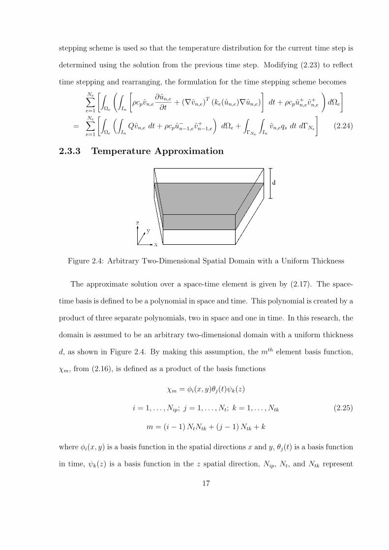
Figure 2.4: Arbitrary Two-Dimensional Spatial Domain with a Uniform Thickness

The approximate solution over a space-time element is given by (2.17). The space-

time basis is defined to be a polynomial in space and time. This polynomial is created by a

product of three separate polynomials, two in space and one in time. In this research, the

domain is assumed to be an arbitrary two-dimensional domain with a uniform thickness

d, as shown in Figure 2.4. By making this assumption, the mth element basis function,

χm, from (2.16), is defined as a product of the basis functions

χm = φi(x, y)θj(t)ψk(z)

i = 1, . . . , Nip; j = 1, . . . , Nt; k = 1, . . . , Ntk (2.25)

m = (i− 1) NtNtk + (j − 1) Ntk + k

where φi(x, y) is a basis function in the spatial directions x and y, θj(t) is a basis function

in time, ψk(z) is a basis function in the z spatial direction, Nip, Nt, and Ntk represent

17

the total number of basis functions in the in-plane (x-y), time, and through-thickness

directions respectively such that Nb = NipNtNtk. These polynomials are described in

greater detail in the next chapter. Then, χT is a row vector of all Nb basis functions

from (2.26). Using this definition for χT , the approximate solution over an element from

(2.17) becomes

un,e =Nip∑

i=1

Nt∑

j=1

Ntk∑

k=1

φi(x, y)θj(t)ψk(z)am (2.26)

This equation is written in a more elegant form using the outer tensor product operator,

⊗, and by writing φ, θ, and ψ as vectors. Also, note that the space-time dependence of

the basis functions is dropped from the notation for simplicity.

un,e = χTan,e = (φ⊗ θ ⊗ ψ)T an,e (2.27)

The Galerkin method is used in the spatial approximation so that the test function, vn,e

is defined using the same basis functions that were used for the approximate solution

vn,e = χm = φiθjψk (2.28)

where vn,e is a test function on an element for a single time step. By substituting every

basis function for the test function, a set of equations can be written and the test function,

vn,e, is replaced by a vector of the basis functions

vn,e = χ = (φ⊗ θ ⊗ ψ) (2.29)

The outer tensor product operator, ⊗, applies to matrices and vectors. Below a

sample is shown to illustrate how the operator is used. Given

[A] =

a11 a12 a13

a21 a22 a23

a31 a32 a33

[B] =

[b11 b12

b21 b22

]c =

c1

c2

d =

d1

d2

d3

18

then

[A]⊗ [B] =

a11b11 a11b12 a12b11 a12b12 a13b11 a13b12

a11b21 a11b22 a12b21 a12b22 a13b21 a13b22

a21b11 a21b12 a22b11 a22b12 a23b11 a23b12

a21b21 a21b22 a22b21 a22b22 a23b21 a23b22

a31b11 a31b12 a32b11 a32b12 a33b11 a33b12

a31b21 a31b22 a32b21 a32b22 a33b21 a33b22

and

c ⊗ d =

c1d1

c1d2

c1d3

c2d1

c2d2

c2d3

Now, substituting the first part from (2.27) and (2.29), and leaving the thermal

conductivity as a function of temperature, (2.24) is written as

Ne∑

e=1

[∫

Ωe

(∫

In

[ρcpχ

∂χT

∂tan,e + ke(un,e)

(∇χT

)T ∇χTan,e

]dt + ρcpχ

+(χ+

)Tan,e

)dΩe

]

=Ne∑

e=1

[∫

Ωe

(∫

In

Qχ dt + ρcpχ− (

χ+)T

an−1,e

)dΩe +

∫

ΓNe

∫

In

χqs dt dΓNe

](2.30)

The + and − superscripts denote evaluation of the basis functions at the beginning or

end of a time element, respectively. The element matrices and load vectors in (2.30) are

explicitly defined as

[Ce] =∫

Ωe

∫

In

ρcpχ∂χT

∂tdt dΩe

[Ke (un,e)] =∫

Ωe

∫

In

ke(un,e)(∇χT

)T ∇χT dt dΩe

[M++

e

]=

∫

Ωe

ρcpχ+

(χ+

)TdΩe (2.31)

[M−+

e

]=

∫

Ωe

ρcpχ− (

χ+)T

dΩe

He =∫

Ωe

∫

In

Qχ dt dΩe +∫

ΓNe

∫

In

χqs dt dΓNe

where [Ce] represents the element capacitance matrix, [Ke(un,e)] represents the element

stiffness (conductance) matrix, [M++e ] and [M−+

e ] are element mass matrices, and He

19

is the element load vector. Using the matrix and vector notation from (2.31), (2.30) can

be written as

Ne∑

e=1

[[Ce] + [Ke (un,e)] + [M++

e ]]an,e =

Ne∑

e=1

He+ [M−+e ] an−1,e (2.32)

These element matrices and vectors are assembled to form a global system of equations

that is solved at each time step. This assembly of element equations is denoted by the

summation over the elements. By using the explicit time stepping scheme, (2.32) is solved

nt times, once for each time step.

2.3.4 Temperature-Dependent Thermal Conductivity

The temperature dependence of the thermal conductivity must be taken into account in

the finite element formulation. The approximate temperature is defined by multiplying

each basis function by the appropriate unknown and summing. Each basis function is a

function of the spatial dimensions and time. This means that the thermal conductivity

is implicitly a function of the spatial dimensions, time, and the unknowns, an,e. To

approximate the thermal conductivity as a function of temperature, ke is defined over an

element

ke(un,e) ≈ ke =Nip∑

i=1

Nt∑

j=1

Ntk∑

k=1

φiθjψkbijk = χTbn,e =(φ⊗ θ ⊗ ψ

)Tbn,e (2.33)

where φ, θ, ψ are vectors that represent the interpolation functions over the in-plane,

time, and through-thickness dimensions respectively, Nip, Nt, and Ntk are the number of

interpolation functions in the in-plane, time, and through-thickness dimensions, and bn,e

is a vector of interpolation constants that is calculated from an,e. There are a total of Nb

interpolation functions such that

Nb = NipNtNtk (2.34)

20

The interpolation functions and the determination of the interpolation constants, bn,e,

are discussed in Chapter 4. Substituting (2.33) into [Ke (u (an,e))] in (2.31) gives

[Ke (an,e)] =∫

Ωe

∫

In

χTbn,e

(∇χT

)T ∇χT dt dΩe (2.35)

The stiffness matrix is no longer a function of the approximate temperature, rather it

is now a function of the unknowns. By taking this new representation of the stiffness

matrix into account, (2.32) becomes

Ne∑

e=1

[[Ce] + [Ke (an,e)] + [M++

e ]]an,e =

Ne∑

e=1

He+ [M−+e ] an−1,e (2.36)

2.4 Element Matrices

The element matrices as defined in (2.31) are inefficient for computational purposes. To

make calculation of these matrices more efficient, some modification is required. First, the

matrices and vectors without thermal conductivity will be modified. These matrices do

not contain interpolation functions or interpolation constants. The definition of χ from

(2.27) is inserted into (2.31) and the integral over the spatial domain is expanded into

separate integrals for the x− y plane (or in-plane), denoted by A (the area of an element

in the x − y plane), and z (or through-thickness) direction. Finally, the temperature

approximation basis functions are rearranged using the properties of the outer tensor

product and the constants are placed outside the integrals. Then, [Ce] is written as

[Ce] =∫

Ωe

∫

In

ρcpχ∂χT

∂tdt dΩe

=∫

A

∫ d2

− d2

∫ tn

tn−1

ρcp (φ⊗ θ ⊗ ψ)

(φ⊗ dθ

dt⊗ ψ

)T

dt dz dA (2.37)

= ρcp

∫

AφφT dA⊗

∫ tn

tn−1

θdθ

dt

T

dt⊗∫ d

2

− d2

ψψT dz

21

Now, [M++e ] is

[M++

e

]=

∫

Ωe

ρcpχ+

(χ+

)TdΩe

=∫

A

∫ d2

− d2

ρcp

(φ⊗ θ+ ⊗ ψ

) (φ⊗ θ+ ⊗ ψ

)Tdz dA (2.38)

= ρcp

∫

AφφT dA⊗ θ+

(θ+

)T ⊗∫ d

2

− d2

ψψT dz

Similarly, [M−+e ] becomes

[M−+

e

]=

∫

Ωe

ρcpχ− (

χ+)T

dΩe

=∫

A

∫ d2

− d2

ρcp

(φ⊗ θ− ⊗ ψ

) (φ⊗ θ+ ⊗ ψ

)Tdz dA (2.39)

= ρcp

∫

AφφT dA⊗ θ−

(θ+

)T ⊗∫ d

2

− d2

ψψT dz

Then, He is written as

He =∫

Ωe

∫

In

Qχ dt dΩe +∫

ΓNe

∫

In

χqs dt dΓNe

=∫

A

∫ d2

− d2

∫ tn

tn−1

Q (φ⊗ θ ⊗ ψ) dt dz dA (2.40)

+∫

ΓNe

∫ tn

tn−1

(φ⊗ θ ⊗ ψ) qs dt dΓNe

To simplify [Ke (an,e)], a few steps must be added to account for the thermal conduc-

tivity as a function of temperature. Starting from (2.35), the definitions of χ and χ are

inserted from (2.27) and (2.33) and the integral over the spatial domain is expanded into

separate integrals for the x− y plane and z direction.

[Ke (an,e)] =∫

A

∫ d2

− d2

∫ tn

tn−1

(φ⊗ θ ⊗ ψ

)Tbn,e

(∇ (φ⊗ θ ⊗ ψ)T

)T ∇ (φ⊗ θ ⊗ ψ)T dt dz dA

Next, the thermal conductivity interpolation is written as a sum and the interpolation

constant is placed outside the integrals.

[Ke (an,e)] =Nb∑

m=1

bm

∫

A

∫ d2

− d2

∫ tn

tn−1

φiθjψk

(∇ (φ⊗ θ ⊗ ψ)T

)T ∇ (φ⊗ θ ⊗ ψ)T dt dz dA

22

The single summation represents the three part summation in (2.33). The index for bm

is given by

m = (i− 1)NtNtk + (j − 1)Ntk + k (2.41)

such that bm is the mth interpolation constant on that element. Each piece of the sum-

mation represents one part of the stiffness matrix. Then, by considering one piece of the

summation and distributing the ∇ operator

[Ke (an,e)]m = bm

∫

A

∫ d2

− d2

∫ tn

tn−1

φiθjψk

[(∂φ

∂x⊗ θ ⊗ ψ

) (∂φ

∂x

T

⊗ θT ⊗ ψT

)+

(∂φ

∂y⊗ θ ⊗ ψ

) (∂φ

∂y

T

⊗ θT ⊗ ψT

)+

(φ⊗ θ ⊗ dφ

dz

) (φT ⊗ θT ⊗ dφ

dz

T)]

dt dz dA

where the m in [Ke (an,e)]m represents a single matrix in the summation over all of the

matrices generated by the different interpolation functions and constants. In other words

[Ke (an,e)] =Nb∑

m=1

[Ke (an,e)]m (2.42)

The temperature approximation basis functions are rearranged using the properties of

the tensor product and the gradient operator. The final form of the mth part of the

stiffness matrix is given by

[Ke (an,e)]m = bm

[∫

Aφi

[∂φ

∂x

∂φ

∂x

T

+∂φ

∂y

∂φ

∂y

T]

dA⊗∫ tn

tn−1

θjθθT dt⊗

∫ d2

− d2

ψkψψT dz

+∫

AφiφφT dA⊗

∫ tn

tn−1

θjθθT dt⊗

∫ d2

− d2

ψkdψ

dz

dψ

dz

T

dz

](2.43)

The stiffness matrix is given by

[Ke (an,e)] =Nb∑

m=1

bm

[∫

Aφi

[∂φ

∂x

∂φ

∂x

T

+∂φ

∂y

∂φ

∂y

T]

dA⊗∫ tn

tn−1

θjθθT dt⊗

∫ d2

− d2

ψkψψT dz

+∫

AφiφφT dA⊗

∫ tn

tn−1

θjθθT dt⊗

∫ d2

− d2

ψkdψ

dz

dψ

dz

T

dz

](2.44)

23

2.5 Time-Stepping Solution Method

The global system of equations given in (2.36),

Ne∑

e=1

[[Ce] + [Ke (an,e)] + [M++

e ]]an,e =

Ne∑

e=1

He+ [M−+e ] an−1,e

can be written as

[S (an)] an = Fn−1 (2.45)

where [S (an)] is the global matrix formed from the sum of the three matrices on the left

hand side, an is the global vector of unknowns, and Fn−1 is the vector on the right

hand side. The n and n − 1 subscripts denote the time step, such that n is the current

time step and n − 1 is the previous time step. Since the stiffness matrix, [Ke (an,e)], in

(2.45) is a function of the unknowns, the system of equations is nonlinear and must be

solved iteratively. The fixed point method is used in this research [17].

In the fixed point iteration method, an initial guess is made for the values of the

global unknowns. Since the problem considered in this work is transient, the solution

from the previous time step is used as the initial guess. For the first time step, the initial

condition is used. A flowchart for the time-stepping solution method including the fixed

point iteration is shown in Figure 2.5. The time-stepping solution method depicted in

Figure 2.5 is described in the following paragraphs.

Starting from the initial condition, the values of the global unknowns are calculated

and are specified by a0. The method for determining a0 from the initial condition is

discussed in the next section. Once a0 is known, the interpolation constants, bn,e, can be

calculated. Now that the interpolation constants are known, [S (a0)] can be formulated.

The iteration counter is denoted by m and the first step in the problem is written as

[S (a0)] am1 = F0 (2.46)

24

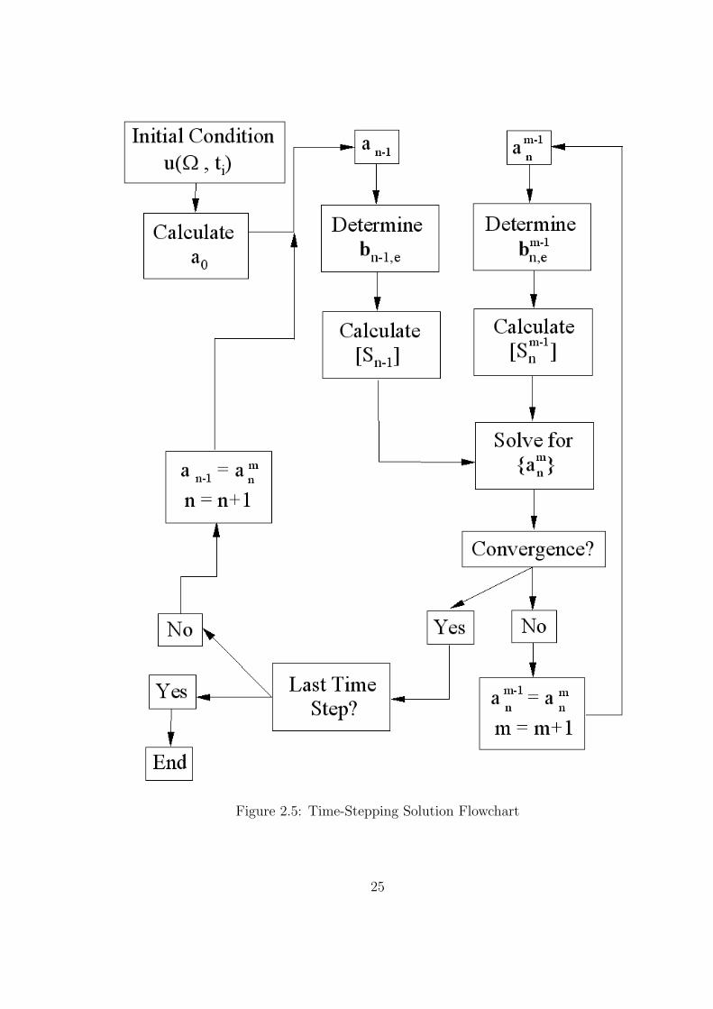
Figure 2.5: Time-Stepping Solution Flowchart

25

and is solved for the unknowns am1 . Now that am

1 is known, the iteration counter, m

is increased and these values are used to recalculate bn,e and [S]. Now the problem is

written as[S

(am−1

1

)]am

1 = F0 (2.47)

This equation is solved iteratively and bn,e and [S] are updated using the new unknowns

each time until the method converges. The right hand side of the problem does not

change with each iteration. If the difference, in some quantified manner, between am

and am−1 is less than a specified tolerance, then the iteration has converged and the final

solution at the time step, an, has been determined.

After the iteration converges, the time step counter, n, is increased to begin the next

time step and the solution that was just found is now written as an−1. The problem is

now cast as

[S (an−1)] amn = Fn−1 (2.48)

Again, this equation is solved for the unknowns and becomes

[S

(am−1

n

)]am

n = Fn−1 (2.49)

Then the problem is solved iteratively as before and [S] is updated using the previous

iterate until convergence is attained. The time step counter is then updated and the

method repeats from (2.48) for the next time step. This process is repeated until the

unknowns for the final time step have been determined.

2.6 Applying Initial and Boundary Conditions

The initial and boundary conditions for the problem are given by (2.4). Before (2.46),

(2.47), (2.48), and (2.49) are solved for the unknowns, the Dirichlet boundary conditions

must be enforced. For these boundary conditions, the temperature is specified on the

26

boundary and the values of the global unknowns are known. To enforce these boundary

conditions, the penalty method is used. This method is described in detail in Chapter

5. The Neumann boundary conditions are included in the element load vector He from

(2.40). For the Neumann boundary conditions, qs is specified and these values are used

in the calculation of the element load vector. The heat flux function, qs, is contained

in the second term on the right hand side of (2.40). The computer implementation for

these boundary conditions is also discussed in Chapter 5.

To start the time-stepping solution method described, the initial condition vector, a0,

must be determined. If the initial condition is a constant, then the linear spatial degrees

of freedom are set to the constant temperature specified by the initial condition and all

other degrees of freedom are set to zero. Occasionally, the initial condition, g(x, y, z), is

specified as a function of the spatial domain. In this case, a0 must be determined using

the basis functions. In order to find a0, an approximation of the initial condition, u0 is

sought such that∫

Ωv0u0 dΩ =

∫

Ωv0 g(x, y, z) dΩ (2.50)

By substituting (2.27) and (2.29) into (2.50)

∫

Ωχ0χ

T0 a0 dΩ =

∫

Ωχ0 g(x, y, z) dΩ (2.51)

Then by defining

[IC] =∫

Ωχ0χ

T0 dΩ (2.52)

r =∫

Ωχ0 g(x, y, z) dΩ (2.53)

and moving the constant vector a0 outside the integral, (2.51) is written as

[IC] a0 = r (2.54)

27

The global matrix, [IC], and the global vector r from (2.54) are created by forming

the element matrices and assembling

[IC]e =∫

AφφT dA⊗

∫ d2

− d2

ψψT dz (2.55)

[IC] =Ne∑

e=1

[IC]e (2.56)

re =∫

A

∫ d2

− d2

g(x, y, z)e (φ⊗ ψ) dA dz (2.57)

r =Ne∑

e=1

re (2.58)

where g(x, y, z)e represents the initial condition restricted to an element. These matrices

do not contain the time basis, θ, since the initial condition does not vary over time. They

also do not contain the interpolation for the thermal conductivity since the temperature

distribution has been explicitly defined by the initial condition.

Since the time basis is not used to create the matrices and vectors in (2.55) and (2.57),

(2.54) is rewritten without the time basis and solved for w, where w is a vector of

the coefficients that are multiplied by the appropriate basis functions to approximate the

initial condition

[IC] w = r (2.59)

The vector w will have a length of NipNtk since the time basis was not included. To

create a0 from w, the degrees of freedom used by the time basis must be included to

ensure that a0 is the appropriate size. The time basis must be modified since there is no

variation over time for the initial condition. To accomplish this, the constant time basis

functions are set equal to one and all other time basis functions are set equal to zero.

The degrees of freedom must be arranged in the appropriate order so that the order used

earlier, (φ⊗ θ ⊗ ψ), is followed. Finally, a0 is created by multiplying the values of w by

the modified time basis functions and by tracking the order of the degrees of freedom.

28

Chapter 3

Basis Functions

The basis functions and the necessary mapping relationships to convert from a local

element to a specific element in the global context are discussed in this chapter. The

functions used in this research were chosen because of their desirable numerical properties

and the ability to generalize the formulation of the local matrices.

3.1 Time Basis Functions

The time basis functions used in this work are the set of Legendre polynomials, Pn, that

can be generated using a recurrence relation [18, pg. 208]

Pn+1(τ) =(2n + 1) τPn(τ)− nPn−1(τ)

n + 1(3.1)

where P0(τ) = 1 and P1(τ) = τ . The first few Legendre polynomials are

P0(τ) = 1

P1(τ) = τ

P2(τ) =1

2

(3τ 2 − 1

)(3.2)

P3(τ) =1

2

(5τ 3 − 3τ

)

P4(τ) =1

8

(35τ 4 − 30τ 2 + 3

)

29

The time basis functions first introduced in (2.26) are defined as

θj(τ) = Pj(τ) for j = 0, . . . , pt (3.3)

where pt is the degree of the polynomial approximation in time. For an approximation

of degree pt, there are Nt time basis functions where Nt = pt + 1.

The Legendre polynomial basis presented here has advantages over the monomial

basis used by Tomey [7, pg. 20-2]. The Legendre polynomials are orthogonal over the

interval (−1, 1) resulting in element matrices that are less susceptible to computer round

off error. Matrix conditioning problems that occur when a monomial basis is used are

eliminated by using an orthogonal basis.

By taking into account the relationship between t and τ , a mapping can be established

to create the specific global time element from the local time element

t = tn−1 +∆t

2(τ + 1) (3.4)

τ =2

∆t(t− tn−1)− 1 (3.5)

where t is the time, tn−1 is the time at the left end of the time element, ∆t is the length

of the time element in the global context, ∆t = tn− tn−1, and τ is the local variable. By

differentiating (3.4) and rearranging

dt =∆t

2dτ (3.6)

dτ

dt=

2

∆t(3.7)

and by using the chain rule

d

dt=

d

dτ

dτ

dt=

2

∆t

d

dτ(3.8)

yields the necessary relationships for mapping from the local time element to the specific

global time element.

30

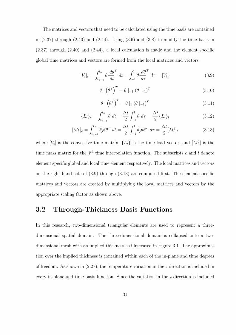
The matrices and vectors that need to be calculated using the time basis are contained

in (2.37) through (2.40) and (2.44). Using (3.6) and (3.8) to modify the time basis in

(2.37) through (2.40) and (2.44), a local calculation is made and the element specific

global time matrices and vectors are formed from the local matrices and vectors

[Vt]e =∫ tn

tn−1

θdθ

dt

T

dt =∫ 1

−1θ

dθ

dτ

T

dτ = [Vt]l (3.9)

θ+(θ+

)T= θ |−1 (θ |−1)

T (3.10)

θ−(θ+

)T= θ |1 (θ |−1)

T (3.11)

Lte =∫ tn

tn−1

θ dt =∆t

2

∫ 1

−1θ dτ =

∆t

2Ltl (3.12)

[M jt ]e =

∫ tn

tn−1

θjθθT dt =

∆t

2

∫ 1

−1θjθθ

T dτ =∆t

2[M j

t ]l (3.13)

where [Vt] is the convective time matrix, Lt is the time load vector, and [M jt ] is the

time mass matrix for the jth time interpolation function. The subscripts e and l denote

element specific global and local time element respectively. The local matrices and vectors

on the right hand side of (3.9) through (3.13) are computed first. The element specific

matrices and vectors are created by multiplying the local matrices and vectors by the

appropriate scaling factor as shown above.

3.2 Through-Thickness Basis Functions

In this research, two-dimensional triangular elements are used to represent a three-

dimensional spatial domain. The three-dimensional domain is collapsed onto a two-

dimensional mesh with an implied thickness as illustrated in Figure 3.1. The approxima-

tion over the implied thickness is contained within each of the in-plane and time degrees

of freedom. As shown in (2.27), the temperature variation in the z direction is included in

every in-plane and time basis function. Since the variation in the z direction is included

31

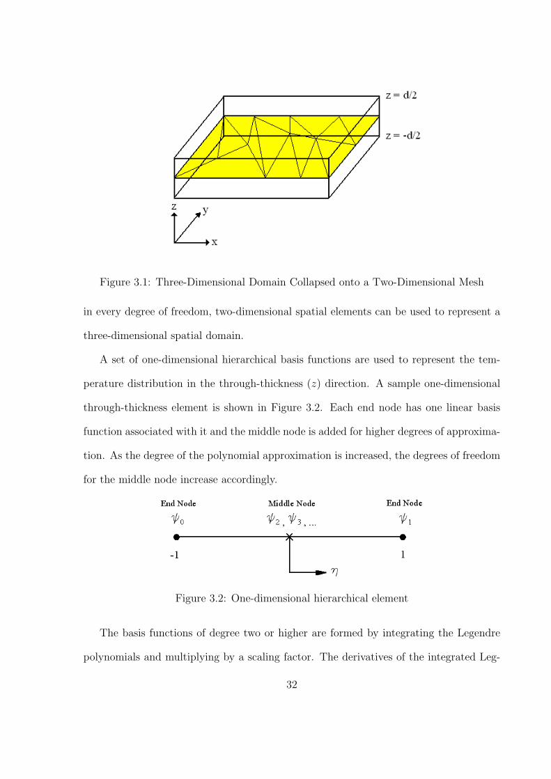
Figure 3.1: Three-Dimensional Domain Collapsed onto a Two-Dimensional Mesh

in every degree of freedom, two-dimensional spatial elements can be used to represent a

three-dimensional spatial domain.

A set of one-dimensional hierarchical basis functions are used to represent the tem-

perature distribution in the through-thickness (z) direction. A sample one-dimensional

through-thickness element is shown in Figure 3.2. Each end node has one linear basis

function associated with it and the middle node is added for higher degrees of approxima-

tion. As the degree of the polynomial approximation is increased, the degrees of freedom

for the middle node increase accordingly.

Figure 3.2: One-dimensional hierarchical element

The basis functions of degree two or higher are formed by integrating the Legendre

polynomials and multiplying by a scaling factor. The derivatives of the integrated Leg-

32

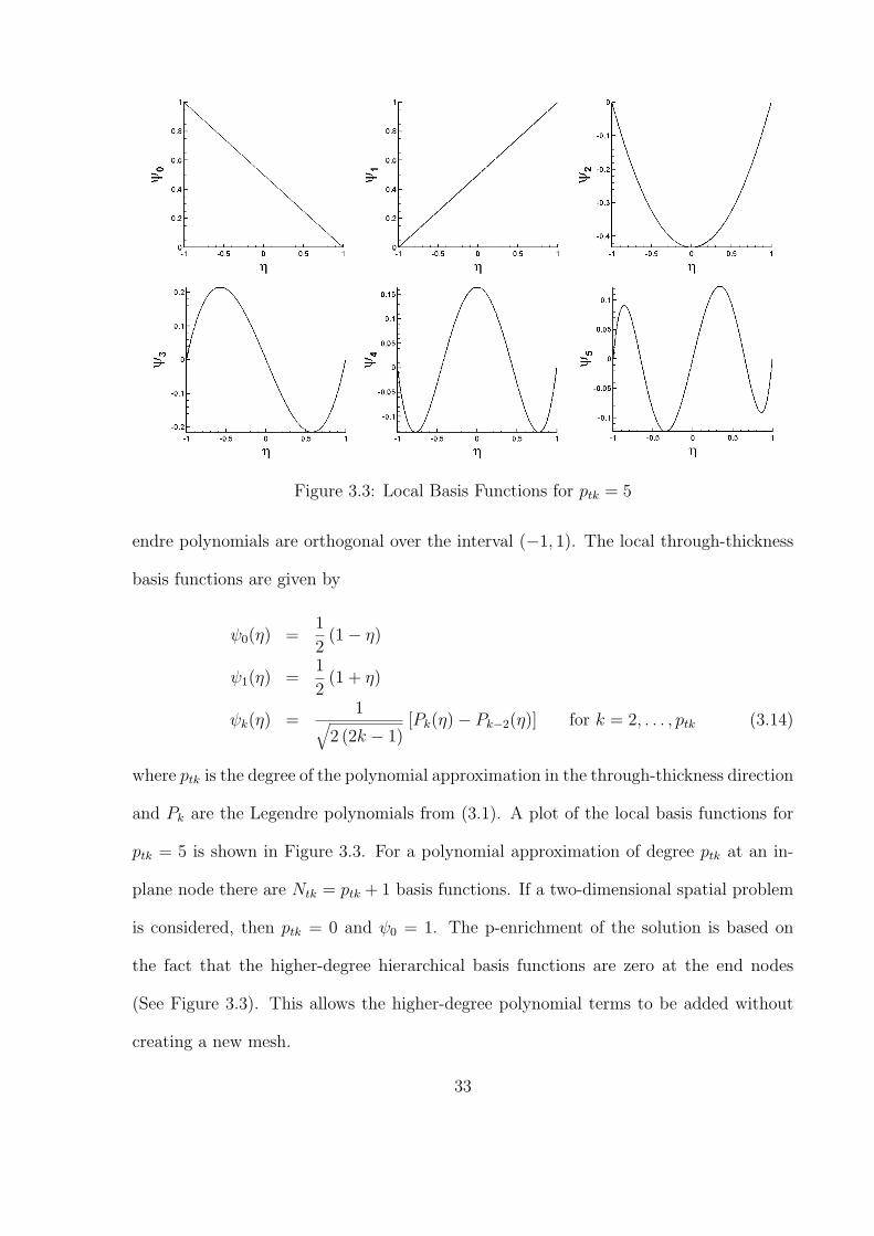
Figure 3.3: Local Basis Functions for ptk = 5

endre polynomials are orthogonal over the interval (−1, 1). The local through-thickness

basis functions are given by

ψ0(η) =1

2(1− η)

ψ1(η) =1

2(1 + η)

ψk(η) =1√

2 (2k − 1)[Pk(η)− Pk−2(η)] for k = 2, . . . , ptk (3.14)

where ptk is the degree of the polynomial approximation in the through-thickness direction

and Pk are the Legendre polynomials from (3.1). A plot of the local basis functions for

ptk = 5 is shown in Figure 3.3. For a polynomial approximation of degree ptk at an in-

plane node there are Ntk = ptk + 1 basis functions. If a two-dimensional spatial problem

is considered, then ptk = 0 and ψ0 = 1. The p-enrichment of the solution is based on

the fact that the higher-degree hierarchical basis functions are zero at the end nodes

(See Figure 3.3). This allows the higher-degree polynomial terms to be added without

creating a new mesh.

33

The global domain in the z-direction is −d2≤ z ≤ d

2. The local basis is used to create

the element specific basis by utilizing the relationships between the local coordinate, η,

and the global coordinate, z

η =2

dz (3.15)

z =d

2η (3.16)

By differentiating (3.16) and rearranging

dz =d

2dη (3.17)

dη

dz=

2

d(3.18)

and by applying the chain rule

d

dz=

d

dη

dη

dz=

2

d

d

dη(3.19)

the necessary relationships for mapping from the local through-thickness element to the

specific through-thickness element in the global domain are obtained. The matrices

and vectors that need to be calculated using the through-thickness basis are contained

in (2.37) through (2.40) and (2.44). Using (3.17) and (3.19) to modify the through-

thickness basis in (2.37) through (2.40) and (2.44), a local calculation is made and the

element specific matrices and vectors are formed from the local matrices and vectors

[Mtk]e =∫ d

2

− d2

ψψT dz =d

2

∫ 1

−1ψψT dη =

d

2[Mtk]l (3.20)

Ltke =∫ d

2

− d2

ψ dz =d

2

∫ 1

−1ψ dη =

d

2Ltkl (3.21)

[Mktk]e =

∫ d2

− d2

ψkψψT dz =d

2

∫ 1

−1ψkψψT dη =

d

2[Mk

tk]l (3.22)

[Kktk]e =

∫ d2

− d2

ψkdψ

dz

dψ

dz

T

dz =2

d

∫ 1

−1ψk

dψ

dη

dψ

dη

T

dη =2

d[Kk

tk]l (3.23)

34

where [Mtk] is the through-thickness mass matrix, Ltk is the through-thickness load

vector, and [Mktk] and [Kk

tk] are the through-thickness mass and stiffness matrices for

the kth through-thickness interpolation function. The subscripts e and l denote element

specific and local respectively. Again, the local matrices and vectors on the right hand side

are computed first. The element specific matrices and vectors are created by multiplying

the local matrices and vectors by the appropriate scaling factor.

3.3 Hierarchical In-Plane Basis Functions

In this research, two-dimensional triangular elements are used in the x − y or in-plane

directions. These triangular elements are hierarchical to allow the p-enrichment of the

approximation without mesh refinement. A sample triangular hierarchical element is

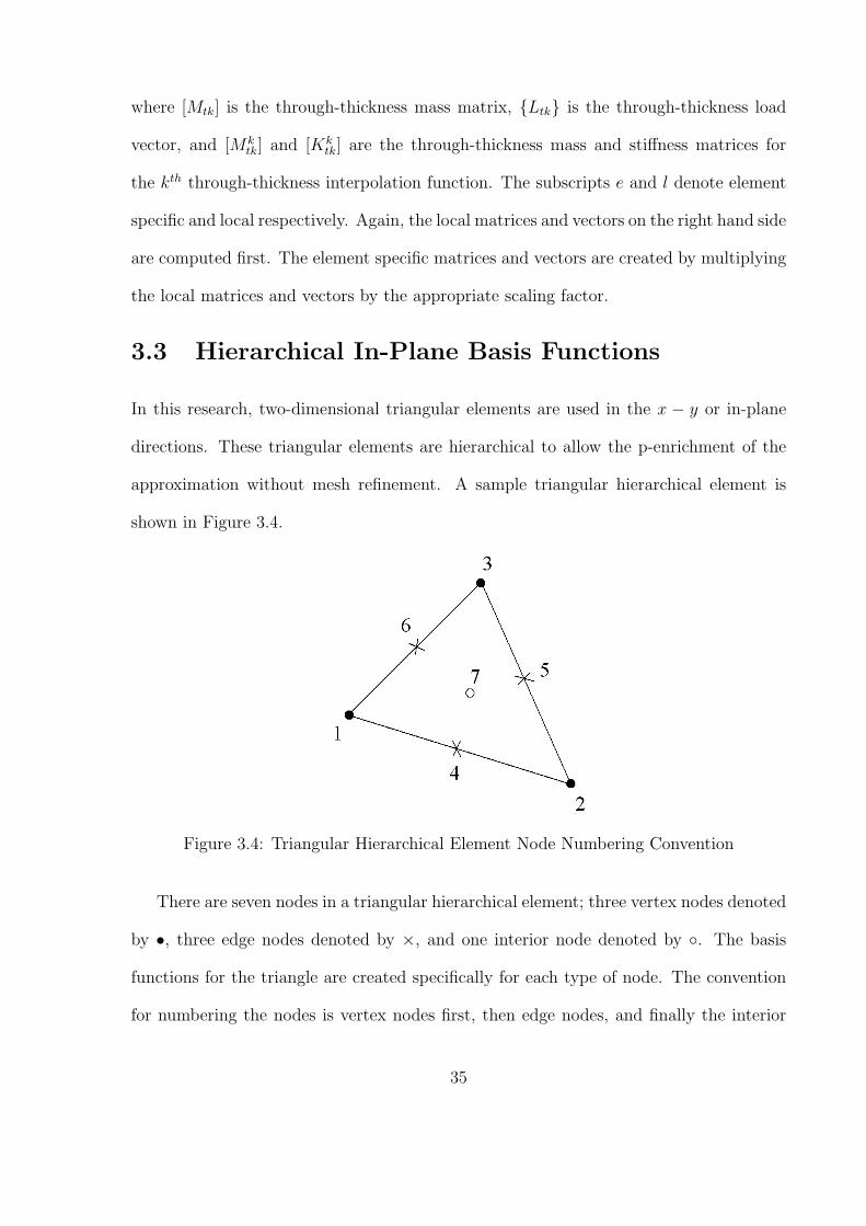
shown in Figure 3.4.

Figure 3.4: Triangular Hierarchical Element Node Numbering Convention

There are seven nodes in a triangular hierarchical element; three vertex nodes denoted

by •, three edge nodes denoted by ×, and one interior node denoted by . The basis

functions for the triangle are created specifically for each type of node. The convention

for numbering the nodes is vertex nodes first, then edge nodes, and finally the interior

35

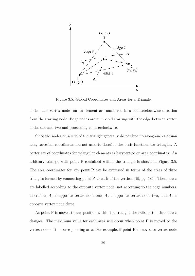
Figure 3.5: Global Coordinates and Areas for a Triangle

node. The vertex nodes on an element are numbered in a counterclockwise direction

from the starting node. Edge nodes are numbered starting with the edge between vertex

nodes one and two and proceeding counterclockwise.

Since the nodes on a side of the triangle generally do not line up along one cartesian

axis, cartesian coordinates are not used to describe the basis functions for triangles. A

better set of coordinates for triangular elements is barycentric or area coordinates. An

arbitrary triangle with point P contained within the triangle is shown in Figure 3.5.

The area coordinates for any point P can be expressed in terms of the areas of three

triangles formed by connecting point P to each of the vertices [19, pg. 186]. These areas

are labelled according to the opposite vertex node, not according to the edge numbers.

Therefore, A1 is opposite vertex node one, A2 is opposite vertex node two, and A3 is

opposite vertex node three.

As point P is moved to any position within the triangle, the ratio of the three areas

changes. The maximum value for each area will occur when point P is moved to the

vertex node of the corresponding area. For example, if point P is moved to vertex node

36

1, A2 = A3 = 0 and A1 is equal to the total area of the triangle. Also note that if point

P is moved to anywhere along edge 2, A1 = 0. Similar relationships also hold for the

other two areas.

The area coordinates for a triangular element are given by

L1 =A1

A

L2 =A2

A(3.24)

L3 =A3

A

where A is the total area of the entire triangle given by

A = A1 + A2 + A3 (3.25)

Since each area coordinate is a ratio of the total area, the maximum value for an area

coordinate is one and the minimum value is zero. The area coordinates are unity when

point P is located on their vertex node and zero along the edge opposite that vertex

node. From (3.24) and (3.25)

L1 + L2 + L3 = 1 (3.26)

Since only two area coordinates are needed to locate a point in the x− y plane, the three

area coordinates specified by L1, L2, and L3 are not linearly independent. Normally when

using area coordinates, L1 and L2 are taken to be independent and L3 is the dependent

area coordinate according to the equation of constraint given in (3.26)

L3 = 1− L1 − L2 (3.27)

Each vertex node of the triangle has one basis function associated with it. The vertex

basis functions capture the linear variation in the temperature approximation over the

element. The basis functions for the vertex nodes of the triangle are given by the area

37

coordinates

φv1 = L1

φv2 = L2 (3.28)

φv3 = L3

where the subscript denotes the node number and the superscript denotes that it is

a vertex basis function. These vertex basis functions are included for any polynomial

approximation of temperature in the in-plane direction of degree pip. For any triangular

element, the number of vertex basis functions, N vip, is three.

Now that the vertex basis functions have been established for a triangular element, the

edge basis functions are defined. The edge basis functions are needed when the polynomial

degree of the temperature approximation over an edge is two or higher, peip ≥ 2. For

peip < 2 there are no edge nodes and only the vertex basis functions are used. The

polynomial degree of the in-plane temperature approximation can be different for each

edge. For an in-plane temperature approximation over an edge of degree peip, there are

peip − 1 edge basis functions for that edge node.

The edge basis functions are created by using the higher-degree one-dimensional hi-

erarchical basis functions from (3.14). An edge coordinate is defined so that the one-

dimensional hierarchical basis is evaluated over the appropriate interval of (−1, 1)

ξe = Lk − Le (3.29)

where ξe is the edge coordinate for edge e, Le is the area coordinate for vertex node e,

and Lk is the area coordinate of the next vertex node, k, in a counterclockwise direction

from vertex node e. Table 3.1 [9, pg. 20] gives the values of e and k for any of the edges.

A quadratic polynomial of the edge coordinate is also used in the formulation of the edge

38

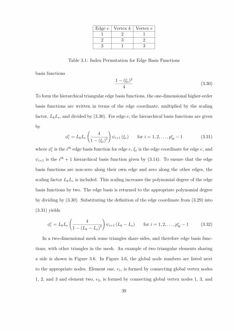
Edge e Vertex k Vertex e1 2 12 3 23 1 3

Table 3.1: Index Permutation for Edge Basis Functions

basis functions

1− (ξe)2

4(3.30)

To form the hierarchical triangular edge basis functions, the one-dimensional higher-order

basis functions are written in terms of the edge coordinate, multiplied by the scaling

factor, LkLe, and divided by (3.30). For edge e, the hierarchical basis functions are given

by

φei = LkLe

(4

1− (ξe)2

)ψi+1 (ξe) for i = 1, 2, . . . , pe

ip − 1 (3.31)

where φei is the ith edge basis function for edge e, ξe is the edge coordinate for edge e, and

ψi+1 is the ith + 1 hierarchical basis function given by (3.14). To ensure that the edge

basis functions are non-zero along their own edge and zero along the other edges, the

scaling factor LkLe is included. This scaling increases the polynomial degree of the edge

basis functions by two. The edge basis is returned to the appropriate polynomial degree

by dividing by (3.30). Substituting the definition of the edge coordinate from (3.29) into

(3.31) yields

φei = LkLe

(4

1− (Lk − Le)2

)ψi+1 (Lk − Le) for i = 1, 2, . . . , pe

ip − 1 (3.32)

In a two-dimensional mesh some triangles share sides, and therefore edge basis func-

tions, with other triangles in the mesh. An example of two triangular elements sharing

a side is shown in Figure 3.6. In Figure 3.6, the global node numbers are listed next

to the appropriate nodes. Element one, e1, is formed by connecting global vertex nodes

1, 2, and 3 and element two, e2, is formed by connecting global vertex nodes 1, 3, and

39

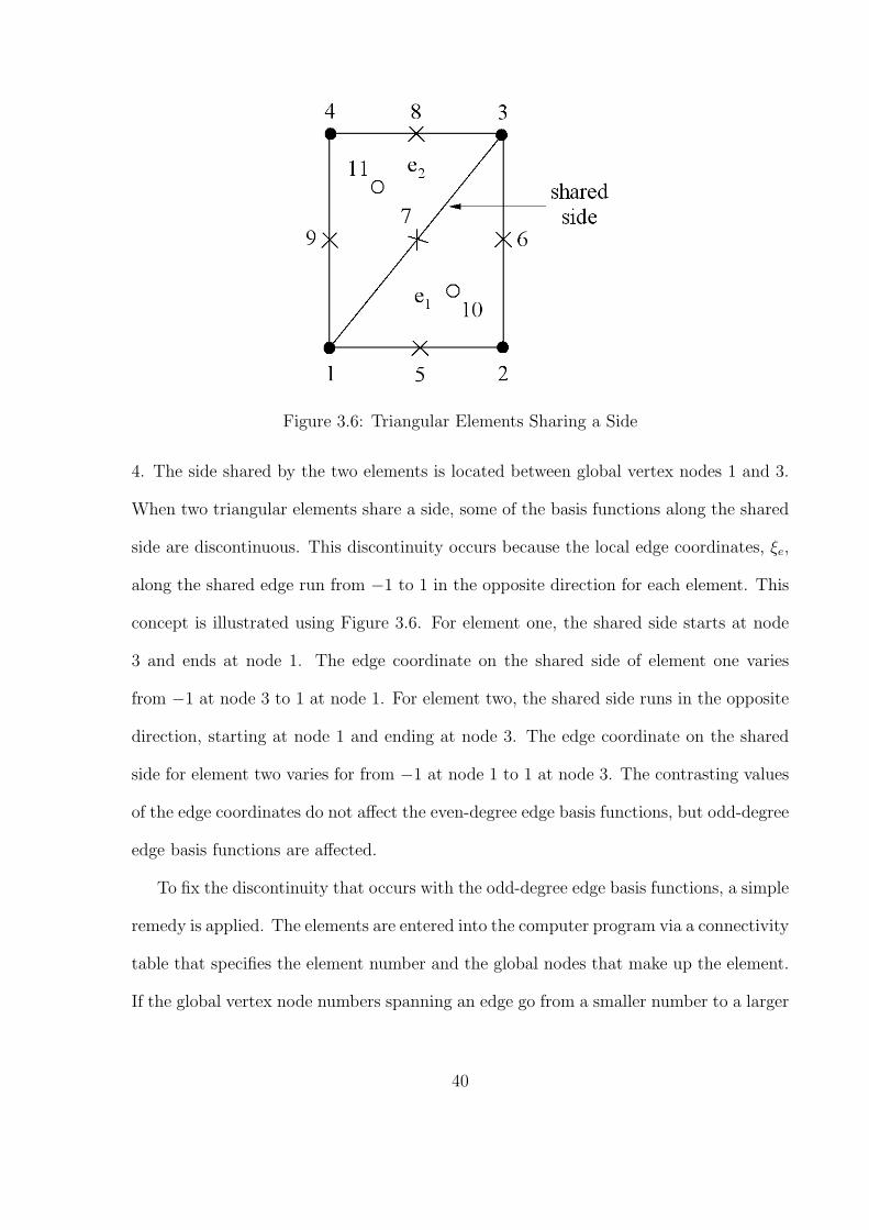
Figure 3.6: Triangular Elements Sharing a Side

4. The side shared by the two elements is located between global vertex nodes 1 and 3.

When two triangular elements share a side, some of the basis functions along the shared

side are discontinuous. This discontinuity occurs because the local edge coordinates, ξe,

along the shared edge run from −1 to 1 in the opposite direction for each element. This

concept is illustrated using Figure 3.6. For element one, the shared side starts at node

3 and ends at node 1. The edge coordinate on the shared side of element one varies

from −1 at node 3 to 1 at node 1. For element two, the shared side runs in the opposite

direction, starting at node 1 and ending at node 3. The edge coordinate on the shared

side for element two varies for from −1 at node 1 to 1 at node 3. The contrasting values

of the edge coordinates do not affect the even-degree edge basis functions, but odd-degree

edge basis functions are affected.

To fix the discontinuity that occurs with the odd-degree edge basis functions, a simple

remedy is applied. The elements are entered into the computer program via a connectivity

table that specifies the element number and the global nodes that make up the element.

If the global vertex node numbers spanning an edge go from a smaller number to a larger

40

number, then every odd-degree edge basis function along that edge is multiplied by −1.

In Figure 3.6 the odd-degree edge basis functions in element one along the sides from

nodes 1 to 2 and 2 to 3 are multiplied by −1. In element two, the odd-degree edge basis

functions along the sides from nodes 1 to 3 and 3 to 4 are multiplied by −1. Multiplying

by −1 reverses the direction of the edge coordinate. By modifying the appropriate edge

basis functions as described above, continuity has been restored to the basis functions

for the elements in Figure 3.6. The elements have also been modified to allow sharing on

any other edge with additional triangular elements.

The basis functions for the internal nodes create higher-degree variation within the

interior of the element. The internal basis functions exist when the polynomial degree of

the temperature approximation over an element is three or higher, pip ≥ 3. For pip < 3

there are no internal nodes. Note that pip may have different values for each element in

the mesh. The vertex and edge basis functions capture the variation over the edges of

the triangle. In order to avoid redundancy, the interior basis functions are designed to

vanish along the edges. A simple function that satisfies these requirements is given by

φi1 = L1L2L3 (3.33)

such that φi1 is the interior basis function for an element with pip = 3. For in-plane

approximations higher than degree three, additional functions are added to the set of the

interior basis. In order to accomplish this, a set of local orthogonal coordinates, α and

β, are defined over the interval (−1, 1)

α = L2 − L1

β = 2L3 − 1 (3.34)

To construct the interior basis functions, consider Pascal’s triangle shown in Table 3.2

where P (α) and P (β) are the Legendre polynomials in terms of the interior coordinates.

41

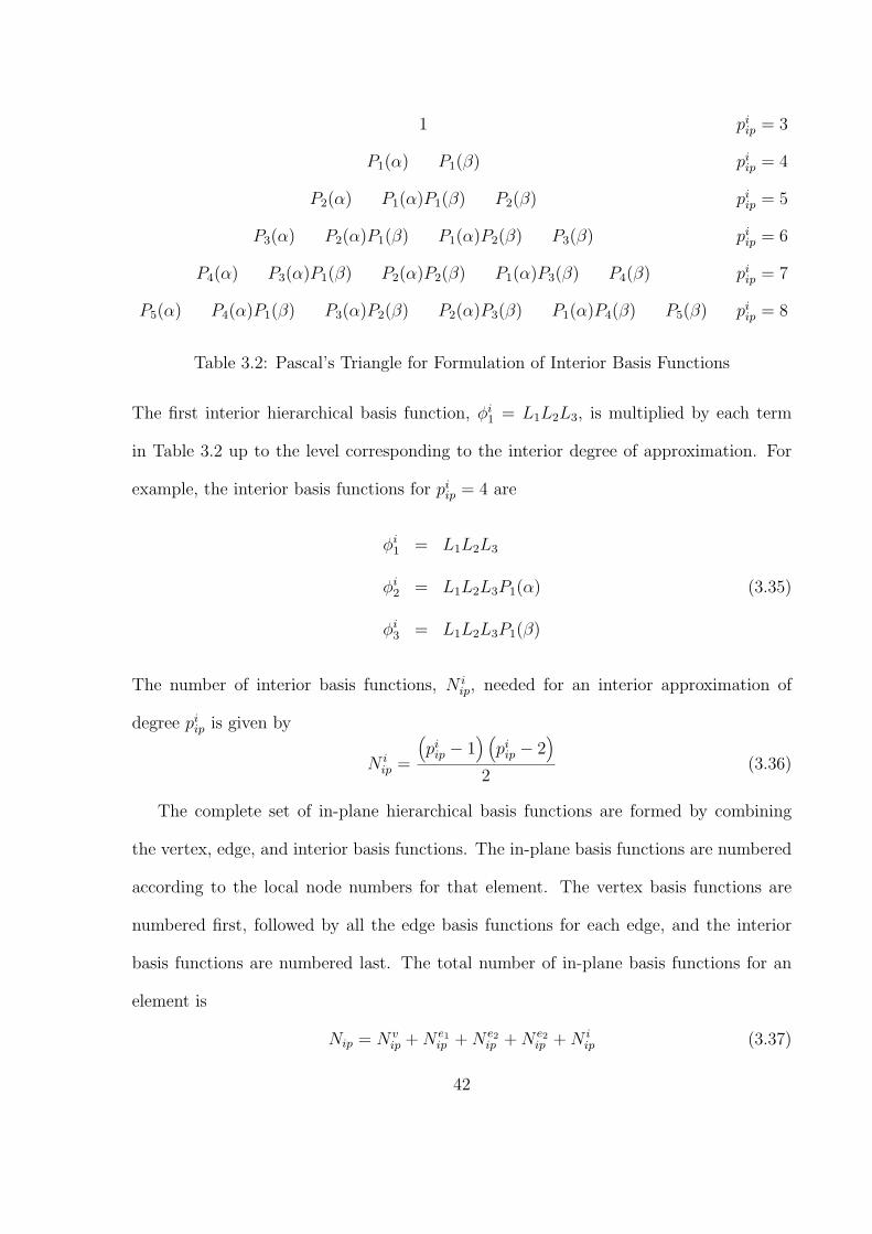
1 piip = 3

P1(α) P1(β) piip = 4

P2(α) P1(α)P1(β) P2(β) piip = 5

P3(α) P2(α)P1(β) P1(α)P2(β) P3(β) piip = 6

P4(α) P3(α)P1(β) P2(α)P2(β) P1(α)P3(β) P4(β) piip = 7

P5(α) P4(α)P1(β) P3(α)P2(β) P2(α)P3(β) P1(α)P4(β) P5(β) piip = 8

Table 3.2: Pascal’s Triangle for Formulation of Interior Basis Functions

The first interior hierarchical basis function, φi1 = L1L2L3, is multiplied by each term

in Table 3.2 up to the level corresponding to the interior degree of approximation. For

example, the interior basis functions for piip = 4 are

φi1 = L1L2L3

φi2 = L1L2L3P1(α) (3.35)

φi3 = L1L2L3P1(β)

The number of interior basis functions, N iip, needed for an interior approximation of

degree piip is given by

N iip =

(pi

ip − 1) (

piip − 2

)

2(3.36)

The complete set of in-plane hierarchical basis functions are formed by combining

the vertex, edge, and interior basis functions. The in-plane basis functions are numbered

according to the local node numbers for that element. The vertex basis functions are

numbered first, followed by all the edge basis functions for each edge, and the interior

basis functions are numbered last. The total number of in-plane basis functions for an

element is

Nip = N vip + N e1

ip + N e2ip + N e2

ip + N iip (3.37)

42

where N vip is the number of vertex basis functions, N e1

ip is the number of edge basis

functions on edge 1, N e2ip is the number of edge basis functions on edge 2, N e3

ip is the

number of edge basis functions on edge 3, and N iip is the number of edge basis functions

within the interior. If the same in-plane approximation degree, pip, is used for all of the

edges and the interior, then the total number of in-plane basis functions for an element

given by (3.37) simplifies to

Nip =(pip + 1) (pip + 2)

2(3.38)

The approximation in the in-plane direction captures the temperature distribution in

the x−y plane. The polynomial degree of approximation for the in-plane direction is the

highest degree term needed in the approximation. The degree of each term is calculated

by adding the degree in x and the degree in y for that term. For example, if the function

2x+3y is to be represented exactly by the in-plane approximation, only the vertex basis

functions are needed since the function is linear in x and linear in y. By contrast, if the

function 2x + 4xy + 3y is to be represented exactly by the in-plane approximation, a

second degree polynomial is needed. This is because the 4xy term is second degree, first

degree in x plus first degree in y. A fifth degree approximation is needed to represent

exactly a function such as 3x2 + 10xy4, first degree in x plus fourth degree in y. A fifth

degree approximation can also exactly represent the function 5x3y2 + 8x5 + 7y5.

The three vertex nodes in Figure 3.5 have global coordinates (x1, y1), (x2, y2), and

(x3, y3). The local area coordinates are used to create local matrices and vectors. These

matrices and vectors are then modified to create element specific matrices and vectors in

the global context. The global coordinates are related to the local coordinates by

x = x1L1 + x2L2 + x3L3

y = y1L1 + y2L2 + y3L3 (3.39)

43

The matrices and vectors that are calculated using the in-plane basis are contained

in (2.37) through (2.40) and (2.44). The local in-plane integrals are calculated first

by integrating over the local element area. These integrals are then mapped from the

local domain to the global domain to create the element specific integrals. In order to

accomplish this, a relation between the element specific differential area, dA, and the

local element area, dAL, is needed. The Jacobian is used to map the differential area

from local to the global coordinates [14, pg. 220-1]

dA = | J | dAL = | J | dL1dL2 (3.40)

where | J | is the absolute value of the Jacobian, J . The Jacobian is given by

J =∂(x, y)

∂(L1, L2)= det

[∂x∂L1

∂y∂L1

∂x∂L2

∂y∂L2

]= det

[x1 − x3 y1 − y3

x2 − x3 y2 − y3

](3.41)

Only L1 and L2 are used since there are only two linearly independent area coordinates.

The Jacobian is constant for any element because the transformation between local and

global coordinates is linear [20]. By using the chain rule of partial differentiation a

relationship between the partial derivatives with respect to local and global coordinates

is established ∂φi

∂L1∂φi

∂L2

=

[∂x∂L1

∂y∂L1

∂x∂L2

∂y∂L2

] ∂φi

∂x∂φi

∂y

(3.42)

The matrix in (3.42) is the same matrix from (3.41). This matrix is known as the Jacobian

matrix, [Jm]. Solving (3.42) for the partial derivatives of the basis functions with respect

to the global variables x and y yields

∂φi

∂x∂φi

∂y

= [Jm]−1

∂φi

∂L1∂φi

∂L2

(3.43)

This relationship is used to convert the in-plane integrals in (2.44) to local integrals and

allow a simple conversion from local to global coordinates.

44

Using (3.40) to modify the in-plane basis in (2.37) through (2.40) and (2.44) and

by pulling the constant Jacobian outside the integrals, a local calculation can be made

instead of an element specific calculation for several matrices

[Mip]e =∫

AφφT dA = | J |

∫

AL

φφT dL1dL2 = | J | [Mip]l (3.44)

Lipe =∫

Aφ dA = | J |

∫

AL

φ dL1dL2 = | J | Lipe (3.45)

[M i

ip

]e=

∫

AφφφT dA = | J |

∫

AL

φφφT dL1dL2 = | J |[M i

ip

]l

(3.46)

where [Mip] is the in-plane mass matrix, Lip is the in-plane load vector, and[M i

ip

]is

the in-plane mass matrix for the ith in-plane interpolation function. Again, the subscripts

e and l denote element specific and local respectively. The local matrices and vectors are

computed first and the element specific matrices and vectors are created by multiplying

the local matrices and vectors by the Jacobian.

The in-plane stiffness matrix for the ith in-plane interpolation function from (2.44) is

[Ki

ip

]e=

∫

Aφi

[∂φ

∂x

∂φ

∂x

T

+∂φ

∂y

∂φ

∂y

T]

dA (3.47)

A transformation from global coordinates to local coordinates for the ith in-plane stiffness

matrix is needed. First, the inverse Jacobian matrix, [Jm]−1 from (3.43) is written in a

convenient form as

[Jm]−1 =

[αx ρx

αy ρy

](3.48)

Using (3.48) to transform from global to local coordinates, the two symmetric matrices

from (3.47) are written as

[∂φ

∂x

∂φ

∂x

T]

=

[(αx

∂φ

∂L1

+ ρx∂φ

∂L2

) (αx

∂φ

∂L1

T

+ ρx∂φ

∂L2

T)]

[∂φ

∂y

∂φ

∂y

T]

=

[(αy

∂φ

∂L1

+ ρy∂φ

∂L2

) (αy

∂φ

∂L1

T

+ ρy∂φ

∂L2

T)]

(3.49)

45

Expanding (3.49)

[∂φ

∂y

∂φ

∂y

T]

=

[(α2

x + α2y

) ∂φ

∂L1

∂φ

∂L1

T

+ (αxρx + αyρy)∂φ

∂L1

∂φ

∂L2

T

+ (αxρx + αyρy)∂φ

∂L2

∂φ

∂L1

T

+(ρ2

x + ρ2y

) ∂φ

∂L2

∂φ

∂L2

T]

(3.50)

Substituting (3.50) and (3.40) into (3.47), the ith in-plane stiffness matrix is written as

[9, pg.53-54]

[Ki

ip

]e

=∫

AL

[(α2

x + α2y

)φi

∂φ

∂L1

∂φ

∂L1

T

+ (αxρx + αyρy) φi∂φ

∂L1

∂φ

∂L2

T

+

(αxρx + αyρy) φi∂φ

∂L2

∂φ

∂L1

T

+(ρ2

x + ρ2y

)φi

∂φ

∂L2

∂φ

∂L2

T]| J | dAL (3.51)

The terms αx, αy, ρx, and ρy are taken from the inverse Jacobian matrix and are constant

over each element. Since these terms and the Jacobian are constant over the element,

they are placed outside the integral and (3.51) becomes

[K i

ip

]e

= | J |[(

α2x + α2

y

) ∫

AL

φi∂φ

∂L1

∂φ

∂L1

T

dAL + (αxρx + αyρy)∫

AL

φi∂φ

∂L1

∂φ

∂L2

T

dAL

+ (αxρx + αyρy)∫

AL

φi∂φ

∂L2

∂φ

∂L1

T

dAL +(ρ2

x + ρ2y

) ∫

AL

φi∂φ

∂L2

∂φ

∂L2

T

dAL

](3.52)

The ith local in-plane stiffness matrices from (3.52) are

[Ki

ip

]1

l=

∫

AL

φi∂φ

∂L1

∂φ

∂L1

T

dAL (3.53)

[Ki

ip

]2

l=

∫

AL

φi∂φ

∂L1

∂φ

∂L2

T

dAL (3.54)

[Ki

ip

]3

l=

∫

AL

φi∂φ

∂L2

∂φ

∂L1

T

dAL (3.55)

[Ki

ip

]4

l=

∫

AL

φi∂φ

∂L2

∂φ

∂L2

T

dAL (3.56)

where the superscripts 1, 2, 3, and 4 denote the four different local in-plane stiffness ma-

trices. The local in-plane stiffness matrices from (3.53) through (3.56) are calculated first.

The ith element specific in-plane stiffness matrix,[K i

ip

]e, is calculated by substituting the

local in-plane stiffness matrices from (3.53) through (3.56) into (3.52).

46

Chapter 4

Interpolation of ThermalConductivity

The thermal conductivity of a material may vary greatly with temperature. This is espe-

cially true when a material is exposed to the broad temperature ranges that are commonly

encountered in aerospace applications. The thermal conductivity of real materials is usu-

ally experimentally determined and tabulated for different temperatures. This chapter

explains the method used to account for the variation of the thermal conductivity as a

function of temperature.

To account for the variation in the thermal conductivity, an iterative process is used.

The approximate temperature distribution from the previous iteration is used to create a

polynomial that mimics the behavior of the thermal conductivity over each element. A set

of sampling points on each element are used to represent the temperature distribution over

the element. Using the values of temperature at these sampling points and the tabulated

values of thermal conductivity, a polynomial is created to represent the variation in the

thermal conductivity over an element.

The polynomial representing the variation of the thermal conductivity over each ele-

ment is created using interpolation. Interpolation is frequently used to fit a polynomial to

data using a set number of points. These points are called sampling points and are used

47

to represent a larger set of data. The interpolant is equal to the values of the thermal

conductivity at the sampling points and provides a smooth polynomial distribution in

between the sampling points. By using an appropriate number of sampling points, the

interpolant approximates the variation in the thermal conductivity over an element.

The interpolant is formed from a set of interpolation functions that are multiplied by

scaling factors and then summed. The thermal conductivity over an element is defined

by (2.33)

ke = χTbn,e =(φ⊗ θ ⊗ ψ

)Tbn,e (4.1)

where φ, θ, ψ are vectors that represent the interpolation functions over the in-plane,

time, and through-thickness dimensions respectively and bn,e is a vector of interpolation

constants that is calculated from an,e.

4.1 Lagrange Interpolation Functions

The Lagrange polynomials are used as interpolation functions in this research. An im-

portant property of the Lagrange interpolation functions is that they are unity at their

node and zero at all other nodes. The interpolation functions over time and in the

through-thickness direction are each a set of one-dimensional Lagrange polynomials. The

interpolation functions for the in-plane dimension are a two-dimensional set of Lagrange

polynomials. The in-plane and through-thickness interpolation functions are the same

functions used by Walker [9].

4.1.1 Time Interpolation Functions

One-dimensional Lagrange interpolation functions are used to approximate the variation

in the thermal conductivity over time. The degree of polynomial approximation for

the thermal conductivity over the time dimension is denoted by rt. To create the time

48

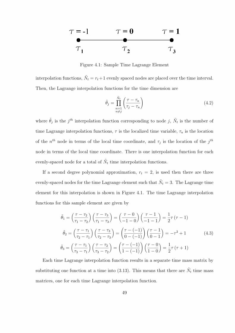
Figure 4.1: Sample Time Lagrange Element

interpolation functions, Nt = rt+1 evenly spaced nodes are placed over the time interval.

Then, the Lagrange interpolation functions for the time dimension are

θj =Nt∏

n=1n 6=j

(τ − τn

τj − τn

)(4.2)

where θj is the jth interpolation function corresponding to node j, Nt is the number of

time Lagrange interpolation functions, τ is the localized time variable, τn is the location

of the nth node in terms of the local time coordinate, and τj is the location of the jth

node in terms of the local time coordinate. There is one interpolation function for each

evenly-spaced node for a total of Nt time interpolation functions.

If a second degree polynomial approximation, rt = 2, is used then there are three

evenly-spaced nodes for the time Lagrange element such that Nt = 3. The Lagrange time

element for this interpolation is shown in Figure 4.1. The time Lagrange interpolation

functions for this sample element are given by

θ1 =(

τ − τ2

τ1 − τ2

) (τ − τ3

τ1 − τ3

)=

(τ − 0

−1− 0

) (τ − 1

−1− 1

)=

1

2τ (τ − 1)

θ2 =(

τ − τ1

τ2 − τ1

) (τ − τ3

τ2 − τ3

)=

(τ − (−1)

0− (−1)

) (τ − 1

0− 1

)= −τ 2 + 1 (4.3)

θ3 =(

τ − τ1

τ3 − τ1

) (τ − τ2

τ3 − τ2

)=

(τ − (−1)

1− (−1)

) (τ − 0

1− 0

)=

1

2τ (τ + 1)

Each time Lagrange interpolation function results in a separate time mass matrix by

substituting one function at a time into (3.13). This means that there are Nt time mass

matrices, one for each time Lagrange interpolation function.

49

4.1.2 Through-Thickness Interpolation Functions

The same interpolation functions used for the time dimension are used for the through-

thickness dimension. The Lagrange interpolation functions for the through-thickness

dimension are

ψk =Ntk∏

n=1n6=k

(η − ηn

ηk − ηn

)(4.4)

where ψk is the kth interpolation function corresponding to node k, Ntk is the number of

through-thickness Lagrange interpolation functions, η is the localized through-thickness

variable, ηn is the location of the nth node in terms of the local through-thickness co-

ordinate, and ηk is the location of the kth node in terms of the local through-thickness

coordinate. There is one interpolation function at each evenly-spaced node for a total

of Ntk through-thickness interpolation functions. Even though the same interpolation

functions are used for the time and through-thickness interpolation, the degree of the

polynomial interpolant may be different and the functions are completely independent

from one another in the finite element formulation.

The through-thickness Lagrange interpolation functions each result in a separate mass

and stiffness matrix by substituting one function at a time into (3.22) and (3.23). There

are Ntk through-thickness mass matrices and Ntk through-thickness stiffness matrices,

one for each through-thickness Lagrange interpolation function.

4.1.3 In-Plane Interpolation Functions

Two-dimensional Lagrange interpolation functions for a triangular element are used to

approximate the variation in the thermal conductivity over the in-plane direction of an

element. The in-plane degree of polynomial approximation for the thermal conductivity

is denoted by rip. The number of terms needed to completely represent a polynomial

of degree rip can be determined from Pascal’s triangle shown in Table 4.1. To create

50

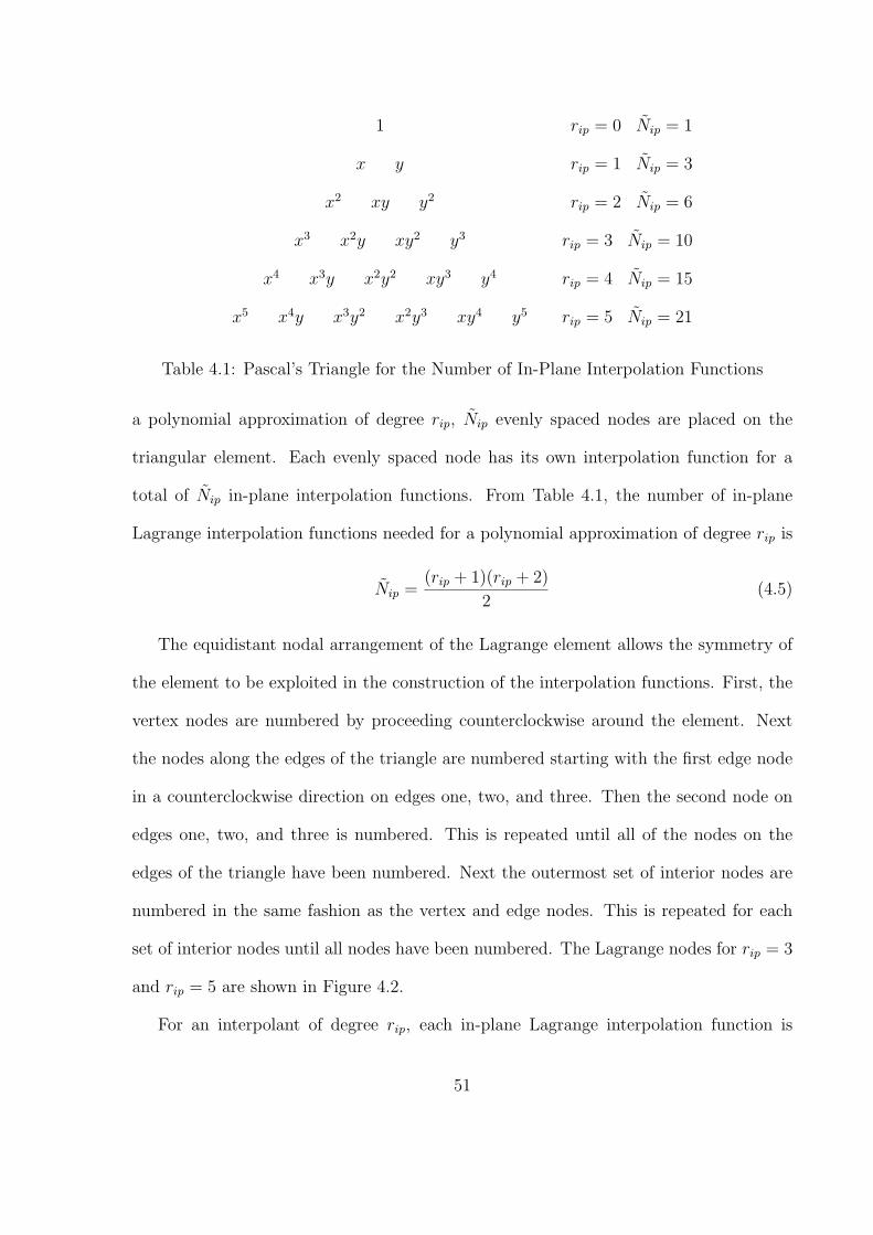
1 rip = 0 Nip = 1

x y rip = 1 Nip = 3

x2 xy y2 rip = 2 Nip = 6

x3 x2y xy2 y3 rip = 3 Nip = 10

x4 x3y x2y2 xy3 y4 rip = 4 Nip = 15

x5 x4y x3y2 x2y3 xy4 y5 rip = 5 Nip = 21

Table 4.1: Pascal’s Triangle for the Number of In-Plane Interpolation Functions

a polynomial approximation of degree rip, Nip evenly spaced nodes are placed on the

triangular element. Each evenly spaced node has its own interpolation function for a

total of Nip in-plane interpolation functions. From Table 4.1, the number of in-plane

Lagrange interpolation functions needed for a polynomial approximation of degree rip is

Nip =(rip + 1)(rip + 2)

2(4.5)

The equidistant nodal arrangement of the Lagrange element allows the symmetry of

the element to be exploited in the construction of the interpolation functions. First, the

vertex nodes are numbered by proceeding counterclockwise around the element. Next

the nodes along the edges of the triangle are numbered starting with the first edge node

in a counterclockwise direction on edges one, two, and three. Then the second node on

edges one, two, and three is numbered. This is repeated until all of the nodes on the

edges of the triangle have been numbered. Next the outermost set of interior nodes are

numbered in the same fashion as the vertex and edge nodes. This is repeated for each

set of interior nodes until all nodes have been numbered. The Lagrange nodes for rip = 3

and rip = 5 are shown in Figure 4.2.

For an interpolant of degree rip, each in-plane Lagrange interpolation function is

51

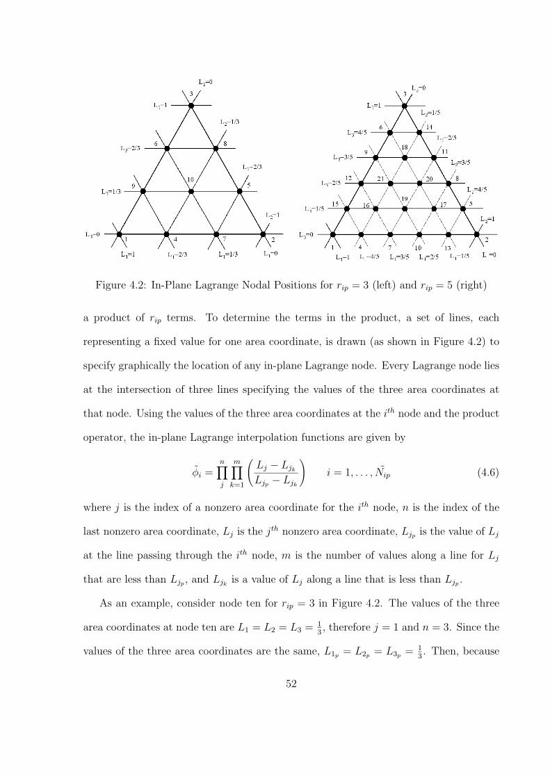
Figure 4.2: In-Plane Lagrange Nodal Positions for rip = 3 (left) and rip = 5 (right)

a product of rip terms. To determine the terms in the product, a set of lines, each

representing a fixed value for one area coordinate, is drawn (as shown in Figure 4.2) to

specify graphically the location of any in-plane Lagrange node. Every Lagrange node lies

at the intersection of three lines specifying the values of the three area coordinates at

that node. Using the values of the three area coordinates at the ith node and the product

operator, the in-plane Lagrange interpolation functions are given by

φi =n∏

j

m∏

k=1

(Lj − Ljk

Ljp − Ljk

)i = 1, . . . , Nip (4.6)

where j is the index of a nonzero area coordinate for the ith node, n is the index of the

last nonzero area coordinate, Lj is the jth nonzero area coordinate, Ljp is the value of Lj

at the line passing through the ith node, m is the number of values along a line for Lj

that are less than Ljp , and Ljkis a value of Lj along a line that is less than Ljp .

As an example, consider node ten for rip = 3 in Figure 4.2. The values of the three

area coordinates at node ten are L1 = L2 = L3 = 13, therefore j = 1 and n = 3. Since the

values of the three area coordinates are the same, L1p = L2p = L3p = 13. Then, because

52

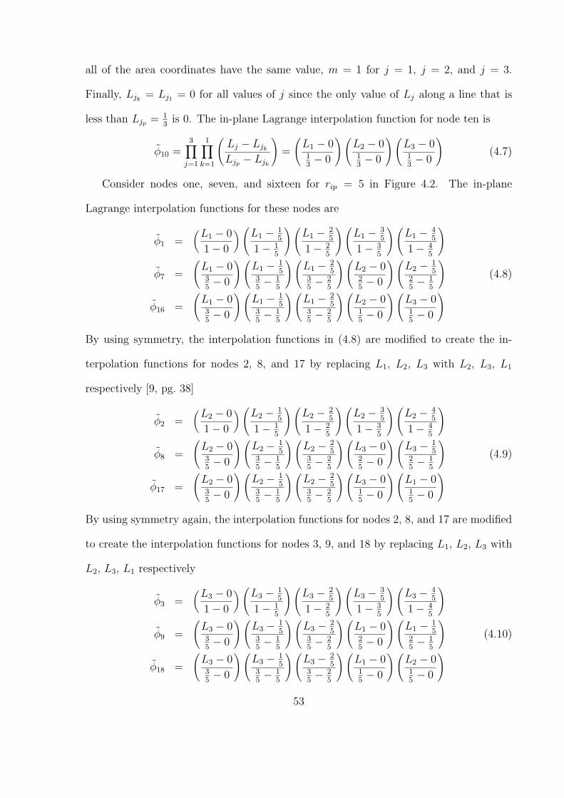
all of the area coordinates have the same value, m = 1 for j = 1, j = 2, and j = 3.

Finally, Ljk= Lj1 = 0 for all values of j since the only value of Lj along a line that is

less than Ljp = 13

is 0. The in-plane Lagrange interpolation function for node ten is

φ10 =3∏

j=1

1∏

k=1

(Lj − Ljk

Ljp − Ljk

)=

(L1 − 013− 0

) (L2 − 013− 0

) (L3 − 013− 0

)(4.7)

Consider nodes one, seven, and sixteen for rip = 5 in Figure 4.2. The in-plane

Lagrange interpolation functions for these nodes are

φ1 =(

L1 − 0

1− 0

) (L1 − 1

5

1− 15

) (L1 − 2

5

1− 25

) (L1 − 3

5

1− 35

) (L1 − 4

5

1− 45

)

φ7 =

(L1 − 035− 0

) (L1 − 1

535− 1

5

) (L1 − 2

535− 2

5

) (L2 − 025− 0

) (L2 − 1

525− 1

5

)(4.8)

φ16 =

(L1 − 035− 0

) (L1 − 1

535− 1

5

) (L1 − 2

535− 2

5

) (L2 − 015− 0

) (L3 − 015− 0

)

By using symmetry, the interpolation functions in (4.8) are modified to create the in-

terpolation functions for nodes 2, 8, and 17 by replacing L1, L2, L3 with L2, L3, L1

respectively [9, pg. 38]

φ2 =(

L2 − 0

1− 0

) (L2 − 1

5

1− 15

) (L2 − 2

5

1− 25

) (L2 − 3

5

1− 35

) (L2 − 4

5

1− 45

)

φ8 =

(L2 − 035− 0

) (L2 − 1

535− 1

5

) (L2 − 2

535− 2

5

) (L3 − 025− 0

) (L3 − 1

525− 1

5

)(4.9)

φ17 =

(L2 − 035− 0

) (L2 − 1

535− 1

5

) (L2 − 2

535− 2

5

) (L3 − 015− 0

) (L1 − 015− 0

)

By using symmetry again, the interpolation functions for nodes 2, 8, and 17 are modified

to create the interpolation functions for nodes 3, 9, and 18 by replacing L1, L2, L3 with

L2, L3, L1 respectively

φ3 =(

L3 − 0

1− 0

) (L3 − 1

5

1− 15

) (L3 − 2

5

1− 25

) (L3 − 3

5

1− 35

) (L3 − 4

5

1− 45

)

φ9 =

(L3 − 035− 0

) (L3 − 1

535− 1

5

) (L3 − 2

535− 2

5

) (L1 − 025− 0

) (L1 − 1

525− 1

5

)(4.10)

φ18 =

(L3 − 035− 0

) (L3 − 1

535− 1

5

) (L3 − 2

535− 2

5

) (L1 − 015− 0

) (L2 − 015− 0

)

53

Each in-plane Lagrange interpolation function results in a separate mass and stiffness

matrix by substituting one function at a time into (3.46) and (3.52). Therefore there are

Nip in-plane mass matrices and Nip in-plane stiffness matrices for each element, one for

each in-plane Lagrange interpolation function.

4.2 Optimization of Sampling Points

A sampling point is defined by a set of local coordinates specifying the location of the

in-plane, time, and through-thickness coordinates in an element. The choice of sampling

points has a substantial effect on the quality of the interpolant that approximates the

variation in the thermal conductivity over an element. Using evenly spaced sampling

points often results in Runge’s Phenomenon, where the resulting interpolant oscillates

wildly near the ends of the interval [21, pg. 295]. To minimize this oscillation, the

Chebyshev points are biased toward the ends of the one-dimensional element [9, pg. 42]

and the Fekete points are biased towards the vertices of the triangle [23]. To reduce

Runge’s Phenomenon, the Chebyshev and Fekete sampling points used by Walker [9] are

also used in this research.

The zeros of the Chebyshev polynomial are the optimal set of sampling points for a

one-dimensional element in the sense that they minimize the error of the interpolant in

the least squares sense. The coordinate of the kth Chebyshev point for an interpolant of

degree rtk is determined from

ηk = cos

(k − 1

2

)π

rtk − 1

k = 1, 2, . . . , rtk + 1 (4.11)

such that each ηk is a zero of the Chebyshev polynomial of degree rtk + 1 [22]. The

Chebyshev points are used for the time interpolation in addition to the through-thickness

interpolation.

54

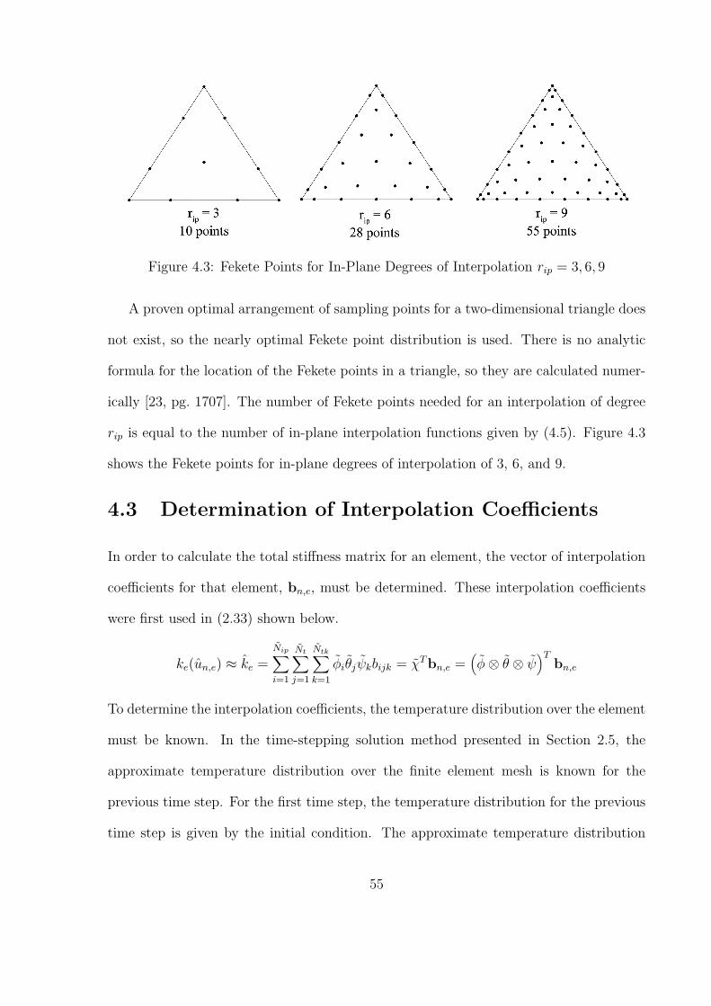
Figure 4.3: Fekete Points for In-Plane Degrees of Interpolation rip = 3, 6, 9

A proven optimal arrangement of sampling points for a two-dimensional triangle does

not exist, so the nearly optimal Fekete point distribution is used. There is no analytic

formula for the location of the Fekete points in a triangle, so they are calculated numer-

ically [23, pg. 1707]. The number of Fekete points needed for an interpolation of degree

rip is equal to the number of in-plane interpolation functions given by (4.5). Figure 4.3

shows the Fekete points for in-plane degrees of interpolation of 3, 6, and 9.

4.3 Determination of Interpolation Coefficients

In order to calculate the total stiffness matrix for an element, the vector of interpolation

coefficients for that element, bn,e, must be determined. These interpolation coefficients

were first used in (2.33) shown below.

ke(un,e) ≈ ke =Nip∑

i=1

Nt∑

j=1

Ntk∑

k=1

φiθjψkbijk = χTbn,e =(φ⊗ θ ⊗ ψ

)Tbn,e

To determine the interpolation coefficients, the temperature distribution over the element

must be known. In the time-stepping solution method presented in Section 2.5, the

approximate temperature distribution over the finite element mesh is known for the

previous time step. For the first time step, the temperature distribution for the previous

time step is given by the initial condition. The approximate temperature distribution

55

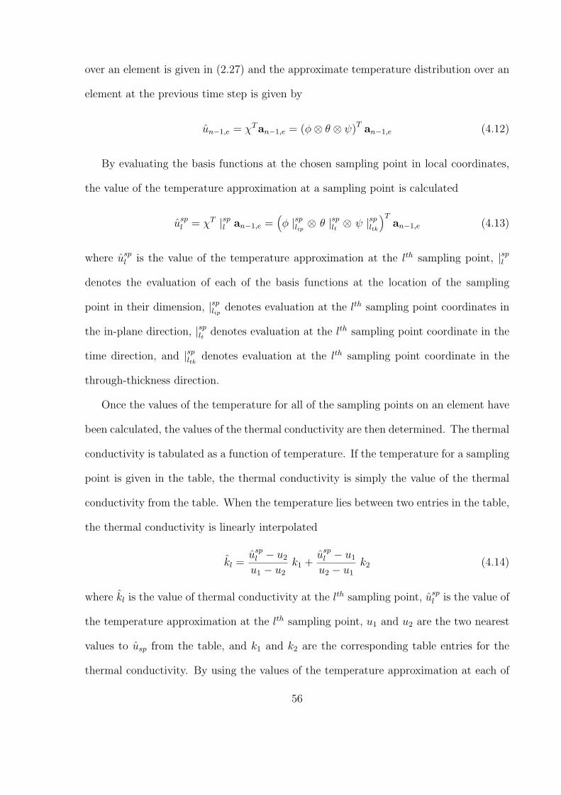
over an element is given in (2.27) and the approximate temperature distribution over an

element at the previous time step is given by

un−1,e = χTan−1,e = (φ⊗ θ ⊗ ψ)T an−1,e (4.12)

By evaluating the basis functions at the chosen sampling point in local coordinates,

the value of the temperature approximation at a sampling point is calculated

uspl = χT |spl an−1,e =

(φ |splip ⊗ θ |splt ⊗ ψ |spltk

)Tan−1,e (4.13)

where uspl is the value of the temperature approximation at the lth sampling point, |spl

denotes the evaluation of each of the basis functions at the location of the sampling

point in their dimension, |splip denotes evaluation at the lth sampling point coordinates in

the in-plane direction, |splt denotes evaluation at the lth sampling point coordinate in the

time direction, and |spltk denotes evaluation at the lth sampling point coordinate in the

through-thickness direction.

Once the values of the temperature for all of the sampling points on an element have

been calculated, the values of the thermal conductivity are then determined. The thermal

conductivity is tabulated as a function of temperature. If the temperature for a sampling

point is given in the table, the thermal conductivity is simply the value of the thermal

conductivity from the table. When the temperature lies between two entries in the table,

the thermal conductivity is linearly interpolated

kl =usp

l − u2

u1 − u2

k1 +usp

l − u1

u2 − u1

k2 (4.14)

where kl is the value of thermal conductivity at the lth sampling point, uspl is the value of

the temperature approximation at the lth sampling point, u1 and u2 are the two nearest

values to usp from the table, and k1 and k2 are the corresponding table entries for the

thermal conductivity. By using the values of the temperature approximation at each of

56

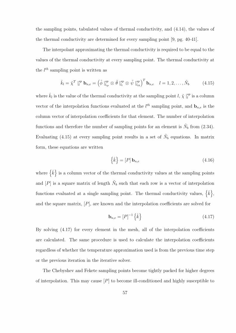
the sampling points, tabulated values of thermal conductivity, and (4.14), the values of

the thermal conductivity are determined for every sampling point [9, pg. 40-41].

The interpolant approximating the thermal conductivity is required to be equal to the

values of the thermal conductivity at every sampling point. The thermal conductivity at

the lth sampling point is written as

kl = χT |spl bn,e =(φ |splip ⊗ θ |splt ⊗ ψ |spltk

)Tbn,e l = 1, 2, . . . , Nb (4.15)

where kl is the value of the thermal conductivity at the sampling point l, χ |spl is a column

vector of the interpolation functions evaluated at the lth sampling point, and bn,e is the

column vector of interpolation coefficients for that element. The number of interpolation

functions and therefore the number of sampling points for an element is Nb from (2.34).

Evaluating (4.15) at every sampling point results in a set of Nb equations. In matrix

form, these equations are written

k

= [P ]bn,e (4.16)

wherek

is a column vector of the thermal conductivity values at the sampling points

and [P ] is a square matrix of length Nb such that each row is a vector of interpolation

functions evaluated at a single sampling point. The thermal conductivity values,k,

and the square matrix, [P ], are known and the interpolation coefficients are solved for

bn,e = [P ]−1k

(4.17)

By solving (4.17) for every element in the mesh, all of the interpolation coefficients

are calculated. The same procedure is used to calculate the interpolation coefficients

regardless of whether the temperature approximation used is from the previous time step

or the previous iteration in the iterative solver.

The Chebyshev and Fekete sampling points become tightly packed for higher degrees

of interpolation. This may cause [P ] to become ill-conditioned and highly susceptible to

57

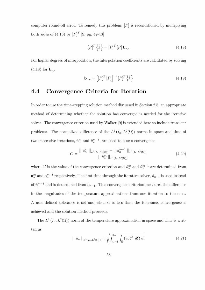
computer round-off error. To remedy this problem, [P ] is reconditioned by multiplying

both sides of (4.16) by [P ]T [9, pg. 42-43]

[P ]Tk

= [P ]T [P ]bn,e (4.18)

For higher degrees of interpolation, the interpolation coefficients are calculated by solving

(4.18) for bn,e

bn,e =[[P ]T [P ]

]−1[P ]T

k

(4.19)

4.4 Convergence Criteria for Iteration

In order to use the time-stepping solution method discussed in Section 2.5, an appropriate

method of determining whether the solution has converged is needed for the iterative

solver. The convergence criterion used by Walker [9] is extended here to include transient

problems. The normalized difference of the L2 (In, L2(Ω)) norms in space and time of

two successive iterations, umn and um−1

n , are used to assess convergence

C =|| um

n ||L2(In,L2(Ω)) − || um−1n ||L2(In,L2(Ω))

|| umn ||L2(In,L2(Ω))

(4.20)

where C is the value of the convergence criterion and umn and um−1

n are determined from

amn and am−1

n respectively. The first time through the iterative solver, un−1 is used instead

of um−1n and is determined from an−1. This convergence criterion measures the difference

in the magnitudes of the temperature approximations from one iteration to the next.

A user defined tolerance is set and when C is less than the tolerance, convergence is

achieved and the solution method proceeds.

The L2 (In, L2(Ω)) norm of the temperature approximation in space and time is writ-

ten as

|| un ||L2(In,L2(Ω)) =

√∫ tn

tn−1

∫

Ω(un)2 dΩ dt (4.21)

58

Substituting for un defined in (2.17) and considering all of the elements at a time step

|| un ||L2(In,L2(Ω)) =Ne∑

e=1

√aT

n,e

[∫ tn

tn−1

∫

Ωe

χχT dΩ dt]an,e (4.22)

then by applying (2.27) and reorganizing,

|| un ||L2(In,L2(Ω)) =Ne∑

e=1

√√√√aTn,e

[∫

Ae

φφT dAe ⊗∫ tn

tn−1θθT dt

∫ d2

− d2

ψψT dz

]an,e (4.23)

Note that the in-plane and through-thickness matrices shown here have already been

calculated to form [Ce]. The time mass matrix can be calculated by using a property of

the Lagrange interpolation functions. The sum of the Lagrange interpolation functions

at any point on the domain is one. This allows the time mass matrix to be calculated by

summing over all of the time mass matrices from (3.13)

[Mt]e =∫ tn

tn−1θθT dt =

∆t

2

Nt∑

j=1

∫ 1

−1θjθθ

T dτ =∆t

2

Nt∑

j=1

[M jt ]l (4.24)

This concept also applies to the in-plane and through-thickness matrices. Any element

matrix can be created by summing over all of the corresponding matrices containing

Lagrange interpolation functions.

Finally, by using the element matrices from (3.20), (3.44), and (4.24), the two different

terms in (4.20) are calculated using matrices that have already been determined

|| umn ||L2(In,L2(Ω)) =

Ne∑

e=1

√(am

n,e

)T [[Mip]e ⊗ [Mt]e ⊗ [Mtk]e

]am

n,e (4.25)

|| um−1n ||L2(In,L2(Ω)) =

Ne∑

e=1

√(am−1

n,e

)T [[Mip]e ⊗ [Mt]e ⊗ [Mtk]e

]am−1

n,e (4.26)

59

Chapter 5

Computer Implementation

The finite element formulation presented in Chapter 2 is implemented in a FORTRAN

program to validate the method. The program is entitled p-Version Nonlinear Discon-

tinuous Galerkin Structurally Compatible Heat Transfer (ndgSCHTp). The original pro-

gram was created by Dr. Kim S. Bey at NASA’s Langley Research Center and was

entitled Structurally Compatible Heat Transfer (SCHT) [24]. SCHT used traditional

linear triangular elements in the in-plane direction combined with hierarchical elements

in the through thickness direction. SCHT was capable of performing transient or steady-

state conduction heat transfer in two or three-dimensions. Tomey modified SCHT to

include hierarchical p-version functions in the in-plane direction. This version was enti-

tled dgSCHTp and could be used for layered materials with constant anisotropic prop-

erties [7]. Walker modified dgSCHTp to analyze nonlinear steady-state problems with

thermal conductivity varying as a function of temperature. Walker’s version was entitled

nSCHTp, for p-version Nonlinear Structurally Compatible Heat Transfer, and did not

allow layered or anisotropic materials [9].

The current version (ndgSCTHp) uses p-version elements in space and time and

accounts for variations in the thermal conductivity as a function of temperature. The

discontinuous Galerkin method is used in time. The operational order for ndgSCHTp

with the modifications made for this research is shown in Figure 5.1. Currently the code

60

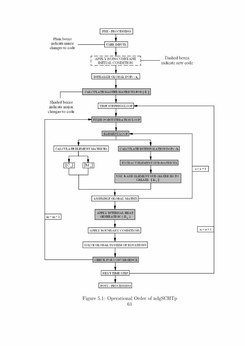
Figure 5.1: Operational Order of ndgSCHTp61

only allows single isotropic materials, but the formulation could be extended to layered

anisotropic materials.

5.1 Integration

Numerous integrals must be evaluated to calculate the matrices and vectors from the finite

element formulation. Several techniques are used to evaluate the integrals as efficiently

and accurately as possible.

The capacitance matrix, [Ce], and mass matrices, [M++e ] and [M−+

e ], in (2.37) through

(2.39) contain integrals involving the in-plane, time, and through-thickness basis func-

tions. The in-plane mass matrix is integrated using the symmetrical Gaussian quadrature

method that utilizes area coordinates and is more efficient than the Gaussian prod-

uct method [25]. The time convective matrix, [Vt]l in (3.9), is integrated using one-

dimensional Gauss-Legendre numerical quadrature [13, pg. 254-8]. The through-thickness

mass matrix, [Mtk]l in (3.20), is integrated analytically since the integrand is a simple

polynomial. The exact integrals for the through-thickness mass matrices were hard coded

into ndgSCHTp.

The stiffness matrix, [Ke (an,e)], in (2.44) contains in-plane, time, and through-

thickness integrations involving interpolation and basis functions. Numerical quadrature

is used to calculate all of the necessary integrals for the stiffness matrix. For the in-

plane integrals in the stiffness matrix, the Fekete sampling points are used as integration

points [23]. The numerical integration using Fekete points is computationally expensive

because it uses more integration points than gaussian quadrature. The time mass ma-

trices, through-thickness mass, and through-thickness stiffness matrices are integrated

using one-dimensional Gauss-Legendre numerical quadrature.

The load vector, He, from (2.40) is made up of the source term component contain-

62

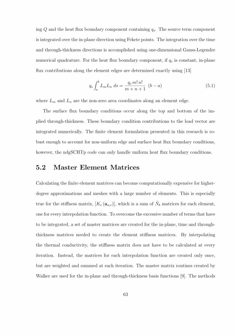
ing Q and the heat flux boundary component containing qs. The source term component

is integrated over the in-plane direction using Fekete points. The integration over the time

and through-thickness directions is accomplished using one-dimensional Gauss-Legendre

numerical quadrature. For the heat flux boundary component, if qs is constant, in-plane

flux contributions along the element edges are determined exactly using [13]

qs

∫ b

aLmLn ds =

qs m! n!

m + n + 1(b− a) (5.1)

where Lm and Ln are the non-zero area coordinates along an element edge.

The surface flux boundary conditions occur along the top and bottom of the im-

plied through-thickness. These boundary condition contributions to the load vector are

integrated numerically. The finite element formulation presented in this research is ro-

bust enough to account for non-uniform edge and surface heat flux boundary conditions,

however, the ndgSCHTp code can only handle uniform heat flux boundary conditions.

5.2 Master Element Matrices

Calculating the finite element matrices can become computationally expensive for higher-

degree approximations and meshes with a large number of elements. This is especially

true for the stiffness matrix, [Ke (an,e)], which is a sum of Nb matrices for each element,

one for every interpolation function. To overcome the excessive number of terms that have

to be integrated, a set of master matrices are created for the in-plane, time and through-

thickness matrices needed to create the element stiffness matrices. By interpolating

the thermal conductivity, the stiffness matrix does not have to be calculated at every

iteration. Instead, the matrices for each interpolation function are created only once,

but are weighted and summed at each iteration. The master matrix routines created by

Walker are used for the in-plane and through-thickness basis functions [9]. The methods

63

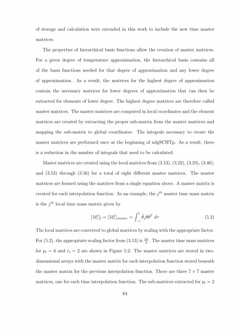
of storage and calculation were extended in this work to include the new time master

matrices.

The properties of hierarchical basis functions allow the creation of master matrices.

For a given degree of temperature approximation, the hierarchical basis contains all

of the basis functions needed for that degree of approximation and any lower degree

of approximation. As a result, the matrices for the highest degree of approximation

contain the necessary matrices for lower degrees of approximation that can then be

extracted for elements of lower degree. The highest degree matrices are therefore called

master matrices. The master matrices are computed in local coordinates and the element

matrices are created by extracting the proper sub-matrix from the master matrices and

mapping the sub-matrix to global coordinates. The integrals necessary to create the

master matrices are performed once at the beginning of ndgSCHTp. As a result, there

is a reduction in the number of integrals that need to be calculated.

Master matrices are created using the local matrices from (3.13), (3.22), (3.23), (3.46),

and (3.53) through (3.56) for a total of eight different master matrices. The master

matrices are formed using the matrices from a single equation above. A master matrix is

created for each interpolation function. As an example, the jth master time mass matrix

is the jth local time mass matrix given by

[M jt ]l = [M j

t ]master =∫ 1

−1θjθθ

T dτ (5.2)

The local matrices are converted to global matrices by scaling with the appropriate factor.

For (5.2), the appropriate scaling factor from (3.13) is ∆t2

. The master time mass matrices

for pt = 6 and rt = 2 are shown in Figure 5.2. The master matrices are stored in two-

dimensional arrays with the master matrix for each interpolation function stored beneath

the master matrix for the previous interpolation function. There are three 7× 7 master

matrices, one for each time interpolation function. The sub-matrices extracted for pt = 2

64

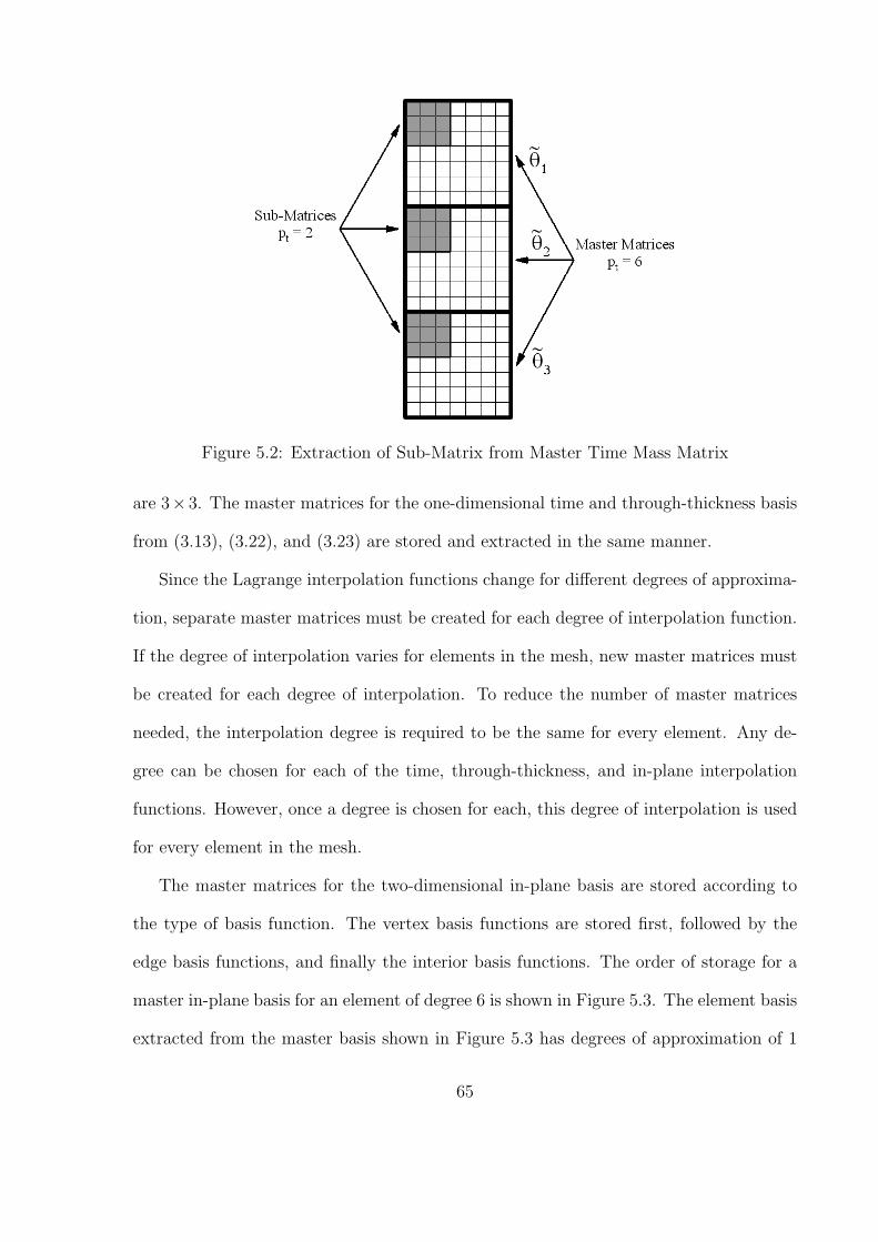
Figure 5.2: Extraction of Sub-Matrix from Master Time Mass Matrix

are 3× 3. The master matrices for the one-dimensional time and through-thickness basis

from (3.13), (3.22), and (3.23) are stored and extracted in the same manner.

Since the Lagrange interpolation functions change for different degrees of approxima-

tion, separate master matrices must be created for each degree of interpolation function.

If the degree of interpolation varies for elements in the mesh, new master matrices must

be created for each degree of interpolation. To reduce the number of master matrices

needed, the interpolation degree is required to be the same for every element. Any de-

gree can be chosen for each of the time, through-thickness, and in-plane interpolation

functions. However, once a degree is chosen for each, this degree of interpolation is used

for every element in the mesh.

The master matrices for the two-dimensional in-plane basis are stored according to

the type of basis function. The vertex basis functions are stored first, followed by the

edge basis functions, and finally the interior basis functions. The order of storage for a

master in-plane basis for an element of degree 6 is shown in Figure 5.3. The element basis

extracted from the master basis shown in Figure 5.3 has degrees of approximation of 1

65

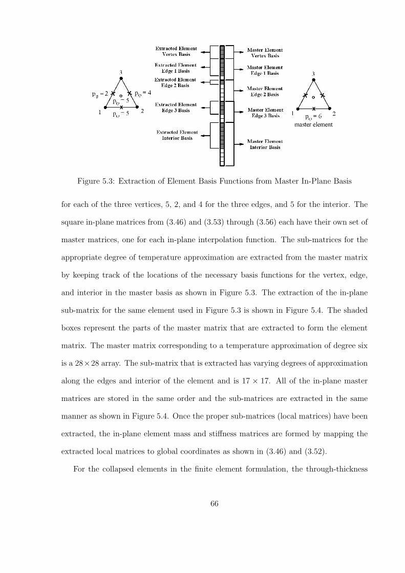
Figure 5.3: Extraction of Element Basis Functions from Master In-Plane Basis

for each of the three vertices, 5, 2, and 4 for the three edges, and 5 for the interior. The

square in-plane matrices from (3.46) and (3.53) through (3.56) each have their own set of

master matrices, one for each in-plane interpolation function. The sub-matrices for the

appropriate degree of temperature approximation are extracted from the master matrix

by keeping track of the locations of the necessary basis functions for the vertex, edge,

and interior in the master basis as shown in Figure 5.3. The extraction of the in-plane

sub-matrix for the same element used in Figure 5.3 is shown in Figure 5.4. The shaded

boxes represent the parts of the master matrix that are extracted to form the element

matrix. The master matrix corresponding to a temperature approximation of degree six

is a 28×28 array. The sub-matrix that is extracted has varying degrees of approximation

along the edges and interior of the element and is 17 × 17. All of the in-plane master

matrices are stored in the same order and the sub-matrices are extracted in the same

manner as shown in Figure 5.4. Once the proper sub-matrices (local matrices) have been

extracted, the in-plane element mass and stiffness matrices are formed by mapping the

extracted local matrices to global coordinates as shown in (3.46) and (3.52).

For the collapsed elements in the finite element formulation, the through-thickness

66

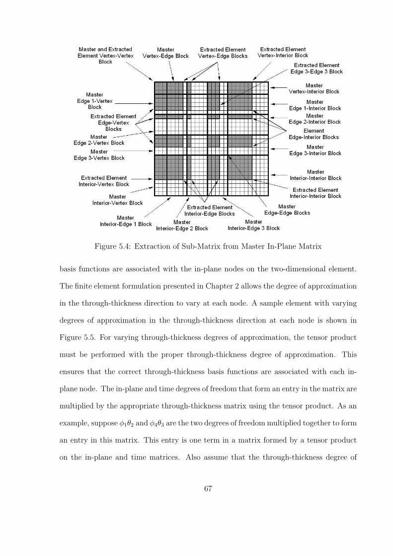
Figure 5.4: Extraction of Sub-Matrix from Master In-Plane Matrix

basis functions are associated with the in-plane nodes on the two-dimensional element.

The finite element formulation presented in Chapter 2 allows the degree of approximation

in the through-thickness direction to vary at each node. A sample element with varying

degrees of approximation in the through-thickness direction at each node is shown in

Figure 5.5. For varying through-thickness degrees of approximation, the tensor product

must be performed with the proper through-thickness degree of approximation. This

ensures that the correct through-thickness basis functions are associated with each in-

plane node. The in-plane and time degrees of freedom that form an entry in the matrix are

multiplied by the appropriate through-thickness matrix using the tensor product. As an

example, suppose φ1θ2 and φ4θ3 are the two degrees of freedom multiplied together to form

an entry in this matrix. This entry is one term in a matrix formed by a tensor product

on the in-plane and time matrices. Also assume that the through-thickness degree of

67

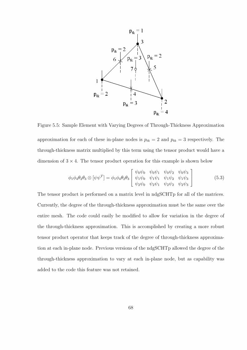
Figure 5.5: Sample Element with Varying Degrees of Through-Thickness Approximation

approximation for each of these in-plane nodes is ptk = 2 and ptk = 3 respectively. The

through-thickness matrix multiplied by this term using the tensor product would have a

dimension of 3× 4. The tensor product operation for this example is shown below

φ1φ4θ2θ3 ⊗ [ψψT ] = φ1φ4θ2θ3

ψ0ψ0 ψ0ψ1 ψ0ψ2 ψ0ψ3

ψ1ψ0 ψ1ψ1 ψ1ψ2 ψ1ψ3

ψ2ψ0 ψ2ψ1 ψ2ψ2 ψ2ψ3

(5.3)

The tensor product is performed on a matrix level in ndgSCHTp for all of the matrices.

Currently, the degree of the through-thickness approximation must be the same over the

entire mesh. The code could easily be modified to allow for variation in the degree of

the through-thickness approximation. This is accomplished by creating a more robust

tensor product operator that keeps track of the degree of through-thickness approxima-

tion at each in-plane node. Previous versions of the ndgSCHTp allowed the degree of the

through-thickness approximation to vary at each in-plane node, but as capability was

added to the code this feature was not retained.

68

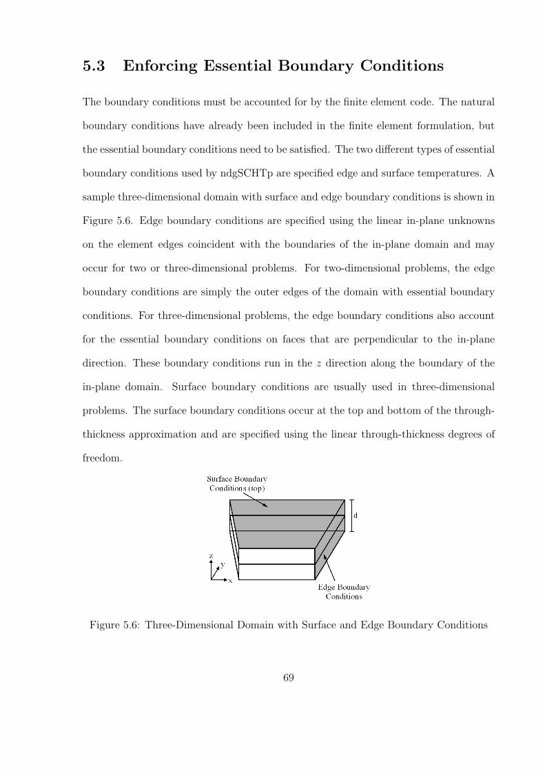
5.3 Enforcing Essential Boundary Conditions

The boundary conditions must be accounted for by the finite element code. The natural

boundary conditions have already been included in the finite element formulation, but

the essential boundary conditions need to be satisfied. The two different types of essential

boundary conditions used by ndgSCHTp are specified edge and surface temperatures. A

sample three-dimensional domain with surface and edge boundary conditions is shown in

Figure 5.6. Edge boundary conditions are specified using the linear in-plane unknowns

on the element edges coincident with the boundaries of the in-plane domain and may

occur for two or three-dimensional problems. For two-dimensional problems, the edge

boundary conditions are simply the outer edges of the domain with essential boundary

conditions. For three-dimensional problems, the edge boundary conditions also account

for the essential boundary conditions on faces that are perpendicular to the in-plane

direction. These boundary conditions run in the z direction along the boundary of the

in-plane domain. Surface boundary conditions are usually used in three-dimensional

problems. The surface boundary conditions occur at the top and bottom of the through-

thickness approximation and are specified using the linear through-thickness degrees of

freedom.

Figure 5.6: Three-Dimensional Domain with Surface and Edge Boundary Conditions

69

To capture the edge boundary conditions, the appropriate in-plane unknowns are

modified. For a constant temperature on the edges, all of the higher-degree in-plane un-

knowns on the boundary are set to zero. The linear in-plane unknowns on the boundary

are set equal to the boundary condition temperature. For the surface boundary condi-

tions, the appropriate through-thickness unknowns are assigned values. For a constant

or linear surface temperature, all of the higher-degree through-thickness unknowns are

set to zero. The linear through-thickness degrees of freedom are set equal to the constant

boundary condition temperature. If the surface temperature has different values on the

top and bottom, then the linear through-thickness unknowns are set to the corresponding

temperature. The through-thickness unknowns corresponding to ψ0 are set to the surface

temperature of the bottom surface. The degrees of freedom corresponding to ψ1 are set

to the surface temperature of the top surface.

If the boundary condition is a polynomial in space, the unknowns corresponding to the

polynomial are used to account for the boundary condition. The unknowns are defined so

that the polynomial distribution on the boundary is reflected in the solution. Unknowns

corresponding to basis functions with degrees higher than that of the polynomial are set

to zero.

To enforce essential boundary conditions, ndgSCHTp uses the penalty method. After

the global matrix and source vector are assembled at each time step, the penalty method is

applied to ensure that the known degrees of freedom attain the proper values. The penalty

parameter is a very large number used to implement the method and in ndgSCHTp, the

penalty parameter is 1035. As an example, suppose that the global matrix is 5 × 5, the

essential boundary condition has a constant value of Tbc, and the essential boundary

condition occurs at unknowns a1 and a4. The penalty method for this example is shown

70

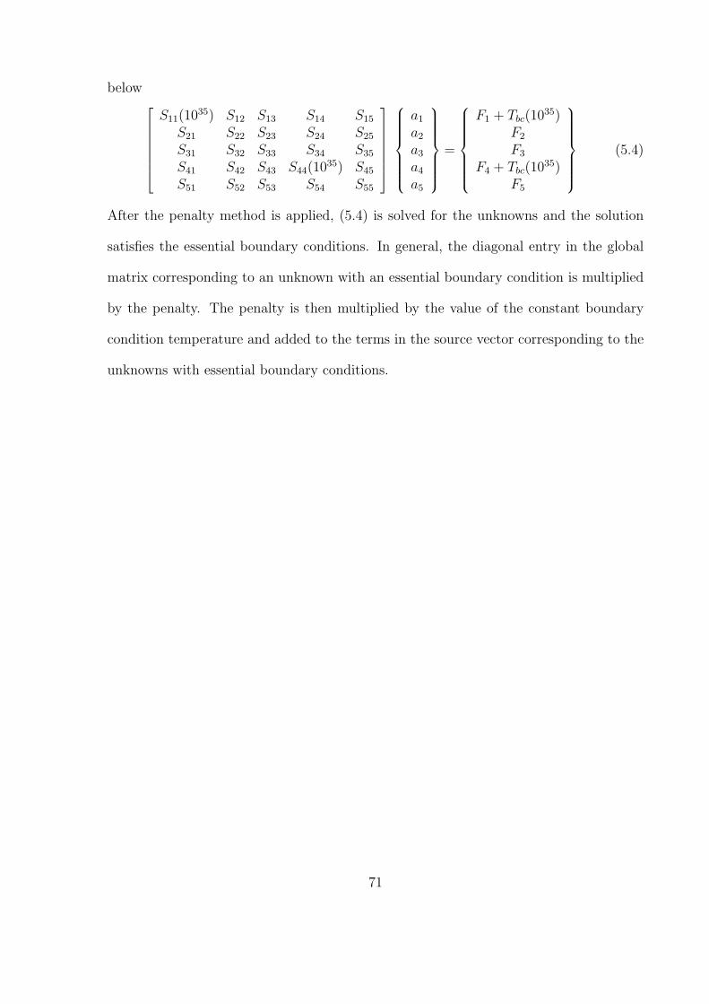
below

S11(1035) S12 S13 S14 S15

S21 S22 S23 S24 S25

S31 S32 S33 S34 S35

S41 S42 S43 S44(1035) S45

S51 S52 S53 S54 S55

a1

a2

a3

a4

a5

=

F1 + Tbc(1035)F2

F3

F4 + Tbc(1035)F5

(5.4)

After the penalty method is applied, (5.4) is solved for the unknowns and the solution

satisfies the essential boundary conditions. In general, the diagonal entry in the global

matrix corresponding to an unknown with an essential boundary condition is multiplied

by the penalty. The penalty is then multiplied by the value of the constant boundary

condition temperature and added to the terms in the source vector corresponding to the

unknowns with essential boundary conditions.

71

Chapter 6

Numerical Results

After the finite element approximation is calculated, the accuracy of the approximation

must be determined. In this chapter, the methods used to quantify the error are discussed.

This discussion is followed by several sample problems and an error analysis of each

problem.

6.1 Error Convergence Estimates

In order to determine the accuracy of the finite element method presented, an effective

way of quantifying the error in the approximation is needed. There are two types of error

estimates used to quantify the error, a priori and a posteriori. A priori error estimates

give the theoretical rate of convergence of the error and are based on the exact solution to

a problem. A posteriori error estimates use the finite element solution to a problem since

the exact solution is usually not known. In this research, the rate of error convergence

for the approximation is compared to a priori error convergence estimates.

The error in the approximation at any point is defined as

e (x, y, z, t) = u (x, y, z, t)− u (x, y, z, t) (6.1)

where u is the exact solution and u is the approximate solution. The error analysis in

this research utilizes H1 norms in space and L2 norms in time. The H1, or energy norm,

72

quantifies the spatial error in the finite element approximation

‖ e (t) ‖H1(Ω) =

∫

Ω

e2 +

(∂e

∂x

)2

+

(∂e

∂y

)2

+

(∂e

∂z

)2 dx dy dz

12

(6.2)

This error norm is a function of time. By evaluating (6.2) at a particular point in time,

the global error in space at any point in time can be determined. The global error in

space and time is calculated by taking the L2 norm of (6.2) with respect to time

‖ e ‖L2(I,H1(Ω)) =

[∫ T

0‖ e (t) ‖2

H1(Ω) dt

] 12

(6.3)

=

∫ T

0

∫

Ω

e2 +

(∂e

∂x

)2

+

(∂e

∂y

)2

+

(∂e

∂z

)2 dx dy dz

dt

12

where I denotes the entire time interval, (0, T ], and H1(Ω) represents the spatial error

norm. The L2 norm is also known as the root mean square norm because it is analogous

to the root mean square error at a point. The difference is that the L2 norm is used for

the error between two functions, not two points. The global error over the entire time

interval is given by (6.3). For multiple time steps, the error norm is calculated at each

time step

‖ e ‖L2(In,H1(Ω))=

∫ tn

tn−1

∫

Ω

e2 +

(∂e

∂x

)2

+

(∂e

∂y

)2

+

(∂e

∂z

)2 dx dy dz

dt

12

(6.4)

and the total global error norm is the sum of the error norms from each time step

‖ e ‖L2(I,H1(Ω))=

[nt∑

1

‖ e ‖2L2(In,H1(Ω))

] 12

(6.5)

One issue with the H1 and L2 norms is that the magnitude depends on the magnitude

of the exact solution. This means that the value of the global error has little meaning

without the magnitude of the exact solution. In order to remedy this, the magnitude of

the H1 and L2 norms of the exact solution are calculated for each problem. Using the

magnitude of the exact solution norms, the H1 and L2 error norms can be normalized

73

and the percent error in the H1 and L2 norms calculated

% error in H1(Ω) = 100

( ‖ e (t) ‖H1(Ω)

‖ u (t) ‖H1(Ω)

)(6.6)

% error in L2(I, H1(Ω)

)= 100

( ‖ e ‖L2(I,H1(Ω))

‖ u ‖L2(I,H1(Ω))

)(6.7)

For a priori error estimates, the rate convergence of the error in an approximation is

known prior to the calculation of the approximation. The error for the in-plane, through-

thickness, and time approximations are dependent on the degree of the approximation and

the mesh size [27]. Work by Schotzau and Schwab [16] and Werder, et al. [26] established

the error bounds for linear, transient heat conduction problems. The error bounds assume

a uniform mesh size and uniform degrees of approximation for all of the elements. For

an approximation where the only source of error is the in-plane approximation, the H1

norm of the error is bounded by

‖ e (t) ‖H1(Ω)≤ C1hpip (6.8)

where C1 is a constant, h is the size of an in-plane element, and pip is the degree of the

in-plane approximation. As the size of an element is decreased, the H1 error converges

to zero at a rate of pip. For an approximation where the only source of error is the

approximation in time, the L2 norm of the error is bounded by

‖ e ‖L2(I,H1(Ω))≤ C2∆tpt+1 (6.9)

where C2 is a constant, ∆t is size of the uniform time step, and pt is the degree of the

time approximation. As the size of the time step is decreased, the L2 error converges

to zero at a rate of pt + 1. Since the size of the time step is inversely proportional to

the number of time steps, this means that as the number of time steps increases, the L2

error converges to zero at a rate of pt +1. In (6.8) and (6.9), the in-plane and time error,

74

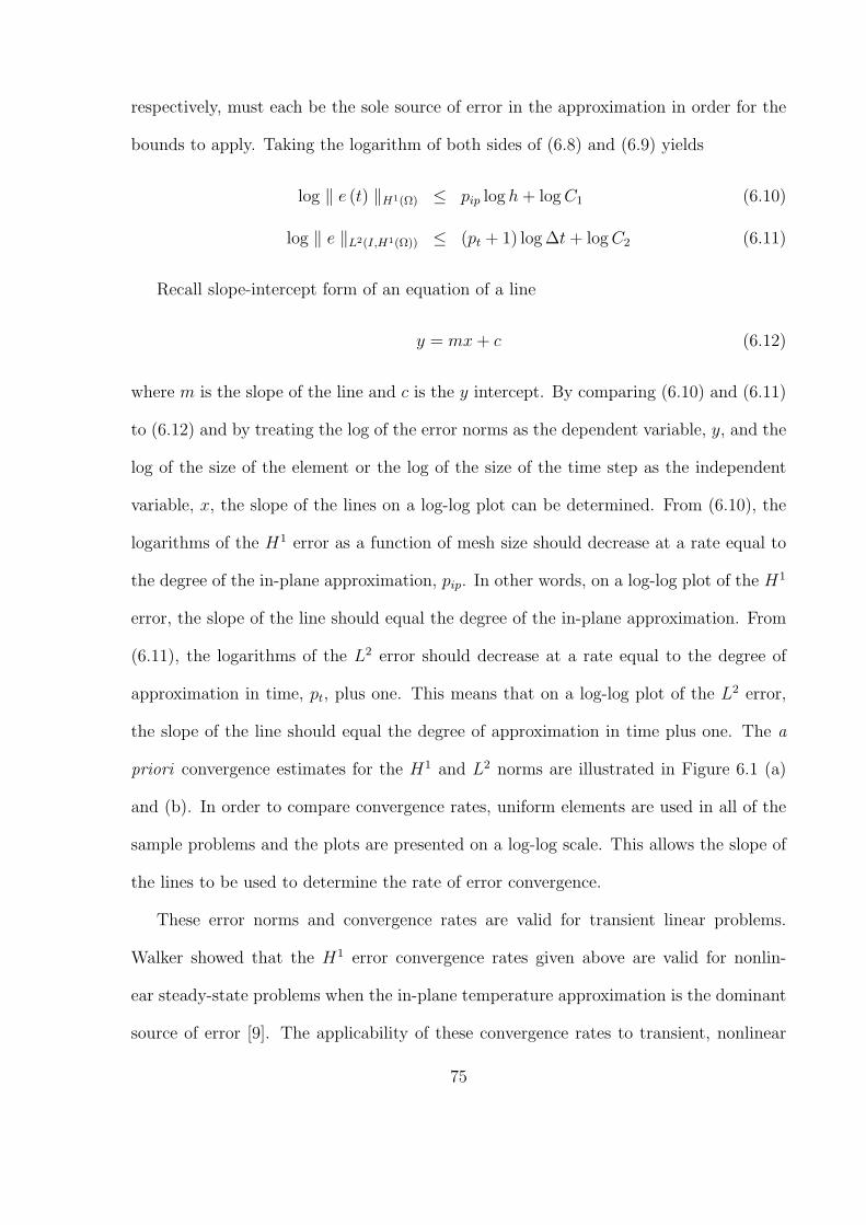
respectively, must each be the sole source of error in the approximation in order for the

bounds to apply. Taking the logarithm of both sides of (6.8) and (6.9) yields

log ‖ e (t) ‖H1(Ω) ≤ pip log h + log C1 (6.10)

log ‖ e ‖L2(I,H1(Ω)) ≤ (pt + 1) log ∆t + log C2 (6.11)

Recall slope-intercept form of an equation of a line

y = mx + c (6.12)

where m is the slope of the line and c is the y intercept. By comparing (6.10) and (6.11)

to (6.12) and by treating the log of the error norms as the dependent variable, y, and the

log of the size of the element or the log of the size of the time step as the independent

variable, x, the slope of the lines on a log-log plot can be determined. From (6.10), the

logarithms of the H1 error as a function of mesh size should decrease at a rate equal to

the degree of the in-plane approximation, pip. In other words, on a log-log plot of the H1

error, the slope of the line should equal the degree of the in-plane approximation. From

(6.11), the logarithms of the L2 error should decrease at a rate equal to the degree of

approximation in time, pt, plus one. This means that on a log-log plot of the L2 error,

the slope of the line should equal the degree of approximation in time plus one. The a

priori convergence estimates for the H1 and L2 norms are illustrated in Figure 6.1 (a)

and (b). In order to compare convergence rates, uniform elements are used in all of the

sample problems and the plots are presented on a log-log scale. This allows the slope of

the lines to be used to determine the rate of error convergence.

These error norms and convergence rates are valid for transient linear problems.

Walker showed that the H1 error convergence rates given above are valid for nonlin-

ear steady-state problems when the in-plane temperature approximation is the dominant

source of error [9]. The applicability of these convergence rates to transient, nonlinear

75

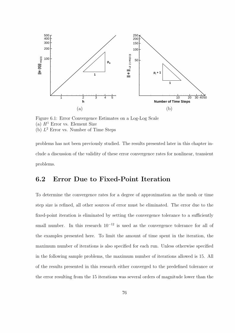
h

||e(t

)|| H

1(Ω

)

1 2 3 4 5

100

200

300400500

1

pip

(a)

Number of Time Steps

||e

||L

2(

I;H

1(Ω

))

10 20 30 4050

50

100

150200250

1

pt + 1

(b)

Figure 6.1: Error Convergence Estimates on a Log-Log Scale(a) H1 Error vs. Element Size(b) L2 Error vs. Number of Time Steps

problems has not been previously studied. The results presented later in this chapter in-

clude a discussion of the validity of these error convergence rates for nonlinear, transient

problems.

6.2 Error Due to Fixed-Point Iteration

To determine the convergence rates for a degree of approximation as the mesh or time

step size is refined, all other sources of error must be eliminated. The error due to the

fixed-point iteration is eliminated by setting the convergence tolerance to a sufficiently

small number. In this research 10−12 is used as the convergence tolerance for all of

the examples presented here. To limit the amount of time spent in the iteration, the

maximum number of iterations is also specified for each run. Unless otherwise specified

in the following sample problems, the maximum number of iterations allowed is 15. All

of the results presented in this research either converged to the predefined tolerance or

the error resulting from the 15 iterations was several orders of magnitude lower than the

76

error in the solution.

For real world applications, an iteration tolerance of 10−12 is not practical or necessary.

For practical purposes, convergence to a tenth or hundredth of a degree is adequate. This

accuracy is normally obtained by ndgSCHTp within three or four iterations.

6.3 Sample Problems

For most nonlinear, transient problems of conduction heat transfer, an exact solution

to the initial boundary value problem is impossible to determine. In order to precisely

analyze the accuracy of the method, problems with exact solutions are created so that the

exact error can be computed. Since the initial and boundary conditions are determined

directly from the exact solution, an exact solution with appropriate initial and boundary

conditions should be chosen. To construct a problem with an exact solution, u, the source

term for the problem, Q, is obtained by substituting u into (2.1)

Q = ρcp∂u

∂t− k(u)

(∂2u

∂x2+

∂2u

∂y2+

∂2u

∂z2

)− ∂k(u)

∂x

∂u

∂x− ∂k(u)

∂y

∂u

∂y− ∂k(u)

∂z

∂u

∂z(6.13)

A function for the thermal conductivity is also chosen. In the examples presented in this

research, the thermal conductivity is restricted to be a polynomial function of tempera-

ture of the form

k(u) = Ckum + k0 (6.14)

where Ck and k0 are constants and m is an integer exponent. Substituting (6.14) into

(6.13) and simplifying yields

Q = ρcp∂u

∂t− (Cku

m + k0)

(∂2u

∂x2+

∂2u

∂y2+

∂2u

∂z2

)

−mCkum−1

(∂u

∂x

)2

+

(∂u

∂y

)2

+

(∂u

∂z

)2 (6.15)

If the exact solution and thermal conductivity are chosen to be simple polynomials,

then ndgSCHTp should produce the exact solution when the polynomial degree of the

77

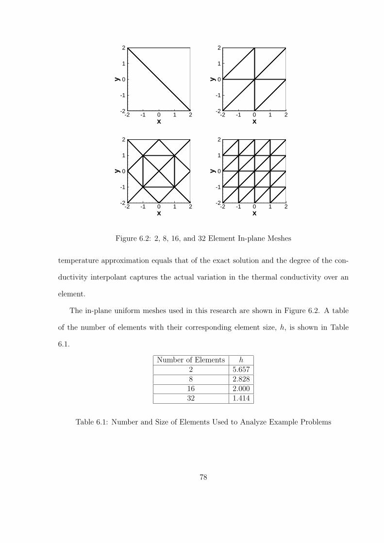
xy

-2 -1 0 1 2-2

-1

0

1

2

x

y

-2 -1 0 1 2-2

-1

0

1

2

x

y

-2 -1 0 1 2-2

-1

0

1

2

xy

-2 -1 0 1 2-2

-1

0

1

2

Figure 6.2: 2, 8, 16, and 32 Element In-plane Meshes

temperature approximation equals that of the exact solution and the degree of the con-

ductivity interpolant captures the actual variation in the thermal conductivity over an

element.

The in-plane uniform meshes used in this research are shown in Figure 6.2. A table

of the number of elements with their corresponding element size, h, is shown in Table

6.1.

Number of Elements h2 5.6578 2.82816 2.00032 1.414

Table 6.1: Number and Size of Elements Used to Analyze Example Problems

78

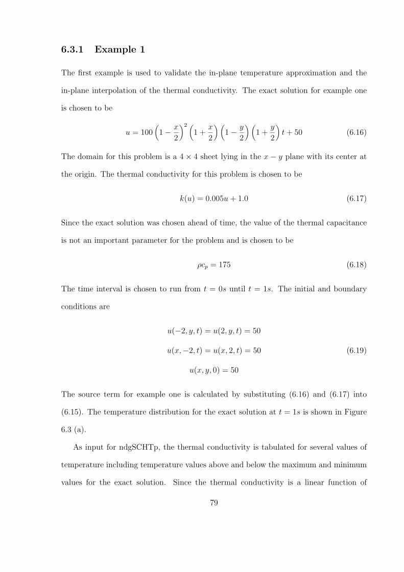
6.3.1 Example 1

The first example is used to validate the in-plane temperature approximation and the

in-plane interpolation of the thermal conductivity. The exact solution for example one

is chosen to be

u = 100(1− x

2

)2 (1 +

x

2

) (1− y

2

) (1 +

y

2

)t + 50 (6.16)

The domain for this problem is a 4× 4 sheet lying in the x− y plane with its center at

the origin. The thermal conductivity for this problem is chosen to be

k(u) = 0.005u + 1.0 (6.17)

Since the exact solution was chosen ahead of time, the value of the thermal capacitance

is not an important parameter for the problem and is chosen to be

ρcp = 175 (6.18)

The time interval is chosen to run from t = 0s until t = 1s. The initial and boundary

conditions are

u(−2, y, t) = u(2, y, t) = 50

u(x,−2, t) = u(x, 2, t) = 50 (6.19)

u(x, y, 0) = 50

The source term for example one is calculated by substituting (6.16) and (6.17) into

(6.15). The temperature distribution for the exact solution at t = 1s is shown in Figure

6.3 (a).

As input for ndgSCHTp, the thermal conductivity is tabulated for several values of

temperature including temperature values above and below the maximum and minimum

values for the exact solution. Since the thermal conductivity is a linear function of

79

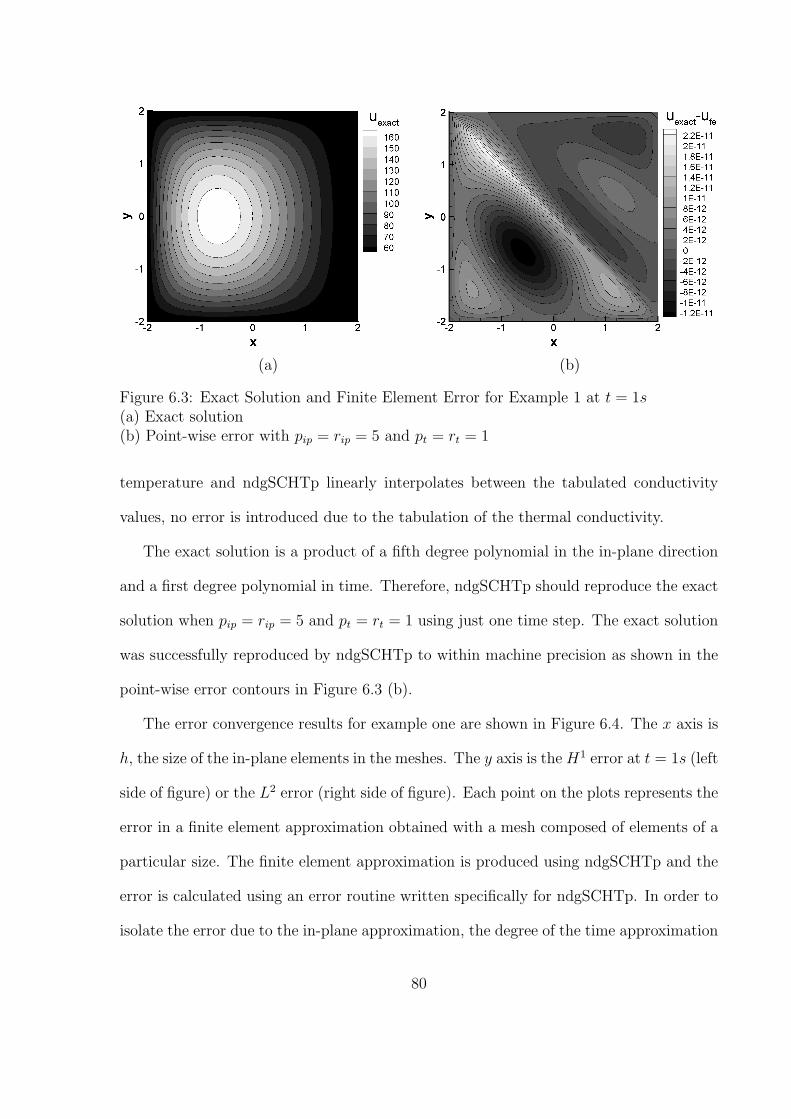
(a) (b)

Figure 6.3: Exact Solution and Finite Element Error for Example 1 at t = 1s(a) Exact solution(b) Point-wise error with pip = rip = 5 and pt = rt = 1

temperature and ndgSCHTp linearly interpolates between the tabulated conductivity

values, no error is introduced due to the tabulation of the thermal conductivity.

The exact solution is a product of a fifth degree polynomial in the in-plane direction

and a first degree polynomial in time. Therefore, ndgSCHTp should reproduce the exact

solution when pip = rip = 5 and pt = rt = 1 using just one time step. The exact solution

was successfully reproduced by ndgSCHTp to within machine precision as shown in the

point-wise error contours in Figure 6.3 (b).

The error convergence results for example one are shown in Figure 6.4. The x axis is

h, the size of the in-plane elements in the meshes. The y axis is the H1 error at t = 1s (left

side of figure) or the L2 error (right side of figure). Each point on the plots represents the

error in a finite element approximation obtained with a mesh composed of elements of a

particular size. The finite element approximation is produced using ndgSCHTp and the

error is calculated using an error routine written specifically for ndgSCHTp. In order to

isolate the error due to the in-plane approximation, the degree of the time approximation

80

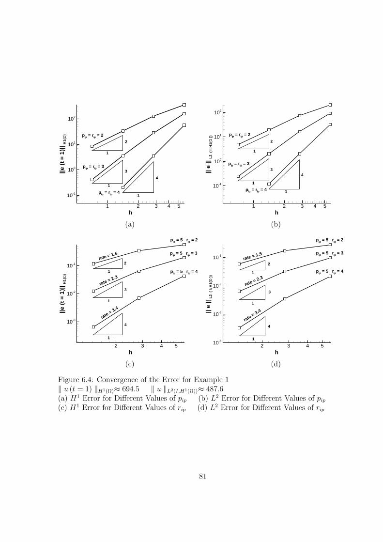
h

||e(t

=1

)|| H

1(Ω

)

1 2 3 4 5

10-1

100

101

102

pip = rip = 2

pip = rip = 3

pip = rip = 4

1

1

1

2

3

4

(a)

h||

e||

L2

(I;

H1(

Ω))

1 2 3 4 5

10-1

100

101

102

1

1

1

2

34

pip = rip = 3

pip = rip = 2

pip = rip = 4

(b)

h

||e(t

=1

)|| H

1(Ω

)

2 3 4 5

10-3

10-2

10-1

pip = 5 rip = 3

pip = 5 rip = 4

pip = 5 rip = 2

1

1

1

4

3

2rate = 1.5

rate = 2.3

rate= 3.4

(c)

h

||e

||L

2(

I;H

1(Ω

))

2 3 4 510-4

10-3

10-2

10-1

pip = 5 rip = 4

pip = 5 rip = 2

pip = 5 rip = 3

1

1

1

2

3

4

rate = 1.5

rate = 2.3

rate= 3.4

(d)

Figure 6.4: Convergence of the Error for Example 1‖ u (t = 1) ‖H1(Ω)≈ 694.5 ‖ u ‖L2(I,H1(Ω))≈ 487.6(a) H1 Error for Different Values of pip (b) L2 Error for Different Values of pip

(c) H1 Error for Different Values of rip (d) L2 Error for Different Values of rip

81

and interpolation was set equal to that of the exact solution, pt = rt = 1. This makes the

finite element approximation exact in time. Since there is no error in time, the in-plane

temperature approximation and conductivity interpolation are the only sources of error

in the finite element approximation.

In Figure 6.4, each line represents a finite element approximation with a particular

value for the degree of in-plane temperature approximation, pip, and the degree of in-

plane conductivity interpolation, rip. Each point on a line represents the error for a given

size mesh. As the number of elements in the mesh is increased, the size of the element,

h, decreases. The error convergence rates for linear problems, discussed earlier in this

chapter, are compared to the convergence rates obtained for this nonlinear problem.

In Figure 6.4 (a), the H1 error versus mesh size at t = 1s is shown on a log-log scale.

Each line represents a different value for pip. The in-plane interpolation degree, rip, is

set equal to the in-plane temperature approximation degree, pip. The triangles show

the theoretical rates of convergence for linear problems. The convergence rates for this

nonlinear example are identical to the convergence rates expected for a linear problem.

In Figure 6.4 (b), the L2 error versus mesh size is shown on a log-log scale for varying

in-plane degrees of temperature approximation. The L2 error is a representation of the

total error including the secondary variables in space over the entire time interval for the

problem. The convergence rates for the L2 error should be the same as the convergence

rates for the H1 error since the L2 error takes into account the H1 error in space. Again,

the expected convergence rates for the linear problem are achieved for this nonlinear

problem. The triangles in the figure have the same slope as the lines.

In Figure 6.4 (c) and Figure 6.4 (d), the H1 error at t = 1s and the L2 error versus

mesh size are shown on a log-log scale. Each line represents a different value for rip with

pip = 5, the degree of the exact solution. This isolates the in-plane interpolation of the

82

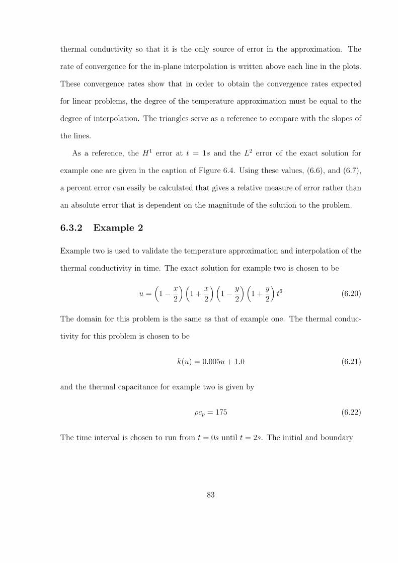
thermal conductivity so that it is the only source of error in the approximation. The

rate of convergence for the in-plane interpolation is written above each line in the plots.

These convergence rates show that in order to obtain the convergence rates expected

for linear problems, the degree of the temperature approximation must be equal to the

degree of interpolation. The triangles serve as a reference to compare with the slopes of

the lines.

As a reference, the H1 error at t = 1s and the L2 error of the exact solution for

example one are given in the caption of Figure 6.4. Using these values, (6.6), and (6.7),

a percent error can easily be calculated that gives a relative measure of error rather than

an absolute error that is dependent on the magnitude of the solution to the problem.

6.3.2 Example 2

Example two is used to validate the temperature approximation and interpolation of the

thermal conductivity in time. The exact solution for example two is chosen to be

u =(1− x

2

) (1 +

x

2

) (1− y

2

) (1 +

y

2

)t6 (6.20)

The domain for this problem is the same as that of example one. The thermal conduc-

tivity for this problem is chosen to be

k(u) = 0.005u + 1.0 (6.21)

and the thermal capacitance for example two is given by

ρcp = 175 (6.22)

The time interval is chosen to run from t = 0s until t = 2s. The initial and boundary

83

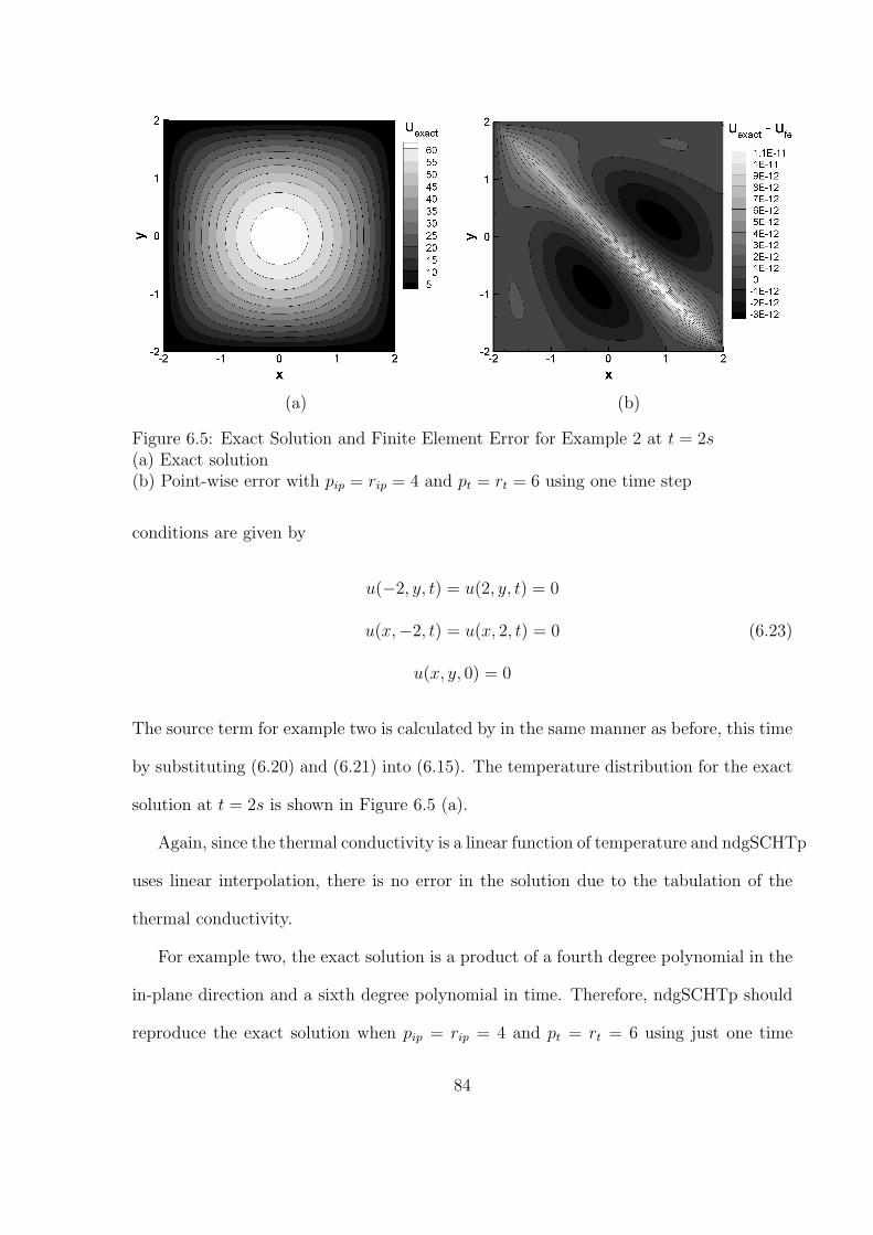
(a) (b)

Figure 6.5: Exact Solution and Finite Element Error for Example 2 at t = 2s(a) Exact solution(b) Point-wise error with pip = rip = 4 and pt = rt = 6 using one time step

conditions are given by

u(−2, y, t) = u(2, y, t) = 0

u(x,−2, t) = u(x, 2, t) = 0 (6.23)

u(x, y, 0) = 0

The source term for example two is calculated by in the same manner as before, this time

by substituting (6.20) and (6.21) into (6.15). The temperature distribution for the exact

solution at t = 2s is shown in Figure 6.5 (a).

Again, since the thermal conductivity is a linear function of temperature and ndgSCHTp

uses linear interpolation, there is no error in the solution due to the tabulation of the

thermal conductivity.

For example two, the exact solution is a product of a fourth degree polynomial in the

in-plane direction and a sixth degree polynomial in time. Therefore, ndgSCHTp should

reproduce the exact solution when pip = rip = 4 and pt = rt = 6 using just one time

84

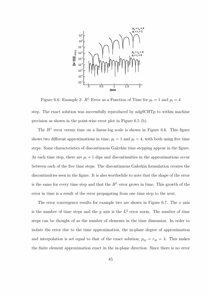
time

||e(t

)|| H

1(Ω

)

0 0.5 1 1.5 210-7

10-6

10-5

10-4

10-3

10-2

10-1

100

101

pip = rip = 4pt = rt = 4

pip = rip = 4pt = rt = 1

Figure 6.6: Example 2: H1 Error as a Function of Time for pt = 1 and pt = 4

step. The exact solution was successfully reproduced by ndgSCHTp to within machine

precision as shown in the point-wise error plot in Figure 6.5 (b).

The H1 error versus time on a linear-log scale is shown in Figure 6.6. This figure

shows two different approximations in time, pt = 1 and pt = 4, with both using five time

steps. Some characteristics of discontinuous Galerkin time stepping appear in the figure.

At each time step, there are pt + 1 dips and discontinuities in the approximations occur

between each of the five time steps. The discontinuous Galerkin formulation creates the

discontinuities seen in the figure. It is also worthwhile to note that the shape of the error

is the same for every time step and that the H1 error grows in time. This growth of the

error in time is a result of the error propagating from one time step to the next.

The error convergence results for example two are shown in Figure 6.7. The x axis

is the number of time steps and the y axis is the L2 error norm. The number of time

steps can be thought of as the number of elements in the time dimension. In order to

isolate the error due to the time approximation, the in-plane degree of approximation

and interpolation is set equal to that of the exact solution, pip = rip = 4. This makes

the finite element approximation exact in the in-plane direction. Since there is no error

85

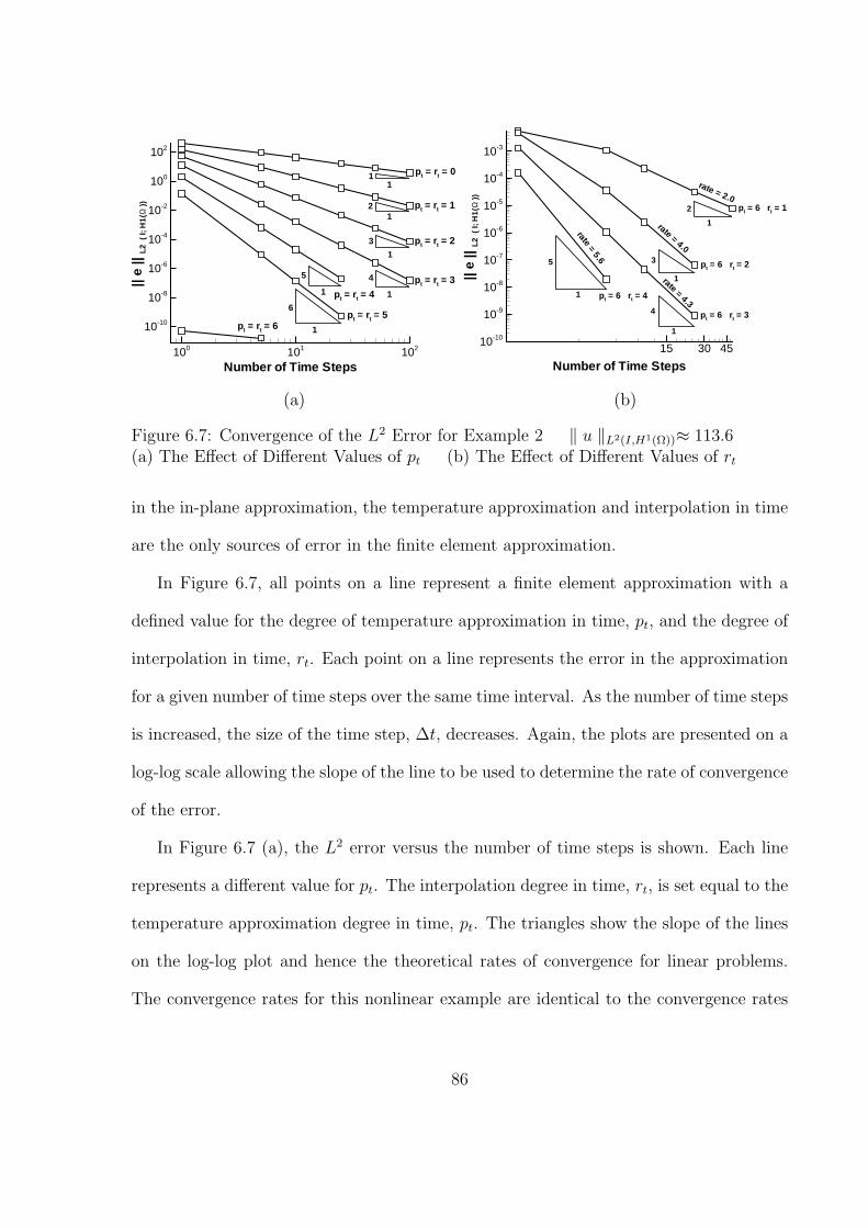
Number of Time Steps

||e

||L2

(I;

H1

(Ω))

100 101 102

10-10

10-8

10-6

10-4

10-2

100

102

pt = rt = 4

pt = rt = 1

pt = rt = 2

pt = rt = 3

pt = rt = 6

pt = rt = 01

1

1

11

1

1

2

3

45

6pt = rt = 5

(a)

Number of Time Steps

||e

||L2

(I;

H1(

Ω))

15 30 4510-10

10-9

10-8

10-7

10-6

10-5

10-4

10-3

1

1

1

1

2

3

4

5

pt = 6 rt = 4

pt = 6 rt = 1

pt = 6 rt = 2

pt = 6 rt = 3

rate=

5.6

rate = 2.0

rate = 4.0

rate =4.3

(b)

Figure 6.7: Convergence of the L2 Error for Example 2 ‖ u ‖L2(I,H1(Ω))≈ 113.6(a) The Effect of Different Values of pt (b) The Effect of Different Values of rt

in the in-plane approximation, the temperature approximation and interpolation in time

are the only sources of error in the finite element approximation.

In Figure 6.7, all points on a line represent a finite element approximation with a

defined value for the degree of temperature approximation in time, pt, and the degree of

interpolation in time, rt. Each point on a line represents the error in the approximation

for a given number of time steps over the same time interval. As the number of time steps

is increased, the size of the time step, ∆t, decreases. Again, the plots are presented on a

log-log scale allowing the slope of the line to be used to determine the rate of convergence

of the error.

In Figure 6.7 (a), the L2 error versus the number of time steps is shown. Each line

represents a different value for pt. The interpolation degree in time, rt, is set equal to the

temperature approximation degree in time, pt. The triangles show the slope of the lines

on the log-log plot and hence the theoretical rates of convergence for linear problems.

The convergence rates for this nonlinear example are identical to the convergence rates

86

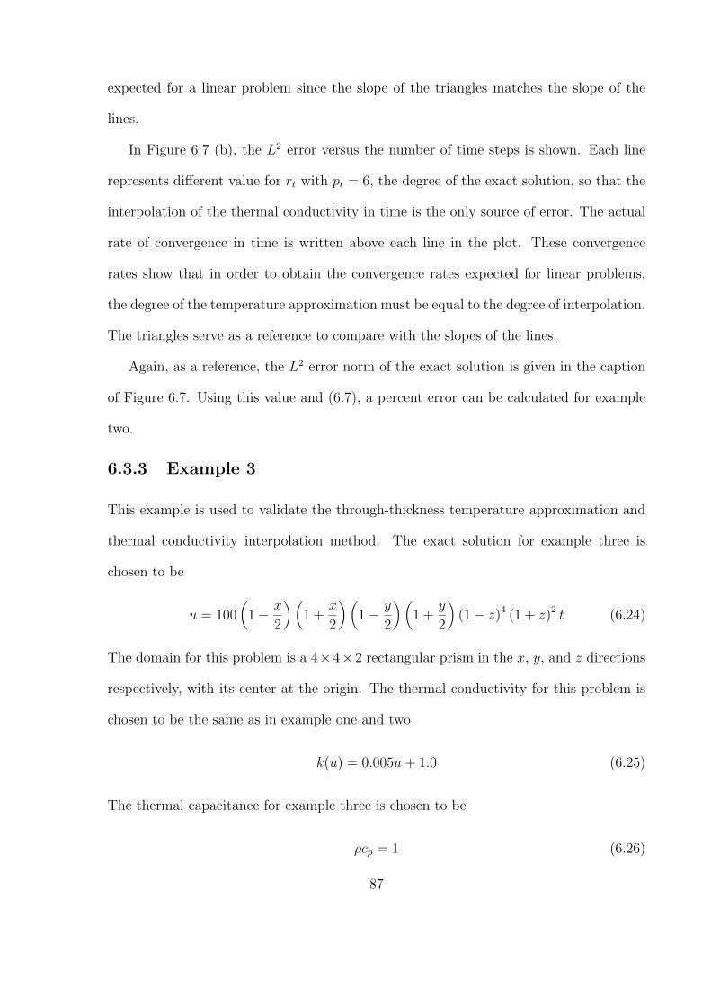
expected for a linear problem since the slope of the triangles matches the slope of the

lines.

In Figure 6.7 (b), the L2 error versus the number of time steps is shown. Each line

represents different value for rt with pt = 6, the degree of the exact solution, so that the

interpolation of the thermal conductivity in time is the only source of error. The actual

rate of convergence in time is written above each line in the plot. These convergence

rates show that in order to obtain the convergence rates expected for linear problems,

the degree of the temperature approximation must be equal to the degree of interpolation.

The triangles serve as a reference to compare with the slopes of the lines.

Again, as a reference, the L2 error norm of the exact solution is given in the caption

of Figure 6.7. Using this value and (6.7), a percent error can be calculated for example

two.

6.3.3 Example 3

This example is used to validate the through-thickness temperature approximation and

thermal conductivity interpolation method. The exact solution for example three is

chosen to be

u = 100(1− x

2

) (1 +

x

2

) (1− y

2

) (1 +

y

2

)(1− z)4 (1 + z)2 t (6.24)

The domain for this problem is a 4×4×2 rectangular prism in the x, y, and z directions

respectively, with its center at the origin. The thermal conductivity for this problem is

chosen to be the same as in example one and two

k(u) = 0.005u + 1.0 (6.25)

The thermal capacitance for example three is chosen to be

ρcp = 1 (6.26)

87

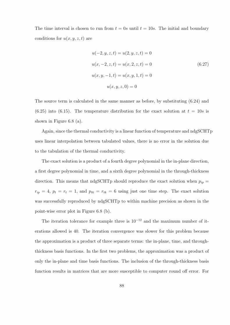
The time interval is chosen to run from t = 0s until t = 10s. The initial and boundary

conditions for u(x, y, z, t) are

u(−2, y, z, t) = u(2, y, z, t) = 0

u(x,−2, z, t) = u(x, 2, z, t) = 0 (6.27)

u(x, y,−1, t) = u(x, y, 1, t) = 0

u(x, y, z, 0) = 0

The source term is calculated in the same manner as before, by substituting (6.24) and

(6.25) into (6.15). The temperature distribution for the exact solution at t = 10s is

shown in Figure 6.8 (a).

Again, since the thermal conductivity is a linear function of temperature and ndgSCHTp

uses linear interpolation between tabulated values, there is no error in the solution due

to the tabulation of the thermal conductivity.

The exact solution is a product of a fourth degree polynomial in the in-plane direction,

a first degree polynomial in time, and a sixth degree polynomial in the through-thickness

direction. This means that ndgSCHTp should reproduce the exact solution when pip =

rip = 4, pt = rt = 1, and ptk = rtk = 6 using just one time step. The exact solution

was successfully reproduced by ndgSCHTp to within machine precision as shown in the

point-wise error plot in Figure 6.8 (b).

The iteration tolerance for example three is 10−12 and the maximum number of it-

erations allowed is 40. The iteration convergence was slower for this problem because

the approximation is a product of three separate terms: the in-plane, time, and through-

thickness basis functions. In the first two problems, the approximation was a product of

only the in-plane and time basis functions. The inclusion of the through-thickness basis

function results in matrices that are more susceptible to computer round off error. For

88

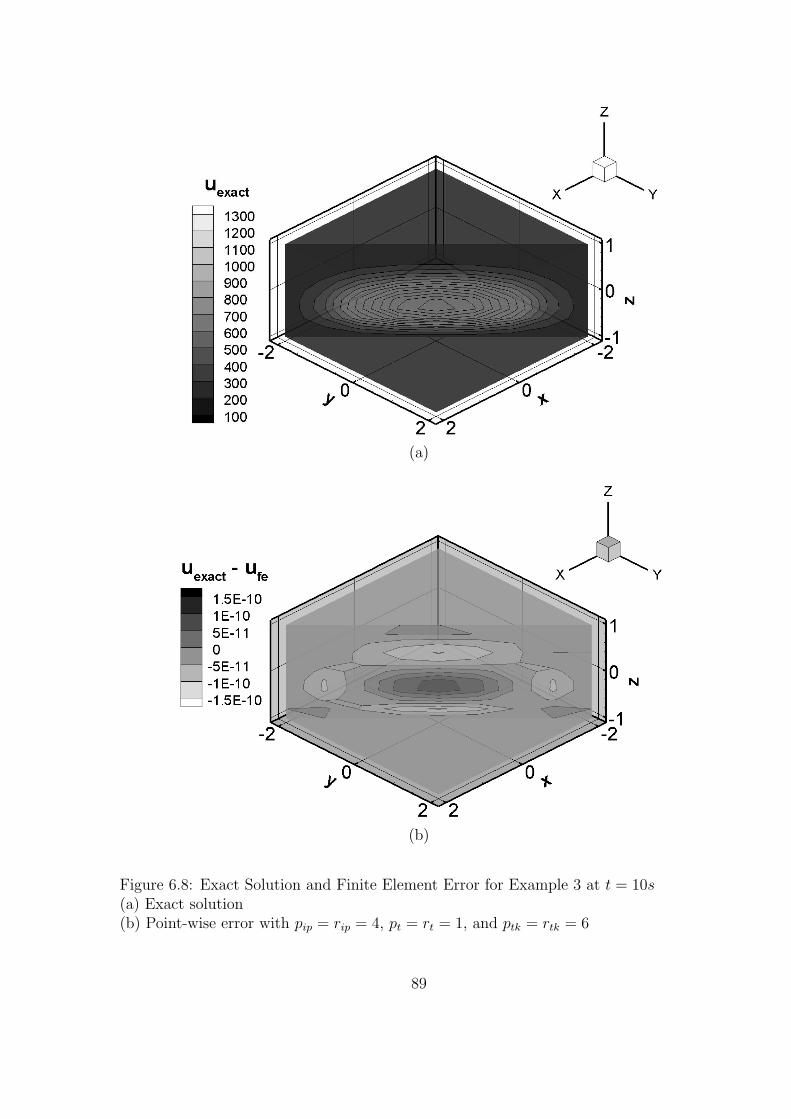
(a)

(b)

Figure 6.8: Exact Solution and Finite Element Error for Example 3 at t = 10s(a) Exact solution(b) Point-wise error with pip = rip = 4, pt = rt = 1, and ptk = rtk = 6

89

this example, iteration convergence to less than a tenth of a degree is achieved within

five or six iterations.

The error convergence results for example three are shown in Figure 6.9. In (a), (b),

(c), and (d) the x axis is h, the size of an in-plane element, and the y axis is the H1

error norm at t = 10s or the L2 error norm. In order to isolate the error due to the in-

plane and through-thickness approximations, the degree of the time approximation and

interpolation was set equal to that of the exact solution, pt = rt = 1. The finite element

approximation is then exact in time. Since there is no error in time, the in-plane and

through-thickness temperature approximations and interpolations are the only sources

of error in the finite element approximation.

In Figure 6.9 (a), the H1 error versus the size of an in-plane element at t = 10s is

shown on a log-log scale. Each line represents different value for pip. In order to isolate the

error due to the in-plane approximation, the degree of through-thickness approximation

and interpolation was set equal to that of the exact solution, ptk = rtk = 6. The in-plane

interpolation degree, rip, is set equal to the in-plane temperature approximation degree,

pip. The convergence rates for the in-plane approximation are either equal to or slightly

better than the convergence rates expected for a linear problem. In Figure 6.9 (b), the

L2 error versus h on a log-log scale is shown for varying in-plane degrees of temperature

approximation. Again, the achieved convergence rates are either equal to or slightly

better than the convergence rates expected for a linear problem.

In Figure 6.9 (c) and Figure 6.9 (d), the H1 error at t = 10s and the L2 error versus

h are shown on a log-log scale. The in-plane degree of temperature approximation and

interpolation are set equal to three in both plots. Each line represents a different value

for ptk with rtk = ptk. There is no mesh refinement in the through-thickness direction

since the finite element method collapsed the through-thickness approximation onto the

90

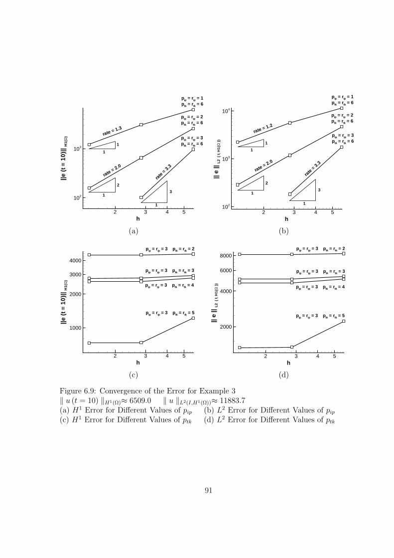
h

||e(t

=1

0)||

H1

(Ω)

2 3 4 5

102

103

pip = rip = 3ptk = rtk = 6

pip = rip = 1ptk = rtk = 6

pip = rip = 2ptk = rtk = 6

1

1

1

3

2

1

rate = 1.3

rate

=3.3

rate = 2.0

(a)

h||

e||

L2

(I;

H1(

Ω))

2 3 4 5102

103

104

pip = rip = 3ptk = rtk = 6

pip = rip = 1ptk = rtk = 6

pip = rip = 2ptk = rtk = 6

1

1

1

1

3

2

rate = 1.2

rate = 2.0

rate

= 3.3

(b)

h

||e(t

=1

0)||

H1(

Ω)

2 3 4 5

1000

2000

3000

4000

pip = rip = 3 ptk = rtk = 5

pip = rip = 3 ptk = rtk = 2

pip = rip = 3 ptk = rtk = 3

pip = rip = 3 ptk = rtk = 4

(c)

h

||e

||L

2(

I;H

1(Ω

))

2 3 4 5

2000

4000

6000

8000

pip = rip = 3 ptk = rtk = 5

pip = rip = 3 ptk = rtk = 2

pip = rip = 3 ptk = rtk = 3

pip = rip = 3 ptk = rtk = 4

(d)

Figure 6.9: Convergence of the Error for Example 3‖ u (t = 10) ‖H1(Ω)≈ 6509.0 ‖ u ‖L2(I,H1(Ω))≈ 11883.7(a) H1 Error for Different Values of pip (b) L2 Error for Different Values of pip

(c) H1 Error for Different Values of ptk (d) L2 Error for Different Values of ptk

91

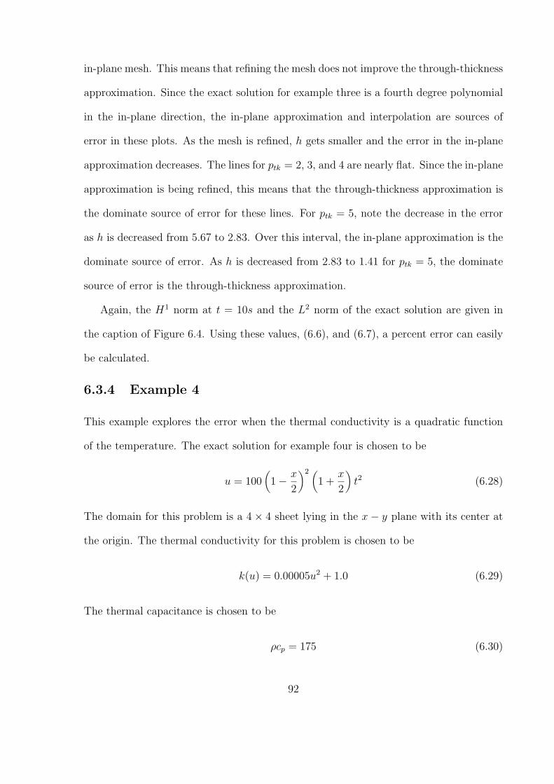
in-plane mesh. This means that refining the mesh does not improve the through-thickness

approximation. Since the exact solution for example three is a fourth degree polynomial

in the in-plane direction, the in-plane approximation and interpolation are sources of

error in these plots. As the mesh is refined, h gets smaller and the error in the in-plane

approximation decreases. The lines for ptk = 2, 3, and 4 are nearly flat. Since the in-plane

approximation is being refined, this means that the through-thickness approximation is

the dominate source of error for these lines. For ptk = 5, note the decrease in the error

as h is decreased from 5.67 to 2.83. Over this interval, the in-plane approximation is the

dominate source of error. As h is decreased from 2.83 to 1.41 for ptk = 5, the dominate

source of error is the through-thickness approximation.

Again, the H1 norm at t = 10s and the L2 norm of the exact solution are given in

the caption of Figure 6.4. Using these values, (6.6), and (6.7), a percent error can easily

be calculated.

6.3.4 Example 4

This example explores the error when the thermal conductivity is a quadratic function

of the temperature. The exact solution for example four is chosen to be

u = 100(1− x

2

)2 (1 +

x

2

)t2 (6.28)

The domain for this problem is a 4× 4 sheet lying in the x− y plane with its center at

the origin. The thermal conductivity for this problem is chosen to be

k(u) = 0.00005u2 + 1.0 (6.29)

The thermal capacitance is chosen to be

ρcp = 175 (6.30)

92

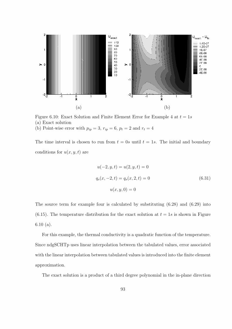
(a) (b)

Figure 6.10: Exact Solution and Finite Element Error for Example 4 at t = 1s(a) Exact solution(b) Point-wise error with pip = 3, rip = 6, pt = 2 and rt = 4

The time interval is chosen to run from t = 0s until t = 1s. The initial and boundary

conditions for u(x, y, t) are

u(−2, y, t) = u(2, y, t) = 0

qs(x,−2, t) = qs(x, 2, t) = 0 (6.31)

u(x, y, 0) = 0

The source term for example four is calculated by substituting (6.28) and (6.29) into

(6.15). The temperature distribution for the exact solution at t = 1s is shown in Figure

6.10 (a).

For this example, the thermal conductivity is a quadratic function of the temperature.

Since ndgSCHTp uses linear interpolation between the tabulated values, error associated

with the linear interpolation between tabulated values is introduced into the finite element

approximation.

The exact solution is a product of a third degree polynomial in the in-plane direction

93

and a second degree polynomial in time. Since the thermal conductivity is a quadratic

function of temperature, the interpolation used to account for the temperature-dependent

thermal conductivity must reflect its quadratic dependence on the temperature. To

accurately capture the quadratic variation in the thermal conductivity as a function

of temperature, the degrees of interpolation should be twice the degrees of the exact

temperature approximation. Then the only error in the finite element approximation is

the error associated with the linear interpolation between the tabulated values of the

thermal conductivity. By tabulating the values of thermal conductivity every quarter of

a degree, this error can be minimized. Therefore, ndgSCHTp should nearly reproduce

the exact solution when pip = 3, rip = 6, pt = 2, and rt = 4 using just one time step as

shown in the point wise error plot in Figure 6.10 (b).

The error convergence results for example four are shown in Figure 6.11. In (a),

(b), (c), and (d) the x axis is h and the y axis is the H1 error at t = 1s or the L2

error. In order to isolate the error due to the in-plane approximation, the degree of time

approximation and interpolation was set equal to that of the exact solution, pt = 2 and

rt = 4. The finite element approximation is then exact in time. Since there is no error

in time, the in-plane temperature approximation and interpolation are the only sources

of error besides the tabulation of the thermal conductivity.

In Figure 6.11 (a), the H1 error at t = 1s versus h is shown on a log-log scale. Each

line represents a different value for pip. The in-plane interpolation degree, rip, is set equal

to the in-plane temperature approximation degree, pip. Even though this problem has

a quadratic function for the thermal conductivity, rip is set equal to pip and not double

pip because the temperature approximation will be the dominant source of error. The

triangles show the slope of the lines on the log-log plot and hence the theoretical rates

of convergence for linear problems. The convergence rates for this nonlinear example

94

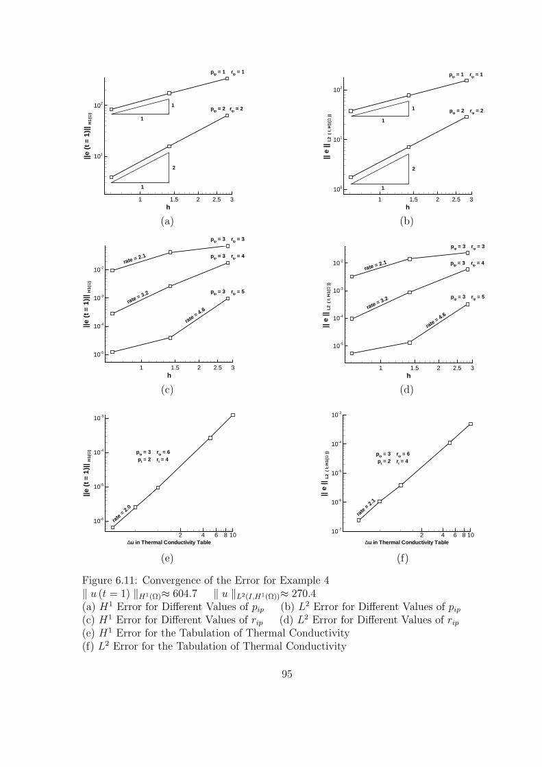
h

||e(t

=1

)|| H

1(Ω

)

1 1.5 2 2.5 3

101

102

pip = 2 rip = 2

pip = 1 rip = 1

1

1

2

1

(a)

h

||e

||L

2(

I;H

1(Ω

))

1 1.5 2 2.5 3

100

101

102

pip = 2 rip = 2

pip = 1 rip = 1

1

1

1

2

(b)

h

||e(t

=1)

||H

1(Ω

)

1 1.5 2 2.5 3

10-5

10-4

10-3

10-2rate = 2.1

rate= 4.6

rate = 3.2 pip = 3 rip = 5

pip = 3 rip = 3

pip = 3 rip = 4

(c)

h

||e

||L

2(

I;H

1(Ω

))

1 1.5 2 2.5 3

10-5

10-4

10-3

10-2

rate = 2.1

rate= 4.6

rate = 3.2 pip = 3 rip = 5

pip = 3 rip = 3

pip = 3 rip = 4

(d)

∆u in Thermal Conductivity Table

||e(t

=1

)|| H

1(Ω

)

2 4 6 8 10

10-6

10-5

10-4

10-3

rate

= 2.0

pip = 3 rip = 6pt = 2 rt = 4

(e)

∆u in Thermal Conductivity Table

||e

||L

2(

I;H

1(Ω

))

2 4 6 8 1010-7

10-6

10-5

10-4

10-3

rate

= 2.1

pip = 3 rip = 6pt = 2 rt = 4

(f)

Figure 6.11: Convergence of the Error for Example 4‖ u (t = 1) ‖H1(Ω)≈ 604.7 ‖ u ‖L2(I,H1(Ω))≈ 270.4(a) H1 Error for Different Values of pip (b) L2 Error for Different Values of pip

(c) H1 Error for Different Values of rip (d) L2 Error for Different Values of rip

(e) H1 Error for the Tabulation of Thermal Conductivity(f) L2 Error for the Tabulation of Thermal Conductivity

95

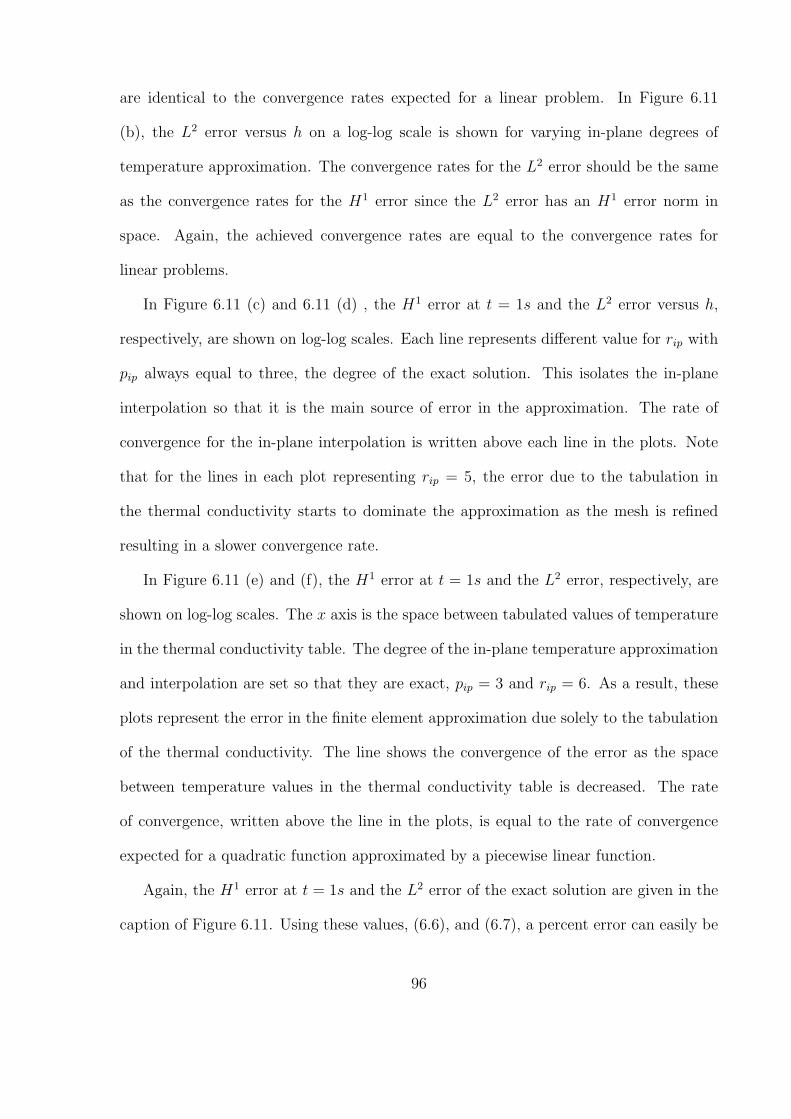
are identical to the convergence rates expected for a linear problem. In Figure 6.11

(b), the L2 error versus h on a log-log scale is shown for varying in-plane degrees of

temperature approximation. The convergence rates for the L2 error should be the same

as the convergence rates for the H1 error since the L2 error has an H1 error norm in

space. Again, the achieved convergence rates are equal to the convergence rates for

linear problems.

In Figure 6.11 (c) and 6.11 (d) , the H1 error at t = 1s and the L2 error versus h,

respectively, are shown on log-log scales. Each line represents different value for rip with

pip always equal to three, the degree of the exact solution. This isolates the in-plane

interpolation so that it is the main source of error in the approximation. The rate of

convergence for the in-plane interpolation is written above each line in the plots. Note

that for the lines in each plot representing rip = 5, the error due to the tabulation in

the thermal conductivity starts to dominate the approximation as the mesh is refined

resulting in a slower convergence rate.

In Figure 6.11 (e) and (f), the H1 error at t = 1s and the L2 error, respectively, are

shown on log-log scales. The x axis is the space between tabulated values of temperature

in the thermal conductivity table. The degree of the in-plane temperature approximation

and interpolation are set so that they are exact, pip = 3 and rip = 6. As a result, these

plots represent the error in the finite element approximation due solely to the tabulation

of the thermal conductivity. The line shows the convergence of the error as the space

between temperature values in the thermal conductivity table is decreased. The rate

of convergence, written above the line in the plots, is equal to the rate of convergence

expected for a quadratic function approximated by a piecewise linear function.

Again, the H1 error at t = 1s and the L2 error of the exact solution are given in the

caption of Figure 6.11. Using these values, (6.6), and (6.7), a percent error can easily be

96

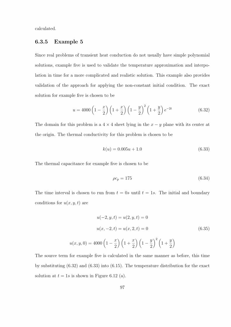
calculated.

6.3.5 Example 5

Since real problems of transient heat conduction do not usually have simple polynomial

solutions, example five is used to validate the temperature approximation and interpo-

lation in time for a more complicated and realistic solution. This example also provides

validation of the approach for applying the non-constant initial condition. The exact

solution for example five is chosen to be

u = 4000(1− x

2

) (1 +

x

2

) (1− y

2

)2 (1 +

y

2

)e−2t (6.32)

The domain for this problem is a 4× 4 sheet lying in the x− y plane with its center at

the origin. The thermal conductivity for this problem is chosen to be

k(u) = 0.005u + 1.0 (6.33)

The thermal capacitance for example five is chosen to be

ρcp = 175 (6.34)

The time interval is chosen to run from t = 0s until t = 1s. The initial and boundary

conditions for u(x, y, t) are

u(−2, y, t) = u(2, y, t) = 0

u(x,−2, t) = u(x, 2, t) = 0 (6.35)

u(x, y, 0) = 4000(1− x

2

) (1 +

x

2

) (1− y

2

)2 (1 +

y

2

)

The source term for example five is calculated in the same manner as before, this time

by substituting (6.32) and (6.33) into (6.15). The temperature distribution for the exact

solution at t = 1s is shown in Figure 6.12 (a).

97

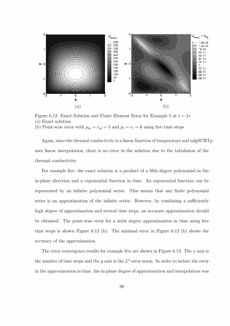
(a) (b)

Figure 6.12: Exact Solution and Finite Element Error for Example 5 at t = 1s(a) Exact solution(b) Point-wise error with pip = rip = 5 and pt = rt = 6 using five time steps

Again, since the thermal conductivity is a linear function of temperature and ndgSCHTp

uses linear interpolation, there is no error in the solution due to the tabulation of the

thermal conductivity.

For example five, the exact solution is a product of a fifth degree polynomial in the

in-plane direction and a exponential function in time. An exponential function can be

represented by an infinite polynomial series. This means that any finite polynomial

series is an approximation of the infinite series. However, by combining a sufficiently

high degree of approximation and several time steps, an accurate approximation should

be obtained. The point-wise error for a sixth degree approximation in time using five

time steps is shown Figure 6.12 (b). The minimal error in Figure 6.12 (b) shows the

accuracy of the approximation.

The error convergence results for example five are shown in Figure 6.13. The x axis is

the number of time steps and the y axis is the L2 error norm. In order to isolate the error

in the approximation in time, the in-plane degree of approximation and interpolation was

98

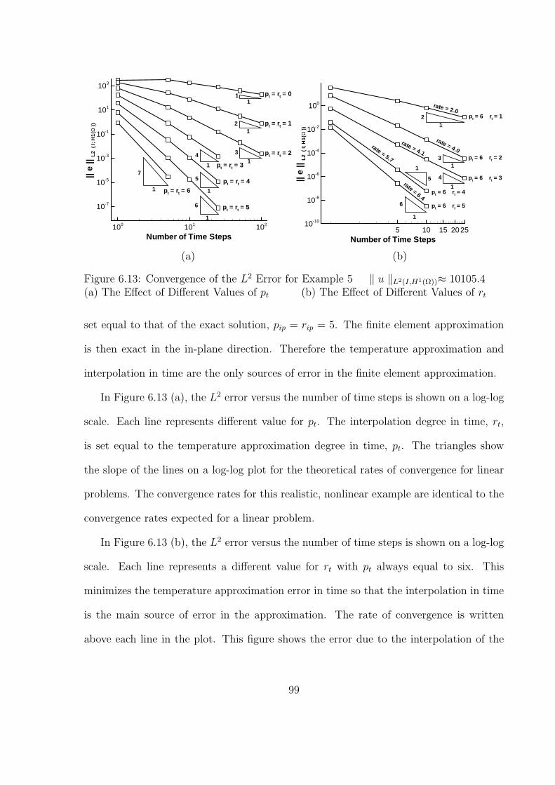
Number of Time Steps

||e

||L

2(

I;H

1(Ω

))

100 101 102

10-7

10-5

10-3

10-1

101

103

pt = rt = 6

1

1

11

1

1

1

1

2

34

5

6

7

pt = rt = 1

pt = rt = 2

pt = rt = 3

pt = rt = 4

pt = rt = 5

pt = rt = 0

(a)

Number of Time Steps

||e

||L

2(

I;H

1(Ω

))

5 10 15 20 2510-10

10-8

10-6

10-4

10-2

100

pt = 6 rt = 1

pt = 6 rt = 4

pt = 6 rt = 2

pt = 6 rt = 3

pt = 6 rt = 5

1

1

1

1

1

2

3

45

6

rate = 6.4

rate = 2.0

rate = 4.0rate = 4.1

rate = 5.7

(b)

Figure 6.13: Convergence of the L2 Error for Example 5 ‖ u ‖L2(I,H1(Ω))≈ 10105.4(a) The Effect of Different Values of pt (b) The Effect of Different Values of rt

set equal to that of the exact solution, pip = rip = 5. The finite element approximation

is then exact in the in-plane direction. Therefore the temperature approximation and

interpolation in time are the only sources of error in the finite element approximation.

In Figure 6.13 (a), the L2 error versus the number of time steps is shown on a log-log

scale. Each line represents different value for pt. The interpolation degree in time, rt,

is set equal to the temperature approximation degree in time, pt. The triangles show

the slope of the lines on a log-log plot for the theoretical rates of convergence for linear

problems. The convergence rates for this realistic, nonlinear example are identical to the

convergence rates expected for a linear problem.

In Figure 6.13 (b), the L2 error versus the number of time steps is shown on a log-log

scale. Each line represents a different value for rt with pt always equal to six. This

minimizes the temperature approximation error in time so that the interpolation in time

is the main source of error in the approximation. The rate of convergence is written

above each line in the plot. This figure shows the error due to the interpolation of the

99

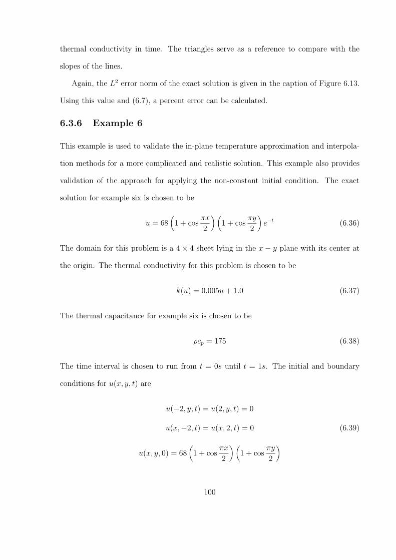
thermal conductivity in time. The triangles serve as a reference to compare with the

slopes of the lines.

Again, the L2 error norm of the exact solution is given in the caption of Figure 6.13.

Using this value and (6.7), a percent error can be calculated.

6.3.6 Example 6

This example is used to validate the in-plane temperature approximation and interpola-

tion methods for a more complicated and realistic solution. This example also provides

validation of the approach for applying the non-constant initial condition. The exact

solution for example six is chosen to be

u = 68(1 + cos

πx

2

) (1 + cos

πy

2

)e−t (6.36)

The domain for this problem is a 4× 4 sheet lying in the x− y plane with its center at

the origin. The thermal conductivity for this problem is chosen to be

k(u) = 0.005u + 1.0 (6.37)

The thermal capacitance for example six is chosen to be

ρcp = 175 (6.38)

The time interval is chosen to run from t = 0s until t = 1s. The initial and boundary

conditions for u(x, y, t) are

u(−2, y, t) = u(2, y, t) = 0

u(x,−2, t) = u(x, 2, t) = 0 (6.39)

u(x, y, 0) = 68(1 + cos

πx

2

) (1 + cos

πy

2

)

100

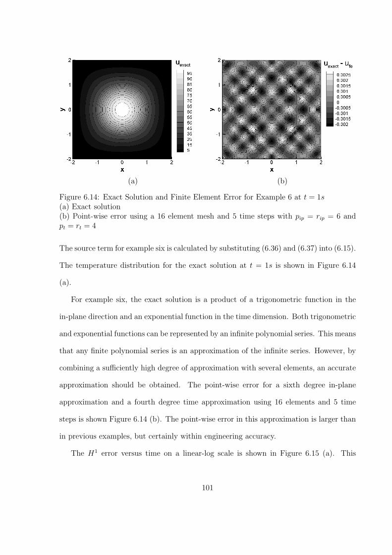
(a) (b)

Figure 6.14: Exact Solution and Finite Element Error for Example 6 at t = 1s(a) Exact solution(b) Point-wise error using a 16 element mesh and 5 time steps with pip = rip = 6 andpt = rt = 4

The source term for example six is calculated by substituting (6.36) and (6.37) into (6.15).

The temperature distribution for the exact solution at t = 1s is shown in Figure 6.14

(a).

For example six, the exact solution is a product of a trigonometric function in the

in-plane direction and an exponential function in the time dimension. Both trigonometric

and exponential functions can be represented by an infinite polynomial series. This means

that any finite polynomial series is an approximation of the infinite series. However, by

combining a sufficiently high degree of approximation with several elements, an accurate

approximation should be obtained. The point-wise error for a sixth degree in-plane

approximation and a fourth degree time approximation using 16 elements and 5 time

steps is shown Figure 6.14 (b). The point-wise error in this approximation is larger than

in previous examples, but certainly within engineering accuracy.

The H1 error versus time on a linear-log scale is shown in Figure 6.15 (a). This

101

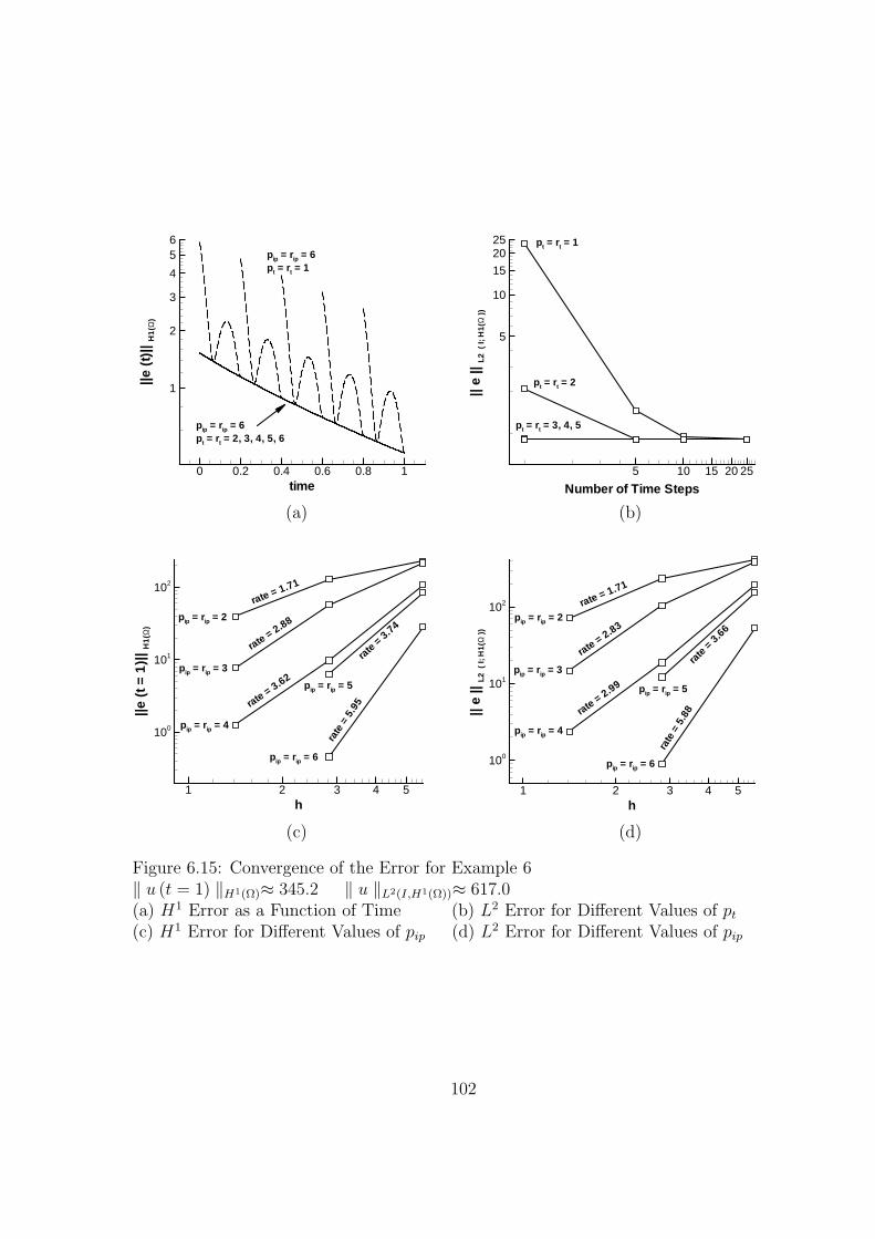
time

||e(t

)|| H

1(Ω

)

0 0.2 0.4 0.6 0.8 1

1

2

3

4

56

pip = rip = 6pt = rt = 2, 3, 4, 5, 6

pip = rip = 6pt = rt = 1

(a)

Number of Time Steps||

e||

L2

(I;

H1(

Ω))

5 10 15 20 25

5

10

15

2025

pt = rt = 3, 4, 5

pt = rt = 1

pt = rt = 2

(b)

h

||e(t

=1

)|| H

1(Ω

)

1 2 3 4 5

100

101

102

rate= 2.88

rate

=5.

95rate= 3.62

rate

= 3.74

rate = 1.71

pip = rip = 6

pip = rip = 2

pip = rip = 3

pip = rip = 4

pip = rip = 5

(c)

h

||e

||L

2(

I;H

1(Ω

))

1 2 3 4 5

100

101

102

pip = rip = 6

pip = rip = 2

pip = rip = 3

pip = rip = 4

pip = rip = 5

rate

=5.

88

rate = 1.71

rate= 2.83

rate= 2.99

rate

=3.6

6

(d)

Figure 6.15: Convergence of the Error for Example 6‖ u (t = 1) ‖H1(Ω)≈ 345.2 ‖ u ‖L2(I,H1(Ω))≈ 617.0(a) H1 Error as a Function of Time (b) L2 Error for Different Values of pt

(c) H1 Error for Different Values of pip (d) L2 Error for Different Values of pip

102

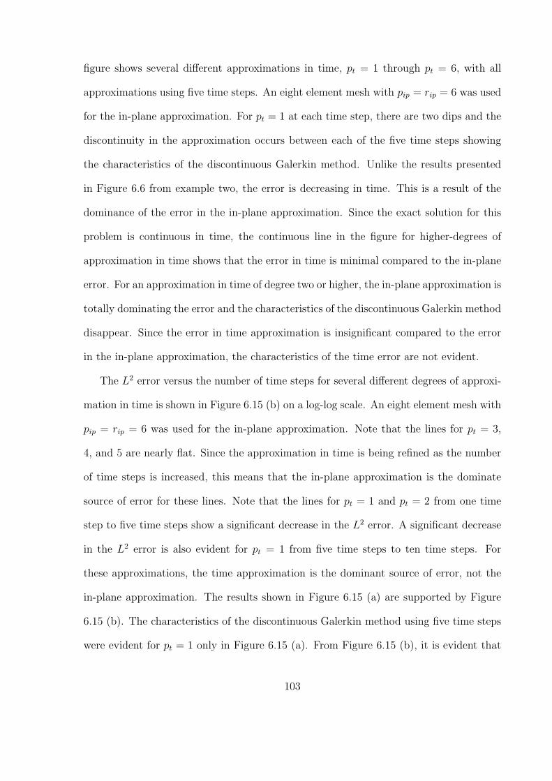
figure shows several different approximations in time, pt = 1 through pt = 6, with all

approximations using five time steps. An eight element mesh with pip = rip = 6 was used

for the in-plane approximation. For pt = 1 at each time step, there are two dips and the

discontinuity in the approximation occurs between each of the five time steps showing

the characteristics of the discontinuous Galerkin method. Unlike the results presented

in Figure 6.6 from example two, the error is decreasing in time. This is a result of the

dominance of the error in the in-plane approximation. Since the exact solution for this

problem is continuous in time, the continuous line in the figure for higher-degrees of

approximation in time shows that the error in time is minimal compared to the in-plane

error. For an approximation in time of degree two or higher, the in-plane approximation is

totally dominating the error and the characteristics of the discontinuous Galerkin method

disappear. Since the error in time approximation is insignificant compared to the error

in the in-plane approximation, the characteristics of the time error are not evident.

The L2 error versus the number of time steps for several different degrees of approxi-

mation in time is shown in Figure 6.15 (b) on a log-log scale. An eight element mesh with

pip = rip = 6 was used for the in-plane approximation. Note that the lines for pt = 3,

4, and 5 are nearly flat. Since the approximation in time is being refined as the number

of time steps is increased, this means that the in-plane approximation is the dominate

source of error for these lines. Note that the lines for pt = 1 and pt = 2 from one time

step to five time steps show a significant decrease in the L2 error. A significant decrease

in the L2 error is also evident for pt = 1 from five time steps to ten time steps. For

these approximations, the time approximation is the dominant source of error, not the

in-plane approximation. The results shown in Figure 6.15 (a) are supported by Figure

6.15 (b). The characteristics of the discontinuous Galerkin method using five time steps

were evident for pt = 1 only in Figure 6.15 (a). From Figure 6.15 (b), it is evident that

103

for approximations in time higher than degree one using five time steps, the in-plane

approximation is dominating the error.

In Figure 6.15 (c), the H1 error versus h at t = 1s is shown on a log-log scale. Each

line represents different value for pip = rip. For this plot, pt = rt = 6 and five time

steps were used for the approximation in time. The convergence rates for the in-plane

approximation are all less than the convergence rates expected for a linear problem.

These reduced convergence rates are a result of the error in the approximation in time.

Although the in-plane approximation is clearly dominating the error as shown in Figure

6.15 (b), the approximation in time is contributing to the error and slowing the rate of

convergence for the in-plane approximations.

The slowing of the in-plane convergence rates due to the error in the approximation

in time is supported by Figure 6.15 (d). In this figure, the L2 error versus the mesh size

is shown on a log-log scale. The same degrees of approximation in time and space along

with the same mesh and number of time steps from Figure 6.15 (c) were used in this

figure. Note the decreased rates of convergence in Figure 6.15 (d) compared to Figure

6.15 (c). These decreased rates are a result of the integration over the error in time for

the L2 error as compared to the H1 error which is just evaluated at a point in time.

From the sample problems presented in this research, the linear convergence rates are

valid for nonlinear problems only when a single source of error in the approximation can

be isolated. As shown in the first five examples, when the in-plane or time approximation

is isolated, the linear convergence rates apply to these nonlinear problems. In example

six, the error convergence rates are less than those expected for linear problems because

there is error in both the in-plane and time approximations.

104

Chapter 7

Concluding Remarks

Finite element methods are used to accurately predict the thermal response of a structure

during reentry and hypersonic travel through the atmosphere. Many commercial finite

element codes currently rely on separate meshes for structural and thermal analyses.

These codes also rely upon mesh regeneration to improve the solution using h-version

or traditional p-version elements. The commercial codes use finite element methods in

space and finite difference schemes in time. Finite difference schemes in time require

small time steps for accuracy and stability. The conduction heat transfer problem is

nonlinear due to the variation in the thermal conductivity with temperature. Current

finite element methods for nonlinear problems utilize one of two approaches. Either the

thermal conductivity is assumed to be constant over each element or the finite element

integrals containing the thermal conductivity are integrated using Gaussian quadrature.

A hierarchical p-version space-time finite element method with a structurally com-

patible mesh for nonlinear, transient problems was developed and tested in this research.

Hierarchical, p-version finite elements allowed higher degrees of approximation on each

element and eliminated the need for new meshes as the degree of approximation is in-

creased. Three different sets of hierarchical basis functions, one each for the in-plane,

time, and through-thickness dimensions, were used to approximate the temperature dis-

tribution over an element. The hierarchical modelling also allowed a three-dimensional

105

domain to be collapsed onto a two-dimensional, structurally-compatible mesh. The p-

version discontinuous Galerkin method allows higher degrees of approximation in time

and provides stability regardless of the size of the time step. Higher-degree interpolants

were used over each element to accurately capture the variation in the thermal conduc-

tivity. The interpolants utilized three different sets of interpolation functions, one each

for the in-plane, time, and through-thickness dimensions, to account for the temperature-

dependent thermal conductivity. The finite element method presented in this research

eliminates many of the limitations of commercial finite element codes. The finite element

formulation was tested in a FORTRAN code called ndgSCHTp. To increase the efficiency

of ndgSCHTp, master matrices were utilized. The FORTRAN code was validated for

nonlinear problems constructed to have exact solutions so the error between the finite

element approximation and the exact solution could be quantified.

The finite element method presented in this research provided accurate solutions to

nonlinear, transient problems of conduction heat transfer. For simple polynomial exact

solutions in space and time, ndgSCHTp reproduces the exact solutions to within machine

precision. Accurate solutions were also obtained for non-polynomial exact solutions. The

error due to the tabulation of the thermal conductivity was explored and its effect on

the finite element approximation was shown. The H1 and L2 error convergence rates

for these nonlinear problems were shown to agree with the theoretical convergence rates

for linear problems when a single source of error could be isolated. The finite element

method developed was shown to be very accurate for transient, nonlinear problems of

conduction heat transfer.

There are several areas of future research that should be explored relating to this work.

Problems with complicated domains should be explored. These sample problems would

show the robustness of the method presented here and expose any possible problems. The

106

finite element formulation presented in this work has been expanded to include nonlinear

specific heat as a function of temperature, cp(u), using the same interpolation method

used for the thermal conductivity. This formulation should be implemented and tested

using a computer code. Layered structures consisting of several different materials are

commonly used in thermal protection systems. The current finite element formulation

should be modified to account for layered structures. The method presented by Lang [8]

for layered structures would be difficult to modify for temperature-dependent thermal

conductivity, so a new method to handle layered materials should be developed. The

finite element formulation should also be extended to include materials with anisotropic

conductivity.

107

References

[1] The MacNeal Schwendler Corporation, NASTRAN User’s Manual, 1995.

[2] Abaqus Inc., ABAQUS / Standard User’s Manual.

[3] Surana, K.S. and Orth, N.J., “Completely Hierarchical p-Version Axisymmetric

Shell Element for Nonlinear Heat Conduction in Laminated Composites,” Com-

puters and Structures, Vol.46, No.5, 1993, pp. 777-789.

[4] Szabo, B. and Babuska, I., Finite Element Analysis, John Wiley & Sons Inc., New

York, 1981.

[5] Tamma, K. and Saw, K.,“Hierarchical p-Version Finite Elements and Adaptive a

Posteriori Computational Formulations for Two-Dimensional Thermal Analysis,”

AIAA Paper 89-0518, 1989.

[6] Gould, D., “Hierarchical p-Version Finite Elements for Radiation Heat Transfer,”

Ph.D. Dissertation, University of Virginia, 1999.

[7] Tomey, J. P., “p-Version Discontinuous Galerkin Method for Heat Transfer in Built-

up Structures,” M.S. Thesis, The George Washington University, 2001.

[8] Lang, C. G., “Finite Element A Posteriori Error Estimation for Heat Conduction,”

NASA CR-2002-211958, November 2002.

108

[9] Walker, D. T., “Nonlinear Conduction Heat Transfer Using a Hierarchical Finite

Element Method,” M.S. Thesis, The George Washington University, 2003.

[10] Schotzau, D., Scwab, C., “An hp A-Priori Error Analysis of the DG Time-Stepping

Method for Initial Value Problems,” IMA Resarch Report 1652, University of Min-

nesota, 1999.

[11] Schotzau, D., Scwab, C., “Time Discretization of Parabolic Problems by the hp-

Version of the Discontinuous Galerkin Finite Element Method,” SIAM Journal of

Numerical Analysis, Vol. 38, No. 3, 2000, pp. 837-875.

[12] Eriksson, K., Johnson, C., Larsson, S., “Adaptive Finite Elements for Parabolic

Problems VI: Analytic Semigroups,” SIAM Journal of Numerical Analysis, Vol. 35,

No. 4, 1998, pp. 1315-1325.

[13] Reddy, J. N., An Introduction to the Finite Element Method, Second Edition,

McGraw-Hill, Boston, 1993.

[14] Boas, Mary L., Mathematical Methods in the Physical Sciences, Second Edition,

John Wiley & Sons, New York, 1983.

[15] Hughes, Thomas J.R., The Finite Element Method: Linear Static and Dynamic

Finite Element Analysis, Prentice-Hall, Englewood Cliffs, New Jersey, 1987.

[16] Schotzau, D. and Schwab, C., “Time Discretization of Parabolic Problems by the

HP-Version of the Discontinuous Galerkin Finite Element Method,” SIAM Journal

on Numerical Analysis, Vol.38, No.3, 2000, pp. 837-875.

[17] Chapra, S. C. and Canale, R. P., Numerical Methods for Engineers, WCB McGraw-

Hill, Boston, 1998.

109

[18] Myint-U, T., Debnath, L., Partial Differential Equations for Scientists and Engi-

neers, Third Edition, P T R Prentice Hall, Englewood Cliffs, New Jersey, 1987.

[19] Zienkiewicz, O. C., Morgan, K., Finite Elements and Approximation, John Wiley &

Sons, New York, 1983.

[20] Mish, K., “Two-Dimensional Finite Elements,” U.C.Davis Course Notes ECI212A,

http://cee.engr.ucdavis.edu/Faculty/mish/212A/2dfems.pdf 1

[21] Young, D. M., Gregory, R. T., A Survey of Numerical Mathematics In Two Volumes,

Dover Publications, Inc., New York, 1972.

[22] Rivlin, T. J., Chebyshev Polynomials: From Approximation Theory to Algebra and

Number Theory, John Wiley & Sons, New York, 1990.

[23] Taylor, M. A., Wingate, B. A. and Vincent, R. E., “An Algorithm for computing

Fekete Points In The Triangle,” SIAM Journal, Vol. 38 No. 5, pp 1707-1720, 2000.

[24] Bey, K. S., “The SCHT Code, A User and Programmer’s Manual,” Metals and

Thermal Structures Branch internal document, NASA Langley Research Center,

2002.

[25] Dunavant, D. A., “High Degree Efficient Symmetrical Gaussian Quadrature Rules

for the Triangle,” International Journal for Numerical Methods in Engineering, Vol.

21, 1989, pp. 1129-1148.

[26] Werder, T., Gerdes, K., Schotzau, D., Schwab, C., “hp Discontinuous Galerkin Time

Stepping for Parabolic Problems,” Research Report No. 2000-01 April 2000, Seminar

for Applied Mathematics, ETH Zurich, 2000.

110

[27] Becker, E., Carey, G., Oden, J., Finite Elements: An Introduction, Volume I,

Prentice-Hall Inc., Englewood Cliffs, New Jersey, 1981.

1 Contact the author for copies of World Wide Web references: jcsand@copper.net,

jeromecsanders@yahoo.com

111