nonlinear random vibration using updated tail equivalent ... · nonlinear random vibration using...

ORIGINAL RESEARCH

Nonlinear random vibration using updated tail equivalentlinearization method

Reza Raoufi • Mohsen Ghafory-Ashtiany

Received: 25 November 2013 / Accepted: 21 December 2013 / Published online: 5 March 2014

� The Author(s) 2014. This article is published with open access at Springerlink.com

Abstract Tail equivalent linearization method is based on

first order reliability method, which obtains an equivalent

linear system for the considered nonlinear problem with equal

tail probability related to a specified threshold and time. This

method has been applied only to nonlinear non-degrading

single- and multi-degrees of freedom shear beam two-

dimensional models and three-dimensional one-story rigid

diaphragm supported by frames with in-plane uni-axial stiff-

ness which is subjected to independent random excitation

along the structural axes. To use TELM for more practical

problems it is required to extend this method to cover more

realistic material and excitation characteristics. In this paper,

some of these developments have been presented. Application

of TELM for bi-directional excitation with bi-axial material

subjected to different incidence angles of excitation and using

TELM for degrading material which has been presented in the

previous works of the authors have been reviewed briefly. In

addition a new method for defining rotational dependent

component of earthquake excitation in terms of independent

translational components in the standard normal random

variable space is proposed, and TELM has been used for this

kind of excitation. Three examples related to these extensions

have been presented; the comparison of the TELM results

with Mote-Carlo simulation results shows good agreement.

Keywords Nonlinear random vibration � Reliability �Linearization � Rotational component

Introduction

Most structures under extreme dynamic loads resulting

from natural hazards with low probability exhibit nonlinear

behavior. Accurate prediction of variations of such loads is

impossible and therefore usually these loads are modeled

as random processes. Thus nonlinear random vibration

methods are the best methods in the analysis of the struc-

tures under sever loads associated with natural hazards.

Random vibration for linear structures uses the superposi-

tion principle. However, this advantage is not applicable

for nonlinear systems, but there are ways to transform a

nonlinear system to an equivalent linear system that can

benefit from this privilege. In the conventional method i.e.

equivalent linearization method (ELM) which is widely

used because of its simplicity and applicability to different

systems the equivalent system is selected by minimizing

the mean-square error between the responses of the non-

linear and the linear systems based on the assumption of

Gaussian response for the nonlinear system. Since the

Gaussian assumption is not valid for high nonlinear sys-

tems, although the accuracy of the method is good in

estimating the mean-square response, the probability dis-

tribution can be far from correct, particularly in the tail

region. Thus estimates of response statistics such as

crossing rates and first-passage probability, issues of which

are of particular interest in reliability analysis, can be

grossly inaccurate at high thresholds.

To overcome the shortcomings of the conventional ELM,

Fujimura and Der Kiureghian (2007) presented tail equiva-

lent linearization method (TELM) which uses the advantages

of first order reliability method (FORM). In this method

stochastic excitation is discretized and represented in terms

of a finite set of standard normal random variables. Based on

this representation of excitation, the limit state surface for

R. Raoufi (&) � M. Ghafory-Ashtiany

Department of Civil Engineering, Science and Research Branch,

Islamic Azad University, Tehran, Iran

e-mail: [email protected]

123

Int J Adv Struct Eng (2014) 6:45

DOI 10.1007/s40091-014-0045-6

desired response at a specified time instant can be stated in

terms of these variables. In TELM the nonlinear limit state of

the specified response threshold and time is linearized at the

nearest point to the origin. Based on the rotational symmetry

and exponential decaying of the standard normal probability

density function, this point which is called design point in

FORM has the maximum likelihood among all points on the

limit state surface and has the most contribution in the

probability of failure. Tail equivalent linear system (TELS)

is defined based on the linearized limit state surface, because

its tail probability is equal to the tail probability of the non-

linear system. This definition is accomplished by unit

impulse response functions (IRFs) for nonlinear system for

each direction of excitation. These IRFs can be used to obtain

the statistical properties of the nonlinear system by linear

random vibration methods.

This method could predict probability density function

(PDF), cumulative distribution function (CDF), crossing

rate and first-passage probability with good accuracy.

Furthermore, since the linear system with equivalent tail is

dependent on the specified threshold the method is capable

to predict the non-Gaussian distribution of the nonlinear

response. In addition, due to the invariance of TELS on the

scale of the excitation estimates for a sequence of scaled

excitations (fragility analysis) can be performed with a

single determination of the TELS (Fujimura and Der

Kiureghian 2007; Der Kiureghian and Fujimura 2009).

TELM has been applied to single- and multi-degrees of

freedom 2D shear beam frames and stick-like models by

Fujimura and Der Kiureghian (2007) and Der Kiureghian

and Fujimura (2009); and to 3D structures with rigid dia-

phragm subjected to independent bi-directional excitation

along the structural axes for uni-axial Bouc–Wen material

by Broccardo and Der Kiureghian (2012).

To apply the TELM to more realistic problems, fol-

lowing points need to be considered:

• Bi-axial material behavior for the bi-directional

excitation;

• Materials show degradation behavior. This point has

not been considered in the previous studies;

• The independent components of excitation are not

along the major axes of structure;

• The rotational component of excitation (especially for

earthquake excitation). Considering that it is not possible

to define this component as a statistically independent

component from horizontal components, a new method

for simulating this component in terms of translational

components of earthquake has been presented.

In a new study, the authors extended TELM to bi-axial

Bouc–Wen material subjected to bi-directional excitation

along or not along the structural axes in Raoofi and Ghaf-

ory-Ashtiany (2013a) and Ghafory-Ashtiany and Raoofi

(2013). Furthermore, the authors have developed modified

TELM method for considering degradation of materials for

un-axial Bouc–Wen model in 2D and 3D arrangements

Raoofi and Ghafory-Ashtiany (2013b). In this paper, in

addition to reviewing these findings, a new method for

defining the rotational component of earthquake excitation

has been presented, and TELM method has been applied

with considering this component of excitation.

A brief review on TELM

The first step in the application of FORM or TELM is

temporal discretizing of the excitation in terms of standard

normal random variables. It is assumed that the compo-

nents of the multi-directional excitation are statistically

independent and can be stated as follows (Rezaeian and

Der Kirureghian 2011):

fj tð Þ ¼Xn

i¼1

uið Þ

j sið Þ

j tð Þ ¼ sj tð Þuj j ¼ 1; . . .;m ð1Þ

is the component of the base excitation in the jth direction

at discrete time point t ¼ t0; t1; . . .; ti; ; . . .; tn where

ti ¼ i � Dt. In this representation of excitation uj ¼ uð1Þj ;

n

uð2Þj ; . . .; u

ðnÞj gT

and sj tð Þ ¼ sð1Þj tð Þ; s

ð2Þj tð Þ; . . .; s

ðnÞj tð Þ

n oT

are

vectors of standard normal random variables and

deterministic basis functions in the j ¼ 1; . . .;m

directions, respectively. Thus u ¼ u1; u2; � � � ; um½ �Trepresents the uncertainty of the excitation and, therefore,

is a vector which represents the uncertainty of the problem

with m 9 n elements. In this paper sj(t) vectors are

calculated based on the presented method in Fujimura

and Der Kiureghian (2007) and Rezaeian and Der

Kirureghian (2011). For a linear system using

superposition role, the desired response v tð Þ which is

affected by the multi-component base excitation can be

written as follows:

v tð Þ ¼Xm

j¼1

Z t

0

fj sð Þhj t � sð Þds ð2Þ

where hj tð Þ is the IRF in the jth direction. By substituting

Eq. 1 into 2:

v tð Þ ¼Xm

j¼1

Z t

0

Xn

i¼1

uið Þ

j sið Þ

j sð Þhj t � sð Þds

¼Xm

j¼1

Xn

i¼1

uið Þ

j aið Þ

j tð Þ ¼Xm

j¼1

aj tð Þuja

ð3Þ

where aið Þ

j tð Þ ¼R t

0s

ið Þj sð Þhj t � sð Þds and aj tð Þ ¼

a1ð Þ

j tð Þ; a2ð Þ

j tð Þ; . . .; anj tð Þ

h i. With the definition a tð Þ ¼

45 of 12 Int J Adv Struct Eng (2014) 6:45

123

a1 tð Þ; a2 tð Þ; . . .; am tð Þ½ �, the above equation can be written

as v tð Þ ¼ a tð Þ � u and this means that for linear systems the

response can be stated as the product of two vectors which

one of them is deterministic time variant and the other is

random time invariant, if the excitation is stated as the

product of two vectors like Eq. 1.

The limit state surface for a linear structure with consid-

ering the response threshold X at time point tn can be written

as G uð Þ ¼ X � v tnð Þ ¼ X � a tnð Þu which is a hyper-plane in

the m 9 n dimensional space of normal random variables.

For nonlinear systems Eq. 2 and 3 are not valid but the

nonlinear limit state surface G(u) = X-v(tn) can be

approximated by a hyper-plane at the nearest point to the

origin u� of the normal random variable space in TELM.

For finding u� which is called design point in reliability, a

constrained optimization problem should be solved in a

standard normal space with dimensions equal to the ele-

ments of uvector. Design point u� is a point on the limit

state surface, G u�ð Þ ¼ 0, with minimum distance from the

origin. For obtaining u� the response of the structure and its

gradient should be calculated and used in a proper opti-

mization framework.

After solving the optimization problem, the non-

Gaussian response is replaced by a Gaussian one which is

defined by the based function vector a tnð Þ ¼ruv u; tnð Þju¼u� X;tnð Þ and the probability of failure could be

expressed by U �b X; tnð Þð Þ, where b is called reliability

index and is equal to Euclidean norm of u�, where U(.) is

the standard normal CDF. Based on the geometric prop-

erties, a(tn) vector can be obtained from the following

equation (Fujimura and Der Kiureghian 2007):

a tnð Þ ¼ X

k u� X; tnð Þ ku� X; tnð Þ

k u� X; tnð Þ k ð4Þ

The obtained vector from the above equation separated

to m vectors a1 to am each with n elements. Then the IRFs

of TELS can be obtained from the following equations for

j ¼ 1; . . .;m.

Xn

k¼1

hj tn � tkð Þs ið Þj tkð ÞDt ffi a

ið Þj tnð Þ; i ¼ 1; . . .; n ð5Þ

Each of the above relations represent a set of n equations

which can be solved for the values of the IRFs at time

points. The obtained IRFs indicate TELS for the specified

threshold X and time point tn and define a linear system in

the space of u variables which has an identical design point

with the nonlinear system.

By obtaining the IRFs or frequency response functions

(FRFs) (by the Fourier transform of IRFs) of equivalent

linear system, linear random vibration methods can be used

to determine the considered statistical responses for the

nonlinear system with first order approximation.

Application of the TELM for bi-axial materials

and bi-directional excitation with incident angle h

Finding the design point is the most computational part in

applying TELM. This point is the solution of a constrained

optimization problem, which requires calculating the

response and its gradient with respect to random variables

for several times. Due to the large number of standard

normal random variables in stochastic dynamic, this gra-

dient computation should be done by direct differentiation

method (DDM) algorithm. Thus to apply TELM to dif-

ferent material models DDM algorithm for those models

should be developed. In a recent work the authors have

developed bi-axial Bouc–Wen DDM computation for use

in TELM (Raoofi and Ghafory-Ashtiany 2013a). TELS and

the statistics of the response for a 3D structure with rigid

diaphragm supported by four columns with bi-axial Bouc–

Wen material subjected to independent white noise and

modulated filtered white noise along the structural axes

have been obtained, and showed good agreement in com-

parison with simulation results. But in general the statis-

tically independent components of excitation are not along

the structural axes (Penzien and Watabe 1975; Singh and

Ghafory-Ashtiany 1984). Thus the authors present TELM

for considering incident angle of independent components

of excitation in Ghafory-Ashtiany and Raoofi (2013). In the

latter case the obtained IRFs are along the principal

directions of excitation (these are orthogonal directions

where the components of excitation can be stated as

uncorrelated and statistically independent components

along them) not along structural axes. In other words, if p

and q are perpendicular directions which relate to the

principal axes of excitation, subscript j in the Eqs. 1 and 6

is j = p, q and the uncertainty vector of the problem is

u ¼ up; uq

� �T. The following example shows the capabil-

ities of the method.

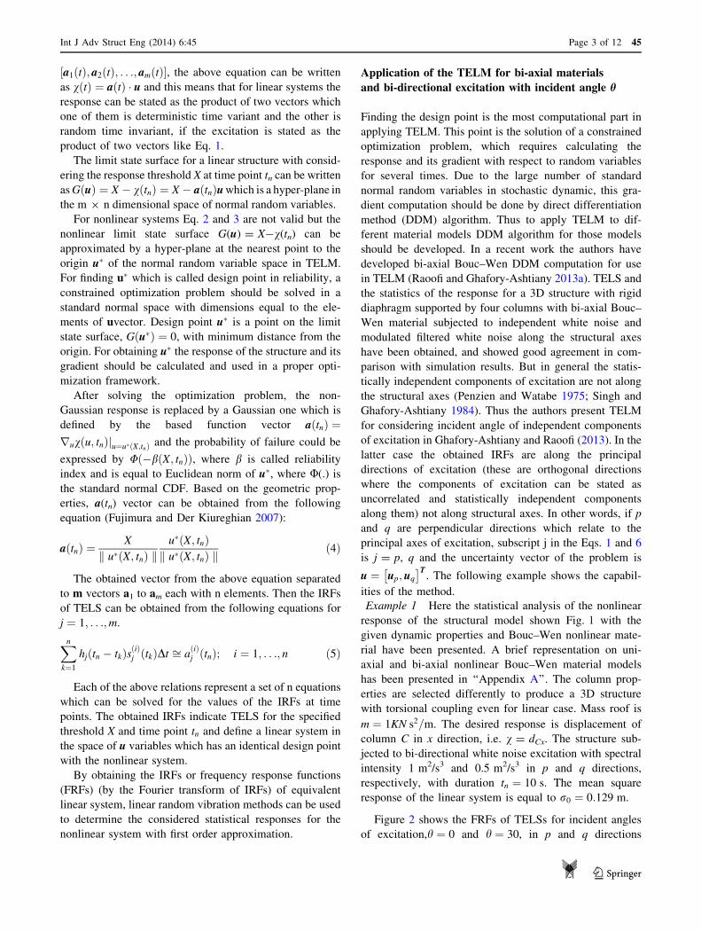
Example 1 Here the statistical analysis of the nonlinear

response of the structural model shown Fig. 1 with the

given dynamic properties and Bouc–Wen nonlinear mate-

rial have been presented. A brief representation on uni-

axial and bi-axial nonlinear Bouc–Wen material models

has been presented in ‘‘Appendix A’’. The column prop-

erties are selected differently to produce a 3D structure

with torsional coupling even for linear case. Mass roof is

m ¼ 1KN s2=m. The desired response is displacement of

column C in x direction, i.e. v = dCx. The structure sub-

jected to bi-directional white noise excitation with spectral

intensity 1 m2/s3 and 0.5 m2/s3 in p and q directions,

respectively, with duration tn ¼ 10 s. The mean square

response of the linear system is equal to r0 ¼ 0:129 m.

Figure 2 shows the FRFs of TELSs for incident angles

of excitation,h ¼ 0 and h ¼ 30, in p and q directions

Int J Adv Struct Eng (2014) 6:45 of 12 45

123

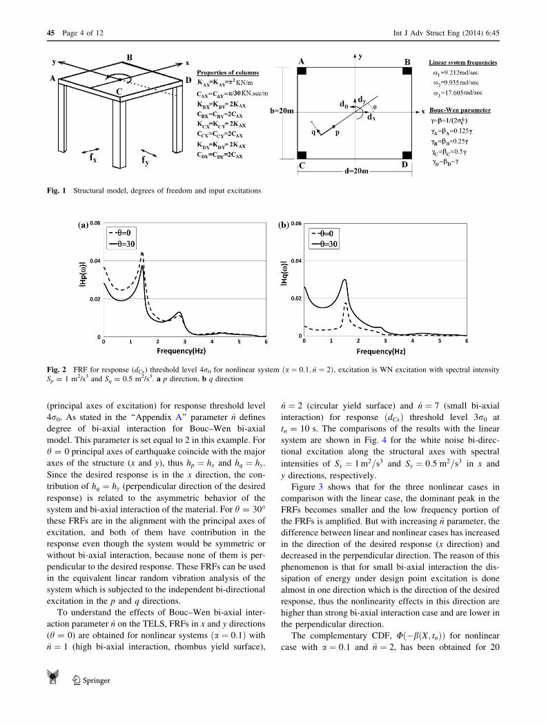
(principal axes of excitation) for response threshold level

4r0. As stated in the ‘‘Appendix A’’ parameter n̂ defines

degree of bi-axial interaction for Bouc–Wen bi-axial

model. This parameter is set equal to 2 in this example. For

h = 0 principal axes of earthquake coincide with the major

axes of the structure (x and y), thus hp ¼ hx and hq ¼ hy.

Since the desired response is in the x direction, the con-

tribution of hq ¼ hy (perpendicular direction of the desired

response) is related to the asymmetric behavior of the

system and bi-axial interaction of the material. For h = 30�these FRFs are in the alignment with the principal axes of

excitation, and both of them have contribution in the

response even though the system would be symmetric or

without bi-axial interaction, because none of them is per-

pendicular to the desired response. These FRFs can be used

in the equivalent linear random vibration analysis of the

system which is subjected to the independent bi-directional

excitation in the p and q directions.

To understand the effects of Bouc–Wen bi-axial inter-

action parameter n̂ on the TELS, FRFs in x and y directions

(h = 0) are obtained for nonlinear systems ða ¼ 0:1Þ with

n̂ ¼ 1 (high bi-axial interaction, rhombus yield surface),

n̂ ¼ 2 (circular yield surface) and n̂ ¼ 7 (small bi-axial

interaction) for response dCxð Þ threshold level 3r0 at

tn = 10 s. The comparisons of the results with the linear

system are shown in Fig. 4 for the white noise bi-direc-

tional excitation along the structural axes with spectral

intensities of Sx ¼ 1 m2=s3 and Sy ¼ 0:5 m2=s3 in x and

y directions, respectively.

Figure 3 shows that for the three nonlinear cases in

comparison with the linear case, the dominant peak in the

FRFs becomes smaller and the low frequency portion of

the FRFs is amplified. But with increasing n̂ parameter, the

difference between linear and nonlinear cases has increased

in the direction of the desired response (x direction) and

decreased in the perpendicular direction. The reason of this

phenomenon is that for small bi-axial interaction the dis-

sipation of energy under design point excitation is done

almost in one direction which is the direction of the desired

response, thus the nonlinearity effects in this direction are

higher than strong bi-axial interaction case and are lower in

the perpendicular direction.

The complementary CDF, U �b X; tnð Þð Þ for nonlinear

case with a ¼ 0:1 and n̂ ¼ 2, has been obtained for 20

Fig. 1 Structural model, degrees of freedom and input excitations

Fig. 2 FRF for response (dCx) threshold level 4r0 for nonlinear system a ¼ 0:1; n̂ ¼ 2ð Þ, excitation is WN excitation with spectral intensity

Sp = 1 m2/s3 and Sq = 0.5 m2/s3. a p direction, b q direction


123

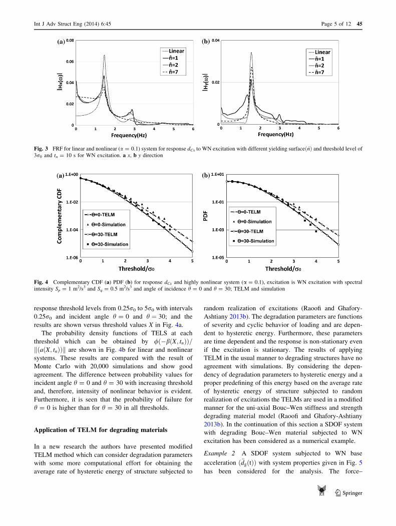
response threshold levels from 0.25r0 to 5r0 with intervals

0.25r0 and incident angle h = 0 and h ¼ 30; and the

results are shown versus threshold values X in Fig. 4a.

The probability density functions of TELS at each

threshold which can be obtained by / �b X; tnð Þð Þ=a X; tnð Þð Þk k are shown in Fig. 4b for linear and nonlinear

systems. These results are compared with the result of

Monte Carlo with 20,000 simulations and show good

agreement. The difference between probability values for

incident angle h = 0 and h = 30 with increasing threshold

and, therefore, intensity of nonlinear behavior is evident.

Furthermore, it is seen that the probability of failure for

h = 0 is higher than for h = 30 in all thresholds.

Application of TELM for degrading materials

In a new research the authors have presented modified

TELM method which can consider degradation parameters

with some more computational effort for obtaining the

average rate of hysteretic energy of structure subjected to

random realization of excitations (Raoofi and Ghafory-

Ashtiany 2013b). The degradation parameters are functions

of severity and cyclic behavior of loading and are depen-

dent to hysteretic energy. Furthermore, these parameters

are time dependent and the response is non-stationary even

if the excitation is stationary. The results of applying

TELM in the usual manner to degrading structures have no

agreement with simulations. By considering the depen-

dency of degradation parameters to hysteretic energy and a

proper predefining of this energy based on the average rate

of hysteretic energy of structure subjected to random

realization of excitations the TELMs are used in a modified

manner for the uni-axial Bouc–Wen stiffness and strength

degrading material model (Raoofi and Ghafory-Ashtiany

2013b). In the continuation of this section a SDOF system

with degrading Bouc–Wen material subjected to WN

excitation has been considered as a numerical example.

Example 2 A SDOF system subjected to WN base

acceleration ð€dg tð ÞÞ with system properties given in Fig. 5

has been considered for the analysis. The force–

Fig. 3 FRF for linear and nonlinear (a = 0.1) system for response dCx to WN excitation with different yielding surface n̂ð Þ and threshold level of

3r0 and tn = 10 s for WN excitation. a x, b y direction

Fig. 4 Complementary CDF (a) PDF (b) for response dCx and highly nonlinear system (a = 0.1), excitation is WN excitation with spectral

intensity Sp = 1 m2/s3 and Sq = 0.5 m2/s3 and angle of incidence h = 0 and h = 30; TELM and simulation


123

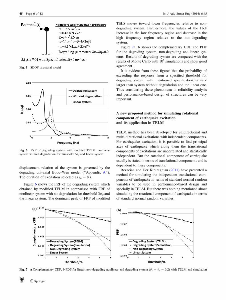
displacement relation of the system is governed by the

degrading uni-axial Bouc–Wen model (‘‘Appendix A’’).

The duration of excitation selected as tn ¼ 8 s.

Figure 6 shows the FRF of the degrading system which

obtained by modified TELM in comparison with FRF of

nonlinear system with no-degradation for threshold 3r0 and

the linear system. The dominant peak of FRF of modified

TELS moves toward lower frequencies relative to non-

degrading system. Furthermore, the values of the FRF

increase in the low frequency region and decrease in the

high frequency region relative to the non-degrading

system.

Figure 7a, b shows the complementary CDF and PDF

for the degrading system, non-degrading and linear sys-

tems. Results of degrading system are compared with the

results of Monte Carlo with 105 simulations and show good

agreement.

It is evident from these figures that the probability of

exceeding the response from a specified threshold for

degrading system with mentioned specification is very

larger than system without degradation and the linear one.

Thus considering these phenomena in reliability analysis

and performance-based design of structures can be very

important.

A new proposed method for simulating rotational

component of earthquake excitation

and its application in TELM

TELM method has been developed for unidirectional and

multi-directional excitations with independent components.

For earthquake excitation, it is possible to find principal

axes of earthquake which along them the translational

components of excitations are uncorrelated and statistically

independent. But the rotational component of earthquake

usually is stated in terms of translational components and is

dependent to these components.

Rezaeian and Der Kirureghian (2011) have presented a

method for simulating the independent translational com-

ponents of earthquake in terms of standard normal random

variables to be used in performance-based design and

specially in TELM. But there was nothing mentioned about

simulating the rotational component of earthquake in terms

of standard normal random variables.

Fig. 5 SDOF structural model

Fig. 6 FRF of degrading system with modified TELM, nonlinear

system without degradation for threshold 3r0 and linear system

Fig. 7 a Complementary CDF, b PDF for linear, non-degrading nonlinear and degrading system (dm = dg = 0.2) with TELM and simulation


123

In this paper the presented method in Newmark (1969)

has been utilized to describe the rotational component

which is based on a simple representation of the ground

motion components as traveling waves. In this represen-

tation, the rotational components are related to the jerks of

the translational components and the shear wave velocity

of propagation (Ghafory-Ashtiany and Singh 1986). Thus if

the independent translational acceleration components

which are along the structural axes in x and y directions are

stated as €dgx and €dgy, respectively, the rotational acceler-

ation component of earthquake €dgh can be:

€dgh ¼1

2vC

d

dt€dgx � €dgy

� �ð6Þ

where vC is the identical shear wave velocity in all

directions and d/dt shows differentiation with respect to

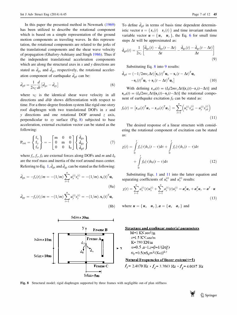
time. For a three-degree freedom system like rigid one-story

roof diaphragm with two translational DOFs in x and

y directions and one rotational DOF around z axis,

perpendicular to xy surface (Fig. 8) subjected to base

acceleration, external excitation vector can be stated as the

following:

Pext ¼fx

fy

fh

8<

:

9=

; ¼ �m 0 0

0 m 0

0 0 I0

24

35

€dgx

€dgy

€dgh

8<

:

9=

; ð7Þ

where fx, fy, fh are external forces along DOFs and m and I0

are the roof mass and inertia of the roof around mass center.

Referring to Eq. 1, €dgx and €dgy can be stated as the following:

€dgx ¼ �fx tð Þ=m ¼ � 1=mð ÞXn

i¼1

u ið Þx s ið Þ

x ¼ � 1=mð Þ: sx tð ÞT ux

ð8aÞ

€dgy ¼ �fy tð Þ=m ¼ � 1=mð ÞXn

i¼1

u ið Þy s ið Þ

y ¼ � 1=mð Þ: sy tð ÞT uy

ð8bÞ

To define €dgh in terms of basis time dependent determin-

istic vector s ¼ sx tð Þ sy tð Þf g and time invariant random

variable vector u ¼ ux uyf g, the Eq. 6 for small time

steps Dt will be approximated as:

€dgh tð Þ ¼ 1

2vc

€dgx tð Þ � €dgx t � Dtð ÞDt

�€dgy tð Þ � €dgy t � Dtð Þ

Dt

� �

ð9Þ

Substituting Eq. 8 into 9 results:

€dgh ¼ �1=2mvcDtð Þ sx tð ÞT ux � sx t � Dtð ÞT ux

�

�sy tð ÞT uy þ sy t � Dtð ÞT uy

�ð10Þ

With defining sxh(t) = (I0/2mvcDt)[sx(t)-sx(t-Dt)] and

syh(t) = (I0/2mvcDt)[sy(t)-sy(t-Dt)] the rotational compo-

nent of earthquake excitation fh can be stated as:

fh tð Þ ¼ sxh tð ÞT ux � syh tð ÞT uy

� �¼

Xn

i¼1

u ið Þx s

ið Þxh � u ið Þ

y sið Þ

yh

� �

ð11Þ

The desired response of a linear structure with consid-

ering the rotational component of excitation can be stated

as:

v tð Þ ¼Z t

0

fx sð Þhx t � sð Þds þZ t

0

fy sð Þhy t � sð Þds

þZ t

0

fh sð Þhh t � sð Þds ð12Þ

Substituting Eqs. 1 and 11 into the latter equation and

separating coefficients of ux(i) and uy

(i) results:

v tð Þ ¼Xn

i¼1

a ið Þx tð Þu ið Þ

x þXn

i¼1

a ið Þy tð Þu ið Þ

y ¼ aTx ux þ aT

y uy ¼ aT � u

ð13Þ

where u ¼ ux uyf g; a ¼ ax ayf g and

Fig. 8 Structural model; rigid diaphragm supported by three frames with negligible out-of plan stiffness


123

a ið Þx tð Þ ¼

Z t

0

sðiÞx sð Þhx t � sð Þ þ sðiÞxh sð Þhh t � sð Þ

n ods ð14aÞ

a ið Þy tð Þ ¼

Z t

0

sðiÞy sð Þhy t � sð Þ � sðiÞyh sð Þhh t � sð Þ

n ods ð14bÞ

For nonlinear problems again we can solve the optimi-

zation problem and find the design point u�. After finding

design point excitation the gradient vector of the linearized

limit state surface can be obtained from Eq. 4. The

obtained vector separated to 2 vectors ax and ay each with n

elements. The result of approximating Eqs. 14a and 14b

integrals with simple rectangular rule is as:

Xn

j¼1

s ið Þx tj

� h

ið Þxh tn � tj�

Dt ¼ a ið Þx tð Þ i ¼ 1; . . .; n ð15aÞ

Xn

j¼1

s ið Þy tj

� h

ið Þyh tn � tj�

Dt ¼ a ið Þy tð Þ i ¼ 1; . . .; n ð15bÞ

where

hið Þ

xh tn � tj

� ¼ hx tn � tj

� þ hh tn � tj

� sðiÞxh tj

� =sðiÞx tj

� � �

ð16aÞ

hið Þ

yh tn � tj

� ¼ hy tn � tj

� � hh tn � tj

� sðiÞyh tj

� =sðiÞy tj

� � �

ð16bÞ

If the external force was filtered white noise excitation

in the two directions because the presence of sið Þ

xh tj

� =s

ðiÞx tj

�

and sið Þ

yh tj

� =s ið Þ

y tj

� terms which are dependent to i, solving

Eq. 15 for obtaining hxh(i)(tn-tj) and h

ið Þyh tn � tj�

is difficult

or maybe impossible. But for white noise excitations if Sx

and Sy are spectral intensity in x and y directions, respec-

tively, the values of elements of vectors sy t ¼ i � Dtð Þ and

sy t ¼ i � Dtð Þ are zero, except the ith elements of these

vectors which are equal to rx ¼ffiffiffiffiffiffiffiffiffiffiffiffiffiffi2pSxDt

pand

rY ¼ffiffiffiffiffiffiffiffiffiffiffiffiffiffi2pSyDt

p, respectively. Thus the horizontal and

rotational components at time t ¼ i � Dt i.e. the ith ele-

ments of load vector are as the following:

fx tð Þ ¼ mrxuðiÞx ð17aÞ

fy tð Þ ¼ mryuðiÞy ð17bÞ

fh tð Þ ¼ mrxh uðiÞx � uði�1Þ

x

� �� mryh uðiÞ

y � uði�1Þy

� �ð17cÞ

where rxh ¼ I0=2vcDtð Þrx and ryh ¼ I0=2vcDtð Þry. After

substituting Eq. 17a, 17b, 17c into 14a, 14b and using

rectangular rule for Duhamel’s integral and with a little

simplification we have:

v tð Þ ¼Xn

i¼1

mrxhið Þ

xh u ið Þx Dt þ

Xn

i¼1

mryhið Þ

yh u ið Þy Dt ð18Þ

where hið Þ

xh ¼ h ið Þx þ I0=2mvcDtð Þ h

ið Þh � h

iþ1ð Þh

� �and h

ið Þyh ¼

h ið Þy � I0=2mvcDtð Þ h

ið Þh � h

iþ1ð Þh

� �, h ið Þ

x ¼ hx t � tið Þ, h ið Þy ¼

hy t � tið Þ and hið Þ

h ¼ hh t � tið Þ. Thus the values of hðiÞxh and

hðiÞyh could be obtained as follows:

hðiÞxh ¼ a ið Þ

x =mrxDt; hðiÞyh ¼ a ið Þ

y =mryDt ð19Þ

Therefore, the equivalent linear system is defined by two

IRFs which are affected by the presence of dependent

rotational component.

It is worthy of note that the presented method for sim-

ulating the dependent rotational component is a rough

proposal method. To obtain a more precise method it is

required to compare the simulated component with real

database of earthquake and match the results. In the con-

tinuation of this paper to investigate the application of the

proposed method in TELM analysis a numerical example

has been presented.

Example 3 A3D structure with a rigid roof diaphragm

which is supported by two frames in x and one frame in

y direction as shown in Fig. 8 is considered. The out-of

plane stiffness and damping of frames are negligible. The

in-plane internal force of frames is stated by non-degrading

uni-axial Bouc–Wen model (‘‘Appendix A’’). The initial

stiffness, K, damping, c, and Bouc–Wen properties of all

frames are identical and have been shown in Fig. 8. The

frames are massless and the mass of the rigid diaphragm

M and natural frequencies of system are also shown in this

Figure.

Excitation is independent bi-directional white noise base

acceleration with identical spectral intensity in x and y

directions with S0 ¼ 1 m2=s3. Furthermore the duration of

the excitation is set as tn = 6 s.

The dimensions of roof diaphragm are b ¼ Sdim � 30 m,

d ¼ Sdim � 20 m and the eccentricities of the frame A is

e ¼ Sdim � 5 m, where Sdim is the scale parameter for

considering systems with different dimension without

changing in the natural frequencies of the system. The

desired response is displacement of frame C in the

x direction.

Even though the frequency content of excitations is

dependent on the soil type and shear wave velocity, but in

this study only wide band white noise translational exci-

tation without considering the effects of soil properties is

used for extending TELM with dependent rotational

component.


123

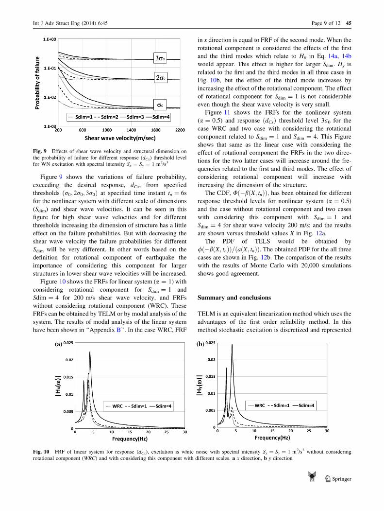
Figure 9 shows the variations of failure probability,

exceeding the desired response, dCx, from specified

thresholds r0; 2r0; 3r0ð Þ at specified time instant tn ¼ 6s

for the nonlinear system with different scale of dimensions

(Sdim) and shear wave velocities. It can be seen in this

figure for high shear wave velocities and for different

thresholds increasing the dimension of structure has a little

effect on the failure probabilities. But with decreasing the

shear wave velocity the failure probabilities for different

Sdim will be very different. In other words based on the

definition for rotational component of earthquake the

importance of considering this component for larger

structures in lower shear wave velocities will be increased.

Figure 10 shows the FRFs for linear system (a = 1) with

considering rotational component for Sdim = 1 and

Sdim = 4 for 200 m/s shear wave velocity, and FRFs

without considering rotational component (WRC). These

FRFs can be obtained by TELM or by modal analysis of the

system. The results of modal analysis of the linear system

have been shown in ‘‘Appendix B’’. In the case WRC, FRF

in x direction is equal to FRF of the second mode. When the

rotational component is considered the effects of the first

and the third modes which relate to Hh in Eq. 14a, 14b

would appear. This effect is higher for larger Sdim. Hy is

related to the first and the third modes in all three cases in

Fig. 10b, but the effect of the third mode increases by

increasing the effect of the rotational component. The effect

of rotational component for Sdim = 1 is not considerable

even though the shear wave velocity is very small.

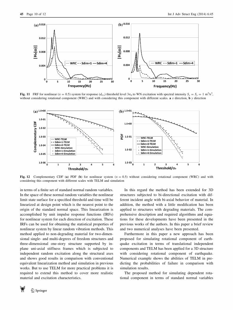
Figure 11 shows the FRFs for the nonlinear system

(a = 0.5) and response ðdCxÞ threshold level 3r0 for the

case WRC and two case with considering the rotational

component related to Sdim = 1 and Sdim = 4. This Figure

shows that same as the linear case with considering the

effect of rotational component the FRFs in the two direc-

tions for the two latter cases will increase around the fre-

quencies related to the first and third modes. The effect of

considering rotational component will increase with

increasing the dimension of the structure.

The CDF, U �b X; tnð Þð Þ; has been obtained for different

response threshold levels for nonlinear system (a = 0.5)

and the case without rotational component and two cases

with considering this component with Sdim = 1 and

Sdim = 4 for shear wave velocity 200 m/s; and the results

are shown versus threshold values X in Fig. 12a.

The PDF of TELS would be obtained by

/ �b X; tnð Þð Þ= a X; tnð Þð Þ. The obtained PDF for the all three

cases are shown in Fig. 12b. The comparison of the results

with the results of Monte Carlo with 20,000 simulations

shows good agreement.

Summary and conclusions

TELM is an equivalent linearization method which uses the

advantages of the first order reliability method. In this

method stochastic excitation is discretized and represented

Fig. 9 Effects of shear wave velocity and structural dimension on

the probability of failure for different response (dCx) threshold level

for WN excitation with spectral intensity Sx = Sy = 1 m2/s3

Fig. 10 FRF of linear system for response (dCx), excitation is white noise with spectral intensity Sx = Sy = 1 m2/s3 without considering

rotational component (WRC) and with considering this component with different scales. a x direction, b y direction


123

in terms of a finite set of standard normal random variables.

In the space of these normal random variables the nonlinear

limit state surface for a specified threshold and time will be

linearized at design point which is the nearest point to the

origin of the standard normal space. This linearization is

accomplished by unit impulse response functions (IRFs)

for nonlinear system for each direction of excitation. These

IRFs can be used for obtaining the statistical properties of

nonlinear system by linear random vibration methods. This

method applied to non-degrading material for two-dimen-

sional single- and multi-degrees of freedom structures and

three-dimensional one-story structure supported by in-

plane uni-axial stiffness frames which is subjected to

independent random excitation along the structural axes

and shows good results in comparison with conventional

equivalent linearization method and simulation in previous

works. But to use TELM for more practical problems it is

required to extend this method to cover more realistic

material and excitation characteristics.

In this regard the method has been extended for 3D

structures subjected to bi-directional excitation with dif-

ferent incident angle with bi-axial behavior of material. In

addition, the method with a little modification has been

applied to structures with degrading materials. The com-

prehensive description and required algorithms and equa-

tions for these developments have been presented in the

previous works of the authors. In this paper a brief review

and two numerical analyses have been presented.

Furthermore in this paper a new approach has been

proposed for simulating rotational component of earth-

quake excitation in terms of translational independent

components and TELM has been applied for a 3D structure

with considering rotational component of earthquake.

Numerical example shows the abilities of TELM in pre-

dicting the probabilities of failure in comparison with

simulation results.

The proposed method for simulating dependent rota-

tional component in terms of standard normal variables

Fig. 11 FRF for nonlinear (a = 0.5) system for response (dCx) threshold level 3r0 to WN excitation with spectral intensity Sx = Sy = 1 m2/s3,

without considering rotational component (WRC) and with considering this component with different scales. a x direction, b y direction

Fig. 12 Complementary CDF (a) PDF (b) for nonlinear system (a = 0.5) without considering rotational component (WRC) and with

considering this component with different scales with TELM and simulation


123

should be checked and calibrated with real rotational

component of earthquake in future works.

More investigations are needed to further generalize

TELM; some of these have been listed below:

• In finding the design point it is required to find the

response and its sensitivity with direct differentiation

method, this is the most challenging part of TELM, thus

developing the sensitivity analysis for using the other

material models is necessary.

• TELM in present and previous works have been only

applied to 2D stick-like models or shear beam models

or 3D models with rigid diaphragm supported by

nonlinear columns or frames. It is required to develop

this method for more general nonlinear systems

including frames with nonlinear beam and columns

and using models capable of predicting the dominant

yield pattern under random excitations.

• Developing of TELM for degrading material has been

done only for uni-axial Bouc–Wenn model, it is

required to consider this behavior for bi-axial materials

too.

• In the all previous works the excitation had been white

noise or modulated filtered white noise, using simulated

real earthquakes as inputs would be a good subject for

research.

• The considered response in all the previous works had

been displacement response, investigating about other

response quantities such as forces, moments and

application of damage indexes would be interesting.

• Finally application of the TELM in performance-based

assessment and design framework would be the subject

of future investigations.

Acknowledgments The Authors express their appreciation to Prof.

A. Der Kiureghian for his valuable help and comments for this study.

Open Access This article is distributed under the terms of the

Creative Commons Attribution License which permits any use, dis-

tribution, and reproduction in any medium, provided the original

author(s) and the source are credited.

Appendix A: Bouc–Wen material model

Uni-axial Bouc–Wen model

Bouc–Wen class models have been widely used to effi-

ciently describe smooth hysteretic behavior in time history

and random vibration analyses (Song and Der Kiureghian

2006). This model which in the first time presented for

modeling uni-axial non-degrading hysteretic behavior by

Bouc (1967) was generalized and used in nonlinear random

vibration in Wen (1976), this model by adding new

parameters developed for considering stiffness and strength

degradation in Baber and Wen (1981). Even though this

model was developed for considering pinching behavior of

materials in Baber and Noori (1986) the model of Baber

and Wen (1981) has been considered in this paper and

pinching behavior has been eliminated.

The nonlinear restoring force in Bouc–Wen model can

be stated as the following for each nonlinear elements of

the model:

Pint tð Þ ¼ aKd tð Þ þ 1 � að ÞKz tð Þ ð20Þ

where Pint is the nonlinear hysteretic force, d is the relative

displacement of nonlinear element, K is the initial stiffness,

a is the ratio of the yielding stiffness to the initial stiffness

and z is the hysteretic component of displacement:

_z ¼ 1=gð Þ _d � m b _d�� zj jn̂�1

z þ c _d zj jn̂� �n o

ð21Þ

In the above relation dot shows the derivative with

respect to time. c, b and n̂ are parameters that control the

basic hysteretic shape, m and g are, respectively, strength

and stiffness degradation shape functions and define as the

following:

mðeÞ ¼ 1 þ dme ð22ÞgðeÞ ¼ 1 þ dge ð23Þ

where dm and dg, respectively, determine the rate of

strength and stiffness degradations. Strength and stiffness

degradation are controlled by the hysteretic energy

dissipation e that be defined as:

e ¼ 1 � að ÞKZ t

0

z _udt ð24Þ

For non-degrading case dm and dg are zeros.

Bi-axial Bouc–Wen

In the bi-axial Bouc–Wen model (Park et al. 1986; Wen

and Yeh 1989) restoring force in x and y directions is as

follows:

Pintx;Pinty

� T¼ a Kxdx;Kydy

� Tþ 1 � að Þ Kxzx;Kyzy

� T

ð25Þ

where Kx and Ky are initial stiffness coefficients; zx and zy

are hysteretic components of displacement of element,

respectively, in x and y directions and a is the ratio of

stiffness after yielding to the initial stiffness. Hysteretic

components of displacement can be stated as the

following:


123

_zx ¼ _dx � zx_dx

�� zxj jn̂�1 b þ csgn _dxzx

� � �

� zx_dy

�� zy

�� n̂�1b þ csgn _dyzy

� � �

_zy ¼ _dy � zy_dx

�� zxj jn̂�1 b þ csgn _dxzx

� � �

� zy_dy

�� zy

�� n̂�1b þ csgn _dyzy

� � �

ð26Þ

where sgnð:Þ is the sign function.

c and b are constant parameters of the model and control

the shape of hysteresis loops. Furthermore, n̂ is a natural

number parameter that represents the yield surface or rate

of bi-axial interaction. If n̂ ¼ 1 the yield surface becomes a

rhombus and implies very significant interaction and with

increasing n̂ the effect of interaction decreases. For n̂ ¼ 2

the yield surface for isotropic case is a circle that represents

equal yield capacity along any direction and with further

increasing as n approaches infinity, the yield surface

becomes a square and the yield strength along one axis is

independent of the displacement along its orthogonal axis

(Lee and Hong 2010).

Appendix B: Relation between the modal IRFs

and the IRFs in the directions of the excitations

With considering degrees of freedom as dx, dy and dh and

Sdim ¼ 1 mass, M, stiffness, K, and damping, C, matrices

are as the following:

M ¼1 0 0

0 1 0

0 0 1300=12

2

64

3

75;K ¼560 0 0

0 280 1400

0 1400 63000

2

64

3

75;

C ¼3 0 0

0 1:5 7:5

0 7:5 337:5

2

64

3

75

Eigenvalue and eigenvector matrices of this system are:

U ¼0 1 0

�0:9344 0 0:3562

0:0342 0 0:0898

264

375;

x2 ¼228:7206 0 0

0 560 0

0 0 632:8179

264

375

where x2 and U are eigenvalue and eigenvector matrices. For

the desired response v = dcx = dx ? (d/2)dh the relation

between impulse response function in the direction of DOFs

and modal IRFs, h1, h2, and h3 are as follows:

hx ¼ h2 tn � sð Þhy ¼ �0:3195648h1 tn � sð Þ þ 0:3198676h3 tn � sð Þf g

hh ¼ 0:0116964h1 tn � sð Þ þ 0:0806404h3 tn � sð Þf g

To obtain hxh and hyh it is required to obtain the above

relations into Eq. 16a, 16b.

References

Baber TT, Noori MN (1986) Modeling general hysteretic behavior

and random vibration application. ASME J Vib Acoust Stress

Reliab Des 108:411–420

Baber TT, Wen YK (1981) Random vibration of hysteretic degrading

systems. J Eng Mech 107:1069–1087

Bouc R (1967) Forced vibration of mechanical systems with

hysteresis. In: Proceedings of the 4th conference of nonlinear

oscillations, Prague, Czechoslovakia, p 315

Broccardo M, Der Kiureghian A (2012) Multi-component nonlinear

stochastic dynamic analysis using tail-equivalent linearization

method. In: Proceeding of 15th world conference on earthquake

engineering, September, Lisbon, Portugal

Der Kiureghian A, Fujimura K (2009) Nonlinear stochastic dynamic

analysis for performance-based earthquake engineering. Earth-

quake Eng Struct Dynam 38:719–738

Fujimura K, Der Kiureghian A (2007) Tail equivalent linearization

method for nonlinear random vibration. Probab Eng Mech

22:63–76

Ghafory-Ashtiany M, Raoofi R (2013) Nonlinear bi-axial structural

vibration under bi-directional random excitation by Tail Equiv-

alent Linearization Method. Part II: excitation with incident

angle h, (under preparation)

Ghafory-Ashtiany M, Singh MP (1986) Structural response for six

correlated earthquake component. 14:101–19

Lee CS, Hong HP (2010) Statistics of inelastic response of hysteretic

systems under bi-directional seismic excitations. Eng Struct,

322074–2086

Newmark NM (1969) Torsion in symmetrical building’. In: Proceed-

ings of the 4th world conference of earthquake engineering.

Santiago, Chile 2. A.3, 19–32

Park YJ, Wen YK, H-S Ang A (1986) Random vibration of hysteretic

systems under bi-directional ground motion. Earthquake Eng

Struct Dynam 14:543–557

Penzien J, Watabe M (1975) Characteristics of 3-dimensional

earthquake ground motions. Earthquake Eng Struct Dynam

3:365–373

Raoofi R, Ghafory-Ashtiany M (2013a) Nonlinear bi-axial structural

vibration under bi-directional random excitation by Tail Equiv-

alent Linearization Method. Part I: excitation along the structural

axes, (under preparation)

Raoofi R, Ghafory-Ashtiany M (2013b) Random vibration of

nonlinear structures with stiffness and strength deterioration by

modified tail equivalent linearization method, (under

preparation)

Rezaeian S, Der Kirureghian A (2011) Simulation of orthogonal

horizontal ground motion components for specified earthquake

and site characteristics. Earthquake Eng Struct Dynam

41:335–353

Singh MP, Ghafory-Ashtiany M (1984) Structural response under

multicomponent earthquake. J Eng Mech Div ASCE

110:761–775

Song J, Der Kiureghian A (2006) Generalized Bouc–Wen model for

highly asymmetric hysteresis. Eng Mech 132(6):610–618

Wen YK (1976) Method for random vibration of hysteretic systems.

Eng Mech Division 102(2):249–263

Wen YK, Yeh CH (1989) Bi-axial and torsional response of inelastic

structures under random excitation. Struct Saf 6:137–152


123

nonlinear random vibration using updated tail equivalent ... · nonlinear random vibration using...

Documents