nonlinear elliptic-parabolic - gwdgwebdoc.sub.gwdg.de/ebook/dissts/duisburg/jakubowski2002.pdf ·...
TRANSCRIPT
Nonlinear elliptic-parabolic
integro-differential equations with L1-data:
existence, uniqueness, asymptotics
DISSERTATION
zur Erlangung des akademischen Grades eines
Doktors der Naturwissenschaften
dem Fachbereich Mathematik und Informatik
der Universitat Essen
vorgelegt von
Volker G. Jakubowski
geboren in Wanne-Eickel
Juli 2001
Dekan Prof. Dr. Dieter Lutz
Gutachter Prof. Dr. Stig-Olof Londen, Helsinki
Prof. Dr. Jan Pruss, Halle
Prof. Dr. Wolfgang Ruess, Essen
Tag der mundlichen Prufung 24.04.2002
Contents
1 Introduction 5
1.1 Diffusion of fluids in porous media with memory . . . . . . . . . . . . . . . 10
1.2 Heat flow in materials with memory . . . . . . . . . . . . . . . . . . . . . . 11
1.3 Abstract Volterra equations . . . . . . . . . . . . . . . . . . . . . . . . . . 15
2 Regularity of solutions 19
2.1 Continuity of solutions . . . . . . . . . . . . . . . . . . . . . . . . . . . . . 20
2.2 Strong solutions . . . . . . . . . . . . . . . . . . . . . . . . . . . . . . . . . 29
3 Entropy solutions 45
3.1 Nonexistence and nonuniqueness of weak solutions . . . . . . . . . . . . . . 52
3.2 A Kato inequality . . . . . . . . . . . . . . . . . . . . . . . . . . . . . . . . 60
3.3 Uniqueness of entropy solutions . . . . . . . . . . . . . . . . . . . . . . . . 71
3.4 Existence of entropy solutions . . . . . . . . . . . . . . . . . . . . . . . . . 83
4 Asymptotic behavior 105
4.1 Asymptotic almost periodicity . . . . . . . . . . . . . . . . . . . . . . . . . 108
4.2 The limit equation . . . . . . . . . . . . . . . . . . . . . . . . . . . . . . . 113
4.3 Eberlein-weak almost periodicity . . . . . . . . . . . . . . . . . . . . . . . 120
A Complete Positivity 133
B Accretivity 141
References 146
3

4
Chapter 1
Introduction
In this thesis we consider the history dependent initial-boundary value problem
∂
∂t
(κ(b(v(t, x))− b(v0(x))
)+
∫ t
0
k(t− s)(b(v(s, x))− b(v0(x))
)ds)
= div a(x,Dv(t, x)) + f(t, x) for (t, x) ∈ Q := (0, T )× Ω,
b(v)(0, ·) = b(v0) in Ω,
v(t, x) = 0 for (t, x) ∈ Γ := (0, T )× ∂Ω
(1.1)
in a bounded domain Ω ⊂ RN . We assume that a : Ω × RN → RN is a Caratheodory
function satisfying the classical Leray-Lions conditions which defines a bounded continuous
coercive operator from W 1,p0 (Ω) into its dual space for some 1 < p < ∞. However, some
of our results will also apply to (1.1) with the operator − div a(x,Dv) replaced by the
operator − div a(x, v,Dv), and some will even be applicable to conservation laws with
memory. Additionally, we impose the following assumptions on κ, k and b.
κ ≥ 0 and k : (0,∞) → R is a nonnegative, nonincreasing function such that
k ∈ L1loc([0,∞)) and κ+
∫ t
0k(s) ds > 0 for all t > 0.
(1.2)
b : R → R is continuous and nondecreasing, satisfying the normalization con-
dition b(0) = 0.(1.3)
Note that these assumptions are quite general. As a special case, the degenerated elliptic-
parabolic initial boundary value problem
b(v)t = div a(x,Dv) + f in Q,
b(v)(0, ·) = b(v0) in Ω,
v = 0 on Γ,
(1.4)
5
6 CHAPTER 1. INTRODUCTION
is included. Defining κ = 0 and k(t) := t−γ/Γ(1−γ), one easily sees that our assumptions
also include the case of a fractional derivative of order 0 < γ < 1 in time, i.e.
∂γ
∂tγb(v) = div a(x,Dv) + f in Q,
b(v)(0, ·) = b(v0) in Ω,
v = 0 on Γ.
(1.5)
Here, the fractional derivative of order 0 < γ < 1 is defined by
∂γ
∂tγu(t) :=
∂
∂t
∫ t
0
(t− s)−γ
Γ(1− γ)u(s) ds, t > 0,
∂γ
∂tγu(0) :=
1
hlim
h→0+
∫ h
0
(h− s)−γ
Γ(1− γ)u(s) ds,
(1.6)
where u ∈ C([0, T ];L1(Ω)) satisfying u(0, ·) = 0, c.f. [Zyg59, Chapter XII.8].
We recall that equations of the form (1.4) and (1.5) are obtained when modelling the
transport of fluids in porous media. For the fractional derivative case (1.5), we refer to
[Cap99, Cap00] and the references therein. Indeed, in geothermal areas the fluid may
precipitate minerals in the pores of the medium, thus diminishing their size. To study
such situations, Darcy’s law has to be modified inducing a memory term. As shown in
[Cap99], this leads to a formulation as in (1.5) for 0 < γ < 1.
But also the case κ > 0 and k 6≡ 0 is of particular interest. Indeed, a second application
for (1.1) is the nonlinear heat flow in certain dielectric materials at very low temperatures.
In this situation, finite speed of propagation of thermal disturbances has been observed
experimentally. Several models to describe this phenomenon have been introduced. In
particular, [GP68, Mac77] and [Nun71] introduce a model in which the constitutive rela-
tions for the internal energy and heat flux, in difference to Fourier’s law, also depend on
the history of the temperature and the temperature gradient, respectively. As shown in
[CN81], this yields a problem of the form (1.1) under certain assumptions on the internal
energy and heat flux relaxation functions.
We remark that the assumptions on κ, k in (1.2) are motivated by the fact that one wants
to insure positivity of solutions. In several applications this is a physically necessary
assumption. Indeed, when modelling the nonlinear heat flow in materials with memory
one assumes v(t, x) of problem (1.1) to denote the absolute temperature in x ∈ Ω at time
t. Such assumptions were first introduced in [CN79] and lead to the notion of complete
positivity, c.f. [CN81] and [CM88].
It is our intention to develop a solution theory for (1.1) in the state space L1(Ω). Indeed, as
the space L1(Ω) is the natural setting for several evolution problems, such as the transport
of fluids in porous media and heat conduction, we are interested in solving (1.1) for general
7
L1-data, i.e. for
v0 : Ω → R measurable with b(v0) ∈ L1(Ω),
f ∈ L1(Q).
We recall that the case of the elliptic problem
b(v) = div a(x,Dv) + f in Ω,
v = 0 on ∂Ω,(1.7)
and of the elliptic-parabolic problem (1.4) with general L1-data has been investigated by
several authors in recent years. Note that, when considering weak solutions, i.e. solutions
in the sense of distributions, of (1.7) and (1.4), respectively, one encounters a problem of
nonexistence of solutions for small p, i.e., for 1 < p < 2 − 1N
, see [BBG+95, Appendix
I]. Moreover, as shown in a counterexample given in [Ser64] for a linear problem, weak
solutions are in general not unique. These problems of nonexistence and nonuniqueness
of weak solutions carry over to the history dependent case.
In order to overcome the above mentioned problems of nonexistence and nonuniqueness of
weak solutions, new notions of solutions for the elliptic and the elliptic-parabolic problem,
i.e. for (1.7) and (1.4), have been introduced. One concept to guarantee uniqueness is
the concept of renormalized solutions, which was first introduced in [DL89] for the study
of the Boltzmann equation. In [BGDM93] and [Mur93], this concept was then applied
to an elliptic problem, and was extended to parabolic problems in [BM97]. The second
concept, which can be shown to be equivalent to the concept of renormalized solutions
for the elliptic and parabolic problems, is the concept of entropy solutions introduced in
[BBG+95]. See also [AMSdLT99] for the extension to parabolic equations.
We compare the two concepts of solutions in order to develop a solution theory for the
history dependent degenerated elliptic-parabolic problem (1.1) in the state space L1(Ω).
It turns out that only the notion of entropy solutions can naturally be extended to our
problem (1.1) for general κ, k satisfying (1.2). This is due to the fact that the derivative
in time operator in (1.1) does not satisfy a Kato equality, but only a Kato inequality. For
the new notion of entropy solutions of (1.1) that we introduce, existence and uniqueness
of solutions are shown under certain assumptions.
It turns out that the notion of entropy solutions of (1.1) coincides for u = b(v) and
u0 = b(v0) with the notion of generalized solutions, see [Gri85, CGL96], of the abstract
Volterra equation
d
dt
(κ(u(t)− u0) +
∫ t
0
k(t− s)(u(s)− u0) ds
)+ Au(t) 3 f(t), t ∈ [0, T ) (1.8)
in L1(Ω). Here, A is an m-accretive, or m-completely accretive, possibly multivalued,
operator in L1(Ω) corresponding to b and − div a(x,Dv).
8 CHAPTER 1. INTRODUCTION
Moreover, we investigate the regularity of solutions by considering generalized solutions of
the abstract Volterra equation (1.8). As shown in [Gri85], the existence of strong solutions
of (1.8) can be obtained for κ = 0, even if the generalized solution itself is not differentiable
a.e. on the interval (0, T ). For κ > 0, this can not be achieved in general. Therefore,
we recall that for an arbitrary m-accretive operator A in a general real Banach space X,
Lipschitz continuity of the generalized solution u of (1.8) is known by [Gri85, Theorem 2]
if u0 ∈ D(A) and f ∈ BV ([0, T );X). Since the Radon-Nikodym property of the space X
is equivalent to the differentiability of absolutely continuous functions u : (0, T ) → X, we
can conclude that the generalized solution u of (1.8) is in fact a strong solution if X has
the Radon-Nikodym property and u0 ∈ D(A) and f ∈ BV (0, T ;X).
However, in spaces without the Radon-Nikodym property, such as L1(Ω), no general reg-
ularity results are known. In the case of κ > 0, we therefore restrict our investigation to
m-completely accretive operators A in a normal Banach space X ⊂ L1(Ω). We show that
under these assumptions regularity results can be achieved that are quite similar to those
known for accretive operators in Banach spaces having the Radon-Nikodym property.
One of the most important qualitative questions in evolution problems is the one on the
long-time behavior. One is interested in stability, the existence of equilibria, or periodic
solutions, or those which are close-to-periodic, such as asymptotically almost periodic
solutions, or weakly almost periodic solutions in the sense of Eberlein. The results obtained
here extend those of [Kre92, Kre96] for mild solutions of nonlinear Cauchy problems and
those of [CN81] on nonlinear Volterra equations. We give sufficient conditions such that the
generalized solution of (1.8) is asymptotically almost periodic, respectively weakly almost
periodic in the sense of Eberlein. Since, in applications, one is often only interested in the
asymptotic behavior of the mean of the solution, we give a characterization of the almost
periodic part of the generalized solution as a solution of a certain limit equation. Here,
we only assume that the operator A is m-accretive. Thus, the results obtained apply to
(1.1) as well as to conservation laws with memory as considered in [CGL96].
In chapter 2 we consider the regularity of generalized solutions of the abstract Volterra
equation (1.8). The main tool is an integral inequality developed in section 2.1, see proposi-
tion 2.1, allowing us to compare two generalized solutions for different data. The remainder
of section 2.1 is devoted to simple applications of this integral inequality. In section 2.2 we
investigate the existence of strong solutions of (1.8) in Banach spaces without the Radon-
Nikodym property. Our main result is given in proposition 2.14, stating the existence of
strong solutions for m-completely accretive operators in normal Banach spaces X ⊂ L1(Ω)
satisfying a strong convergence condition. This result is essential for the existence of weak
solutions of (1.1) for regular data.
In chapter 3 we introduce a notion of entropy solutions for the history dependent degener-
ated elliptic-parabolic problem (1.1), see definition 3.3, and show existence and uniqueness
of solutions. Section 3.1 is concerned with the question of nonexistence and nonuniqueness
9
of weak solutions. In section 3.2 a Kato inequality for the time derivative operator in (1.1)
is developed, see proposition 3.23 and corollary 3.24. We also give a motivation for the
fact that the concept of renormalized solutions is not applicable in a straightforward way
in the context of (1.1). The uniqueness of entropy solutions is shown in section 3.3, see
theorem 3.26. An essential tool is Kruzhkov’s method of doubling variables, which was
first introduced in [Kru70]. Since we need some assumptions on the continuity of solu-
tions, the final uniqueness result, corollary 3.31, is a consequence of the existence result for
b ≡ id, theorem 3.30, presented in section 3.4. The remainder of section 3.4 is concerned
with open problems in the theory of entropy solutions, such as the strong convergence of
an approximating sequence of solutions in Lp(0, T ;W 1,p0 (Ω)) and the existence of entropy
solutions for general b 6≡ id.
Chapter 4 is concerned with the asymptotic behavior of generalized solutions of (1.8).
The main estimate used for the proof of existence of asymptotically almost periodic so-
lutions and of weakly almost periodic solutions in the sense of Eberlein is obtained in
proposition 4.2 of section 4.1. It is then applied to show that generalized solutions are
asymptotically almost periodic under certain assumptions, see theorem 4.10. In section
4.2 we construct a solution of a certain limit equation on the whole real line characterizing
the almost periodic part of solutions of the initial value problem (1.8), see theorems 4.11
and 4.20. Section 4.3 is devoted to the study of weakly almost periodic solutions in the
sense of Eberlein. Existence of such solutions is shown in theorems 4.16 and 4.19. A main
tool used in this section is Grothendieck’s double limit criterion for weak compactness in
(Cb(R+), ‖ ·‖∞), see [RS89, Theorem 2.1] for the Banach space valued version. We remark
that the results obtained apply to (1.1) as well as to conservation laws with memory.
We conclude this introductory chapter by the investigation of two applications, in which
equations of the type (1.1) naturally occur, and by stating preliminary results on the
abstract Volterra equation (1.8). The applications, diffusion of fluids in porous media
with memory and heat flow in materials with memory, are presented in section 1.1 and
section 1.2, respectively. The main facts on the abstract Volterra equation (1.8) are given
in section 1.3.
Acknowledgements
The work on this thesis has greatly been influenced by a number of researchers in the field.
First, I owe deep insights into various recent concepts of solutions of nonlinear partial
differential equations to the late Philippe Benilan (Besancon). I am greatly indebted to
Petra Wittbold (Strasbourg) for collaboration in the present work on entropy solutions, as
well as to Stig-Olof Londen (Helsinki) and to Jan Pruss (Halle) for most valuable guidance,
ideas, and discussions on Volterra equations and their solution theory.
It is a pleasure for me to thank my teacher and advisor Wolfgang Ruess for his collaboration
in the present work on the asymptotic behavior of solutions, as well as for his guidance
10 CHAPTER 1. INTRODUCTION
and encouragement in the course of this thesis.
Thanks are also due to DAAD (Deutscher Akademischer Austauschdienst). DAAD has
granted financial support to quite a number of my research contacts, such as various visits
to the universities of Besancon and Strasbourg (within the scope of the French-German
research program PROCOPE), as well as a research visit by Stig-Olof Londen to Essen
University.
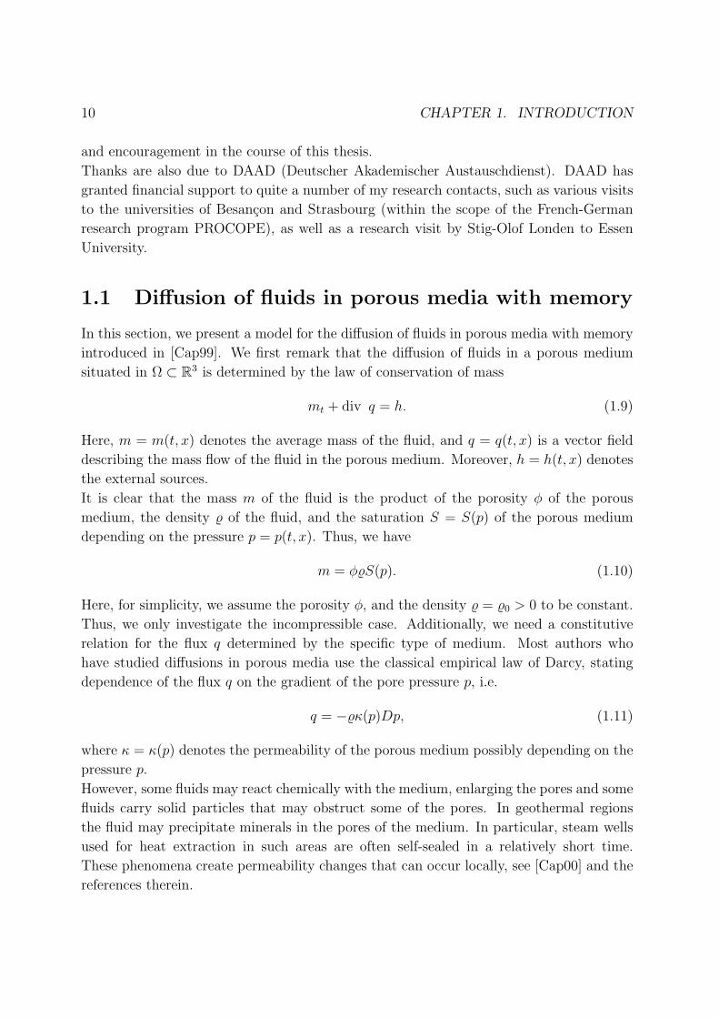
1.1 Diffusion of fluids in porous media with memory
In this section, we present a model for the diffusion of fluids in porous media with memory
introduced in [Cap99]. We first remark that the diffusion of fluids in a porous medium
situated in Ω ⊂ R3 is determined by the law of conservation of mass
mt + div q = h. (1.9)
Here, m = m(t, x) denotes the average mass of the fluid, and q = q(t, x) is a vector field
describing the mass flow of the fluid in the porous medium. Moreover, h = h(t, x) denotes
the external sources.
It is clear that the mass m of the fluid is the product of the porosity φ of the porous
medium, the density % of the fluid, and the saturation S = S(p) of the porous medium
depending on the pressure p = p(t, x). Thus, we have
m = φ%S(p). (1.10)
Here, for simplicity, we assume the porosity φ, and the density % = %0 > 0 to be constant.
Thus, we only investigate the incompressible case. Additionally, we need a constitutive
relation for the flux q determined by the specific type of medium. Most authors who
have studied diffusions in porous media use the classical empirical law of Darcy, stating
dependence of the flux q on the gradient of the pore pressure p, i.e.
q = −%κ(p)Dp, (1.11)
where κ = κ(p) denotes the permeability of the porous medium possibly depending on the
pressure p.
However, some fluids may react chemically with the medium, enlarging the pores and some
fluids carry solid particles that may obstruct some of the pores. In geothermal regions
the fluid may precipitate minerals in the pores of the medium. In particular, steam wells
used for heat extraction in such areas are often self-sealed in a relatively short time.
These phenomena create permeability changes that can occur locally, see [Cap00] and the
references therein.
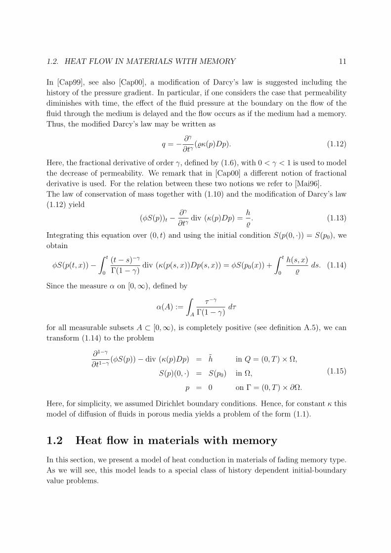
1.2. HEAT FLOW IN MATERIALS WITH MEMORY 11
In [Cap99], see also [Cap00], a modification of Darcy’s law is suggested including the
history of the pressure gradient. In particular, if one considers the case that permeability
diminishes with time, the effect of the fluid pressure at the boundary on the flow of the
fluid through the medium is delayed and the flow occurs as if the medium had a memory.
Thus, the modified Darcy’s law may be written as
q = − ∂γ
∂tγ(%κ(p)Dp). (1.12)
Here, the fractional derivative of order γ, defined by (1.6), with 0 < γ < 1 is used to model
the decrease of permeability. We remark that in [Cap00] a different notion of fractional
derivative is used. For the relation between these two notions we refer to [Mai96].
The law of conservation of mass together with (1.10) and the modification of Darcy’s law
(1.12) yield
(φS(p))t −∂γ
∂tγdiv (κ(p)Dp) =
h
%. (1.13)
Integrating this equation over (0, t) and using the initial condition S(p(0, ·)) = S(p0), we
obtain
φS(p(t, x))−∫ t
0
(t− s)−γ
Γ(1− γ)div (κ(p(s, x))Dp(s, x)) = φS(p0(x)) +
∫ t
0
h(s, x)
%ds. (1.14)
Since the measure α on [0,∞), defined by
α(A) :=
∫A
τ−γ
Γ(1− γ)dτ
for all measurable subsets A ⊂ [0,∞), is completely positive (see definition A.5), we can
transform (1.14) to the problem
∂1−γ
∂t1−γ(φS(p))− div (κ(p)Dp) = h in Q = (0, T )× Ω,
S(p)(0, ·) = S(p0) in Ω,
p = 0 on Γ = (0, T )× ∂Ω.
(1.15)
Here, for simplicity, we assumed Dirichlet boundary conditions. Hence, for constant κ this
model of diffusion of fluids in porous media yields a problem of the form (1.1).
1.2 Heat flow in materials with memory
In this section, we present a model of heat conduction in materials of fading memory type.
As we will see, this model leads to a special class of history dependent initial-boundary
value problems.
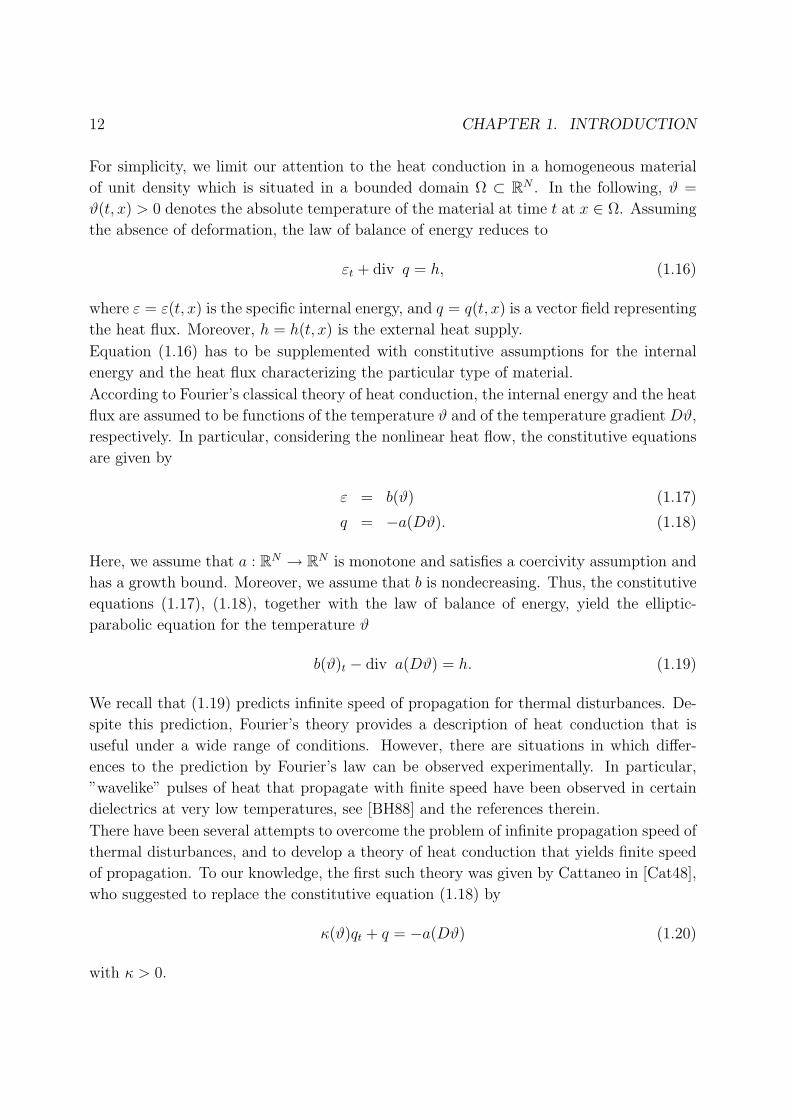
12 CHAPTER 1. INTRODUCTION
For simplicity, we limit our attention to the heat conduction in a homogeneous material
of unit density which is situated in a bounded domain Ω ⊂ RN . In the following, ϑ =
ϑ(t, x) > 0 denotes the absolute temperature of the material at time t at x ∈ Ω. Assuming
the absence of deformation, the law of balance of energy reduces to
εt + div q = h, (1.16)
where ε = ε(t, x) is the specific internal energy, and q = q(t, x) is a vector field representing
the heat flux. Moreover, h = h(t, x) is the external heat supply.
Equation (1.16) has to be supplemented with constitutive assumptions for the internal
energy and the heat flux characterizing the particular type of material.
According to Fourier’s classical theory of heat conduction, the internal energy and the heat
flux are assumed to be functions of the temperature ϑ and of the temperature gradient Dϑ,
respectively. In particular, considering the nonlinear heat flow, the constitutive equations
are given by
ε = b(ϑ) (1.17)
q = −a(Dϑ). (1.18)
Here, we assume that a : RN → RN is monotone and satisfies a coercivity assumption and
has a growth bound. Moreover, we assume that b is nondecreasing. Thus, the constitutive
equations (1.17), (1.18), together with the law of balance of energy, yield the elliptic-
parabolic equation for the temperature ϑ
b(ϑ)t − div a(Dϑ) = h. (1.19)
We recall that (1.19) predicts infinite speed of propagation for thermal disturbances. De-
spite this prediction, Fourier’s theory provides a description of heat conduction that is
useful under a wide range of conditions. However, there are situations in which differ-
ences to the prediction by Fourier’s law can be observed experimentally. In particular,
”wavelike” pulses of heat that propagate with finite speed have been observed in certain
dielectrics at very low temperatures, see [BH88] and the references therein.
There have been several attempts to overcome the problem of infinite propagation speed of
thermal disturbances, and to develop a theory of heat conduction that yields finite speed
of propagation. To our knowledge, the first such theory was given by Cattaneo in [Cat48],
who suggested to replace the constitutive equation (1.18) by
κ(ϑ)qt + q = −a(Dϑ) (1.20)
with κ > 0.
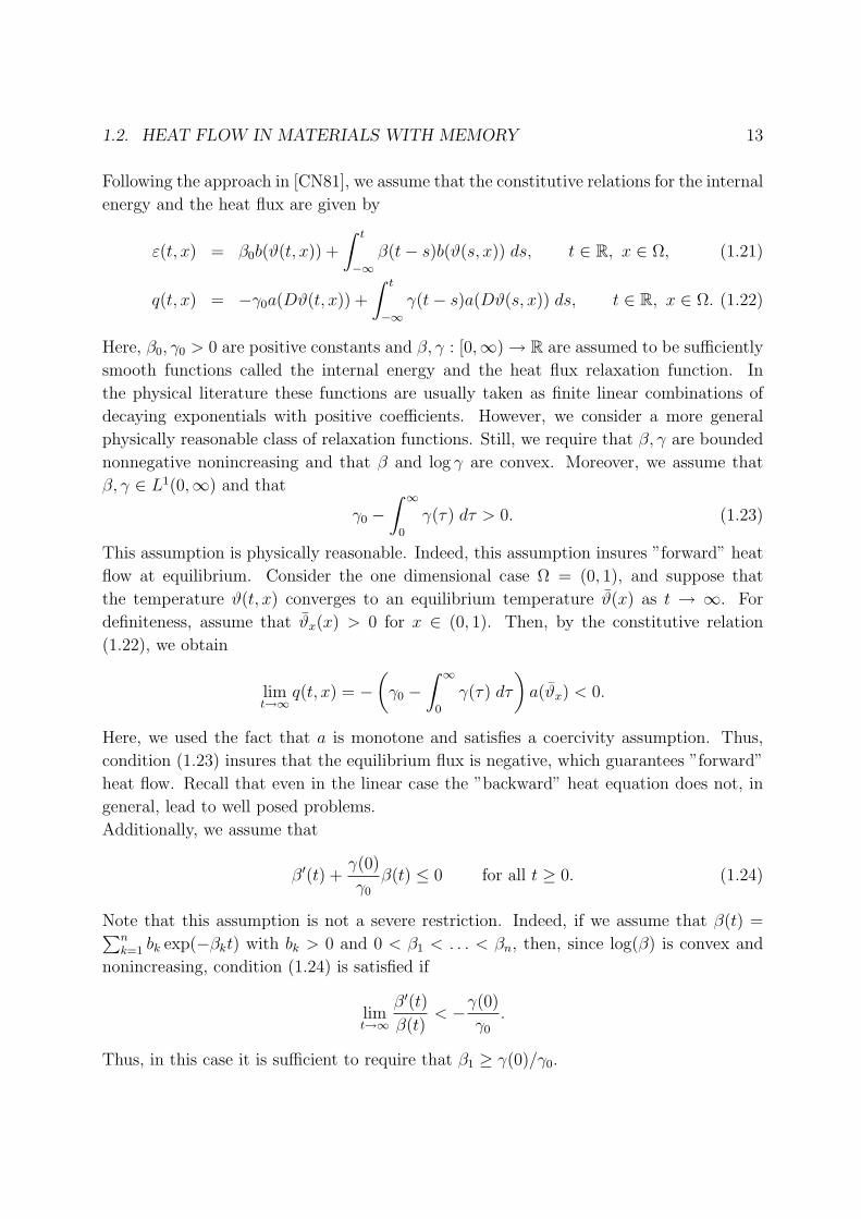
1.2. HEAT FLOW IN MATERIALS WITH MEMORY 13
Following the approach in [CN81], we assume that the constitutive relations for the internal
energy and the heat flux are given by
ε(t, x) = β0b(ϑ(t, x)) +
∫ t
−∞β(t− s)b(ϑ(s, x)) ds, t ∈ R, x ∈ Ω, (1.21)
q(t, x) = −γ0a(Dϑ(t, x)) +
∫ t
−∞γ(t− s)a(Dϑ(s, x)) ds, t ∈ R, x ∈ Ω. (1.22)
Here, β0, γ0 > 0 are positive constants and β, γ : [0,∞) → R are assumed to be sufficiently
smooth functions called the internal energy and the heat flux relaxation function. In
the physical literature these functions are usually taken as finite linear combinations of
decaying exponentials with positive coefficients. However, we consider a more general
physically reasonable class of relaxation functions. Still, we require that β, γ are bounded
nonnegative nonincreasing and that β and log γ are convex. Moreover, we assume that
β, γ ∈ L1(0,∞) and that
γ0 −∫ ∞
0
γ(τ) dτ > 0. (1.23)
This assumption is physically reasonable. Indeed, this assumption insures ”forward” heat
flow at equilibrium. Consider the one dimensional case Ω = (0, 1), and suppose that
the temperature ϑ(t, x) converges to an equilibrium temperature ϑ(x) as t → ∞. For
definiteness, assume that ϑx(x) > 0 for x ∈ (0, 1). Then, by the constitutive relation
(1.22), we obtain
limt→∞
q(t, x) = −(γ0 −
∫ ∞
0
γ(τ) dτ
)a(ϑx) < 0.
Here, we used the fact that a is monotone and satisfies a coercivity assumption. Thus,
condition (1.23) insures that the equilibrium flux is negative, which guarantees ”forward”
heat flow. Recall that even in the linear case the ”backward” heat equation does not, in
general, lead to well posed problems.
Additionally, we assume that
β′(t) +γ(0)
γ0
β(t) ≤ 0 for all t ≥ 0. (1.24)
Note that this assumption is not a severe restriction. Indeed, if we assume that β(t) =∑nk=1 bk exp(−βkt) with bk > 0 and 0 < β1 < . . . < βn, then, since log(β) is convex and
nonincreasing, condition (1.24) is satisfied if
limt→∞
β′(t)
β(t)< −γ(0)
γ0
.
Thus, in this case it is sufficient to require that β1 ≥ γ(0)/γ0.
14 CHAPTER 1. INTRODUCTION
Without loss of generality we can assume that the material is at zero temperature up to
time t = 0, otherwise one has to incorporate the history of the temperature up to time
t = 0 into the forcing term h. Then the constitutive relations (1.21), (1.22) and the law
of balance of energy (1.16) yield the equation[β0b(ϑ)+ (β ∗ b(ϑ))
]t−γ0 div a(Dϑ)+ (γ ∗div a(Dϑ)) = h in Q := (0,∞)×Ω. (1.25)
Here, f ∗ g denotes the convolution of two functions defined by f ∗ g :=∫ t
0f(t− s)g(s) ds.
Moreover, for simplicity, we assume Dirichlet boundary conditions, i.e. ϑ(t, x) = 0 on
Γ := (0,∞)× ∂Ω.
We show that the above assumptions on the parameters β0, γ0, β and γ allow us to trans-
form (1.25) into an equation given in (1.1). Define
C(t) := γ0 −∫ t
0
γ(τ) dτ, t ≥ 0,
G(t, x) := β0b(ϑ0(x)) +
∫ t
0
h(τ, x) dτ, t ≥ 0, x ∈ Ω,
where ϑ0 denotes the temperature at time t = 0. Note that
γ0 div a(Dϑ)− (γ ∗ (div a(Dϑ))) =∂
∂t
[C ∗ (div a(Dϑ))
].
Thus, we can integrate equation (1.25) using the initial condition b(ϑ0(x)) = b(ϑ(0, x))
and obtain
β0b(ϑ) + (β ∗ b(ϑ)) = (C ∗ (div a(Dϑ))) +G in Q. (1.26)
Defining the resolvent rβ of β to be the unique solution of the convolution equation
β0rβ + β ∗ rβ = β, t ≥ 0,
it is clear that rβ ∈ L1loc([0,∞)). Thus, we can define c : [0,∞) → R by
c := C − (rβ ∗ C).
By simple calculation one verifies that we can rewrite (1.26) as
β0b(ϑ) = (c ∗ (div a(Dϑ))) +G− rβ ∗G in Q.
As shown in [CN81, Lemma 4.2], the assumptions imposed on β,γ0, β and γ imply that
the measure α defined by α(A) :=∫
Ac(τ) dτ for all measurable subsets A ⊂ [0,∞)
is completely positive (see definition A.5). Moreover, there exist κ = 1/γ0 > 0 and
k ∈ L1(0,∞) nonnegative nonincreasing such that
κc
β0
+ (k ∗ c
β0
) = 1, t ≥ 0.
1.3. ABSTRACT VOLTERRA EQUATIONS 15
Thus, the problem can be transformed to a problem of the form (1.1).
Finally, we refer to [BH88] for the problem of compatibility of constitutive relations (1.21),
(1.22) and the above assumptions on the parameters β0, γ0, β and γ with the second law
of thermodynamics.
1.3 Abstract Volterra equations
In this section we recall the basic results on the existence of solutions of the abstract
nonlinear Volterra equation
d
dt
(κ(u(t)− u0) +
∫ t
0
k(t− s)(u(s)− u0) ds
)+ Au(t) 3 f(t), t ∈ [0, T ) (1.27)
in a real Banach space X. Here, we assume that κ, k satisfy (1.2) and that A is an m-
accretive possibly multivalued operator in X. Moreover, in order to guarantee existence
of solutions, we always assume that u0 ∈ D(A) and that f ∈ L1(0, T ;X).
To our knowledge, the first existence result for (1.27) was given in [CN78] for the case
κ > 0. Using the concept of mild solutions of nonlinear Cauchy problems, see [BCP], the
existence of a generalized solution of (1.27) is shown by a fixed point argument.
A different approach including also the case κ = 0 and, in particular, the fractional
derivative case, is given in [Gri85], see also [CGL96]. Here, the idea is to construct a
sequence of approximate solutions converging towards the generalized solution of (1.27)
by approximating the time derivative operator by a sequence of regularizations.
Indeed, given κ, k satisfying (1.2) one can always choose a sequence knn∈N of nonnegative
nonincreasing functions kn : (0,∞) → R satisfying kn(0+) <∞ for all n ∈ N such that∫ t
0
kn(τ) dτ → κ+
∫ t
0
k(τ) dτ for all t > 0 as n→∞. (1.28)
Then for each n ∈ N there exists a unique strong solution un of (1.27) with κ, k replaced
by κn := 0 and kn, respectively. Here, we use the following definition of strong solutions.
Definition 1.1. Let A ⊂ X × X be an operator in a Banach space X, let κ, k satisfy
(1.2) and u0 ∈ X, f ∈ L1(0, T ;X). A function u ∈ L1(0, T ;X) is called a strong solution
of (1.27) if the function
v := κ(u− u0) + (k ∗ (u− u0))
is absolutely continuous and differentiable almost everywhere on (0, T ) satisfying v(0) = 0,
and there exists a function w ∈ L1(0, T ;X) such that (u(t), w(t)) ∈ A almost everywhere
for t ∈ [0, T ], and u,w satisfy the equation
d
dt
(κ(u(t)− u0) +
∫ t
0
k(t− s)(u(s)− u0) ds
)+ w(t) = f(t), a.e. for t ∈ [0, T ).
16 CHAPTER 1. INTRODUCTION
Note that if κ = 0 and k(0+) <∞, then (1.27) is equivalent to
u(t) = JA1/k(0+)
(1
k(0+)
(f(t) + k(t)u0 −
∫(0,t]
u(t− s) dk(s)
)), t ∈ [0, T ). (1.29)
Here, the resolvent JAλ = (I+λA)−1 of A for λ > 0 is a single valued nonexpansive mapping
defined on X, since A is assumed to be m-accretive. One can show, using Banach’s
fixed point theorem, that the problem (1.29) admits a unique solution. In [CGL96] the
convergence in L1(0, T ;X) of the sequence of approximate solutions unn∈N towards a
generalized solution, according to the following definition, is shown.
Definition 1.2. Let A ⊂ X×X be an operator in a Banach space X, let κ, k satisfy (1.2)
and u0 ∈ X, f ∈ L1(0, T ;X). For the definition of generalized solutions we distinguish
two cases.
(i) For κ = 0 and k(0+) <∞, a function u ∈ L1(0, T ;X) is called a generalized solution
of (1.27) if it is a strong solution.
(ii) If κ, k satisfy κ > 0 or k(0+) = ∞, then a function u ∈ L1(0, T ;X) is called a
generalized solution of (1.27) if for all sequences kn of functions kn satisfying (1.2)
and kn(0+) <∞ with∫ t
0
kn(τ) dτ → κ+
∫ t
0
k(τ) dτ, for all t > 0 as n→∞,
the equation (1.27), with κ, k replaced by κn := 0 and kn, respectively, admits a
generalized solution un for all n ∈ N, and un → u in L1(0, T ;X). The sequence unis then called a sequence of approximate solutions.
In particular, the following result is obtained in [CGL96, Theorem 1].
Theorem 1.3. Let X be a real Banach space and assume that
(i) κ, k satisfy (1.2),
(ii) knn∈N is a sequence of nonnegative nonincreasing functions kn : (0,∞) → R sat-
isfying kn(0+) <∞ and∫ t
0
kn(τ) dτ → κ+
∫ t
0
k(τ) dτ, for all t > 0 as n→∞,
(iii) A is an m-accretive operator in X,
(iv) u0 ∈ D(A) and f ∈ L1(0, T ;X),
1.3. ABSTRACT VOLTERRA EQUATIONS 17
(v) un ∈ L1(0, T ;X) is a strong solution of (1.27) with κ, k replaced by κn := 0 and kn,
respectively.
Then there exists a function u ∈ L1(0, T ;X), independent of the choice of the sequence
knn∈N, such that un → u in L1(0, T ;X). Moreover, u is continuous, if either κ > 0 or
k(0+) = ∞ and f is continuous. If f is continuous and either κ > 0 or k(0+) = ∞, then
the convergence is uniform on [0, T ).
Remark 1.4. Let the assumptions of theorem 1.3 be satisfied and let κ = 1 and k ≡ 0.
Then the generalized solution u of (1.27) coincides with the mild solution of the abstract
Cauchy problem
ut + Au 3 f,
u(0) = u0.
For the notion of mild solutions and results on nonlinear semigroups in Banach spaces we
refer to [BCP].
The second main result on generalized solutions of (1.27), which will frequently be used,
is the continuous dependence of the solution on the data shown in [Gri85, Theorem 5], see
also [CGL96, Theorem 4].
Theorem 1.5. Let X be a real Banach space and assume that
(i) κ, k satisfy (1.2),
(ii) (κn, kn)n∈N is a sequence of pairs (κn, kn) satisfying (1.2) for all n ∈ N such that
κn +
∫ t
0
kn(τ) dτ → κ+
∫ t
0
k(τ) dτ, for all t > 0 as n→∞,
(iii) Ann∈N is a sequence of m-accretive operators in X converging in resolvent to an
m-accretive operator A in X, i.e. JAnλ x → JA
λ x in X as n → ∞ for all x ∈ X and
all λ > 0,
(iv) u0,∈ D(A), u0,n ∈ D(An) and f, fn ∈ L1(0, T ;X) for all n ∈ N such that u0,n → u0
in X and fn → f in L1(0, T ;X) as n→∞.
Then the sequence unn∈N of generalized solutions un of (1.27) with κ, k replaced by κn,
kn, respectively, converges in L1(0, T ;X) to the generalized solution u of (1.27).
18 CHAPTER 1. INTRODUCTION
Chapter 2
Regularity of solutions
In the following we are going to study regularity properties of generalized solutions u of
the Volterra equation
d
dt
(κ(u(t)− u0) +
∫ t
0
k(t− s)(u(s)− u0) ds
)+ Au(t) 3 f(t), t ∈ [0, T ), (2.1)
where A is an m-accretive or m-completely accretive operator in a Banach space X, u0 ∈D(A) and f ∈ L1(0, T ;X) for 0 < T < ∞. We recall that, by the existence results of
[Gri85] and [CGL96], the generalized solution u of (2.1) is an element of L1(0, T ;X). Note
that, for the Cauchy problem
d
dtu(t) + Au(t) 3 f(t), t ∈ [0, T ),
u(0) = u0,(2.2)
it is well known that mild solutions u : [0, T ) → X are continuous, even if there is no
further regularity assumption on the data, i.e. if only u0 ∈ D(A) and f ∈ L1(0, T ;X). In
contrast to this result, generalized solutions of (2.1) do not satisfy this type of regularity
for general
κ ≥ 0 and k : (0,∞) → R nonnegative, nonincreasing such that k ∈L1
loc([0,∞)) and κ+∫ t
0k(s) ds > 0 for all t > 0.
(2.3)
In view of this lack of regularity, we will concentrate on sufficient conditions for bounded-
ness and continuity of generalized solutions in the first section of this chapter. In particular,
we consider uniform continuity of the generalized solution on the interval [0,∞). This will
be essential for the study of the asymptotic behavior of generalized solutions.
In the second section, we will ask for sufficient conditions on the data such that the
generalized solution u of (2.1) is a strong solution.
As already shown in [Gri85], the existence of strong solutions of (2.1) can be obtained for
κ = 0, even if the generalized solution itself is not differentiable a.e. on the interval (0, T ).
19
20 CHAPTER 2. REGULARITY OF SOLUTIONS
For κ > 0, this can not be achieved in general. In this context we remark that this
investigation covers the case of the Cauchy problem (2.2) by defining κ = 1 and k ≡ 0.
Therefore, we recall that for an arbitrary m-accretive operator A in a general Banach
space X, Lipschitz continuity of the mild solution u of the Cauchy problem (2.2) is known
if u0 ∈ D(A) and f ∈ BV ([0, T );X). Since the Radon-Nikodym property of the space X
is equivalent to the differentiability of absolutely continuous functions u : (0, T ) → X, we
can conclude that the mild solution u of the Cauchy problem is in fact a strong solution
if X has the Radon-Nikodym property and u0 ∈ D(A) and f ∈ BV (0, T ;X).
However, the natural setting for a large number of evolution problems is a space without
the Radon-Nikodym property – like, for instance, L1. In this case no general regularity
results are known so far.
In the case of κ > 0, we therefore restrict ourselves to m-completely accretive operators
A in a normal Banach space X ⊂ L1(Ω) with a bounded domain Ω ⊂ RN . We show that
under these assumptions regularity results can be achieved that are quite similar to those
known for accretive operators in Banach spaces having the Radon-Nikodym property.
2.1 Continuity of solutions
In this section, we will always assume that the constant κ and the function k satisfy
the assumption (2.3), and that A is a φ-accretive operator in a Banach space X, with
φ : X → R continuous and convex. For the concept of φ-accretive operators we refer to
[CP78]. See also appendix B, in particular definition B.5.
Our aim is to develop sufficient conditions on the data u0 ∈ X and f ∈ L1(0, T ;X) such
that the generalized solution u of the Volterra equation (2.1) is a continuous function on
the interval [0, T ). We first remark that we will at least assume that u0 ∈ D(A), in order
to guarantee existence of generalized solutions of (2.1) for an m-accretive operator A.
In order to be able to compare two generalized solutions, we need an integral inequality
which will be used frequently in the sequel. In the case of the Cauchy problem (2.2) it
is well known that an integral inequality holds, see e.g. [Ben72, Proposition 1.27]. For
generalized solutions of (2.1) with an m-accretive operator A first results in this direction
were obtained in [Cle80, Theorem 1] and [KKM85, Lemma 3.1].
Proposition 2.1. Let A be a φ-accretive operator in a Banach space X, where φ : X → Ris continuous and convex, κ, k satisfy (2.3), u0, v0 ∈ D(A), f, g ∈ L1(0, T ;X), and let
u be a generalized solution of (2.1), and v a generalized solution of (2.1) with u0 and f
replaced by v0 and g, respectively. Then
φ(u(t)− v(t)) ≤ φ(u0 − v0) +
∫[0,t]
φ′+[u(t− s)− v(t− s), f(t− s)− g(t− s)] dα(s)
2.1. CONTINUITY OF SOLUTIONS 21
almost everywhere for t ∈ [0, T ), whenever the functions φ(u − v), φ′+(u − v, f − g) and
φ(un − vn), φ′+(un − vn, f − g) belong to L1(0, T ). Here, un, vn are sequences of
approximate solutions of u and v, respectively, for κ > 0 or k(0+) = ∞, and α is the
resolvent of the first kind of the pair (κ, k) (see proposition A.4).
Proof. In the first step we consider the case of κ = 0 and k(0+) = limt→0+ k(t) < ∞.
In this case the generalized solution u is a strong solution by definition. Thus, almost
everywhere for t ∈ [0, T ), we have u(t) ∈ D(A) and
f(t)− k(0+)(u(t)− u0)−∫
(0,t]
(u(t− s)− u0) dk(s) ∈ Au(t). (2.4)
Obviously, (2.4) holds as well for the generalized solution v of (2.1), with u0, f replaced
by v0 and g, respectively. Since A is φ-accretive, we have almost everywhere for t ∈ [0, T )
0 ≤ φ′+[u(t)− v(t), f(t)− g(t)− k(t)u(t)− v(t)− (u0 − v0)
+
∫(0,t]
u(t)− v(t)− (u(t− s)− v(t− s)) dk(s)]
≤ φ′+[u(t)− v(t), f(t)− g(t)
]+ φ′+
[u(t)− v(t),
∫(0,t]
u(t)− v(t)− (u(t− s)− v(t− s)) dk(s)]
+ φ′+[u(t)− v(t),−k(t)u(t)− v(t)− (u0 − v0)
]≤ φ′+
[u(t)− v(t), f(t)− g(t)
]+
∫(0,t]
φ(u(t)− v(t))− φ(u(t− s)− v(t− s))
dk(s)
−k(t)φ(u(t)− v(t))− φ(u0 − v0)
.
Here, we used the properties of the Gateaux derivative φ′+ of φ (see proposition B.1), in
particular the continuity in the second variable and the fact that k is nonincreasing. The
latter implies that the measure dk is a locally finite nonpositive measure on (0,∞). Since
the resolvent α of the first kind of the function k is a locally finite nonnegative measure
on [0,∞), as shown in proposition A.4, the convolution of the above inequality with the
measure α yields
φ(u(t)− v(t)) ≤ φ(u0 − v0)
+
∫[0,t]
φ′+[u(t− s)− v(t− s), f(t− s)− g(t− s)
]dα(s)
(2.5)
almost everywhere for t ∈ [0, T ).
In the second step we assume that κ > 0 or that k(0+) = ∞. We approximate the gener-
alized solutions u of (2.1) and v by taking a sequence knn∈N of functions in L1loc([0,∞))
22 CHAPTER 2. REGULARITY OF SOLUTIONS
satisfying (2.3) such that∫ t
0
kn(s) ds→ κ+
∫ t
0
k(s) ds for all t > 0 as n→∞. (2.6)
Then, for each n ∈ N, let un be a strong solution of (2.1) with k replaced by kn. By the
definition of generalized solutions, we know that un → u in L1(0, T ;X). Therefore, we
can assume that un(t) → u(t) in X almost everywhere for t ∈ [0, T ). The same can be
assumed to hold for the generalized solution v. As a result of the first step of the proof,
the approximate solutions un and vn satisfy the inequality
φ(un(t)− vn(t)) ≤ φ(u0 − v0)
+
∫[0,t]
φ′+[un(t− s)− vn(t− s), f(t− s)− g(t− s)
]dαn(s)
(2.7)
almost everywhere for t ∈ [0, T ) and for all n ∈ N, where αn is the resolvent of the first
kind of the function kn.
Due to the upper semicontinuity of the Gateaux derivative φ′+ of φ (see proposition B.1)
and the fact that the sequence of measures αn converges in D′([0,∞)) to the resolvent
of the first kind α of the pair (κ, k) as n → ∞ (see lemma A.10), we can apply lemma
A.11 to conclude that
φ(u(t)− u(t)) ≤ φ(u0 − v0)
+
∫[0,t]
φ′+[u(t− s)− v(t− s), f(t− s)− g(t− s)
]dα(s)
(2.8)
holds almost everywhere for t ∈ [0, T ).
Note that in special cases, such as φ = ‖ · ‖, we can assume that φ(0) < φ(x) for all x ∈ Xwith x 6= 0. Then proposition 2.1 gives the uniqueness of generalized solutions.
We remark that for x ∈ D(A) and y ∈ Ax the function v(t) := x for t ≥ 0 is a strong
solution, and thus, a generalized solution of
d
dt
(κ(v(t)− x) +
∫ t
0
k(t− s)(v(s)− x) ds
)+ Av(t) 3 y, t ≥ 0.
Therefore, we can conclude from proposition 2.1 that the following holds.
Corollary 2.2. Let A be a φ-accretive operator in a Banach space X, κ, k satisfy (2.3),
u0 ∈ D(A), f ∈ L1(0, T ;X), and let u be a generalized solution of (2.1). Then for all
x ∈ D(A) and y ∈ Ax
φ(u(t)− x) ≤ φ(u0 − x) +
∫[0,t]
φ′+(u(t− s)− x, f(t− s)− y
)dα(s) (2.9)
2.1. CONTINUITY OF SOLUTIONS 23
almost everywhere for t ∈ [0, T ), whenever the functions φ(u − x), φ′+(u − x, f − y) and
φ(un − x), φ′+(un − x, f − y) belong to L1(0, T ). Here, un is a sequence of approximate
solutions of u for κ > 0 or k(0+) = ∞, and α is the resolvent of the first kind of the pair
(κ, k) (see proposition A.4).
If we assume that A is accretive in X, then by (2.1) we have for all (x, y) ∈ A
‖u(t)− x‖ ≤ ‖u0 − x‖+
∫[0,t]
‖f(t− s)− y‖ dα(s) a.e. for t ∈ [0, T ). (2.10)
Thus, we easily see that f ∈ L∞(0, T ;X) implies u ∈ L∞(0, T ;X) for arbitrary u0 ∈ D(A).
In case κ > 0, the measure α is absolutely continuous with respect to Lebesgue measure
and the Radon-Nikodym derivative a ∈ L1loc([0,∞)) of α is bounded almost everywhere
by 1κ. Thus, in this case, u ∈ L∞(0, T ;X) for all f ∈ L1(0, T ;X).
We remark that, if u0 ∈ D(A), there exists a sequence (xn, yn)n∈N ⊂ A such that
xn → u0 in X and ‖yn‖ → |u0|A := supλ>0 ‖Aλu0‖ as n → ∞. Here, Aλ is the Yosida
approximation of the operator A, defined by Aλ := 1λ
(I − Jλ). By (2.10), we conclude
‖u(t)− u0‖ ≤ |u0|Aα([0, t]) +
∫[0,t]
‖f(t− s)‖ dα(s) a.e. for t ∈ [0, T ). (2.11)
Moreover, if u0 ∈ D(A) and v0 ∈ Au0, then the generalized solution u of (2.1) obviously
satisfies
‖u(t)− u0‖ ≤∫
[0,t]
‖f(t− s)− v0‖ dα(s) a.e. for t ∈ [0, T ].
In case κ > 0, the right hand side of the above inequality converges to 0 as t→ 0+.
If we consider the case of κ = 0 and k(0+) = ∞, and assume that f ∈ L∞(0, T ;X), then
we might estimate the right hand side of the above inequality by∫[0,t]
‖f(t− s)− y‖ dα(s) ≤ ‖f − y‖L∞(0,T ;X)α([0, t]) a.e. for t ∈ [0, T ].
We remark that in this case we have α(0) = 0 (see lemma A.7). Therefore, it is clear
that the following corollary holds.
Corollary 2.3. Let A be an accretive operator in X, κ, k satisfy (2.3), u0 ∈ D(A),
f ∈ L1(0, T ;X), and let u be the unique generalized solution of (2.1). If κ > 0 or if
k(0+) = ∞, and f ∈ L∞(0, T ;X), then u is continuous at 0.
If we assume that A is accretive, and u0 ∈ D(A), then there exists a sequence xnn∈N ⊂D(A) converging to u0 in X as n→∞. Let yn ∈ Axn and u be a generalized solution of
(2.1) with initial value u0. Then, by proposition 2.1, we have
‖u(t)− u0‖ ≤ ‖u(t)− xn‖+ ‖xn − u0‖
≤ 2‖u0 − xn‖+
∫[0,t]
‖f(t− s)− yn‖ dα(s)
24 CHAPTER 2. REGULARITY OF SOLUTIONS
almost everywhere for t ∈ [0, T ). Thus it is obvious that the following holds.
Corollary 2.4. Let A be an accretive operator in X, κ, k satisfy (2.3), u0 ∈ D(A),
f ∈ L1(0, T ;X), and let u be the unique generalized solution of (2.1). If κ > 0, or if
k(0+) = ∞, and f ∈ L∞(0, T ;X), then u is continuous at 0.
In order to show continuity of the generalized solution at points t0 > 0, we have to compare
u(t0) and u(t0 + h) for |h| > 0 small. For the Cauchy problem
d
dtu(t) + Au(t) 3 f(t), t ∈ [0, T ),
u(0) = u0,(2.12)
this is normally done by considering v(t) := u(t+h) as a solution of the translated problem
with initial value u(h) and the right hand side f of (2.12) replaced by f(·+h). This method
is not applicable for Volterra equations on [0,∞), or on intervals [0, T ), as these problems
fail to be translation invariant in general. But we remark that translation invariance
holds for Volterra equations on the real line. Therefore, we can not apply proposition 2.1
directly, in order to obtain an estimate on ‖u(t0)− u(t0 + h)‖, where u is the generalized
solution of (2.1). But the following result will use essentially the same methods as used
for the proof of proposition 2.1.
Proposition 2.5. Let A be a φ-accretive operator in a Banach space X, κ, k satisfy (2.3),
u0 ∈ D(A), f ∈ L1(0, T ;X), and let u be a generalized solution of (2.1). Then
φ(u(t+ h)− u(t)) ≤ supτ∈[0,h]
φ(u(τ)− u0)
+
∫[0,t]
φ′+(u(t+ h− s)− u(t− s), f(t+ h− s)− f(t− s)) dα(s)(2.13)
almost everywhere for 0 < h < T and t ∈ [0, T − h), whenever the functions φ(u(·+ h)−u(·)), φ′+(u(·+h)−u(·), f(·+h)−f(·)) and φ(un(·+h)−un(·)), φ′+(un(·+h)−un(·), f(·+h)− f(·)) are in L1(0, T ), where un is a sequence of approximate solutions un of the
generalized solution u such that u is the uniform limit of the un on [0, T ) if κ > 0 or
k(0+) = ∞. Here α is the resolvent of the first kind of the pair (κ, k) (see proposition
A.4).
Proof. In the first step, we consider the case of κ = 0 and k(0+) = limt→0+ k(t) < ∞.
Then the generalized solution u ∈ L1(0, T ;X) is a strong solution of (2.1). In particular,
almost everywhere for t ∈ [0, T ), we have u(t) ∈ D(A), and
f(t)− k(0+)(u(t)− u0)−∫
(0,t]
(u(t− s)− u0) dk(s) ∈ Au(t).
2.1. CONTINUITY OF SOLUTIONS 25
By the definition of φ-accretivity of the operator A, we have almost everywhere for 0 <
h < T and t ∈ [0, T − h)
0 ≤ φ′+[u(t+ h)− u(t), f(t+ h)− f(t)− k(0+)(u(t+ h)− u(t))
−∫
(0,t+h]
(u(t+ h− s)− u0) dk(s) +
∫(0,t]
(u(t− s)− u0) dk(s)]
≤ φ′+[u(t+ h)− u(t), f(t+ h)− f(t)
]+ φ′+
[u(t+ h)− u(t),−k(t+ h)(u(t+ h)− u(t))
]+ φ′+
[u(t+ h)− u(t),
∫(0,t]
u(t+ h)− u(t)
−(u(t+ h− s)− u(t− s)) dk(s)]
+ φ′+[u(t+ h)− u(t),
∫(t,t+h]
u(t+ h)− u(t)
−(u(t+ h− s)− u0) dk(s)].
This implies that almost everywhere for 0 < h < T and t ∈ [0, T − h)
0 ≤ φ′+[u(t+ h)− u(t), f(t+ h)− f(t)
]− k(t+ h)φ(u(t+ h)− u(t))
+
∫(0,t]
φ(u(t+ h)− u(t))− φ(u(t+ h− s)− u(t− s)) dk(s)
+
∫(t,t+h]
φ(u(t+ h)− u(t))− φ(u(t+ h− s)− u0) dk(s)
= φ′+[u(t+ h)− u(t), f(t+ h)− f(t)
]− k(0+)φ(u(t+ h)− u(t))−
∫(0,t]
φ(u(t+ h− s)− u(t− s)) dk(s)
−∫
(t,t+h]
φ(u(t+ h− s)− u0) dk(s).
Here, we again used the properties of the Gateaux derivative φ′+, in particular the conti-
nuity in the second variable and the fact that k is nonincreasing. The convolution of the
above inequality with the measure α yields
φ(u(t+ h)− u(t))
≤ −∫
[0,t]
∫(t−s,t+h−s]
φ(u(t+ h− s− σ)− u0) dk(σ) dα(s)
+
∫[0,t]
φ′+[u(t+ h− s)− u(t− s), f(t+ h− s)− f(t− s)
]dα(s)
(2.14)
almost everywhere for 0 < h < T and t ∈ [0, T − h). This gives the assertion.
26 CHAPTER 2. REGULARITY OF SOLUTIONS
In the second step, we assume that κ > 0 or that k(0+) = ∞. We approximate the
generalized solutions u of (2.1) by taking a sequence knn∈N of functions in L1loc([0,∞))
satisfying (2.3) such that∫ t
0
kn(s) ds→ κ+
∫ t
0
k(s) ds for all t > 0 as n→∞. (2.15)
For each n ∈ N, let un be the strong solution of (2.1) with k replaced by kn. By the
definition of generalized solutions we know that un → u in L1(0, T ;X). Therefore, we can
assume that un(t) → u(t) almost everywhere for t ∈ [0, T ). As a result of the first step of
the proof, the approximate solutions un satisfy the inequality
φ(un(t+ h)− un(t))
≤ supτ∈[0,h]
φ(un(τ)− u0) ·∫
[0,t]
(kn(t− s)− kn(t+ h− s)) dαn(s)
+
∫[0,t]
φ′+[un(t+ h− s)− un(t− s), f(t+ h− s)− f(t− s)
]dαn(s)
(2.16)
almost everywhere for 0 < h < T and t ∈ [0, T − h) and for all n ∈ N, where αn is the
resolvent of the first kind of the function kn.
Due to the upper semicontinuity of the Gateaux derivative φ′+ in the first variable (see
proposition B.1), and the fact that the sequence of measures αn converges in D′([0,∞))
to the resolvent of the first kind α of the pair (κ, k) as n→∞, we can apply lemma A.11,
and we see that
φ(u(t+ h)− u(t))
≤(
lim infn→∞
supτ∈[0,h]
φ(un(τ)− u0))
+
∫[0,t]
φ′+[u(t+ h− s)− u(t− s), f(t+ h− s)− f(t− s)
]dα(s)
(2.17)
holds almost everywhere for 0 < h < T and t ∈ [0, T − h).
We now turn to the continuity of generalized solutions u of the Volterra equation (2.1)
with an accretive operator A. For κ > 0, the following proposition has been shown in
[Gri85, Theorem 1 and Theorem 2].
Proposition 2.6. Let A be an m-accretive operator in a Banach space X, u0 ∈ D(A), f ∈L1(0, T ;X), and let u be the unique generalized solution of (2.1), with κ, k satisfying (2.3)
and κ > 0. Then u is continuous on [0, T ). Moreover, if u0 ∈ D(A), f ∈ BV([0, T );X),
then u is Lipschitz continuous on [0, T ).
2.1. CONTINUITY OF SOLUTIONS 27
For the Lipschitz continuity of u we remark that, by proposition 2.5 and lemma A.8,∥∥∥∥u(t+ h)− u(t)
h
∥∥∥∥ ≤ 1
κ
(|u0|A + ‖f(0+)‖+
1
h
∫ t
0
‖f(τ + h)− f(τ)‖ dτ)
(2.18)
holds almost everywhere for 0 < h < T and t ∈ [0, T − h). Here, |x|A := supλ>0 ‖Aλx‖,where Aλ denotes the Yosida approximation of A.
In case κ = 0 and k(0+) = ∞, we will have to assume that the right-hand side f of the
Volterra equation is essentially bounded in order to obtain continuity of the solution. But
it is not necessary to ask for Lipschitz continuity of u, as the function
(0, T ) 3 t→∫ t
0
k(t− s)(u(s)− u0) ds
can be absolutely continuous and differentiable almost everywhere, even if u is not abso-
lutely continuous.
Proposition 2.7. Let A be an m-accretive operator in a Banach space X, u0 ∈ D(A),
f ∈ L∞(0, T ;X), and let u be the unique generalized solution of (2.1) with κ = 0, k
satisfying (2.3), k(0+) = ∞. If
(i) f ∈ C([0, T );X), or
(ii) log(k) is convex on (0,∞),
then u is continuous on [0, T ).
Proof. The case (i) has been shown in [Gri85, Theorem 1]. We therefore give only the
arguments for case (ii).
Let un be a sequence of approximate solutions, i.e. there exists a sequence kn of
functions satisfying (2.3), such that kn(0+) <∞, and∫ t
0
kn(s) ds→∫ t
0
k(s) ds as n→∞ for all t > 0.
Assume that un is the strong solution of (2.1) with κ, k replaced by κn = 0 and kn
respectively. Then, for (x, y) ∈ A and almost everywhere for 0 < h < T ,
supτ∈[0,h]
‖un(τ)− u0‖ ≤ 2‖u0 − x‖+ ‖f − y‖∞αn([0, h]).
Choose ε > 0 arbitrary, and let (x, y) ∈ A such that ‖u0 − x‖ ≤ ε8. Since α([0, h]) → 0
as h → 0+, we can choose h0 > 0 such that α([0, h0]) ≤ ε8M
, where M := ‖f − y‖∞.
28 CHAPTER 2. REGULARITY OF SOLUTIONS
As shown in [Gri80, Theorem 3], the Radon-Nikodym derivative a ∈ L1loc([0,∞)) of α is
nonincreasing. Thus, we can choose 0 < h1 ≤ h0
2such that for all 0 < h < h1∫ t
h0
‖f(t+ h− s)− f(t− s)‖ dα(s) ≤ a(h0)
∫ T−h
0
‖f(s+ h)− f(s)‖ ds ≤ ε
4.
Since αn → α in D′([0,∞)), we can find n0 ∈ N such that for all n ≥ n0 we have
αn([0, h1]) ≤ α([0, 2h1]) + ε8M
. This obviously implies by (2.17) that
‖u(t+ h)− u(t)‖ ≤ ε
almost everywhere for 0 < h < h1 and t ∈ [0, T − h).
In order to study the asymptotic behavior of solutions, we now consider the Volterra
equation
d
dt
(κ(u(t)− u0) +
∫ t
0
k(t− s)(u(s)− u0) ds
)+ Au(t) 3 f(t), t ∈ [0,∞), (2.19)
for f ∈ L1loc([0,∞);X) and an m-accretive operator A in a Banach space X. By the
uniqueness of generalized solutions on intervals [0, T ), it makes sense to call a function u
a generalized solution of (2.19), if u is a generalized solution of (2.1) for all T > 0.
The first question that arises in this context is, whether the generalized solution u is
bounded. By definition and propositions 2.6 and 2.7 , it is clear that, for f ∈ C([0,∞);X),
and κ > 0, or k(0+) = ∞, there can not be blow up in finite time. But still limt→∞ ‖u(t)‖ =
∞ is possible.
Proposition 2.8. Let A be an m-accretive operator in a Banach space X, let f ∈L∞(0,∞;X), u0 ∈ D(A), and κ, k satisfy (2.3) and
k(∞) := limt→∞
k(t) > 0. (2.20)
Then the unique generalized solution u of (2.19) is bounded on [0,∞).
Proof. If (x, y) ∈ A, then, by corollary 2.2 and by lemma A.9,
‖u(t)− x‖ ≤ ‖u0 − x‖+ supτ∈[0,∞)
‖f(τ)− y‖α([0,∞)) <∞ (2.21)
almost everywhere for t ∈ [0,∞).
By propositions 2.6 and 2.7, we already know that the generalized solution u of (2.19) is
continuous on [0,∞), whenever κ > 0 or k(0+) = ∞, and f ∈ C([0,∞);X). We now ask
for uniform continuity of the generalized solution u on [0,∞). Therefore, we assume that
f is uniformly continuous on [0,∞).
2.2. STRONG SOLUTIONS 29
Proposition 2.9. Let A be an m-accretive operator in a Banach space X, let f ∈C([0,∞);X) be uniformly continuous on [0,∞), u0 ∈ D(A) and κ, k satisfy (2.3), (2.20)
and
κ > 0 or k(0+) = ∞. (2.22)
Then the unique generalized solution u of (2.19) is uniformly continuous on [0,∞).
Proof. Let ε > 0; by corollary 2.4 there exists h0 > 0 such that for all 0 < h < h0
‖u(h)− u0‖ ≤ε
2.
Also, by the uniform continuity of f , we can choose h0 small enough such that for all
0 < h < h0 and all t ∈ [0,∞)
‖f(t+ h)− f(t)‖ ≤ ε
2α([0,∞)).
Due to the uniform convergence of the approximate solutions, as shown in [CGL96, The-
orem 1], we can apply proposition 2.5, and obtain for all 0 < h < h0 and all t ∈ [0,∞)
‖u(t+ h)− u(t)‖ ≤ ε.
We now define G to be the solution mapping
G : D(A)× L1loc([0,∞);X) → L1
loc([0,∞);X)
(u0, f) 7→ u,(2.23)
which maps every initial value u0 ∈ D(A) and every right-hand side f ∈ L1loc([0,∞);X)
to the generalized solution u of (2.19). By the above results, it is clear that for κ,
k satisfying (2.3), (2.20) and (2.22), and for every u0 ∈ D(A) the solution mapping
G(u0, ·) leaves the space BUC([0,∞);X) invariant, i.e. G(u0, f) ∈ BUC([0,∞);X) for
all f ∈ BUC([0,∞);X). For the study of the asymptotic behavior in chapter 4, it will
be of particular interest, whether this solution mapping G leaves certain subspaces of
BUC([0,∞);X), such as AAP ([0, T );X) invariant.
2.2 Strong solutions
In this section, we will always assume that A is an m-accretive operator in a Banach space
X. Recall that generalized solutions of (2.1) in the case that κ = 0 and k satisfying (2.3)
with k(0+) < ∞ are strong solutions by definition. It is our purpose to give sufficient
30 CHAPTER 2. REGULARITY OF SOLUTIONS
conditions for u0 and f such that generalized solutions become strong solutions for κ > 0
or k(0+) = ∞.
For κ = 0 and k(0+) = ∞, the following lemma of [Gri85, Lemma 3.4] is the main tool in
order to show that generalized solutions are strong solutions under certain conditions on
u0 and f .
Lemma 2.10. Let k ∈ L1loc([0,∞)) and v ∈ BV ([0,∞);X), where X is a Banach space.
Then the function
[0,∞) 3 t 7→∫ t
0
k(t− s)v(s) ds
is locally absolutely continuous and differentiable almost everywhere and∫ T
0
∥∥∥ ddt
∫ t
0
k(t− s)v(s) ds∥∥∥ dt ≤
∫ T
0
|k(s)| ds(‖v(0+)‖+ Var(v; [0, T ))
).
Moreover, if vn is a sequence in BV ([0,∞);X) such that for all T > 0
supn∈N
Var(vn; [0, T ]) <∞,
and vn → v in L1loc([0,∞);X), then
d
dt
∫ t
0
k(t− s)vn(s) ds→ d
dt
∫ t
0
k(t− s)v(s) ds
in L1loc([0,∞);X) as n→∞.
We have already seen that generalized solutions are Lipschitz continuous if u0 ∈ D(A),
f ∈ BV ([0, T ];X) and κ > 0. Thus, the following proposition of [Gri85, Theorem 2] is
almost obvious.
Proposition 2.11. Let A be an accretive operator in a Banach space X, κ, k satisfy (2.3),
and let u be the unique generalized solution of (2.1) with u0 ∈ D(A), f ∈ BV ([0, T ];X).
(i) If κ = 0, then u is a strong solution.
(ii) If κ > 0 and X has the Radon-Nikodym property, then u is a strong solution.
As mentioned before, many of the important spaces for applications fail to have the Radon-
Nikodym property, such as for example L1(Ω), where (Ω,A, µ) is a σ-finite measure space.
It is well known (see [BC91, Theorem 4.2]) that in a normal Banach space X ⊂ L0(Ω)
satisfying the convergence condition
un u ∈ X for n ∈ N and un → u a.e. =⇒ ‖un − u‖X → 0, (2.24)
2.2. STRONG SOLUTIONS 31
the semigroup S(t)t≥0 generated by an m-completely accretive operator A leaves the
domain D(A) of the operator invariant. Here, we used the notations and definitions
introduced in appendix B. Since S(t)t≥0 leaves D(A) invariant, all orbits t 7→ S(t)x for
x ∈ D(A) are strong solutions. Note that for all x ∈ D(A) the orbit t 7→ S(t)x is the
unique mild solution (see remark 1.4) of the homogeneous Cauchy problem
ut + Au 3 0
u(0) = x.
In particular, the following regularity result holds.
Proposition 2.12. Let X ⊂ L0(Ω) be a normal Banach space, (Ω,A, µ) be a σ-finite
measure space, A be m-completely accretive in X, and S(t)t≥0 the semigroup generated
by A. Then we have:
(i) D(A) =u ∈ L0-cl
(D(A)
)∩X
∣∣∣ ∃ v ∈ X :S(t)u− u
t v for t > 0 small
.
(ii) S(t)D(A) ⊂ D(A).
(iii) If u ∈ D(A), then
u− S(t)u
t v for t > 0 and v ∈ Au,
and
L0(Ω)- limt→0+
S(t)u− u
t= −Au.
(iv) If, in addition, X satisfies the convergence condition (2.24), then
X- limt→0+
S(t)u− u
t= −Au.
By generalizing the above result to inhomogeneous Volterra equations, two problems will
arise, as we will point out in the following.
The straightforward idea to obtain regularity of generalized solutions of (2.1) would of
course be to reduce the problem to the case of the homogeneous Cauchy problem. As the
following proposition shows, this is practical at the point t = 0.
Proposition 2.13. Let A be an m-completely accretive operator in a normal Banach
space X ⊂ L0(Ω), satisfying the convergence condition (2.24), where (Ω,A, µ) is a σ-finite
measure space. Let κ > 0, k satisfy (2.3), and u0 ∈ D(A), f ∈ C([0, T );X). Then the
unique generalized solution u of (2.1) is differentiable from the right at t = 0 and
d
dt
+
u(0) =1
κ(A− f(0))u0.
32 CHAPTER 2. REGULARITY OF SOLUTIONS
Proof. Since A is m-completely accretive in X, one can easily verify that the operator
B = 1κ(A− f(0)) is m-completely accretive in X as well. Then, according to proposition
2.12, the mild solution (see remark 1.4) v of the homogeneous Cauchy problem
d
dtv(t) +Bv(t) 3 0
v(0) = u0
is strongly differentiable from the right at t = 0. As v is a strong solution of the Cauchy
problem, it is obvious that v is as well a strong solution of the Volterra equation
d
dt
(κ(v(t)− u0) +
∫ t
0
k(t− s)(v(s)− u0)
)ds+ Av(t) 3 g(t), (2.25)
where, for t ∈ [0, T ),
g(t) := f(0) +d
dt
∫ t
0
k(t− s)(v(s)− u0) ds.
By [CGL96, Theorem 1], v is the unique generalized solution of the Volterra equation
(2.25). Since u and v are continuous, we can apply proposition 2.1 and obtain for all
0 < t < T2∥∥∥∥u(t)− u0
t− v(t)− u0
t
∥∥∥∥ ≤ 1
κt
∫ t
0
‖f(t− s)− f(0)‖ dα(s)
+1
κt
∫ t
0
∥∥∥ ddt
∫ t−s
0
k(t− s− σ)(v(σ)− u0) dσ∥∥∥ dα(s)
≤ 1
κ2t
∫ t
0
‖f(s)− f(0)‖ ds
+1
κ2
∥∥∥∥ ddt+v∥∥∥∥
L∞(0,t;X)
∫ t
0
k(s) ds.
(2.26)
Here, α denotes the resolvent of the first kind of the pair (κ, k) (see proposition A.4).
Moreover, by lemma A.8, the Radon-Nikodym derivative a ∈ L1(0, T ) of α exists. As v is
locally Lipschitz continuous and differentiable from the right, ‖ ddt
+v‖L∞(0,T/2;X)) <∞. By
the continuity of f , and the fact that k ∈ L1(0, T2), one can pass to the limit for t → 0+
in (2.26). Thus, we conclude that u is differentiable form the right at t = 0, and that
d
dt
+
u(0) =d
dt
+
v(0) = −1
κ(A− f(0))u0.
2.2. STRONG SOLUTIONS 33
One might conjecture that this reduction to the homogeneous case would yield the regu-
larity of generalized solutions even at points t0 > 0. But this method turns out to be not
applicable directly. Indeed, if we define for t ∈ [0, t0]
g(t) := f(t)− d
dt
∫ t
0
k(t− s)(u(s)− u0) ds,
and B := 1κ(A− g(t0)), which is again m-completely accretive in X, we still can not apply
proposition 2.12, as we do not know whether u(t0) ∈ D(A). Thus, it is unclear whether
the mild solution v of the homogeneous Cauchy problem for B with initial value u(t0) is
differentiable at all.
For the second problem that arises when generalizing proposition 2.12, recall that the main
step in the proof of proposition 2.12 is to show that
S(t)u− u
t v (2.27)
for some v ∈ X and t > 0 small. By the weak sequential compactness in L0(Ω) of the setu ∈M(Ω)
∣∣ u v,
this yieldsS(tn)u− u
tn z weakly in L0(Ω)
for some sequence tn with tn → 0+ and for some z ∈ L0(Ω). Unfortunately, by propo-
sition 2.5 we only know that for all m > 0∫Ω
(u(t+ h)− u(t)
h−m
)+
dx
≤ supτ∈[0,h]
∫Ω
(u(τ)− u0
h−m
)+
dx
+
∫ t
0
∫Ω∩u(t+h−s)−u(t−s)>mh
f(t+ h− s)− f(t− s)
hdx dα(s)
+
∫ t
0
∫Ω∩u(t+h−s)−u(t−s)=mh
(f(t+ h− s)− f(t− s)
h
)+
dx dα(s)
(2.28)
almost everywhere for 0 < h < T and t ∈ [0, T − h). But as R 3 r 7→ (r −m)+ fails to be
sublinear, we can not estimate the last two terms of (2.28) by∫ t
0
∫Ω
(f(t+ h− s)− f(t− s)
h−m
)+
dx dα(s).
34 CHAPTER 2. REGULARITY OF SOLUTIONS
However, by (2.28), we can conclude that for all m > 0 and almost everywhere for 0 <
h < T and t ∈ [0, T − h)∫Ω
(u(t+ h)− u(t)
h−m
)+
dx ≤ supτ∈[0,h]
∫Ω
(u(τ)− u0
h−m
)+
dx
+
∫ t
0
∫Ω
∣∣∣∣f(t+ h− s)− f(t− s)
h
∣∣∣∣ dx dα(s).
(2.29)
Obviously, an analogous result can be obtained by considering
φ−m(f) :=
∫Ω
(f +m)−
for m > 0. But this is not sufficient in order to show weak sequential compactness of the
differential quotient 1h(u(t + h) − u(t)). Therefore, it will become necessary to study the
Volterra equation (2.1) in an appropriate Orlicz space. For the theory of Orlicz spaces we
refer to [KR61]. The following proposition is a generalization of a result for mild solutions
of inhomogeneous Cauchy problems, which can be found in [Wit92, Proposition 2.4.5], to
Volterra equations .
Proposition 2.14. Let κ > 0, k satisfy (2.3), (Ω,A, µ) be a σ-finite measure space, and let
A be an m-completely accretive operator in a normal Banach space X ⊂ L1(Ω) satisfying
the strong convergence condition, i.e.
un ⊂ X, u ∈ L0(Ω), un u
lim infn→∞ ‖un‖X <∞, un → u a.e.=⇒ u ∈ X and ‖un − u‖X → 0. (2.30)
Then, for all u0 ∈ D(A), and f ∈ W 1,1(0, T ;X), the generalized solution u of (2.1) is
locally Lipschitz continuous and differentiable a.e. on [0, T ) such that almost everywhere
for t ∈ [0, T )
− d
dtu(t) =
1
κ
(Au(t)− f(t) +
d
dt
∫ t
0
k(t− s)(u(s)− u0) ds
).
In particular, u is the unique strong solution of (2.1).
We remark that the strong convergence condition (2.30) is equivalent to
X satisfies the convergence condition (2.24), and
X has the Fatou property, i.e.
unn∈N ⊂ X, lim inf ‖un‖X <
∞, un → u a.e.=⇒ u ∈ X, ‖u‖X ≤ lim inf ‖un‖X .
(2.31)
Simple examples of normal Banach spaces satisfying (2.31) are the Banach function spaces
Lp(Ω) for 1 ≤ p <∞ and L0(Ω).
2.2. STRONG SOLUTIONS 35
Proof of proposition 2.14. We assume that u0 ∈ D(A), f ∈ W 1,1(0, T ;X), and that u is
the unique generalized solution of (2.1) in X. Moreover, we assume v0 ∈ Au0. Since u is
Lipschitz continuous, by proposition 2.6, we can apply lemma 2.10 to see that the function
[0, T ) 3 t 7→∫ t
0
k(t− s)(u(s)− u0) ds
is absolutely continuous and differentiable a.e., and that
g(t) :=d
dt
∫ t
0
k(t− s)(u(s)− u0) ds, t ∈ [0, T ),
satisfies g ∈ L1(0, T ;X). We remark that the set Lr ⊂ [0, T ) of right Lebesgue points of
g, i.e. the set of all t ∈ [0, T ), such that
limh→0+
1
h
∫ t+h
t
‖g(τ)− g(t)‖ dτ = 0, (2.32)
is the complement of a nullset in [0, T ), i.e. λ([0, T )\Lr) = 0. We will now prove that u
is strongly differentiable at all t0 ∈ Lr, and that at these points u satisfies the equation.
This proof will consist of several steps.
(1) In the first step, we will construct an Orlicz space LN(Ω), where N is an N -function
satisfying the ∆2-condition (see [KR61, Definition I.4.1]), such that
u0, v0 ∈ LN(Ω), and
f, f ′ ∈ L1(0, T ;LN(Ω)).
Before proceeding with the proof, we remark that for any N -function N satisfying the
∆2-condition, the Orlicz space LN(Ω) equipped with the Luxemburg norm
‖u‖N := infk > 0
∣∣∣ ∫Ω
N[∣∣∣uk
∣∣∣] ≤ 1
is a normal Banach space.
Following the arguments in [KR61, p. 60ff], there exists an N -function N satisfying the
∆2-condition, such that for Q := (0, T )× Ω
|u0|, |v0|, |f |, |f ′| ∈ LN(Q).
Here, we interpreted u0, v0 as constant functions over (0, T ). This implies for ρ = u0 and
ρ = v0, respectively,
T
∫Ω
N [|ρ|] =
∫Q
N [|ρ|] <∞,
36 CHAPTER 2. REGULARITY OF SOLUTIONS
and thus u0, v0 ∈ LN(Ω). On the other hand we have by Fubini’s theorem for ρ = f and
ρ = f ′, respectively, ∫ T
0
∣∣∣∣∫Ω
N [|ρ|] dµ∣∣∣∣ =
∫Q
N [|ρ|] <∞.
This implies f, f ′ ∈ L1(0, T ;LN(Ω)).
(2) Now, our purpose is to show that for t0 ∈ [0, T ) there exists a sequence hnn∈N with
hn → 0+ as n→∞, such that the sequence 1hn
(u(t0 + hn)− u(t0))n∈N converges weakly
in L1loc(Ω).
Note that (u0, v0) ∈ A, and u0, v0 ∈ LN(Ω). Thus the restriction
AY :=(u, v) ∈ A
∣∣ u, v ∈ LN(Ω)
is nonempty and obviously a completely accretive operator in Y := X ∩LN(Ω). Moreover,
AY is m-completely accretive in Y . Indeed, for λ > 0, let y ∈ Y be arbitrary and let
x ∈ X be a solution of (I + λA)x = y. Then, by the complete accretivity of A
u0 − x u0 − x+ λ(v0 −1
λ(y − x)) = u0 + λv0 − y.
Since LN(Ω) is a normal Banach space, we conclude x ∈ Y .
According to [CGL96, Theorem 1], the Volterra equation (2.1) in Y admits a unique
generalized solution v ∈ C([0, T );Y ). Since the embeddings
Y → X and Y → LN(Ω)
are continuous, v ≡ u, and u is as well a generalized solution of (2.1) in the space LN(Ω).
Note that the Radon-Nikodym derivative a ∈ L1(0, T ) of the resolvent of the first kind of
the pair (κ, k) exists by lemma A.8. As u is continuous by proposition 2.5, we have∥∥∥∥u(t0 + h)− u(t0)
h
∥∥∥∥N
≤ supτ∈[0,h]
∥∥∥∥u(τ)− u0
h
∥∥∥∥N
+1
κ
∫ t0
0
1
h
∫ τ+h
τ
‖f ′(σ)‖N dσ a(t0 − τ) dτ
(2.33)
for 0 < h < T − t0. Here and in the following, a denotes the Radon-Nikodym derivative
of the resolvent α of the first kind of the pair (κ, k) satisfying a(t) ≤ 1/κ a.e. t ∈ [0,∞)
(see lemma A.8). By proposition 2.13 applied to the space Y → LN(Ω), we already know
that u is strongly differentiable from the right at t = 0. Therefore, applying Lebesgue’s
dominated convergence theorem, we can pass to the limit for h→ 0+ in (2.33) and obtain
lim suph→0+
∥∥∥∥u(t0 + h)− u(t0)
h
∥∥∥∥N
<∞.
2.2. STRONG SOLUTIONS 37
Thus, we have shown that the set of differential quotients is norm bounded in LN(Ω).
Since Ω is a σ-finite measure space, we may choose an increasing sequence ωk Ω of
measurable subsets of Ω, satisfying µ(ωk) < ∞ for all k ∈ N. Then, we can define the
injection of LN(Ω) into the Frechet space∏
k∈N L1(ωk) by
ι : LN(Ω) →∏k∈N
L1(ωk)
f → (f1ωk)k∈N.
By de la Vallee Poussin’s theorem it is clear that ι(B) is weakly sequentially compact for
all bounded subsets B of LN(Ω). Thus, we can conclude that there exists a sequence hn,with hn → 0+ as n→∞, and (zk)k ∈
∏k∈N L
1(ωk), such that
u(t0 + hn)− u(t0)
hn
1ωk zk weakly in L1(ωk) for all k ∈ N. (2.34)
Therefore, it is clear that there exists z ∈M(Ω) such that z1ωk= zk for all k ∈ N.
(3) Our goal is to show that u(t0) ∈ D(A) and f(t0) − g(t0) − z ∈ Au(t) for all t0 ∈ Lr,
where A denotes the closure of A in the space L0(Ω). For this purpose we first show that
z ∈ L0(Ω).
For all m > 0, it is clear that, for 0 < h < T − t0,∥∥∥∥∥(u(t0 + h)− u(t0)
h−m
)+∥∥∥∥∥
N
≤∥∥∥∥u(t0 + h)− u(t0)
h
∥∥∥∥N
.
Thus, we may assume that(u(t0 + h)− u(t0)
h−m
)+
1ωk zm1ωk
weakly in L1(ωn) for all k ∈ N,
for a subsequence again denoted by hn and some zm ∈ M(Ω). Since the weak limit in
L1(Ω) is order preserving, it follows from
u(t0 + hn)− u(t0)
hn
−m ≤(u(t0 + hn)− u(t0)
hn
−m
)+
that z −m ≤ zm. Since zm ≥ 0, we conclude (z −m)+ ≤ zm for all m > 0.
We are now going to apply (2.29). For all k ∈ N we have∫ωk
(z −m)+ ≤∫
ωk
zm
= limn→∞
∫ωk
(u(t0 + hn)− u(t0)
hn
−m
)+
≤∫
Ω
(d
dt
+
u(0)−m
)+
+1
κ
∫ t
0
∫Ω
|f ′(τ)| dµ a(t− τ) dτ.
38 CHAPTER 2. REGULARITY OF SOLUTIONS
Since, by definition, ωk Ω as k →∞, we conclude that∫Ω
(z −m)+ <∞ for all m > 0.
As one can apply exactly the same arguments used above for r 7→ (r + m)− instead of
r 7→ (r −m)+, we have shown that z ∈ L0(Ω).
Before we proceed with the proof, we remark that the generalized solution u of the Volterra
equation (2.1) is in fact a mild solution of the inhomogeneous Cauchy problem
κd
dtv(t) + Av(t) 3 f(t)− g(t), t ∈ [0, T ),
v(0) = u0.(2.35)
Indeed, for λ > 0 the Volterra equation (2.1) with A replaced by the Yosida approximation
Aλ of A admits a unique strong solution uλ. As Aλ is m-completely accretive as well,
it is clear from (2.18) that the uλ are equi-Lipschitz continuous. Thus, we can define
gλ ∈ L1(0, T ;X) by
gλ(t) :=d
dt
∫ t
0
k(t− s)(uλ(s)− u0) ds.
Since uλ → u in L1(0, T ;X), by the continuous dependence on the data of the solution of
the Volterra equation, it is clear by lemma 2.10 that gλ → g in L1(0, T ;X). As uλ is a
strong solution of the Volterra equation, it is as well a mild solution of the inhomogeneous
Cauchy problem (2.35), with A replaced by Aλ, and g replaced by gλ. Due to the continu-
ous dependence of the solution of the Cauchy problem on the data, it is now obvious that
u is a mild solution of the inhomogeneous Cauchy problem (2.35).
Now, let (ξ, η) ∈ A, and for m > 0 let wm ∈ L0(Ω)′ = L1(Ω) ∩ L∞(Ω) with
wm ∈ ∂j+m(u(t0)− ξ) a.e. in Ω,
where j+m is the convex function on R defined by j+
m(r) := (r−m)+ for all r ∈ R, and ∂j+m
denotes the subdifferential of j+m. It is clear that
wm = 1 on u(t0)− ξ > mwm ∈ [0, 1] on u(t0)− ξ = m
wm = 0 on u(t0)− ξ < m.
Since A is φ+m-accretive, and u is a mild solution of the inhomogeneous Cauchy problem
(2.35), we can apply the integral inequality for φ+m-integral solutions (see [Ben72, Propo-
sition 1.27])
2.2. STRONG SOLUTIONS 39
∫Ω
u(t0 + hn)− u(t0)
hn
wm ≤ 1
hn
∫Ω
[(u(t0 + hn)− ξ −m)+ − (u(t0)− ξ −m)+]
≤ 1
κhn
∫ t0+hn
t0
(φ+m)′+
[u(τ)− ξ, f(τ)− g(τ)− η
]dτ
≤ 1
κhn
∫ t0+hn
t0
∫Ω
∣∣f(τ)− f(t0)− g(τ) + g(t0)∣∣ dµ dτ
+1
κhn
∫ t0+hn
t0
(φ+m)′+
[u(τ)− ξ, f(t0)− g(t0)− η
]dτ.
(2.36)
As f is continuous in t, and t0 is a right Lebesgue point of g, and (φ+m)′+ is upper semi-
continuous, we may pass to the limit at the right-hand side of (2.36). Moreover, since by
definition, wm ∈ L∞(Ω) and µ(wm 6= 0) ≤ µ(u(t0) − ξ > m2) < ∞, we can also pass
to the limit at the left-hand side of (2.36), and we obtain
κ
∫Ω
zwm ≤ (φ+m)′+
(u(t0)− ξ, f(t0)− g(t0)− η
).
Since wm ∈ L0(Ω)′ with wm ∈ ∂j+m(u(t0) − ξ) a.e. in Ω was chosen arbitrarily, it follows
that
(φ+m)′+
(u(t0)− ξ, f(t0)− g(t0)− κz − η
)≥ 0.
The same arguments can be applied to j−m(r) := (r+m)− for all m > 0. Therefore, for all
λ > 0 and all (ξ, η) ∈ A,
u(t0)− ξ u(t0)− ξ + λ(f(t0)− g(t0)− κz − η
). (2.37)
This implies u(t0) ∈ D(A) and
f(t0)− g(t0)− κz ∈ Au(t0). (2.38)
(4) We are now going to show that the right-hand side derivative of u exists in L0(Ω) at
all right Lebesgue points t0 ∈ Lr of g, and that
L0(Ω)-d
dt
+
u(t0) =1
κ
(−Au(t0) + f(t0)− g(t0)
).
To this end, we use a reduction to the homogeneous case, as we have already shown that
u(t0) ∈ D(A). We define the operator B ⊂ L0(Ω)×L0(Ω) by B := A− f(t0) + g(t0). It is
obvious that B is an m-completely accretive operator in L0(Ω). Let v be the mild solution
(see remark 1.4) of the homogeneous Cauchy problem
κd
dtv(t) +Bv(t) 3 0, t ≥ 0,
v(0) = u(t0),(2.39)
40 CHAPTER 2. REGULARITY OF SOLUTIONS
where t0 ∈ Lr is a right Lebesgue point of g. Then, as shown in step (3), u(t0) ∈ D(A),
and by proposition 2.12 applied to the operator 1κB in the space L0(Ω), we know that v
is differentiable from the right for all t ≥ 0, and that
L0(Ω)- limt→0
v(t)− u(t0)
t= −1
κ(Bu(t0))
. (2.40)
In order to be able to compare v and u, we first have to shift u by t0 and then interpret this
function as a solution of a Cauchy problem. We therefore define w(t) := u(t+t0) for t ≥ 0.
As we have already mentioned in step (3), u is the mild solution of the inhomogeneous
Cauchy problem (2.35) in X, and as the imbedding X → L0(Ω) is continuous, u is a mild
solution of (2.35) in L0(Ω) with A replaced by A. Due to the translation invariance of
Cauchy problems, w is the unique mild solution of the inhomogeneous Cauchy problem
κd
dtw(t) + Aw(t) 3 f(t+ t0)− g(t+ t0), t ∈ [0, T − t0),
w(0) = u(t0).(2.41)
Since mild solutions satisfy the integral inequality, we conclude for all 0 < h < T − t0∥∥∥∥w(h)− u(t0)
h− v(h)− u(t0)
h
∥∥∥∥L0(Ω)
≤ 1
κh
∫ h
0
‖f(t0 + τ)− f(t0)‖L0(Ω) dτ
+1
κh
∫ h
0
‖g(t0 + τ)− g(t0)‖L0(Ω) dτ.
(2.42)
As f is continuous, and t0 is a right Lebesgue point of g, this implies that u is differentiable
from the right in L0(Ω) at t0, and that
L0(Ω)-d
dt
+
u(t0) = L0(Ω)-d
dt
+
v(0) = −1
κ
(Au(t0)− f(t0) + g(t0)
). (2.43)
(5) The task is to show that
X- limh→0+
u(t0 + h)− u(t0)
h(2.44)
exists at all right Lebesgue points t0 ∈ Lr. Therefore, we first note, that u(t0), f(t0),
g(t0) ∈ X. This implies, by the continuity of the embedding X → L0(Ω), that the
solution v of the homogeneous Cauchy problem (2.39) in L0(Ω) equals the mild solution
of the inhomogeneous Cauchy problem in X, given by
κd
dtv(t) + Av(t) 3 f(t0)− g(t0), t ≥ 0,
v(0) = u(t0).(2.45)
2.2. STRONG SOLUTIONS 41
In particular, 1h(v(h) − u(t0)) ∈ X for all h > 0. According to the result of step (4), we
already know that
z = L0(Ω)- limh→0+
v(h)− u(t0)
h(2.46)
exists, and that by proposition 2.12 applied to B := A− f(t0) + g(t0)
v(h)− u(t0)
h z for all h > 0 small enough. (2.47)
As v is the mild solution of (2.45), and w = u(t0 + ·) is the mild solution of (2.35), as
already shown in step (4), we can apply the integral inequality in X, and obtain∥∥∥∥v(h)− u(t0)
h
∥∥∥∥X
≤∥∥∥∥v(h)− u(t0)
h− w(h)− u(t0)
h
∥∥∥∥X
+
∥∥∥∥u(t0 + h)− u(t0)
h
∥∥∥∥X
≤ 1
κh
∫ h
0
‖f(t0 + τ)− f(t0)‖X dτ +1
κh
∫ h
0
‖g(t0 + τ)− g(t0)‖X dτ
+ supτ∈[0,h]
∥∥∥∥u(τ)− u0
h
∥∥∥∥X
+1
κ
∫ t
0
∥∥∥∥f(τ + h)− f(τ)
h
∥∥∥∥X
dτ
< ∞.
Here, we used the fact that f ∈ W 1,1(0, T ;X), that u is differentiable from the right at the
point t = 0, and that t0 is a right Lebesgue point of g. Since convergence in L0(Ω) implies
a.e convergence of a subsequence, we can conclude by the strong convergence condition
(2.30) that z ∈ X and
z = X- limh→0+
v(h)− u(t0)
h, (2.48)
as all subsequences converge to the same limit z. Using the integral inequality, we conclude
that ∥∥∥∥u(t0 + h)− u(t0)
h− v(h)− u(t0)
h
∥∥∥∥X
≤ 1
κh
∫ h
0
‖f(t0 + τ)− f(t0)‖X dτ
1
κh
∫ h
0
‖g(t0 + τ)− g(t0)‖X dτ
→ 0 as h→ 0 + .
The proof will be completed by applying the following technical lemma that can be found
in [Wit92, Lemma 2.4.3].
Lemma 2.15. Let X be a Banach space, and f : [0, T ] → X absolutely continuous
and weakly differentiable from the right almost everywhere on [0, T ). Then f is strongly
differentiable almost everywhere on [0, T ].
42 CHAPTER 2. REGULARITY OF SOLUTIONS
Assuming that f is weakly differentiable a.e. in [0, T ), this lemma is well known. But this
version, assuming only the weak differentiability from the right, can not be found in the
standard literature, as far as we know. For the sake of completeness, we will now present
the proof.
Proof. We first remark that, by the absolute continuity of f on [0, T ), the real valued
function Vf (t) := Var(f, [0, t]) is absolutely continuous on [0, T ). Thus, Vf is differentiable
almost everywhere on [0, T ), and ddtVf ∈ L1(0, T ). Moreover,
lim suph→0
∥∥∥∥f(t+ h)− f(t)
h
∥∥∥∥ ≤ d
dtVf (t) a.e. for t ∈ [0, T ). (2.49)
Let X0 denote the closed linear subspace generated by f([0, T )). Then, obviously, X0 is
separable and weakly closed. Thus, the setw-
d
dt
+
f(t)∣∣∣ t ∈ [0, T ), f is weakly right differentiable at t
is contained in X0. It is well known that there exists a closed separable linear subspace Y
of X ′ which is norming for X0, i.e.,
‖x0‖ = supy∈Y‖y‖=1
〈y, x0〉 for all x0 ∈ X0.
Obviously, the canonical embedding X0 → Y ′ is an isometry.
Now, choose a countable dense set yn |n ∈ N in Y . Then the scalar valued functions
[0, T ) 3 t 7→ 〈yn, f(t)〉 are absolutely continuous, and thus differentiable almost everywhere
for t ∈ [0, T ). Since the union of a countable number of nullsets is again a nullset, we can
find a nullset N ⊂ [0, T ) such that, for all t ∈ [0, T ) \ N , (2.49) is satisfied, f is weakly
differentiable from the right at t, and
limh→0
⟨yn,
f(t+ h)− f(t)
h
⟩= lim
h→0+
⟨yn,
f(t+ h)− f(t)
h
⟩=
⟨yn, w-
d
dt
+
f(t)
⟩(2.50)
for all n ∈ N.
Let t ∈ [0, T ) \ N ; then, for y ∈ Y and ε > 0 arbitrary, we can find n ∈ N such that
‖y − yn‖ ≤ ε2
(ddtVf (t)
)−1. Thus,
lim suph→0
∣∣∣∣⟨y, f(t+ h)− f(t)
h− w-
d
dt
+
f(t)
⟩∣∣∣∣≤ 2‖yn − y‖ d
dtVf (t)
+ lim suph→0
∣∣∣∣⟨yn,f(t+ h)− f(t)
h− w-
d
dt
+
f(t)
⟩∣∣∣∣≤ ε.
2.2. STRONG SOLUTIONS 43
Therefore, we can define g(t) := σ(X0, Y )- ddtf(t) a.e. for t ∈ [0, T ). Then, g is separably
valued, and 〈y, g〉 is measurable for all y ∈ Y . Since Y is a norming subspace for X0 of
X ′, we conclude by [DUj77, Corollary 2.1.4, p. 42] that f is measurable. By
‖g(t)‖ ≤ lim suph→0
∥∥∥∥f(t+ h)− f(t)
h
∥∥∥∥ ≤ d
dtVf (t) a.e. for t ∈ [0, T ),
it is clear that g ∈ L1(0, T ;X). Therefore, we can define
f(t) := f(0) +
∫ t
0
g(s) ds for all t ∈ [0, T ).
Obviously, for all y ∈ Y , we have for almost all t ∈ [0, T )
〈y, f(0)〉 = 〈y, f(0)〉, and
d
dt〈y, f(t)〉 = 〈y, g(t)〉 = lim
h→0
⟨y,f(t+ h)− f(t)
h
⟩=
d
dt〈y, f(t)〉.
This implies 〈y, f〉 = 〈y, f〉 almost everywhere on [0, T ). Since f([0, T )) ⊂ X0, and Y
separates points in X0, it is clear that f = f almost everywhere on [0, T ). Thus, f is
strongly differentiable almost everywhere on [0, T ) with
d
dtf(t) = g(t) a.e. for t ∈ [0, T ).
As mentioned before, proposition 2.14 is a generalization of the following proposition of
[Wit92, Proposition 2.4.5] for inhomogeneous Cauchy problems.
Proposition 2.16. Let A be an m-completely accretive operator in a normal Banach space
X ⊂ L1(Ω) satisfying the strong convergence condition (2.30). Then, for all u0 ∈ D(A),
and f ∈ W 1,1(0, T ;X), the mild solution v of
d
dtv(t) + Av(t) 3 f(t), t ≥ 0,
v(0) = u0,(2.51)
is locally Lipschitz continuous and differentiable a.e. on [0, T ), such that for almost all
t ∈ [0, T )
− d
dtv(t) ∈ (Au(t)− f(t)) .
In particular, v is the unique strong solution of (2.51).
44 CHAPTER 2. REGULARITY OF SOLUTIONS
Since the proof of proposition 2.14 frequently used the fact that the generalized solution of
(2.1) is as well a mild solution, one might ask whether it is not possible to apply proposition
2.16 directly. But this is in fact not possible. What we know by lemma 2.10 is that the
function
[0, T ) 3 t 7→ d
dt
∫ t
0
k(t− s)(u(s)− u0) ds
is an element of L1(0, T ;X). To apply proposition 2.16 directly, we would have to assume
that the right hand side of the Cauchy problem is in W 1,1(0, T ;X). But for general
k ∈ L1(0, T ) we have no information on the regularity of
d2
dt2
∫ t
0
k(t− s)(u(s)− u0) ds.
Chapter 3
Entropy solutions
In this chapter, we develop an L1-theory for the history dependent degenerated elliptic-
parabolic initial value problem, given by the Volterra equation
∂
∂t
(κ(b(v(t, x))− b(v0(x))
)+
∫ t
0
k(t− s)(b(v(s, x))− b(v0(x))
)ds)
= div a(x,Dv(t, x)) + f(t, x) for (t, x) ∈ Q := (0, T )× Ω,
b(v)(0, ·) = b(v0) in Ω,
(3.1)
with Dirichlet boundary condition
v(t, x) = 0 for (t, x) ∈ Γ := (0, T )× ∂Ω. (3.2)
Here, Ω ⊂ RN is a bounded domain. We consider the above problem for L1-data, i.e.,
f ∈ L1(Q), and v0 : Ω → R is measurable with b(v0) ∈ L1(Ω). (3.3)
We assume that the function a : Ω × RN → R is Caratheodory, i.e., a(·, ξ) : Ω → R is
measurable for all ξ ∈ RN , and a(x, ·) : RN → RN is a continuous vector field for a.e.
x ∈ Ω. Moreover, we assume that a satisfies the classical Leray-Lions conditions, i.e., for
some p > 1 and p′ := p/(p− 1), a is monotone
∀ ξ, ζ ∈ RN and a.e. x ∈ Ω : (a(x, ξ)− a(x, ζ)) · (ξ − ζ) ≥ 0, (3.4)
coercive
∃ λ > 0 ∀ ξ ∈ RN , and a.e. x ∈ Ω : a(x, ξ) · ξ ≥ λ|ξ|p, (3.5)
and satisfies a growth condition
∃ Λ > 0, j ∈ Lp′(Ω) ∀ ξ ∈ RN , and a.e. x ∈ Ω : |a(x, ξ)| ≤ Λ(j(x) + |ξ|p−1). (3.6)
45
46 CHAPTER 3. ENTROPY SOLUTIONS
Note that we do not assume that a is strictly monotone, i.e., that
∀ ξ, ζ ∈ RN , ξ 6= ζ, and a.e. x ∈ Ω : (a(x, ξ)− a(x, ζ)) · (ξ − ζ) > 0. (3.7)
Thus, our assumptions on a are rather general. But for the existence of solutions we
consider the special case of a strictly monotone a separately. It will turn out that, as-
suming strict monotonicity, one can obtain better convergence properties of a sequence of
approximating solutions than in the general case, assuming only the monotonicity of a.
Moreover, we assume that
κ ≥ 0, and k : (0,∞) → R is a nonnegative, nonincreasing function such that
k ∈ L1loc([0,∞)) and κ+
∫ t
0k(s) ds > 0 for all t > 0,
(3.8)
and that
κ > 0 or k(0+) = limt→0+ k(t) = ∞. (3.9)
For b : R → R, we assume that
b : R → R is continuous and nondecreasing, satisfying the normalization con-
dition b(0) = 0.(3.10)
Thus, it may happen that b is constant on some interval. In this case, (3.1),(3.2) partially
degenerates to an elliptic problem. In particular, if b ≡ 0, then (3.1), (3.2) is a purely
elliptic problem.
The assumptions on κ, k are such that our study covers degenerate elliptic-parabolic
problems
(b(v)− b(v0))t = div a(x,Dv) + f in Q,
b(v)(0, ·) = b(v0) in Ω,
b(v) = 0 on Γ
(3.11)
without history dependence. Moreover, it covers the case of a fractional derivative in time.
Indeed, choose κ = 0 and k(t) := t−γ
Γ(1−γ)for γ ∈ (0, 1), then the fractional derivative in
time can be defined by
∂γ
∂tγu(t) :=
∂
∂t
(∫ t
0
(t− s)−γ
Γ(1− γ)u(s) ds
).
Here, in the limiting case γ = 0, i.e., k ≡ 1[0,∞), we have the degenerated elliptic problem
b(v)− b(v0) = div a(x,Dv) + f in Q,
b(v) = 0 on Γ.(3.12)
47
In the other limiting case, i.e., γ = 1 and thus κ = 1 and k ≡ 0, we obtain (3.11). Thus,
the degenerated elliptic-parabolic problem of fractional order γ ∈ (0, 1) in time
∂γ
∂tγ(b(v)− b(v0)) = div a(x,Dv) + f in Q,
b(v)(0, ·) = b(v0) in Ω,
b(v) = 0 on Γ
(3.13)
interpolates the degenerated elliptic and elliptic-parabolic problem, i.e. (3.12) and (3.11).
There already exists a vast literature on problems of the above mentioned type. In partic-
ular, the solvability and a suitable concept of solutions in order to guarantee uniqueness
of the non-degenerated elliptic problem
u = div a(x,Du) + f in Ω,
u = 0 on ∂Ω,(3.14)
and of the parabolic problem
ut = div a(x,Du) + f in Q,
u(0, ·) = u0 in Ω,
u = 0 on Γ
(3.15)
for general L1-data, i.e., for f ∈ L1(Ω) in the elliptic case, and u0 ∈ L1(Ω), and f ∈ L1(Q)
in the parabolic case, has been investigated in recent years by several authors. It is well
known, see e.g. [BBG+95, Appendix I], that even for the elliptic problem (3.14) with
1 < p ≤ 2 − 1N
and f ∈ L1(Ω) one can not expect to find a solution which solves the
equation in the sense of distributions, since the gradient Du is not necessarily in L1(Ω)N .
But even if there exists a weak solution, i.e., a solution which solves the equation in the
sense of distributions, this solution is in general not unique. Indeed, in [BDG97, Theorem
1.2] (see also [BP84, BG89] and [DO92]) existence of a weak solution u of (3.15) with
p ≥ 2, u0 = 0 and for right hand side measures f ∈ M(Q) such that u ∈ Lr(0, T ;W 1,q0 (Ω))
for all pairs (r, q) satisfying
1 ≤ q < min
(N(p− 1)
N − 1, p
), 1 ≤ r ≤ p,
N(p− 2) + p
r+N
q> N + 1
is shown by approximation with regular data. But the condition u ∈ Lr(0, T ;W 1,q0 (Ω)), for
all pairs (r, q) satisfying the above inequalities, does not imply uniqueness. A counterex-
ample can be found in [Pri95] for the elliptic, and in [Pri97] for the parabolic problem.
In section 3.1 we show that this problem of nonexistence and nonuniqueness carries over
to the history dependent problem, i.e. we show that one can not obtain weak solutions of
(3.1), (3.2) for general b(v0) ∈ L1(Ω) and f ∈ L1(Q) if 1 < p ≤ 2− 1N
. Moreover, we show
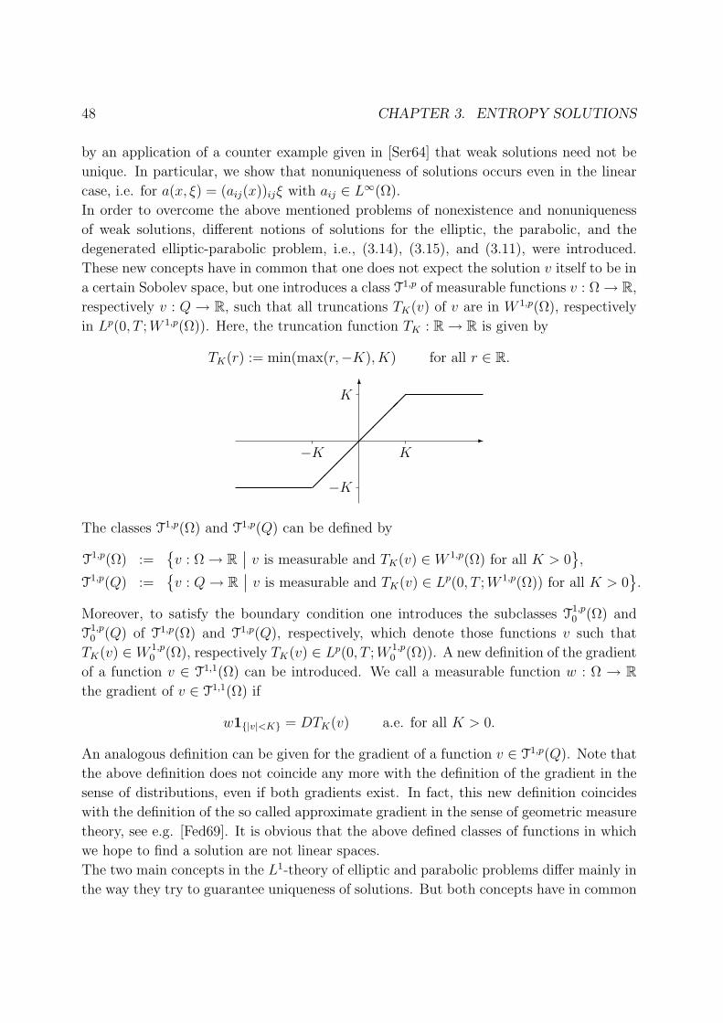
48 CHAPTER 3. ENTROPY SOLUTIONS
by an application of a counter example given in [Ser64] that weak solutions need not be
unique. In particular, we show that nonuniqueness of solutions occurs even in the linear
case, i.e. for a(x, ξ) = (aij(x))ijξ with aij ∈ L∞(Ω).
In order to overcome the above mentioned problems of nonexistence and nonuniqueness
of weak solutions, different notions of solutions for the elliptic, the parabolic, and the
degenerated elliptic-parabolic problem, i.e., (3.14), (3.15), and (3.11), were introduced.
These new concepts have in common that one does not expect the solution v itself to be in
a certain Sobolev space, but one introduces a class T1,p of measurable functions v : Ω → R,
respectively v : Q → R, such that all truncations TK(v) of v are in W 1,p(Ω), respectively
in Lp(0, T ;W 1,p(Ω)). Here, the truncation function TK : R → R is given by
TK(r) := min(max(r,−K), K) for all r ∈ R.
-
−K K
6
−K
K
The classes T1,p(Ω) and T1,p(Q) can be defined by
T1,p(Ω) :=v : Ω → R
∣∣ v is measurable and TK(v) ∈ W 1,p(Ω) for all K > 0,
T1,p(Q) :=v : Q→ R
∣∣ v is measurable and TK(v) ∈ Lp(0, T ;W 1,p(Ω)) for all K > 0.
Moreover, to satisfy the boundary condition one introduces the subclasses T1,p0 (Ω) and
T1,p0 (Q) of T1,p(Ω) and T1,p(Q), respectively, which denote those functions v such that
TK(v) ∈ W 1,p0 (Ω), respectively TK(v) ∈ Lp(0, T ;W 1,p
0 (Ω)). A new definition of the gradient
of a function v ∈ T1,1(Ω) can be introduced. We call a measurable function w : Ω → Rthe gradient of v ∈ T1,1(Ω) if
w1|v|<K = DTK(v) a.e. for all K > 0.
An analogous definition can be given for the gradient of a function v ∈ T1,p(Q). Note that
the above definition does not coincide any more with the definition of the gradient in the
sense of distributions, even if both gradients exist. In fact, this new definition coincides
with the definition of the so called approximate gradient in the sense of geometric measure
theory, see e.g. [Fed69]. It is obvious that the above defined classes of functions in which
we hope to find a solution are not linear spaces.
The two main concepts in the L1-theory of elliptic and parabolic problems differ mainly in
the way they try to guarantee uniqueness of solutions. But both concepts have in common
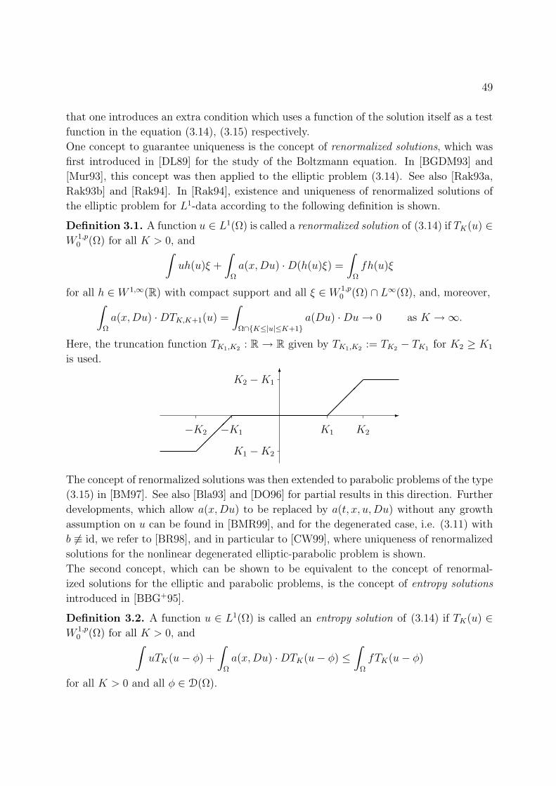
49
that one introduces an extra condition which uses a function of the solution itself as a test
function in the equation (3.14), (3.15) respectively.
One concept to guarantee uniqueness is the concept of renormalized solutions, which was
first introduced in [DL89] for the study of the Boltzmann equation. In [BGDM93] and
[Mur93], this concept was then applied to the elliptic problem (3.14). See also [Rak93a,
Rak93b] and [Rak94]. In [Rak94], existence and uniqueness of renormalized solutions of
the elliptic problem for L1-data according to the following definition is shown.
Definition 3.1. A function u ∈ L1(Ω) is called a renormalized solution of (3.14) if TK(u) ∈W 1,p
0 (Ω) for all K > 0, and∫uh(u)ξ +
∫Ω
a(x,Du) ·D(h(u)ξ) =
∫Ω
fh(u)ξ
for all h ∈ W 1,∞(R) with compact support and all ξ ∈ W 1,p0 (Ω) ∩ L∞(Ω), and, moreover,∫
Ω
a(x,Du) ·DTK,K+1(u) =
∫Ω∩K≤|u|≤K+1
a(Du) ·Du→ 0 as K →∞.
Here, the truncation function TK1,K2 : R → R given by TK1,K2 := TK2 − TK1 for K2 ≥ K1
is used.
-
−K2 −K1 K1 K2
6
K1 −K2
K2 −K1
The concept of renormalized solutions was then extended to parabolic problems of the type
(3.15) in [BM97]. See also [Bla93] and [DO96] for partial results in this direction. Further
developments, which allow a(x,Du) to be replaced by a(t, x, u,Du) without any growth
assumption on u can be found in [BMR99], and for the degenerated case, i.e. (3.11) with
b 6≡ id, we refer to [BR98], and in particular to [CW99], where uniqueness of renormalized
solutions for the nonlinear degenerated elliptic-parabolic problem is shown.
The second concept, which can be shown to be equivalent to the concept of renormal-
ized solutions for the elliptic and parabolic problems, is the concept of entropy solutions
introduced in [BBG+95].
Definition 3.2. A function u ∈ L1(Ω) is called an entropy solution of (3.14) if TK(u) ∈W 1,p
0 (Ω) for all K > 0, and∫uTK(u− φ) +
∫Ω
a(x,Du) ·DTK(u− φ) ≤∫
Ω
fTK(u− φ)
for all K > 0 and all φ ∈ D(Ω).
50 CHAPTER 3. ENTROPY SOLUTIONS
The main idea of the above definition is of course adapted from the theory of conservation
laws, where, in order to guarantee uniqueness, one introduces an entropy condition, see
[Kru70].
The concept of entropy solutions has also been extended to parabolic problems. In
[AMSdLT99], it is shown that for parabolic equations of the type (3.15) with strictly
monotone a, i.e., a satisfying (3.7), the concept of entropy solutions coincides with the
concept of mild solutions (see remark 1.4) of the nonlinear Cauchy problem
u′ + Au 3 f,u(0) = u0
for f ∈ L1(0, T ;L1(Ω)), u0 ∈ D(A) and A ⊂ L1(Ω) × L1(Ω) an m-completely accretive
operator in L1(Ω). Here, A can be constructed as follows, see also [AMSdLT97]. We first
define the operator A∞ ⊂ L1(Ω)× L1(Ω) by
(u,w) ∈ A∞ if and only if u ∈ W 1,p0 (Ω) ∩ L∞(Ω), w ∈ L1(Ω), and∫
Ω
a(x,Du) ·Dφ =
∫Ω
wφ
for all φ ∈ W 1,p0 (Ω) ∩ L∞(Ω).
(3.16)
The operator A∞ is completely accretive with D(A∞) = L1(Ω) and R(I+λA∞) ⊃ L∞(Ω)
for all λ > 0. Thus, we can define A := A∞ to be the graph-closure of A∞. Then, A is
an m-accretive operator in L1(Ω) with D(A) = L1(Ω), and for all f ∈ L1(0, T ;L1(Ω)) =
L1(Q), u0 ∈ L1(Ω), there exists a mild solution u ∈ C([0, T ];L1(Ω)) of the abstract
Cauchy problem (see remark 1.4) which is also the unique entropy solution of (3.15).
In order to characterize the operator A, we introduce the following notation. We call
a function S : R → R piecewise continuously differentiable, if there exist finitely many
points −∞ = t0 < t1 < · · · < tm−1 < tm = ∞ such that S∣∣(ti,ti−1)
∈ C1((ti, ti−1))
for i = 1, . . . ,m. Moreover, C1p(R) denotes the set of continuous piecewise continuously
differentiable functions on R. Letting
P :=S ∈ C1
p(R)∣∣∣ 0 ≤ S ′ ≤ 1, supp S ′ is compact and S(0) = 0
, (3.17)
the operator A can be represented as follows.
(u,w) ∈ A if and only if u,w ∈ L1(Ω), TK(u) ∈ W 1,p0 (Ω) for all K > 0, and∫
Ω
a(x,Du) ·DS(u− φ) ≤∫
Ω
wS(u− φ)
for all φ ∈ D(Ω), S ∈ P.
(3.18)
51
In section 3.2, we compare the two concepts in order to develop a solution theory for
L1-data of the history dependent degenerated elliptic-parabolic problem (3.1), (3.2). It
turns out that only the concept of entropy solutions can naturally be extended to this
case, since the derivative in time operator in (3.1) does not satisfy a Kato equality but
only a Kato inequality, see proposition 3.23 and corollary 3.24. Thus, we do not have an
integration by parts formula for
∂
∂t
(κ(u(t)− u0) +
∫ t
0
k(t− s)(u(s)− u0) ds
),
which is an essential tool in the theory of renormalized solutions of parabolic equations.
In section 3.3, we show uniqueness of entropy solutions of (3.1), (3.2) according to the
following definition.
Definition 3.3. Let (3.4)-(3.6), (3.8)-(3.10) and (3.3) be satisfied. A measurable func-
tion v : Q → R is called an entropy solution of (3.1), (3.2) if b(v) ∈ L1(Q), TK(v) ∈Lp(0, T ;W 1,p
0 (Ω)) for all K > 0, and
−∫
Q
ζt(t)[κ
∫ v(t)
v0
S(r − φ) db(r) +
∫ t
0
k1(t− s)
∫ v(s)
v0
S(r − φ) db(r) ds]
+
∫Q
ζ(t)[k2(0+)(b(v(t))− b(v0))
+
∫(0,t]
(b(v(t− s))− b(v0)) dk2(s)]S(v(t)− φ)
+
∫Q
ζ(t)a(x,Dv(t)) ·DS(v(t)− φ) ≤∫
Q
ζ(t)f(t)S(v(t)− φ)
for all φ ∈ D(Ω), ζ ∈ D([0, T )) with ζ ≥ 0, S ∈ P, where P is defined by (3.17), and
all nonnegative nonincreasing functions k1, k2 ∈ L1(0, T ), such that k = k1 + k2 and
k2(0+) <∞.
The above definition is adapted from the definition of entropy solutions for fractional
conservation laws as given in [CGL96, Definition 6]. A main tool in the proof of uniqueness
of entropy solutions of (3.1), (3.2) will be Kruzhkov’s method of doubling variables, see
[Kru70].
In section 3.4, we show existence of entropy solutions for the non-degenerated problem,
i.e., for (3.1), (3.2) with b ≡ id. In particular, we show that the generalized solution of the
abstract Volterra equation
d
dt
(κ(u(t)− u0) +
∫ t
0
k(t− s)(u(s)− u0) ds)
+ Au(t) 3 f(t) for t ∈ [0, T ),
52 CHAPTER 3. ENTROPY SOLUTIONS
with the operator A given by (3.18), is an entropy solution of (3.1), (3.2). To this end,
we approximate the problem (3.1), (3.2) by sequences of regular data u0,nn∈N, fnn∈N.
The main task in showing the existence of entropy solutions for (3.1), (3.2) is to obtain
convergence of the sequence of gradients Dunn∈N and of a(x,Dun)n∈N, where un is
the solution for the regular data u0,n, fn.
In the strictly monotone case we can show almost everywhere convergence of the sequence
Dun, and thus of a(x,Dun). In the general monotone case, only weak convergence of
DTK(un) in Lp(Q)N for all K > 0 can be shown by a priori estimates. Thus, one only
obtains weak convergence of a(x,DTK(un)) in Lp′(Q)N towards a(x,DTK(u)), where u
denotes the entropy solution, by a pseudo-monotonicity argument.
In the literature no result on the existence can be found for the degenerated case of
the elliptic-parabolic problem (3.11), i.e., with b continuous nondecreasing and possibly
constant on some interval. In particular, this problem is still open for the history dependent
problem (3.1), (3.2). Remarks on the existence of renormalized solutions in the degenerated
elliptic-parabolic case can be found in [BR98, BMR99] and [CW99]. We mention that the
method we use in the proof of existence for the non-degenerated problem fails in the
degenerated case, since there is no monotonicity in the time derivative operator any more,
as shown in example 3.25.
3.1 Nonexistence and nonuniqueness of weak solu-
tions
We assume that (3.4)-(3.6) and (3.8)-(3.10) are satisfied, and we consider the problem
(3.1), (3.2) for b ≡ id and L1-data u0 ∈ L1(Ω) and f ∈ L1(Q) = L1(0, T ;L1(Ω)). Defining
the operator A∞ ⊂ L1(Ω) × L1(Ω) by (3.16), it can be shown that A∞ is a completely
accretive operator in L1(Ω) with R(I + λA∞) ⊃ L∞(Ω) for all λ > 0. Moreover, its
closure A := A∞ is an m-completely accretive operator in L1(Ω); see for example [BW96,
Proposition 2.4] and [AMSdLT97].
As a consequence of the existence result of [CGL96] and [Gri85], we already know that
the abstract Volterra equation
d
dt
(κ(u(t)− u0) +
∫ t
0
k(t− s)(u(s)− u0) ds
)+ Av(t) 3 f(t) t ∈ [0, T ), (3.19)
admits a unique generalized solution u ∈ L1(0, T ;L1(Ω)) = L1(Q). In particular, we know
by the approximation result for generalized solutions that for any k ∈ L1loc([0,∞)) with
λ = k(0+) <∞ satisfying (3.8) there exists a unique strong solution u of
k(0+)u(t) + Au(t) 3 f(t) + k(0+)u0 −∫
(0,t]
(u(t− s)− u0) dk(s) t ∈ [0, T ). (3.20)
3.1. NONEXISTENCE AND NONUNIQUENESS OF WEAK SOLUTIONS 53
Thus, by the definition of A, u(t) ∈ L1(Ω) is almost everywhere for t ∈ (0, T ) in some
sense a solution of the initial value elliptic boundary value problem
k(0+)(u(t, x)− u0(x)) +
∫(0,t]
(u(t− s, x)− u0(x)) dk(s)
− div a(x,Du(t, x)) = f(t, x) in (0, T )× Ω
u = 0 on (0, T )× ∂Ω
u(0) = u0 in Ω.
(3.21)
As an example of the elliptic boundary value problem (3.21), consider
λu−∆pu = g in Ω,
u = 0 on ∂Ω.
Here, we have defined g ∈ L1(Ω) for t ∈ (0, T ) fixed by
g = f(t) + λu0 −∫
(0,t]
(u(t− s)− u0) dk(s).
Moreover, ∆p denotes the p-Laplacian given by ∆p = div a(Du) with a(ξ) = |ξ|p−2ξ. One
easily sees that the assumptions (3.4), (3.5) and (3.6) are satisfied for this choice of a.
When considering the problem (3.21), one naturally thinks of understanding the first
equation in (3.21) in the sense of distributions, i.e.,∫Ω
(d
dt
∫ t
0
k(t− s)(u(s, x)− u0) ds
)φ+
∫Ω
a(x,Du(t, x)) ·Dφ =
∫Ω
f(t, x)φ (3.22)
for all φ in the space of test function C∞c (Ω) and almost everywhere for t ∈ (0, T ). There-
fore we have to give a sense to the gradient Du of the solution u. Additionally, with regard
to the boundary condition (3.21), the largest space in which we want the solution u to be
is L1(0, T ;W 1,10 (Ω)). Thus, we consider the following definition of a weak solution.
Definition 3.4. A function u ∈ L1(0, T ;W 1,10 (Ω)) is called a weak solution of (3.21) for
f ∈ L1((0, T ) × Ω) and u0 ∈ L1(Ω), if a(x,Du) ∈ L1loc(Q), and u satisfies (3.22) for all
φ ∈ C∞c (Ω) and almost everywhere for t ∈ (0, T ).
Now, our intention is to show that there exists a function f ∈ L1((0, T ) × Ω) such that
the problem (3.21) does not admit a weak solution u ∈ L1(0, T ;W 1,10 (Ω)). Therefore, we
will construct a counterexample adapted from [BBG+95]. In this sense the definition 3.4
is not sufficient for the problem of existence. The main idea of showing the nonexistence
of solutions will be the following nonembedding property.
Lemma 3.5. Let Ω be an open subset of RN with N ≥ 2 then W−1,∞(Ω) ∩W 1,N0 (Ω) 6⊂
L∞(Ω).
54 CHAPTER 3. ENTROPY SOLUTIONS
Proof. We construct a function which is an element of W−1,∞(Ω)∩W 1,N0 (Ω) but which is
not essentially bounded. Let x ∈ Ω and R > 0 such that the open ball BR(x) with radius
R centered at x is contained in Ω. For all x ∈ BR(x)\x, we define
u(x) := ln
(ln
(R exp(1)
ρ
)), with ρ := |x− x| =
√√√√ N∑i=1
(xi − xi)2,
and u(x) = 0 for all x ∈ (Ω\BR(x)) ∪ x. Then, by limx→x u(x) = ∞, it is obvious that
u 6∈ L∞(Ω). We now show that u ∈ W 1,N0 (Ω). By the simple estimate∫
Ω
|u|N dx =
∫BR(x)
ln
(ln
(R exp(1)
ρ
))N
dx
= CN
∫ R
0
ln
(ln
(R exp(1)
r
))N
rN−1 dr
= CN
∫ ∞
1
ln(s)NRN exp (N(1− s)) ds
≤ CNRN
∫ ∞
1
sN exp (N(1− s)) ds <∞,
we obtain u ∈ LN(Ω). The distributional derivative of u is given by
∂u
∂xi
= − 1
ln(
R exp(1)ρ
) · ρ
R exp(1)· R exp(1)
ρ2· ∂ρ∂xi
,
almost everywhere for x ∈ BR(x), and ∂u∂xi
= 0 almost everywhere for x ∈ Ω\BR(x). Here
we have ∂ρ∂xi
= xi−xi
ρ, and thus | ∂ρ
∂xi| ≤ 1 for i = 1, ..., N . This implies∫
Ω
| ∂u∂xi
|N dx ≤∫
BR(x)
ln
(R exp(1)
ρ
)−N1
ρNdx
= C
∫ R
0
ln
(R exp(1)
r
)−N
rN−N−1 dr
= C
∫ ∞
1
s−N ds <∞.
Thus, we conclude u ∈ W 1,N(Ω). Moreover, by limρ→R u(x) = 0 and u(x) = 0 almost
everywhere for x ∈ Ω\BR(x), we obtain u ∈ W 1,N0 (Ω).
It remains to show that u ∈ W−1,∞(Ω). To this end, we define the functions Ui for
i = 1, ..., N by
Ui(x) := −xi − xi
Nln
(ln
(R exp(1)
ρ
)), with ρ := |x− x| =
√√√√ N∑i=1
(xi − xi)2,
3.1. NONEXISTENCE AND NONUNIQUENESS OF WEAK SOLUTIONS 55
for x ∈ BR(x) \ x, and Ui(x) := 0 for all x ∈ (Ω\BR(x)) ∪ x. Defining
U0(x) :=1
N· 1
ln(
R exp(1)ρ
)for x ∈ BR(x) \ x, and U0(x) := 0 for all x ∈ (Ω\BR(x0)) ∪ x, we easily see that
Ui ∈ L∞(Ω) for i = 0, ..., N . Additionally, we obtain for all v ∈ W 1,10 (Ω)∫
Ω
uv =
∫BR(x)
[ 1
N
1
ln(
R exp(1)ρ
) − N∑i=1
(xi − xi)2
ρ2N
1
ln(
R exp(1)ρ
)+ ln
(ln
(R exp(1)
ρ
))]v
=
∫Ω
U0v +N∑
i=1
∫Ω
Ui∂v
∂xi
.
Here, we used the fact that limρ→R Ui(x) = 0 for i = 1, ..., N . This implies u ∈ W−1,∞(Ω),
which completes the proof.
In order to show the nonexistence of weak solutions for (3.21) for certain f ∈ L1((0, T )×Ω)
and u0 ∈ L1(Ω), we need to show the following duality.
Lemma 3.6.(W 1,1
0 (Ω) +W−1,q′(Ω))′
= W−1,∞∩W 1,q0 holds for 1 < q <∞ with q′ = q
q−1.
We first note that a couple (X1, X2) of Banach spaces is called compatible if Xi is contin-
uously embedded in a Hausdorff topological vector space X for i = 1, 2. For a compatible
couple of Banach spaces (X1, X2) the spaces X1+X2 and X1∩X2 are again Banach spaces,
endowed with the norms
‖x‖X1+X2 := inf‖x1‖X1 + ‖x2‖X2
∣∣∣ x = x1 + x2 with x1 ∈ X1, x2 ∈ X2
,
respectively
‖x‖X1∩X2 := max ‖x‖X1 , ‖x‖X2 .
To prove lemma 3.6, we will make use of the following abstract result on the dual space
of a sum of Banach spaces, see e.g. [BS88, Exercise 3.2]
Proposition 3.7. Let (X1, X2) be a compatible couple of Banach spaces, and let X1 ∩X2
be dense in Xi for i = 1, 2. Then (X1 +X2)′ = X ′
1 ∩X ′2.
Proof of lemma 3.6. By proposition 3.7, it is sufficient to show that W 1,10 (Ω) ∩W−1,q′(Ω)
is dense in W 1,10 (Ω) and in W−1,q′(Ω).
56 CHAPTER 3. ENTROPY SOLUTIONS
Therefore, we first note that C∞c (Ω) ⊂ W 1,1
0 (Ω)∩W−1,q′(Ω). And, by definition ofW 1,10 (Ω),
the space C∞c (Ω) is dense in W 1,1
0 (Ω).
Take an element F ∈ W−1,q′(Ω). Then there exist fi ∈ Lq′(Ω) for i = 0, ..., N such that
for all v ∈ W 1,q0 (Ω)
〈F, v〉 =
∫Ω
f0v +N∑
i=1
∫Ω
fi∂v
∂xi
.
Choosing approximating sequences (φ(i)n )n∈N ⊂ C∞
c (Ω) for i = 0, ..., N with φ(i)n → fi in
Lq′(Ω) as n→∞, we can define
〈Fn, v〉 :=
∫Ω
φ(0)n v +
N∑i=1
∫Ω
φ(i)n
∂v
∂xi
for all v ∈ W 1,q(Ω)0 . Then, obviously,
|〈F − Fn, v〉| ≤ max‖fi − φ(i)
n ‖Lq′ (Ω)
∣∣∣i = 0, ..., N‖v‖W 1,q
0 (Ω),
and thus Fn → F in W−1,q′(Ω) as n→∞.
Proposition 3.8. Let Ω be a bounded domain in RN , and let 1 < p ≤ 2− 1N
. Then there
exists a function f ∈ L1((0, T ) × Ω) such that the problem (3.21) with u0 ≡ 0 does not
admit a weak solution u ∈ L1(0, T ;W 1,10 (Ω)).
Proof. First assume that for f ∈ L1((0, T ) × Ω) and u0 ≡ 0 there exists a weak solution
u of (3.21), i.e. u ∈ L1(0, T ;W 1,10 (Ω)) satisfying (3.22). We show by using the growth
bound (3.6) that a(Du) ∈ Lq′((0, T ) × Ω), with q := 12−p
and q′ := qq−1
= 1p−1
. The fact
that q′ = 1p−1
< pp−1
= p′, i.e., that Lp′((0, T )× Ω) ⊂ Lq′((0, T )× Ω) holds, yields(∫ T
0
∫Ω
|a(Du)|q′) 1
q′
≤ Λ
(T p−1‖j‖Lq′ (Ω) +
(∫ T
0
∫Ω
|Du|(p−1)q′)p−1
)≤ Λ
(C‖j‖Lp′ (Ω) + ‖u‖p−1
L1(0,T ;W 1,1(Ω))
).
Thus, we have shown that diva(Du) ∈ Lq′(0, T ;W−1,q′(Ω)). By the definition of weak
solutions this implies that f ∈ L1(0, T ;W 1,10 (Ω)) + Lq′(0, T ;W−1,q′(Ω)).
In the second step, assume that for each f ∈ L1((0, T ) × Ω) there exists a weak solution
u ∈ L1(0, T ;W 1,10 (Ω)) of the elliptic boundary value problem (3.21) with u0 ≡ 0. This
implies by our first conclusion that
L1((0, T )× Ω) ⊂ L1(0, T ;W 1,10 (Ω)) + Lq′(0, T ;W−1,q′(Ω)).
Hence,
L1(Ω) ⊂ W 1,10 (Ω) +W−1,q′(Ω).
3.1. NONEXISTENCE AND NONUNIQUENESS OF WEAK SOLUTIONS 57
By duality and Lemma 3.6 we obtain
W−1,∞(Ω) ∩W 1,q0 (Ω) ⊂ L∞(Ω).
But the assumption q = 12−p
≤ N implies
W−1,∞(Ω) ∩W 1,N0 (Ω) ⊂ W−1,∞(Ω) ∩W 1,q
0 (Ω) ⊂ L∞(Ω).
This is a contradiction to the nonembedding shown in Lemma 3.5. Thus, there exists a
function f ∈ L1((0, T ) × Ω) such that the problem (3.21) with u0 ≡ 0 does not admit a
weak solution.
As a consequence of the above result, we can not expect the generalized solution u of (3.20)
to be a weak solution of the elliptic boundary value problem (3.21) almost everywhere for
t ∈ (0, T ), even though u is a strong solution of the abstract Volterra equation (3.20).
Moreover, if κ, k satisfy (3.9), we can show nonexistence of weak solutions of (3.1) with
b ≡ 0, by using the same methods as above.
Corollary 3.9. Let Ω be a bounded domain in RN , and let 1 < p ≤ 2− 1N
. Let b ≡ 0 and
let κ, k be arbitrary. Then there exists f ∈ L1(Q) such that (3.1) does not admit a weak
solution.
We further show that weak solutions of Volterra equations are in general not unique. To
this end, we will adapt the example given in [Ser64], see also [Pri95] and [Pri97].
Example 3.10. We consider the linear elliptic problem∑i,j
∂
∂xi
(aij
∂u
∂xj
)= 0 (3.23)
on the open unit ball BR2 of R2. Here, we define the coefficients aij ∈ L∞(BR2) for
r :=√x2
1 + x22 by
aij := δij + (a− 1)xixj
r2. (3.24)
Then, it is easy to show that the matrix (aij)ij satisfies the coercivity assumption∑i,j
aijξiξj ≥ σ|ξ|2 for all ξ = (ξi)i ∈ R2 with some σ > 0 (3.25)
for all a > 0. Note that for a ≥ 1 the coercivity assumption (3.25) is trivially satisfied
with σ = 1 and that for 0 < a < 1 one can obtain (3.25) for σ = a > 0. We now define
the notion of weak solutions for (3.23).
58 CHAPTER 3. ENTROPY SOLUTIONS
Definition 3.11. A function u ∈ W 1,1(BR2) is called a weak solution of (3.21) if∫BR2
aij∂u
∂xj
∂ϕ
∂xi
dx = 0 for all ϕ ∈ D(BR2) = C∞c (BR2).
Let 0 < ε < 1, and choose a :=1
ε2. Defining u : BR2 → R by
u(x) := x1r−(1+ε), (3.26)
it is easy to see that for some constants ci > 0 with i = 0, 1, 2∫BR2
|u|2 dx = c0
∫ 1
0
r1−2ε dr, and
∫BR2
∣∣∣∣ ∂u∂xi
∣∣∣∣β dx = ci
∫ 1
0
r1−β(1+ε) dr for i = 1, 2.
Thus, u ∈ L2(BR2) ∩W 1,β(B2R) for all β < 2
1+ε< 2. But u 6∈ H1(BR2). Moreover, since u
is C∞ for r > 0, it is easy to show that u ∈ H1/2(S1), where S1 = ∂BR2 , see also [Pri95].
By simple calculation, one obtains∫ ∑i,j
aij∂u
∂xj
∂ϕ
∂xi
dx = lim%→0+
∫r>%
∑i,j
aij∂u
∂xj
∂ϕ
∂xi
dx
= − lim%→0+
∫r=ρ
ϕ∑i,j
aij∂u
∂xj
xi
rds
=1
εlim
%→0+%−(2+ε)
∫r=ρ
x1ϕ ds
= 0
for all ϕ ∈ D(BR2), since for all ϕ ∈ D(BR2) we have
%−(2+ε)
∣∣∣∣∫r=ρ
x1ϕ ds
∣∣∣∣ ≤ %1−ε
∥∥∥∥ ∂ϕ∂x1
∥∥∥∥∞
∫ 2π
0
cos2 θ dθ → 0 as %→ 0 + .
Thus, we have shown that u is a weak solution of (3.23). Due to u ∈ H1/2(S1), there exists
a unique variational solution v ∈ H1(BR2) of the linear elliptic boundary value problem∑i,j
∂
∂xi
(aij
∂v
∂xj
)= 0 in BR2
v = u on S1.
Defining w0 := u − v, we conclude that the elliptic boundary value problem given by
(3.23) with Dirichlet boundary condition, i.e., u = 0 on S1, admits a weak solution w0 ∈L2(BR2) ∩ W 1,β(BR2) for all β < 2
1+εsuch that w0 6∈ H1
0 (BR2), which implies that w0
is different from the variational solution of the same problem. Hence, weak solutions of
elliptic boundary value problems are in general not unique.
3.1. NONEXISTENCE AND NONUNIQUENESS OF WEAK SOLUTIONS 59
We are now going to show that this nonuniqueness carries over to Volterra equations.
Example 3.12. We consider for w0 and aij defined as above and for 0 < γ < 1 the
parabolic problem
∂
∂t
∫ t
0
s−γ
Γ(1− γ)(w(t− s, x)− w0(x)) ds
−∑i,j
∂
∂xi
(aij
∂w
∂xj
(t, x)
)= 0 in (0, T )×BR2 ,
w(0, ·) = w0 in BR2 ,
w(t, x) = 0 on (0, T )× S1.
(3.27)
Using the following definition of weak solutions for (3.27), it is obvious that the function
w : [0, T ) × BR2 → R defined by w(t, x) := w0(x) for all (t, x) ∈ [0, T ) × BR2 is a weak
solution of the above problem.
Definition 3.13. A function w ∈ L1(0, T ;W 1,10 (BR2)) is called a weak solution of (3.27)
if for all ϕ ∈ D([0, T )×BR2)
−∫
(0,T )×BR2
∫ t
0
s−γ
Γ(1− γ)(w(t− s, x)− w0(x)) ds
∂
∂tϕ(t, x) dx dt
+
∫(0,T )×BR2
∑i,j
aij∂w
∂xj
(t, x)∂ϕ
∂xi
(t, x) dx dt = 0.
If we now define the operator A : D(A) → L2(BR2) by
Au :=∑i,j
∂
∂xi
(aij
∂v
∂xj
)for all u ∈ D(A) with
D(A) :=v ∈ H1
0 (BR2)∣∣∣ ∑
i,j
∂
∂xi
(aij
∂v
∂xj
)∈ L2(BR2)
,
then it is clear that A is a densely defined linear operator in L2(BR2) generating a C0-
semigroup. Moreover, one can show, by the same methods as used in [Paz83, Theorem
7.2.7], that A generates an analytic semigroup on L2(BR2). Concerning the analyticity of
the semigroup generated by A, we also refer to [DL84, Exemple III.17B.3.2]. Using [Pru93,
Corollary 1.2.4], we conclude that the linear Volterra equation
u(t) = w0 +
∫ t
0
(t− s)γ−1
Γ(γ)Au(s) ds (3.28)
admits an analytic resolvent S(t)t≥0. Applying [Pru93, Theorem 1.2.2] to v(·) := S(·)w0,
we conclude that v ∈ C([0, T );L2(BR2)) with v(t) ∈ H10 (BR2)) for all t ∈ (0, T ). Since, by

60 CHAPTER 3. ENTROPY SOLUTIONS
the definition of A, v is also a weak solution of (3.27) and v 6= w ≡ w0 6∈ H10 (BR2), we
have shown that weak solutions of (3.27) are not unique. Therefore, the concept of weak
solutions for Volterra equations is not sufficient in order to guarantee uniqueness.
We remark that the same results as above can be obtained in more than two space di-
mensions. This can easily be seen considering the function u(x) := x1(x21 + x2
2)−(1+ε)/2 on
BRN , and defining aij = δij for the additional coefficients of the matrix (aij)ij.
3.2 A Kato inequality
This section deals with Kato inequalities for operators corresponding to the derivative in
time in the Volterra equation (3.1). The min results are stated in proposition 3.23 and
corollary 3.24. Thus, for T > 0, we consider operators of the type
B : D(B) ⊂ L1(0, T ) → L1(0, T )
B(u)(t) :=d
dt
(κu(t) +
∫ t
0
k(t− s)u(s) ds
),
with
D(B) :=u ∈ L1(0, T )
∣∣∣ t 7→ κu(t) +
∫ t
0
k(t− s)u(s) ds ∈ W 1,10 (0, T )
,
(3.29)
with κ, k satisfying (3.8). Here, we define W 1,10 (0, T ) := u ∈ W 1,1(0, T ) | u(0) = 0. The
results obtained in this section are essential for the study of existence and uniqueness of
entropy solutions of the history dependent problem (3.1), (3.2).
Before turning to Kato inequalities, we remark that a Kato inequality will replace the
integration by parts formula which was used in the L1-theory for degenerated elliptic-
parabolic equations of the type
b(v)t = div a(x,Du) + f in Q := (0, T )× Ω,
v = 0 on (0, T )× ∂Ω,
b(v)(0, ·) = b(v0) in Ω.(3.30)
Here, the same assumptions as for (3.1) apply, i.e., we assume (3.4)-(3.6), (3.8)-(3.10)
and (3.3). Using the definition of the set P given in (3.17), one can show the following
integration by parts formula.
Lemma 3.14. Let b : R → R be continuous and nondecreasing with b(0) = 0, v ∈Lp(0, T ;W 1,p
0 (Ω)) with b(v) ∈ L1(Q), b(v)t ∈ Lp′(0, T ;W−1,p′(Ω)) +L1(Q) and b(v)(0, ·) =
b(v0), where v0 : Ω → R is measurable with b(v0) ∈ L1(Ω). Then
−∫ T
0
〈b(v)t, ξS(v − φ)〉 =
∫Q
ξt
∫ v
v0
S(r − φ) db(r) dx dt
3.2. A KATO INEQUALITY 61
for all ξ ∈ D([0, T )), S ∈ P and all φ ∈ D(Ω). Moreover,
−∫ T
0
〈b(v)t, ξh(v)〉 =
∫Q
ξt
∫ v
v0
h(r) db(r) dx dt
for all h ∈ W 1,∞(R), ξ ∈ W 1,∞(Q) with ξ(T ) = 0 and h(v)ξ ∈ Lp(0, T ;W 1,p0 (Ω)). Here,
〈·, ·〉 denotes the duality pairing between W−1,p′(Ω) + L1(Ω) and W 1,p0 (Ω) ∩ L∞(Q).
The proof of the above lemma can be done by using exactly the same methods as in
[CW99, Lemma 1.4 and Lemma 4.3], see also [AL83, Lemma 1.5] and [Ott96].
Since this integration by parts formula holds, there are two concepts of solutions of (3.30)
in order to guarantee uniqueness. One concept is the concept of entropy solutions.
Definition 3.15. A measurable function v : Q→ R is called an entropy solution of (3.30)
if b(v) ∈ L1(Q), TK(v) ∈ Lp(0, T ;W 1,p0 (Ω)) for all K > 0, and for all φ ∈ D(Ω), S ∈ P,
ξ ∈ D([0, T )) with ξ ≥ 0
−∫
Q
ξt
∫ v
v0
S(r − φ) db(r) +
∫Q
ξ a(x,Dv) ·DS(v − φ) ≤∫
Q
ξfS(v − φ).
The second concept is the concept of renormalized solutions.
Definition 3.16. A measurable function v : Q → R is called a renormalized solution
of (3.30), if b(v) ∈ L1(Q), TK(v) ∈ Lp(0, T ;W 1,p0 (Ω)) for all K > 0, for all h ∈ C1
c (R),
ξ ∈ D([0, T )× Ω)
−∫
Q
ξt
∫ v
v0
h(r) db(r) +
∫Q
a(x,Dv) ·D(ξh(v)) =
∫Q
ξfh(v), (3.31)
and ∫Q
a(x,Dv) ·DTK,K+1(v) =
∫Q∩K≤|v|≤K+1
a(x,Dv) ·Dv → 0 as K →∞.
Whereas the concept of entropy solutions is only based on an inequality, the concept of
renormalized solutions is based on the equality (3.31). Thus, in order to show that weak
solutions v ∈ Lp(0, T ;W 1,p0 (Ω)) satisfying b(v) ∈ L1(Q) are as well renormalized solutions,
one has to apply an integration by parts formula, as done in [CW99, Proposition 1.3].
Note that for (3.30) the two concepts coincide, i.e. a measurable function v : Q→ R is an
entropy solution of (3.30) if and only if it is a renormalized solution.
The main problem that occurs when replacing the operator ∂/∂t in (3.30) by the nonlocal
operator B defined by (3.29) is that we can not expect the integration by parts formula
to hold in this case. Indeed, we have the following result.
62 CHAPTER 3. ENTROPY SOLUTIONS
Example 3.17. Take b ≡ id, κ = 0, k(t) := t−γ/Γ(1− γ) for 0 < γ < 1, and an arbitrary
bounded domain Ω ⊂ RN . We define v0 :≡ 0, and v(t, x) := tφ(x) for all (t, x) ∈ Q,
where φ ∈ D(Ω). Since v is bounded, we may take p ∈ C∞(R) with 0 ≤ p′ ≤ 1 such that
p(v) ≡ v. Then, by simple calculation, we see that for certain choices of φ ∈ D(Ω) and
ξ ∈ D([0, T )) with φ, ξ ≥ 0∫Q
ξ(t)
(∂
∂t
∫ t
0
k(t− s)(v(s)− v0) ds
)p(v(t)) dx dt
=
∫Ω
φ2 dx
∫ T
0
ξ(t)t2−γ
Γ(2− γ)dt
>
∫Ω
φ2 dx
∫ T
0
ξ(t)t2−γ
Γ(3− γ)dt
= −∫
Ω
φ2 dx
∫ T
0
ξt(t)t3−γ
(3− γ)Γ(3− γ)dt
= −∫
Q
ξt(t)
∫ t
0
k(t− s)
∫ v(s)
v0
p(r) dr ds dx dt.
As a consequence, one can not extend the concept of renormalized solutions to the problem
given by the Volterra equation (3.1) in a straightforward way, since one can not even expect
weak solutions v ∈ Lp(0, T ;W 1,p0 (Ω)) with b(v) ∈ L1(Q) to satisfy (3.31) with∫
Q
ξt
∫ v
v0
h(r) db(r) dx dt replaced by
∫Q
ξt
∫ t
0
k(t− s)
∫ v(s)
v0
h(r) db(r) dx dt.
But the concept of entropy solutions might still be applicable if we can show an appropriate
inequality. This will be done in proposition 3.23 and corollary 3.24.
To understand more clearly why we do not have an integration by parts formula for the
operator B defined by (3.29), and what we can expect to hold otherwise, we now consider
the above problem in an abstract setting.
It is well known that the operator − ddt
generates the translation semigroup (T (τ))τ≥0 on
C0(R). Here, C0(R) denotes the space of continuous functions converging to 0 for |t| → ∞.
The translation semigroup given by T (τ)f = f(· − τ) for all τ ≥ 0 and all f ∈ C0(R) is
strongly continuous on C0(R). In order to characterize semigroups and their infinitesimal
generators we introduce the following notions.
Definition 3.18. Let T : V → V be a bounded linear operator on V , where V = C0(R)
or V = Lp(R) for some 1 ≤ p <∞.
(i) For V = C0(R), the operator T is called a homomorphism if T is a homomorphism
of the algebra C0(R), i.e. T is linear and T (fg) = (Tf)(Tg) for all f, g ∈ C0(R).
3.2. A KATO INEQUALITY 63
(ii) T is called submarkovian if 0 ≤ Tf ≤ 1 holds almost everywhere in R for all f ∈ Vwith 0 ≤ f ≤ 1 a.e. in R.
(iii) T is called positive if 0 ≤ Tf holds almost everywhere in R for all f ∈ V with 0 ≤ f
a.e. in R.
(iv) T is called translation invariant if T (f(· − s)) = (Tf)(· − s) for all s ∈ R.
It is obvious that the translation semigroup (T (τ))τ≥0 is a semigroup of homomorphisms,
i.e. T (τ) is a homomorphism for all τ ≥ 0. We define
J0 =j : R → (−∞,∞]
∣∣∣ j is convex and lower semicontinuous with j(0) = 0. (3.32)
For j ∈ J0, let D(j) = t ∈ R | j(t) < ∞. Then, according to [AB92, Theoreme 13],
we can fully characterize infinitesimal generators of strongly continuous semigroups of
homomorphisms.
Proposition 3.19. Let −A be the infinitesimal generator of a strongly continuous semi-
group (S(τ))τ≥0 on C0(R). Then the following assertions are equivalent:
(i) (S(τ))τ≥0 is a semigroup of homomorphisms.
(ii) fg ∈ D(A) and A(fg) = fAg + gAf for all f, g ∈ D(A).
(iii) For all j ∈ J0, f ∈ D(A) with f(R) ⊂ D(j), µ ∈ D(A′), w ∈ L1(R, |µ|) with
w(t) ∈ ∂j(f(t)) |µ|-a.e. for t ∈ R, the following Kato equality is satisfied
〈A′µ, j f〉 =
∫RwAf dµ. (3.33)
Here, A′ denotes the adjoint of the operator A.
By the above result it is clear that we can only expect an integration by parts formula
to hold if the corresponding operator generates a semigroup of homomorphisms, which is
equivalent to a product rule.
As we will see, in case of Volterra equations the operator given by the derivative in time
does not generate a semigroup of homomorphisms on C0(R) in general, but still generates a
strongly continuous semigroup of translation invariant submarkovian operators on C0(R),
respectively on Lp(R) for 1 ≤ p <∞.
Assume that the pair (κ, k) satisfies (3.8). Then, by [CP90, Theorem 1.6], there exists a
unique Bernstein function ϕ : (0,∞) → R such that
ϕ(z) = z(κ+ k(z)) for all z > 0,
64 CHAPTER 3. ENTROPY SOLUTIONS
where k denotes the Laplace-Transform of k. Moreover, there is a one-to-one correspon-
dence between the class of Bernstein functions and pairs (κ, k) satisfying (3.8).
According to [BF75, Proposition 9.2], for a function ϕ : (0,∞) → R to be a Bernstein
function is equivalent to the condition
ϕ ≥ 0 and (0,∞) 3 z 7→ exp(−τϕ(z)) is completely monotone for all τ > 0.
Applying Bernstein’s theorem, we conclude that there exists a family (ητ )τ>0 of nonnega-
tive Radon measures on R+ = [0,∞) such that
ητ (z) =
∫R+
e−zt dητ (t) = exp(−τϕ(z)) for all z > 0, τ > 0. (3.34)
In order to characterize the family (ητ )τ>0, we introduce the following notion.
Definition 3.20. A family (µτ )τ>0 of nonnegative bounded Radon measures on R is called
a convolution semigroup if
(i) µτ (R) ≤ 1 for all τ > 0,
(ii) µτ ∗ µσ = µτ+σ for all τ, σ > 0,
(iii) µτ ∗ δ0 in (Cc(R))′ as τ → 0+.
Here, µ ∗ ν denotes the convolution of measures, and δt denotes the Dirac measure at the
point t ∈ R.
Extending the measure ητ for all τ > 0 by ητ (A) = ητ (A∩[0,∞)) for all measurable subsets
A ⊂ R, one can show that the family (ητ )τ>0 is a convolution semigroup, in particular the
convolution ητ ∗ ησ is well defined, since all measures are supported on R+. Moreover, by
[BF75, Theorem 9.18], there is a one-to-one correspondence between the class of Bernstein
functions and the convolution semigroups supported on R+, where the correspondence is
given by (3.34).
Moreover, we may define for V = C0(R) and for V = Lp(R) with 1 ≤ p <∞
S(0)f = f and S(τ)f = f ∗ ητ for all τ > 0, f ∈ V. (3.35)
Then it is well known that the family (S(τ))τ≥0 is a strongly continuous semigroup on
C0(R), respectively on Lp(R). Moreover, the operators S(τ) are submarkovian for all
τ ≥ 0, since ητ is a nonnegative measure on R satisfying ητ (R) ≤ 1 for all τ > 0. Then,
according to [AB92, Theoreme 4], one can still show a Kato inequality.
3.2. A KATO INEQUALITY 65
Proposition 3.21. (i) Let −A be the infinitesimal generator of a strongly continuous
semigroup (S(τ))τ≥0 of submarkovian operators on Lp(R) for 1 ≤ p <∞. Then∫R(A′g)(j f) ≤
∫Rwg(Af)
for all j ∈ J0, 0 ≤ g ∈ D(A′), f ∈ D(A) with f(t) ∈ D(j) a.e. for t ∈ R such that
j f ∈ Lp(R), w ∈ L∞(R) with w(t) ∈ ∂j(f(t)) a.e. for t ∈ R. Here, A′ denotes the
adjoint of A.
(ii) Let −A be the infinitesimal generator of a strongly continuous semigroup (S(τ))τ≥0 of
submarkovian operators on C0(R). Then
〈A′µ, j f〉 ≤∫
Rw(Af) dµ
for all j ∈ J0, 0 ≤ µ ∈ D(A′), f ∈ D(A) with f(t) ∈ D(j) for all t ∈ R, w ∈ L1(R) with
w(t) ∈ ∂j(f(t)) |µ|-a.e. for t ∈ R.
For the sake of completeness, we give the proof in case of a submarkovian semigroup on
Lp(R) for 1 ≤ p <∞.
Proof. Let j, g, f, w be chosen as stated above. Then, by w ∈ ∂j(f) a.e., we conclude for
all τ ≥ 0
j S(τ)f ≥ j f + w(S(τ)f − f) a.e. in R.
Since S(τ) is submarkovian, we obtain by applying Jensen’s inequality S(τ)(j f) ≥j S(τ)f almost everywhere in R for all τ ≥ 0. This implies
−∫
R
S ′(τ)g − g
τj(f) = −
∫RgS(τ)j(f)− j(f)
τ≤ −
∫Rgj
(S(τ)f − f
τ
)for all τ ≥ 0. Noting that j is continuous onD(j), and that A′ is the infinitesimal generator
of the dual semigroup (S ′(τ))τ≥0 in X ′ endowed with the weak∗ topology, we can take the
limit for τ → 0+ in the above inequality and obtain the assertion.
Note that, according to [BF75, Theorem 12.7], there is a one-to-one correspondence be-
tween convolution semigroups on R and strongly continuous contraction semigroups of
translation invariant submarkovian operators on Lp(R) for 1 ≤ p <∞.
Having constructed a strongly continuous semigroup (S(τ))τ≥0 on Lp(R) for given κ, k
satisfying (3.8), and already knowing that the infinitesimal generator−Bp of the semigroup
satisfies a Kato inequality, we refer to [CP90, Theorem 4.1] for the actual calculation of
the infinitesimal generator.
66 CHAPTER 3. ENTROPY SOLUTIONS
Proposition 3.22. Let κ, k satisfy (4.2), choose k1 ∈ L1(R+), k2 ∈ BV (R+) satisfying
(4.2) such that k = k1 + k2, and define for 1 ≤ p <∞
D(Bp) :=f ∈ Lp(R)
∣∣∣ κf + k1 ∗ f ∈ W 1,p(R), and for all f ∈ D(Bp)
Bpf :=d
dt
(κf(t) +
∫ ∞
0
k1(t− s)f(s) ds
)+ k2(0+)f(t) +
∫(0,∞)
f(t− s) dk2(s).
Then −Bp is the infinitesimal generator of the semigroup (S(τ))τ≥0 defined by (3.35).
Returning to our original problem (3.1) on Q = (0, T )×Ω and omitting the calculation of
the adjoint of the time derivative operator, we can still show the following Kato inequality
which can be considered as a generalization of [GLS90, Exercise 20.6.30] and will serve as
a replacement of the integration by parts formula.
Proposition 3.23. Let κ, k satisfy (3.8), b : R → R be continuous and nondecreasing,
v : Q→ R and v0 : Ω → R be measurable such that b(v) ∈ BV (0, T ;L1(Ω)), b(v0) ∈ L1(Ω)
with b(v)(0+, ·) = b(v0) and(κ((b(v))−b(v0))+k∗(b(v)−b(v0))
)∈ W 1,1(0, T ;L1(Ω)). Then
−∫
Q
ξt(t)(κ
∫ v(t)
v0
S(r − φ) db(r) +
∫ t
0
k(t− s)
∫ v(s)
v0
S(r − φ) db(r) ds)
≤∫
Q
∂
∂t
(κ(b(v(t))− b(v0)) +
∫ t
0
k(t− s)(b(v(s))− b(v0)) ds
)S(v(t)− φ)ξ(t)
(3.36)
for all S ∈ P, φ ∈ D(Ω), ξ ∈ D([0, T )) with ξ ≥ 0. Moreover,
κ
∫Ω
∫ v(T )
v0
S(r − φ) db(r) +
∫ T
0
∫Ω
k(T − s)
∫ v(s)
v0
S(r − φ) db(r) ds
≤∫ T
0
∫Ω
∂
∂t
(κ(b(v(t))− b(v0)) +
∫ t
0
k(t− s)(b(v(s))− b(v0)) ds
)S(v(t)− φ)
(3.37)
for all S ∈ P, φ ∈ D(Ω).
Proof. As by assumption u := b(v) ∈ BV (0, T ;L1(Ω)) and u0 := b(v0) ∈ L1(Ω), we
conclude by applying [Gri85, Lemma 3.4] that k ∗ (u − u0) ∈ W 1,1(0, T ;L1(Ω)). Thus,
κu ∈ W 1,1(0, T ;L1(Ω)).
For a maximal monotone graph β in R×R with 0 ∈ β(0), we use the notation β0 for the
minimal section of β, given by β0(t) := sign0(s) mins∈β(t) |s| for all t ∈ R with β(t) 6= ∅.Letting S ∈ P and defining jx : R → (−∞,∞] by
jx(r) :=
∫ r
0
S(· − φ(x)) (b−1)0(s) ds for r ∈ R(b),
and
jx(r) := ∞ for r 6∈ R(b)
3.2. A KATO INEQUALITY 67
for all x ∈ Ω, it is clear that jx ∈ J0 and that w := S(v−φ) ∈ ∂jx(b(v)) almost everywhere
in Q, where ∂jx denotes the subdifferential of jx. Thus, we conclude for all r, r ∈ R∫ r
r
S(s− φ(x)) db(s) = jx(b(r))− jx(b(r)) ≥(b(r)− b(r)
)S(r − φ(x)).
(1) Choosing φ ∈ D(Ω), ξ ∈ D([0, T )) arbitrary with ξ ≥ 0, and defining v(t, ·) := v0 for
t < 0, it is clear that ζ := ξS(v − φ) ∈ L∞(Q) and that ζρ ∈ W 1,∞(0, T ;L∞(Ω)) for all
ρ > 0, where ζρ is given by ζρ(t) := 1/ρ∫ t+ρ
tζ(s) ds. Thus, we conclude∫
Q
κ(b(v)− b(v0))tζρ = −∫
Q
κ(b(v)− b(v0))(ζρ)t
= −κρ
∫Q
(b(v(t))− b(v0))(ζ(t+ ρ)− ζ(t))
= −κρ
∫Q
(b(v(t− ρ))− b(v(t)))S(v(t)− φ)ξ(t)
≥ −κρ
∫Q
ξ(t)
∫ v(t−ρ)
v(t)
S(r − φ) db(r)
= −∫
Q
ξ(t+ ρ)− ξ(t)
ρκ
∫ v(t)
v0
S(r − φ) db(r).
(3.38)
Since ζρ → ζ a.e. in Q and since ζρ stays uniformly bounded as ρ → 0+, we can pass to
the limit with ρ→ 0+ in the above inequality and obtain
−∫
Q
ξtκ
∫ v(t)
v0
S(r − φ) db(r) ≤∫
Q
ξκ(b(v)− b(v0))tS(v − φ).
Since, for κ > 0, we have u ∈ W 1,1(0, T ;L1(Ω)), the above calculation stays valid for
ξ ≡ 1(−∞,T ]. Indeed, the boundary terms satisfy κ∫
Ω(b(v(T )) − b(v0))ζρ(T ) = 0, since
ζρ(T ) = 0, and κ∫
Ω(b(v(0))− b(v0))ζρ(0) = 0. But, the right hand side of estimate (3.38)
gives
κ
ρ
∫ T
T−ρ
∫Ω
∫ v(t)
v0
S(r − φ) db(r) → κ
∫Ω
∫ v(T )
v0
S(r − φ) db(r) as ρ→ 0 + .
Note that, by |jx(b(v(t)))−jx(b(v(s)))| ≤ ‖S‖∞|b(v(t))−b(v(s))|, it is clear that jx(b(v)) ∈BV (0, T ;L1(Ω)) and for κ > 0 we moreover have jx(b(v)) ∈ C([0, T ];L1(Ω)).
(2) In order to obtain an estimate on (k ∗ (u − u0))t, we first assume that k(0+) < ∞.
For u = b(v), u0 = b(v0), jx defined as above, and w := S(v − φ), the following inequality
holds almost everywhere for x ∈ Ω:
68 CHAPTER 3. ENTROPY SOLUTIONS
∂
∂t
(∫ t
0
k(t− s)(u(s)− u0) ds
)w(t)
=
[k(0+)(u(t)− u0) +
∫(0,t]
(u(t− s)− u0) dk(s)
]w(t)
= k(0+)u(t)w(t) +
∫(0,t]
(u(t− s)− u(t))w(t) dk(s)
+k(t)u(t)w(t)− k(0+)u(t)w(t)− k(t)u0w(t)
≥ k(t)(u(t)− u0)w(t) +
∫(0,t]
(jx(u(t− s))− jx(u(t))) dk(s)
= −k(t) (jx(u(t)) + (u0 − u(t))w(t)) + k(0+)jx(u(t))
+
∫(0,t]
jx(u(t− s)) dk(s)
≥ (k(0+)− k(t))jx(u0) + k(0+)(jx(u(t))− jx(u0))
+
∫(0,t]
jx(u(t− s)) dk(s)
=∂
∂t
(∫ t
0
k(t− s)(jx(u(s))− jx(u0)) ds
).
(3.39)
Here, we used the definition of the subdifferential, i.e., for w ∈ ∂j(r) the inequality
j(r) ≥ j(r) + y(r − r) holds for all r ∈ R, and the fact that dk is a nonpositive measure
on (0, T ]. Multiplying the above inequality by ξ ∈ D([0, T )) with ξ ≥ 0 and integrating
over Q we obtain
−∫
Q
ξt
∫ t
0
k(t− s)
∫ v(s)
v0
S(r − φ) db(r) ds
≤∫
Q
ξ∂
∂t
(∫ t
0
k(t− s)(b(v(s))− b(v0)) ds
)S(v(t)− φ).
(3) Now, assume that k(0+) = ∞. Then we approximate k by a sequence knn∈N ⊂L1(0, T ) such that each kn is nonnegative nonincreasing with kn(0+) < +∞ and such that
kn → k in L1(0, T ). Since u ∈ BV(0, T ;L1(Ω)), we have by [Gri85, Lemma 3.4]
∂
∂t
(∫ t
0
kn(t− s)(b(v(s))− b(v0)) ds
)→ ∂
∂t
(∫ t
0
k(t− s)(b(v(s))− b(v0)) ds
)in L1(Q) as n→∞, and since j(u) ∈ L1(Q), we also conclude∫ t
0
kn(t− s)
∫Ω
∫ v(s)
v0
S(r − φ) db(r) dx ds→∫ t
0
k(t− s)
∫Ω
∫ v(s)
v0
S(r − φ) db(r) dx ds
in L1(0, T ) as n → ∞. Applying this convergence to the result of step (2) and combin-
ing it with step (1) yields (3.36). We remark that (3.37) can be shown analogously by
3.2. A KATO INEQUALITY 69
integrating (3.39) over (0, T ), since jx(b(v)) ∈ BV (0, T ;L1(Ω)), and thus k ∗ jx(b(v)) ∈W 1,1(0, T ;L1(Ω)).
In the special case b ≡ id, we can use the linearity to show that the derivative in time
operator satisfies the following monotonicity property.
Corollary 3.24. Let κ, k satisfy (3.8), u, v ∈ BV (0, T ;L1(Ω)), u0, v0 ∈ L1(Ω) with
u(0+, ·) = u0, v(0+, ·) = v0, and let(κ((u−u0)+k ∗ (u−u0)
),(κ((v−v0)+k ∗ (v−v0)
)∈
W 1,1(0, T ;L1(Ω)). Then
−∫
Q
ξt(t)
(κ
∫ u(t)−v(t)
u0−v0
S(r − φ) dr +
∫ t
0
k(t− s)
∫ u(s)−v(s)
u0−v0
S(r − φ) dr ds
)≤
∫Q
∂
∂t
(κ(u(t)− v(t)− u0 + v0)
+
∫ t
0
k(t− s)(u(s)− v(s)− u0 + v0) ds)S(u(t)− v(t)− φ)ξ(t)
(3.40)
for all S ∈ P, φ ∈ D(Ω), ξ ∈ D([0, T )) with ξ ≥ 0. Moreover,
κ
∫Ω
∫ u(T )−v(T )
u0−v0
S(r − φ) dr +
∫ T
0
∫Ω
k(T − s)
∫ u(s)−v(s)
u0−v0
S(r − φ) dr ds
≤∫ T
0
∫Ω
∂
∂t
(κ(u(t)− v(t)− u0 + v0)
+
∫ t
0
k(t− s)(u(s)− v(s)− u0 + v0) ds)S(u(t)− v(t)− φ)
(3.41)
for all S ∈ P, φ ∈ D(Ω).
Proof. Applying proposition 3.23 with b ≡ id and v, v0 replaced by u− v, u0− v0, respec-
tively, yields the assertion.
Note that for u0 = v0 we can conclude by corollary 3.24 that∫ T
0
∫Ω
∂
∂t
(κ(u(t)− v(t)) +
∫ t
0
k(t− s)(u(s)− v(s)) ds)S(u(t)− v(t)− φ) ≥ 0
for all u, v ∈ BV (0, T ;L1(Ω)) with κ(u− v)+ k ∗ (u− v) ∈ W 1,1(0, T ;L1(Ω)) and u(0+) =
v(0+), and all S ∈ P, φ ∈ D(Ω). Returning to the case of an arbitrary continuous
nondecreasing function b : R → R with b(0) = 0, we see that the monotonicity condition
of corollary 3.24 does not hold in general. In particular, we can not expect∫ T
0
d
dt
(κ(b(u(t))− b(v(t))) +
∫ t
0
k(t− s)(b(u(s))− b(v(s))) ds
)S(u(t)− v(t)) dt ≥ 0
to hold for the above choices of u, v, S. Indeed, we have the following example.
70 CHAPTER 3. ENTROPY SOLUTIONS
Example 3.25. Take T = 1 and define for α > 0 the following functions on the interval
[0, 1]
k(t) := exp(−αt),u(t) := αt+ exp(αt),
v(t) := αt+ 1,
and for x ∈ R we define
b(x) := 1− exp(−x),S(x) := TK(x) with K := max
t∈[0,1]|u(t)− v(t)|.
Performing some calculations one easily sees that∫ 1
0
d
dt
(∫ t
0
k(t− s)(b(u(s))− b(v(s))) ds
)S(u(t)− v(t)) dt
=
∫ 1
0
(k(0) (b(u(t))− b(v(t))
+
∫ t
0
k′(t− s) (b(u(s))− b(v(s))) ds)S(u(t)− v(t)) dt
=
∫ 1
0
(1 · exp(−αt)
(1
e− exp(− exp(αt))
)(exp(αt)− 1) dt
−∫ 1
0
∫ t
0
α exp(−αt)(
1
e− exp(− exp(αs))
))(exp(αt)− 1) ds dt
≤ 1
e+
exp(−α)
αe− 1
αe− α
2e− exp(−α)
e− exp(−α)
αe+
1
αe
−∫ 1
0
exp(− exp(αt)) dt−∫ 1
0
∫ t
0
exp(− exp(αs)) exp(αs)α ds dt
+
∫ 1
0
exp(−αt)(
exp(− exp(αt))
− exp(−2αt)
∫ t
0
exp(− exp(αt)) exp(αs)α ds)dt
=2
e− α
2e− exp(−α)
e− exp(−α)
α+
1
α− exp(−3α)
3α+
1
3α
+exp(−3α)
3αe− 1
3αe− 2
∫ 1
0
exp(− exp(αt)) dt.
Since all terms on the right hand side of the above inequality are bounded from above,
and since − α2e→ −∞ as α → ∞, we can conclude that for α > 0 sufficiently large the
inequality ∫ 1
0
d
dt
(∫ t
0
k(t− s)(b(u(s))− b(v(s))) ds
)ξ(u(t)− v(t)) dt < 0
3.3. UNIQUENESS OF ENTROPY SOLUTIONS 71
holds.
But even in the case of the operator u → ddtb(u), we can conclude by taking the above
defined functions that∫ 1
0
(b(u)− b(v))tS(u− v)
=
∫ 1
0
d
dt
(exp(−αt)
(1
e− exp(− exp(αt)
))(exp(αt)− 1) dt
= − exp(− exp(α)) +1
e− α
∫ 1
0
exp(− exp(αt)) exp(−αt) dt
−αe− exp(−αt)
e+
1
e.
Again, since all terms on the right hand side of the above equality are bounded from above
and since −αe→ −∞ as α→∞, there exists an α > 0 large enough, such that∫ 1
0
(b(u)− b(v))tS(u− v) < 0.
Since we do not have monotonicity as in corollary 3.24 for the degenerated case, i.e. for
b 6≡ id, we will not be able to apply the same method to show the existence of entropy
solutions that we can use in the non-degenerated case. We remark that the problem of
existence of entropy solutions of the degenerated equation
b(v)t − div a(x,Du) = f in Q = (0, T )× Ω,
b(v)(0, ·) = b(v0) in Ω,
b(v) = 0 on (0, T )× ∂Ω
is also still open, if we only assume that b is continuous nondecreasing with b(0) = 0 and
with a satisfying (3.4)-(3.6).
3.3 Uniqueness of entropy solutions
As already shown in section 3.1, there is no uniqueness of weak solutions for parabolic
problems of fractional order in time. In this section, we show that the concept of entropy
solutions given by definition 3.3 is the right concept in order to ensure uniqueness of
solutions of a general class of degenerated elliptic-parabolic problems with L1-data.
A main tool in the proof of uniqueness of entropy solutions for the problem (3.1), (3.2)
is Kruzhkov’s method of doubling variables, which was first used in [Kru70] to show
uniqueness of entropy solutions for scalar conservation laws. See also [CGL96] for an
application of Kruzhkov’s method to entropy solutions of conservation laws with memory.
72 CHAPTER 3. ENTROPY SOLUTIONS
Theorem 3.26. Let (3.4)-(3.6), (3.8)-(3.10) be satisfied, let f ∈ L1(Q) and v0,i : Ω → Rbe measurable with b(v0,i) ∈ L1(Ω) for i = 1, 2 such that b(v0,1) = b(v0,2) a.e. in Ω.
Moreover, let vi : Q→ R be an entropy solution of (3.1), (3.2) with right hand side f and
initial data v0,i such that
limt→0+
‖b(v1)(t, ·)− b(v0,1)‖L1(Ω) = 0.
Then b(v1) = b(v2) a.e. in Q.
Note that we only assume the continuity at t = 0 for one of the entropy solutions. Thus,
the final uniqueness result, without any continuity assumption, will be a corollary of the
existence result, see corollary 3.31. Indeed, by theorem 3.30 we have the existence of
entropy solutions of the non-degenerated problem which are continuous at 0, whenever
the generalized solution of the associated abstract Volterra equation in continuous at 0.
For the proof of theorem (3.26), we need the following a priori estimate.
Lemma 3.27. Let (3.4)-(3.6), (3.8)-(3.10) and (3.3) be satisfied. Moreover, let v : Q→ Rbe an entropy solution of (3.1), (3.2). Then∫
Q
ξ|DTK,K+L(v)|p =
∫Q∩K<|v|<K+L
ξ|Dv|p → 0 as K →∞
for all L > 0, ξ ∈ D([0, T )) with ξ ≥ 0.
Proof. Using φ ≡ 0, S = TK,K+L = (TK+L − TK) for K,L > 0 and k1 = k, k2 ≡ 0 in the
definition of entropy solutions, we conclude by dividing the inequality by L > 0
− 1
L
∫Q
ξt(t)(κ
∫ v(t)
v0
TK,K+L(r) db(r) +
∫ t
0
k(t− s)
∫ v(s)
v0
TK,K+L(r) db(r) ds)
+1
L
∫Q
ξ(t)a(x,Dv(t)) ·DTK,K+L(v(t)) ≤ 1
L
∫Q
ξ(t)f(t)TK,K+L(v(t))
for all ξ ∈ D([0, T )) with ξ ≥ 0. Applying the coercivity assumption (3.5), we obtain
0 ≤ λ
L
∫Q∩K<|v|<K+L
ξ|Dv|p ≤ 1
L
∫Q
ξ|f |1K<|v|
+1
L‖ξt‖∞
∫Q
(κ∣∣ ∫ v(t)
v0
TK,K+L(r) db(r)∣∣
+
∫ t
0
k(t− s)∣∣ ∫ v(s)
v0
TK,K+L(r) db(r)∣∣).
(3.42)
Since v : Q → R is measurable, K < |v| ↓ ∅ as K → ∞. Thus, by ξ|f | ∈ L1(Q), we
conclude for the first term on the right hand side of the above inequality∫Q∩K<|v|
ξ|f | → 0 as K →∞.
3.3. UNIQUENESS OF ENTROPY SOLUTIONS 73
And for the second term we remark that, using the notation SK(r) := sign(r)(1 −1[−K,K](r)) for all r ∈ R, we get
1
L
∣∣∣∣∫ v
v0
TK,K+L(r) db(r)
∣∣∣∣ ≤(∫ v
0
SK(r) db(r) +
∫ v0
0
SK(r) db(r)
)1|v0|,|v|≤K
+
(∫ v
0
SK(r) db(r) +
∫ v0
0
SK(r) db(r)
)1|v0|>K,|v|≤K
+
(∫ v
0
SK(r) db(r) +
∫ v0
0
SK(r) db(r)
)1|v0|≤K,|v|>K
+
(∫ v
0
SK(r) db(r) +
∫ v0
0
SK(r) db(r)
)1|v0|,|v|>K
≤ 0 + |b(v0)− b(sign(v0)K)|1|v0|>K,|v|≤K
+|b(v)|1|v0|≤K,|v|>K
+(|b(v)|+ |b(v0)− b(sign(v0)K)|)1|v0|,|v|>K
≤ |b(v)|1|v|>K
+|b(v0)− b(sign(v0)K)|1|v0|>K → 0 as K →∞
almost everywhere in Q, since |v| > K ↓ ∅ as K →∞, and
|b(v0)− b(sign(v0)K)|1|v0|>K
≤ |b(v0)|1K<|v0|<∞ + |b(v0)− b(sign(v0)K)|1|v0|=∞ → 0 as K →∞
almost everywhere in Q. Here, we used the fact that K < |v0| < ∞ ↓ ∅ as K → ∞and |b(v0) − b(sign(v0)K)| → 0 as K → ∞ in |b(v0)| < ∞, |v0| = ∞. Note that the
notations b(∞) := limt→∞ b(t) and b(−∞) := limt→−∞ b(t) used above make sense, since
b is nondecreasing. Moreover, since for all K > 0
1
L
∣∣∣∣∫ v
v0
TK,K+L(r) db(r)
∣∣∣∣ ≤ |b(v)|+ |b(v0)|,
we conclude by Lebesgue’s dominated convergence theorem that
1
L
∣∣∣∣∫ v
v0
TK,K+L(r) db(r)
∣∣∣∣→ 0 as K →∞ in L1(Q).
Thus
κ∣∣ 1L
∫ v
v0
TK,K+L(r) db(r)∣∣+ k ∗
∣∣ 1L
∫ v
v0
TK,K+L(r) db(r)∣∣→ 0.
as K → ∞ in L1(Q), where f ∗ g denotes the convolution of f and g, i.e., (f ∗ g)(t) :=∫ t
0f(t− s)g(s) ds. Therefore, the second term on the right hand side of (3.42) converges
to 0 as K →∞. This yields the assertion.
74 CHAPTER 3. ENTROPY SOLUTIONS
Using the above a priori estimate we can now prove theorem 3.26.
Proof of theorem 3.26. By the definition of entropy solutions, we already know that
−∫
Q
ζs(s)(κ
∫ v1(s)
v0,1
TL(r − φ) db(r) +
∫ s
0
k1(s− σ)
∫ v1(σ)
v0,1
TL(r − φ) db(r) dσ)
+
∫Q
ζ(s)(k2(0+)(b(v1(s))− b(v0,1))
+
∫(0,s]
(b(v1(s− σ))− b(v0,1)) dk2(σ))TL(v1(s)− φ)
+
∫Q
ζ(s)a(x,Dv1(s)) ·DTL(v1(s)− φ) ≤∫
Q
ζ(s)f(s)TL(v1(s)− φ)
for all L > 0, φ ∈ D(Ω), ζ ∈ D([0, T )) with ζ ≥ 0, and all nonnegative nonincreasing
functions k1, k2 ∈ L1(0, T ), such that k = k1 + k2 and k2(0+) < ∞. Since by our
assumption
TK(v2)(t) ∈ W 1,p0 (Ω) = D(Ω)
W 1,p(Ω),
almost everywhere for t ∈ [0, T ], we can use the method of doubling variables in time, see
also [CW99], and conclude by a simple density argument
−∫
Q2
ξs(s, t)(κ
∫ v1(s)
v0,1
TL[r − TK(v2(t))] db(r)
+
∫ s
0
k1(s− σ)
∫ v1(σ)
v0,1
TL[r − TK(v2(t))] db(r) dσ)
+
∫Q2
ξ(s, t)(k2(0+)(b(v1(s))− b(v0,1))
+
∫(0,s]
(b(v1(s− σ))− b(v0,1)) dk2(σ))TL[v1(s)− TK(v2(t))]
+
∫Q2
ξ(s, t)a(x,Dv1(s)) ·DTL[v1(s)− TK(v2(t))]
≤∫
Q2
ξ(s, t)f(s)TL[v1(s)− TK(v2(t))]
for all K,L > 0, ξ ∈ D([0, T ) × [0, T )) with ξ ≥ 0, and all nonnegative nonincreasing
functions k1, k2 ∈ L1(0, T ), such that k = k1 + k2 and k2(0+) < ∞. Here, we use the
notation Q2 := (0, T )× (0, T )× Ω.
An analogous inequality can be obtained with roles of v1 and v2 interchanged. Note that
one still assumes that v1 depends on (s, x) and that v2 depends on (t, x). Adding up both
inequalities, we obtain
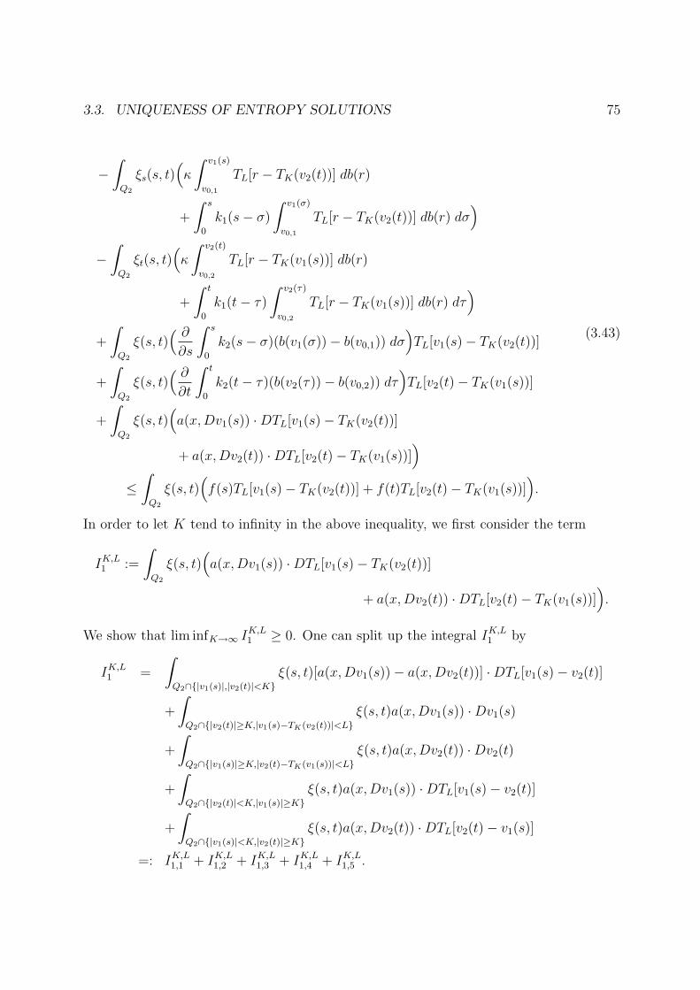
3.3. UNIQUENESS OF ENTROPY SOLUTIONS 75
−∫
Q2
ξs(s, t)(κ
∫ v1(s)
v0,1
TL[r − TK(v2(t))] db(r)
+
∫ s
0
k1(s− σ)
∫ v1(σ)
v0,1
TL[r − TK(v2(t))] db(r) dσ)
−∫
Q2
ξt(s, t)(κ
∫ v2(t)
v0,2
TL[r − TK(v1(s))] db(r)
+
∫ t
0
k1(t− τ)
∫ v2(τ)
v0,2
TL[r − TK(v1(s))] db(r) dτ)
+
∫Q2
ξ(s, t)( ∂∂s
∫ s
0
k2(s− σ)(b(v1(σ))− b(v0,1)) dσ)TL[v1(s)− TK(v2(t))]
+
∫Q2
ξ(s, t)( ∂∂t
∫ t
0
k2(t− τ)(b(v2(τ))− b(v0,2)) dτ)TL[v2(t)− TK(v1(s))]
+
∫Q2
ξ(s, t)(a(x,Dv1(s)) ·DTL[v1(s)− TK(v2(t))]
+ a(x,Dv2(t)) ·DTL[v2(t)− TK(v1(s))])
≤∫
Q2
ξ(s, t)(f(s)TL[v1(s)− TK(v2(t))] + f(t)TL[v2(t)− TK(v1(s))]
).
(3.43)
In order to let K tend to infinity in the above inequality, we first consider the term
IK,L1 :=
∫Q2
ξ(s, t)(a(x,Dv1(s)) ·DTL[v1(s)− TK(v2(t))]
+ a(x,Dv2(t)) ·DTL[v2(t)− TK(v1(s))]).
We show that lim infK→∞ IK,L1 ≥ 0. One can split up the integral IK,L
1 by
IK,L1 =
∫Q2∩|v1(s)|,|v2(t)|<K
ξ(s, t)[a(x,Dv1(s))− a(x,Dv2(t))] ·DTL[v1(s)− v2(t)]
+
∫Q2∩|v2(t)|≥K,|v1(s)−TK(v2(t))|<L
ξ(s, t)a(x,Dv1(s)) ·Dv1(s)
+
∫Q2∩|v1(s)|≥K,|v2(t)−TK(v1(s))|<L
ξ(s, t)a(x,Dv2(t)) ·Dv2(t)
+
∫Q2∩|v2(t)|<K,|v1(s)|≥K
ξ(s, t)a(x,Dv1(s)) ·DTL[v1(s)− v2(t)]
+
∫Q2∩|v1(s)|<K,|v2(t)|≥K
ξ(s, t)a(x,Dv2(t)) ·DTL[v2(t)− v1(s)]
=: IK,L1,1 + IK,L
1,2 + IK,L1,3 + IK,L
1,4 + IK,L1,5 .
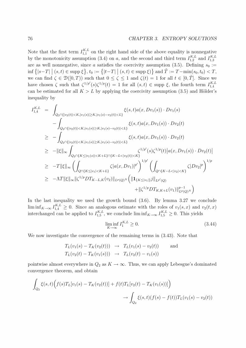
76 CHAPTER 3. ENTROPY SOLUTIONS
Note that the first term IK,L1,1 on the right hand side of the above equality is nonnegative
by the monotonicity assumption (3.4) on a, and the second and third term IK,L1,2 and IK,L
1,3
are as well nonnegative, since a satisfies the coercivity assumption (3.5). Defining s0 :=
inf|s−T |
∣∣ (s, t) ∈ supp ξ, t0 :=
|t−T |
∣∣ (s, t) ∈ supp ξ)
and T := T−min(s0, t0) < T ,
we can find ζ ∈ D([0, T )) such that 0 ≤ ζ ≤ 1 and ζ(t) = 1 for all t ∈ [0, T ]. Since we
have chosen ζ such that ζ1/p′(s)ζ1/p(t) = 1 for all (s, t) ∈ supp ξ, the fourth term IK,L1,4
can be estimated for all K > L by applying the coercivity assumption (3.5) and Holder’s
inequality by
IK,L1,4 =
∫Q2∩|v2(t)|<K,|v1(s)|≥K,|v1(s)−v2(t)|<L
ξ(s, t)a(x,Dv1(s)) ·Dv1(s)
−∫
Q2∩|v2(t)|<K,|v1(s)|≥K,|v1(s)−v2(t)|<Lξ(s, t)a(x,Dv1(s)) ·Dv2(t)
≥ −∫
Q2∩|v2(t)|<K,|v1(s)|≥K,|v1(s)−v2(t)|<Lξ(s, t)a(x,Dv1(s)) ·Dv2(t)
≥ −‖ξ‖∞∫
Q2∩K≤|v1(s)|<K+L∩K−L<|v2(t)|<Kζ1/p′(s)ζ1/p(t)
∣∣a(x,Dv1(s)) ·Dv2(t)∣∣
≥ −T‖ξ‖∞(∫
Q∩K≤|v1|<K+Lζ|a(x,Dv1)|p
′)1/p′ (∫
Q∩K−L<|v2|<Kζ|Dv2|p
)1/p
≥ −ΛT‖ξ‖∞‖ζ1/pDTK−L,K(v2)‖Lp(Q)N
(‖1K≤|v1|j‖Lp′ (Q)
+‖ζ1/pDTK,K+L(v1)‖p−1Lp(Q)N
)In the last inequality we used the growth bound (3.6). By lemma 3.27 we conclude
lim infK→∞ IK,L1,4 ≥ 0. Since an analogous estimate with the roles of v1(s, x) and v2(t, x)
interchanged can be applied to IK,L1,5 , we conclude lim infK→∞ IK,L
1,5 ≥ 0. This yields
lim infK→∞
IK,L1 ≥ 0. (3.44)
We now investigate the convergence of the remaining terms in (3.43). Note that
TL(v1(s)− TK(v2(t))) → TL(v1(s)− v2(t)) and
TL(v2(t)− TK(v1(s))) → TL(v2(t)− v1(s))
pointwise almost everywhere in Q2 as K →∞. Thus, we can apply Lebesgue’s dominated
convergence theorem, and obtain∫Q2
ξ(s, t)(f(s)TL[v1(s)− TK(v2(t))] + f(t)TL[v2(t)− TK(v1(s))]
)→∫
Q2
ξ(s, t)(f(s)− f(t))TL(v1(s)− v2(t))
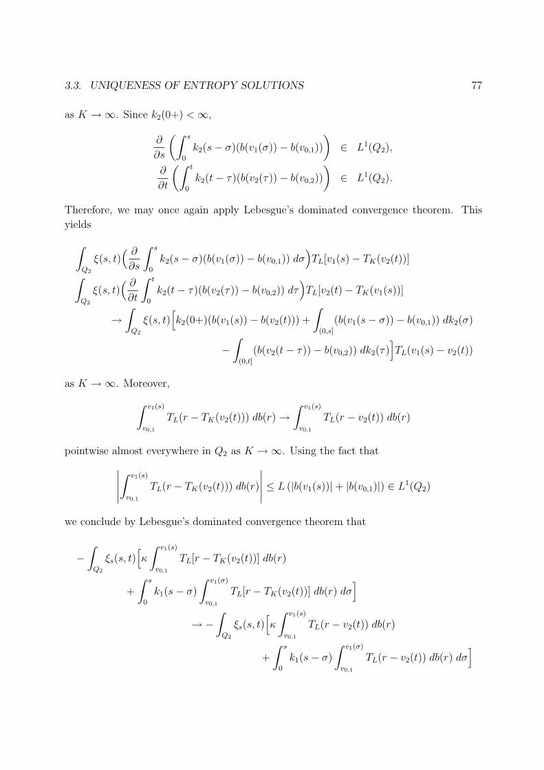
3.3. UNIQUENESS OF ENTROPY SOLUTIONS 77
as K →∞. Since k2(0+) <∞,
∂
∂s
(∫ s
0
k2(s− σ)(b(v1(σ))− b(v0,1))
)∈ L1(Q2),
∂
∂t
(∫ t
0
k2(t− τ)(b(v2(τ))− b(v0,2))
)∈ L1(Q2).
Therefore, we may once again apply Lebesgue’s dominated convergence theorem. This
yields∫Q2
ξ(s, t)( ∂∂s
∫ s
0
k2(s− σ)(b(v1(σ))− b(v0,1)) dσ)TL[v1(s)− TK(v2(t))]∫
Q2
ξ(s, t)( ∂∂t
∫ t
0
k2(t− τ)(b(v2(τ))− b(v0,2)) dτ)TL[v2(t)− TK(v1(s))]
→∫
Q2
ξ(s, t)[k2(0+)(b(v1(s))− b(v2(t))) +
∫(0,s]
(b(v1(s− σ))− b(v0,1)) dk2(σ)
−∫
(0,t]
(b(v2(t− τ))− b(v0,2)) dk2(τ)]TL(v1(s)− v2(t))
as K →∞. Moreover,∫ v1(s)
v0,1
TL(r − TK(v2(t))) db(r) →∫ v1(s)
v0,1
TL(r − v2(t)) db(r)
pointwise almost everywhere in Q2 as K →∞. Using the fact that∣∣∣∣∣∫ v1(s)
v0,1
TL(r − TK(v2(t))) db(r)
∣∣∣∣∣ ≤ L (|b(v1(s))|+ |b(v0,1)|) ∈ L1(Q2)
we conclude by Lebesgue’s dominated convergence theorem that
−∫
Q2
ξs(s, t)[κ
∫ v1(s)
v0,1
TL[r − TK(v2(t))] db(r)
+
∫ s
0
k1(s− σ)
∫ v1(σ)
v0,1
TL[r − TK(v2(t))] db(r) dσ]
→ −∫
Q2
ξs(s, t)[κ
∫ v1(s)
v0,1
TL(r − v2(t)) db(r)
+
∫ s
0
k1(s− σ)
∫ v1(σ)
v0,1
TL(r − v2(t)) db(r) dσ]
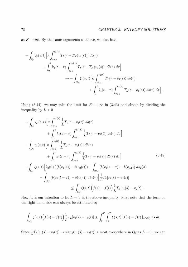
78 CHAPTER 3. ENTROPY SOLUTIONS
as K →∞. By the same arguments as above, we also have
−∫
Q2
ξt(s, t)[κ
∫ v2(t)
v0,2
TL[r − TK(v1(s))] db(r)
+
∫ t
0
k1(t− τ)
∫ v2(τ)
v0,2
TL[r − TK(v1(s))] db(r) dτ]
→ −∫
Q2
ξt(s, t)[κ
∫ v2(t)
v0,2
TL(r − v1(s)) db(r)
+
∫ t
0
k1(t− τ)
∫ v2(τ)
v0,2
TL(r − v1(s)) db(r) dτ].
Using (3.44), we may take the limit for K → ∞ in (3.43) and obtain by dividing the
inequality by L > 0
−∫
Q2
ξs(s, t)[κ
∫ v1(s)
v0,1
1
LTL[r − v2(t)] db(r)
+
∫ s
0
k1(s− σ)
∫ v1(σ)
v0,1
1
LTL[r − v2(t)] db(r) dσ
]−∫
Q2
ξt(s, t)[κ
∫ v2(t)
v0,2
1
LTL[r − v1(s)] db(r)
+
∫ t
0
k1(t− τ)
∫ v2(τ)
v0,2
1
LTL[r − v1(s)] db(r) dτ
]+
∫Q2
ξ(s, t)[k2(0+)(b(v1(s))− b(v2(t))) +
∫(0,s]
(b(v1(s− σ))− b(v0,1)) dk2(σ)
−∫
(0,t]
(b(v2(t− τ))− b(v0,2)) dk2(τ)] 1
LTL[v1(s)− v2(t)]
≤∫
Q2
ξ(s, t)(f(s)− f(t)
) 1
LTL[v1(s)− v2(t)].
(3.45)
Now, it is our intention to let L→ 0 in the above inequality. First note that the term on
the right hand side can always be estimated by
∫Q2
ξ(s, t)(f(s)− f(t)
) 1
LTL[v1(s)− v2(t)] ≤
∫ T
0
∫ T
0
ξ(s, t)‖f(s)− f(t)‖L1(Ω) ds dt.
Since 1LTL[v1(s)− v2(t)] → sign0(v1(s)− v2(t)) almost everywhere in Q2 as L→ 0, we can
3.3. UNIQUENESS OF ENTROPY SOLUTIONS 79
apply Lebesgue’s dominated convergence theorem and conclude∫Q2
ξ(s, t)(k2(0+)(b(v1(s))− b(v2(t))) +
∫(0,s]
(b(v1(s− σ))− b(v0,1)) dk2(σ)
−∫
(0,t]
(b(v2(t− τ))− b(v0,2)) dk2(τ)) 1
LTL[v1(s)− v2(t)]
→∫
Q2
ξ(s, t)(k2(0+)(b(v1(s))− b(v2(t))) +
∫(0,s]
(b(v1(s− σ))− b(v0,1)) dk2(σ)
−∫
(0,t]
(b(v2(t− τ))− b(v0,2)) dk2(τ))sign0(v1(s)− v2(t)) =: I2
as L→ 0. Note that (b(v1(s))− b(v2(t)))sign0(v1(s)− v2(t)) = |b(v1(s)− b(v2(t))| almost
everywhere in Q2, since b is nondecreasing and b(0) = 0. Thus, using the fact that dk2 is
a nonpositive measure on (0,∞), we obtain
I2 =
∫Q2
ξ(s, t)(k2(0+)(b(v1(s))−b(v2(t)))+
∫(0,min(s,t)]
(b(v1(s−τ))−b(v2(t−τ))) dk2(τ)
+ 1t<s
∫(t,s]
(b(v1(s− σ))− b(v0,1)) dk2(σ)
− 1s<t
∫(s,t]
(b(v2(t− τ))− b(v0,2)) dk2(τ))sign0(v1(s)− v2(t))
≥∫ T
0
∫ T
0
ξ(s, t)(k2(0+)‖b(v1(s))− b(v2(t))‖L1(Ω)
+
∫(0,min(s,t)]
‖b(v1(s− τ))− b(v2(t− τ))‖L1(Ω) dk2(τ)
+ 1t<s
∫(t,s]
‖b(v1(s− σ))− b(v0,1)‖L1(Ω) dk2(σ)
+ 1s<t
∫(s,t]
‖b(v2(t− τ))− b(v0,2)‖L1(Ω) dk2(τ)).
Thus, it remains to investigate the convergence of the first two integrals in (3.45) as L→ 0.
Therefore, we note that∫ v1(s)
v0,1
1
LTL[r − v2(t)] db(r) →
∫ v1(s)
v0,1
sign0[r − v2(t)] db(r)
=∣∣b(v1(s))− b(v2(t))
∣∣− ∣∣b(v2(t))− b(v0,1)∣∣
almost everywhere in Q2 as L→ 0. Since, moreover,∫ v1(s)
v0,1
1
LTL[r − v2(t)] db(r) ≤
∣∣b(v1(s))− b(v2(t))∣∣+ ∣∣b(v2(t))− b(v0,1)
∣∣ ∈ L1(Q2),
80 CHAPTER 3. ENTROPY SOLUTIONS
Lebesgue’s dominated convergence theorem yields
−∫
Q2
ξs(s, t)(κ
∫ v1(s)
v0,1
1
LTL[r − v2(t)] db(r)
+
∫ s
0
k1(s− σ)
∫ v1(σ)
v0,1
1
LTL[r − v2(t)] db(r) dσ
)→ −
∫ T
0
∫ T
0
ξs(s, t)(κ(‖b(v1(s))− b(v2(t))‖L1(Ω) − ‖b(v2(t))− b(v0,1)‖L1(Ω)
)+
∫ s
0
k1(s− σ)(‖b(v1(σ))− b(v2(t))‖L1(Ω) − ‖b(v2(t))− b(v0,1)‖L1(Ω)
)dσ)ds dt.
Note that
κ
∫ T
0
∫ T
0
ξs(s, t)‖b(v2(t))− b(v0,1)‖ ds dt = −κ∫ T
0
ξ(0, t)‖b(v2(t))− b(v0,1)‖ dt.
Using essentially the same arguments as above in order to estimate the limit for L→ 0 of
−∫
Q2
ξt(s, t)(κ
∫ v2(t)
v0,2
1
LTL[r − v1(s)] db(r)
+
∫ t
0
k1(t − τ)
∫ v2(τ)
v0,2
1
LTL[r − v1(s)] db(r) dτ
)we conclude for u1 := b(v1), u2 := b(v2) and u0 := b(v0,1) = b(v0,2) by taking the limit for
L→ 0 in (3.45)
−∫ T
0
∫ T
0
ξs(s, t)(κ‖u1(s)− u2(t)‖+
∫ s
0
k1(s− σ)‖u1(σ)− u2(t)‖ dσ)ds dt
−∫ T
0
∫ T
0
ξt(s, t)(κ‖u1(s)− u2(t)‖+
∫ t
0
k1(t− τ)‖u1(s)− u2(τ)‖ dτ)ds dt
≤∫ T
0
∫ T
0
ξ(s, t)(F (s, t)+k1(s)‖u2(t)−u0‖L1(Ω)+k1(t)‖u1(s)−u0‖L1(Ω)
)ds dt
+κ
(∫ T
0
ξ(0, t)‖u2(t)− u0‖L1(Ω) dt+
∫ T
0
ξ(s, 0)‖u1(s, 0)− u0‖L1(Ω) ds
),
(3.46)
where
F (s, t) := ‖f(s)− f(t)‖L1(Ω)
− k2(0+)‖u1(s)− u2(t)‖L1(Ω) −∫
(0,min(s,t)]
‖u1(s− τ)− u2(t− τ)‖L1(Ω) dk2(τ)
−1t<s
∫(t,s]
‖u1(s−σ)−u0‖L1(Ω) dk2(σ)−1s<t
∫(s,t]
‖u2(t−τ)−u0‖L1(Ω) dk2(τ).
3.3. UNIQUENESS OF ENTROPY SOLUTIONS 81
We remark that the above inequality (3.46) is equivalent to [CGL96, Equation (45)]. Thus,
to complete the proof, we might follow exactly the arguments as developed in [CGL96].
But in order to omit the continuity assumption at t = 0 for one of the entropy solutions, we
will give a somewhat different proof without applying the methods of [CGL96, Lemma 10].
This means that we will not use the existence of a nonnegative measure µ on [0,∞)×[0,∞)
such that
∂
∂s
(κµ(s, t) +
∫ s
0
k(s− σ)dµ(σ, t)
)+∂
∂t
(κµ(s, t) +
∫ t
0
k(t− τ)dµ(s, τ)
)= δ0(s, t)
holds in the sense of distributions, i.e. for all ξ ∈ D([0, T )× [0, T ))
−∫ T
0
∫ T
0
(κξs(s, t) +
∫ T−s
0
k(σ)ξs(σ + s, t) dσ
)dµ(s, t)
−∫ T
0
∫ T
0
(κξt(s, t) +
∫ T−t
0
k(τ)ξt(s, t+ τ) dτ
)dµ(s, t) = ξ(0, 0).
We define y(s, t) := ‖u1(s) − u1(t)‖L1(Ω) for s, t > 0. Moreover, let y(s, 0) := ‖u1(s) −u0‖L1(Ω), and y(0, t) := ‖u0 − u2(t)‖L1(Ω) for all s, t ≥ 0, and y(s, t) = 0 for all s, t ∈ Rsuch that s < 0 or t < 0. Since (3.46) holds for all combinations k1, k2 ∈ L1(0, T ) of
nonnegative nonincreasing functions such that k = k1 + k2 and k2(0+) <∞, we choose a
sequence k1,nn∈N such that
k1,n(t) := max
(0, k(t)− k
(1
n
)). (3.47)
Then, obviously k1,n → 0 in L1(0, T ) and k2,n := k − k1,n → k in L1(0, T ). We choose a
sequence %εε>0 of mollifiers on R such that supp %ε ⊂ [0, ε] and %ε → δ0 in D′(R) as
ε→ 0. Defining ξε(s, t) := %ε(s− t)φ(t) for φ ∈ D([0, T )) with φ ≥ 0, it is easy to see that
ξε ∈ D([0, T )× [0, T )) with ξε ≥ 0 for ε > 0 small enough.
By (3.46) we now conclude for all n ∈ N and all ε > 0 small enough
Jε,n1 + Jε,n
2 ≤ Jε,n3 + Jε,n
4 + Jε5 + Jε
6 (3.48)
where
Jε,n1 := −
∫ T
0
∫ T
0
(ξε)s(s, t)
(κy(s, t) +
∫ s
0
k1,n(s− σ)y(σ, t) dσ
)ds dt
−∫ T
0
∫ T
0
(ξε)t(s, t)
(κy(s, t) +
∫ t
0
k1,n(t− τ)y(s, τ) dτ
)ds dt,
Jε,n2 :=
∫ T
0
∫ T
0
ξε(s, t)
(k2,n(0+)y(s, t) +
∫(0,min(s,t)]
y(s− τ, t− τ) dk2,n(τ)
)ds dt,
82 CHAPTER 3. ENTROPY SOLUTIONS
Jε,n3 := −
∫ T
0
∫ T
0
ξε(s, t)1t<s
∫(t,s]
y(s− σ, 0) dk2,n(σ) ds dt
−∫ T
0
∫ T
0
ξε(s, t)1s<t
∫(s,t]
y(0, t− τ) dk2,n(τ) ds dt,
Jε,n4 :=
∫ T
0
∫ T
0
ξε(s, t)(k1,n(s)y(0, t) + k1,n(t)y(s, 0)
)ds dt,
Jε5 :=
∫ T
0
∫ T
0
ξε(s, t)‖f(s)− f(t)‖L1(Ω) ds dt,
and
Jε6 := κ
(∫ T
0
ξε(0, t)y(0, t) dt+
∫ T
0
ξε(s, 0)y(s, 0) ds
).
It is our intention to first let n → ∞ and then ε → 0+ in (3.48). Since (ξε)s(s, t) =
%ε′(s− t)φ(t) and (ξε)t(s, t) = −%ε
′(s− t)φ(t) + %ε(s− t)φ′(t), we conclude
limε→0+
limn→∞
Jε,n1 = − lim
ε→0+κ
∫ T
0
∫ T
0
%ε(s− t)φ′(t)y(s, t) ds dt = −κ∫ T
0
φ′(t)y(t, t) dt.
Here, we used the fact that k1,n → 0 in L1(0, T ) as n→∞. For Jε,n2 we use the transfor-
mation (η, ν) 7→ (η + ν2, η − ν
2) = (s, t) of the integral. Thus
Jε,n2 =
∫ 2T
−2T
∫ T−|ν/2|
|ν/2|ξε(η + ν
2, η − ν
2)(k2,n(0+)y(η + ν
2, η − ν
2)
+
∫(0,η]
y(η + ν2− τ, η − ν
2− τ) dk2,n(τ)
)dη dν
= −∫ 2T
−2T
∫ T−|ν/2|
|ν/2|%ε(ν)φ
′(η − ν2)
∫ η
0
k2,n(η − τ)y(τ + ν2, τ − ν
2) dτ dη dν.
We used the fact that, by definition, y(s, t) = 0 for s < 0 or t < 0. Note, moreover, that
the boundary terms are zero. Since k2,n → k in L1(0, T ) as n→∞, we can conclude
limε→0+
limn→∞
Jε,n2 = −
∫ T
0
φ′(t)
∫ t
0
k(t− τ)y(τ, τ) dτ dt.
In order to estimate Jε,n3 we use the assumption limt→0+ ‖u1(t)−u0‖L1(Ω) = 0 and the fact
that ξε(s, t) = %ε(s− t)φ(t) = 0 for s < t and obtain
0 ≤ Jε,n3 ≤
(sup
σ∈[0,ε]
y(σ, 0)
)∫ T
0
∫ T
t
ξε(s, t) (k2,n(t)− k2,n(s)) ds dt→ 0
3.4. EXISTENCE OF ENTROPY SOLUTIONS 83
as n→∞ and ε→ 0+. Note that
limn→∞
Jε,n4 = lim
n→∞
∫ T
0
∫ T
0
ξε(s, t)(k1,n(s)y(0, t) + k1,n(t)y(s, 0)
)ds dt = 0,
since k1,n → 0 in L1(0, T ) as n→∞, and that
limε→0
∫ T
0
ξε(s, t)‖f(s)− f(t)‖L1(Ω) = 0
almost everywhere for t ∈ [0, T ). Hence, limε→0+ Jε5 = 0. Finally, since limt→0 ‖u1(t) −
u0‖L1(Ω) = 0 and ξε(0, t) = %ε(0− t)φ(t) = 0 for t ≥ 0, we obtain
limε→0+
Jε6 = lim
ε→0+κ
∫ ε
0
%ε(s)φ(0)y(s, 0) ds = 0.
Combining the above results, we conclude by (3.48)
−∫ T
0
φ′(t)
(κy(t, t) +
∫ t
0
k(t− τ)y(τ, τ) dτ
)dt ≤ 0
for all φ ∈ D([0, T )) with φ ≥ 0. The convolution of this inequality with the completely
positive measure α associated to (κ, k) and defined by (A.2) yields
y(t, t) ≤ 0 (3.49)
in the sense of distributions and thus almost everywhere in (0, T ). Therefore, we have
shown that
b(v1) = u1 = u2 = b(v2)
almost everywhere in Q = (0, T )× Ω.
3.4 Existence of entropy solutions
In this section we prove the existence of entropy solutions for the non-degenerated history
dependent problem
∂
∂t
(κ(u(t, x)− u0(x)
)+
∫ t
0
k(t− s)(u(s, x)− u0(x)
)ds)
= div a(x,Du(t, x)) + f(t, x) for (t, x) ∈ Q := (0, T )× Ω,
u(0, ·) = b(v0) in Ω,
u(t, x) = 0 for (t, x) ∈ Γ := (0, T )× ∂Ω.
(3.50)
84 CHAPTER 3. ENTROPY SOLUTIONS
Here, we assume that (3.4)-(3.6) and (3.8),(3.9) hold. In particular, we show that the
generalized solution of an associated abstract Volterra equation in L1(Ω) is an entropy
solution of (3.50).
To this end, define the operator A∞ ⊂ L1(Ω)× L1(Ω) by
(v, w) ∈ A∞ :⇔ v ∈ W 1,p0 (Ω) ∩ L∞(Ω), w ∈ L1(Ω) and∫
Ω
a(x,Dv) · φ =
∫Ω
wφ
for all φ ∈ W 1,p0 (Ω) ∩ L∞(Ω).
Then A∞ is a completely-accretive operator in L1(Ω) with R(I + λA∞) ⊃ L∞(Ω) for all
λ > 0, and its closure A := A∞ is an m-completely-accretive operator in L1(Ω) which can
be characterized by
(v, w) ∈ A ⇔ v, w ∈ L1(Ω) and TK(v) ∈ W 1,p0 (Ω) for all K > 0 and∫
Ω
a(x,Dv) ·DTK(v − φ) ≤∫
Ω
wTK(v − φ)
for all φ ∈ W 1,p0 (Ω) ∩ L∞(Ω), K > 0.
(3.51)
Note that according to the coercivity assumption (3.5) one has 0 ∈ A(0). To see this use
tφ with t ∈ R and φ ∈ W 1,p0 (Ω) ∩ L∞(Ω) as a test function. Thus,
t
∫Ω
a(x, tDφ) ·Dφ ≥ 0.
Dividing the above inequality by t and letting t → 0+ and t → 0− we conclude by the
hemicontinuity of A : W 1,p0 (Ω) → W−1,p′ with A(u) := − div a(x,Du) that∫
Ω
a(x, 0) ·Dφ = 0
for all φ ∈ W 1,p0 (Ω) ∩ L∞(Ω), i.e., that a(x, 0) = 0 a.e. for x ∈ Ω.
By [CGL96], [Gri85] respectively, we already know that for all u0 ∈ D(A) = L1(Ω) and all
f ∈ L1(0, T ;L1(Ω)) = L1(Q) the abstract Volterra equation
d
dt
(κ(u(t)− u0) +
∫ t
0
k(t− s)(u(s)− u0) ds)
+ Au(t) 3 f(t) (3.52)
admits a unique generalized solution u ∈ L1(Q). But it is not clear in which sense this
generalized solution satisfies the equation (3.50). Therefore, we are interested in an approx-
imating sequence of solutions, which satisfy the abstract Volterra equation almost every-
where for t ∈ [0, T ) and, moreover, are weak solutions of (3.50). We define approximating
sequences u0,nn∈N ⊂ D(A)∩L∞(Ω) and fnn∈N ⊂ W 1,p0 (0, T ;L1(Ω))∩L∞(0, T ;L∞(Ω))
3.4. EXISTENCE OF ENTROPY SOLUTIONS 85
with u0,n → u0 in L1(Ω) and fn → f in L1(Q) as n→∞. Then, by proposition 2.11 and
proposition 2.14, the generalized solution un ∈ L1(0, T, L1(Ω)) of the abstract Volterra
equation (3.52) with initial value u0,n and right hand side fn is a strong solution for all
n ∈ N, i.e. the mapping
(0, T ) 3 t 7→ κ(un(t)− u0,n) +
∫ t
0
k(t− s)(un(s)− u0,n) ds ∈ L1(Ω)
is absolutely continuous and differentiable almost everywhere with(un(t), fn(t)− d
dt
(κ(un(t)− u0,n) +
∫ t
0
k(t− s)(un(s)− u0,n) ds
))∈ A
almost everywhere for t ∈ [0, T ). By the continuous dependence of the solution on the
data, [Gri85, Theorem 5], we already know that un → u in L1(Q) as n→∞.
We first show that for the above choices of u0,n and fn the generalized solution un is also
a weak solution of
d
dt
(κ(un(t, x)− u0,n(x)) +
∫ t
0
k(t− s)(un(s, x)− u0,n(x)) ds)
−diva(x,Dun(t, x)) = fn(t, x) (t, x) ∈ Q
u(0, ·) = u0,n in Ω,
u(t, x) = 0 for (t, x) ∈ Γ.
(3.53)
To this end, we will need the following proposition which can be found in [CGL96, Propo-
sition 5].
Proposition 3.28. Let A be an m-accretive operator in a Banach space X, u0 ∈ D(A)
and f ∈ L1(0, T ;X). We assume that κ, k satisfies (3.8) and that u is the generalized
solution of (3.52). Moreover, let Y be a Banach space such that
(i) the set x ∈ X ∩ Y∣∣ ‖x‖Y ≤ 1 is closed in X,
(ii) for every x ∈ X ∩ Y and every λ > 0 we have ‖(I + λA)−1x‖Y ≤ ‖x‖Y ,
(iii) u0 ∈ X ∩ Y and ‖f(·)‖Y ∈ L1(0, T ).
Then
‖u(t)‖Y ≤ ‖u0‖Y +
∫[0,t]
‖f(t− s)‖Y dα(s)
almost everywhere for t ∈ [0, T ), where α is the completely positive measure associated to
κ, k.
86 CHAPTER 3. ENTROPY SOLUTIONS
Note that, since Ω is a bounded domain, L∞(Ω) ⊂ L1(Ω). Moreover, the unit ball BL∞(Ω)
of L∞(Ω) is closed in L1(Ω). Since the operator A defined by (3.51) satisfies 0 ∈ A(0),
we have ‖(I + λA)−1f‖∞ ≤ ‖f‖∞ for all f ∈ L∞(Ω). Here, we used the fact that the
resolvent JAλ of A is nonexpansive in L∞(Ω), since A is completely accretive. Applying
the above proposition, we can show that generalized solutions satisfy the equation (3.50)
in the weak sense if the data are sufficiently regular.
Proposition 3.29. Let (3.4)-(3.6) and (3.8), (3.9) be satisfied and let the m-completely
accretive operator A be defined by (3.51). Assume that u0 ∈ D(A) ∩ L∞(Ω) and f ∈W 1,1(0, T ;L1(Ω)) ∩ L∞(0, T ;L∞(Ω)). Then the generalized solution u of the abstract
Volterra equation (3.52) satisfies for a.e. t ∈ [0, T )
u(t) ∈ W 1,p0 (Ω) ∩ L∞(Ω),
∂
∂t
(κ(u− u0) + k ∗ (u− u0)
)∈ L1(0, T ;L1(Ω)) = L1(Q),
and, moreover,∫Ω
∂
∂t
(κ(u(t)− u0) +
∫ t
0
k(t− s)(u(s)− u0) ds
)φ
+
∫Ω
a(x,Du(t)) ·Dφ =
∫Ω
f(t)φ
(3.54)
for all φ ∈ W 1,p0 (Ω) ∩ L∞(Ω) almost everywhere for t ∈ [0, T ).
Proof. Let u be the generalized solution of (3.52) for the data u0 ∈ D(A)∩L∞(Ω) and f ∈W 1,1(0, T ;L1(Ω))∩L∞(Q). We first remark that, by W 1,1(0, T ;L1(Ω)) ⊂ BV (0, T ;L1(Ω))
and proposition 2.11, u is a strong solution of (3.52) in case κ = 0. Moreover, if κ > 0,
then by proposition 2.14 we also conclude that u is a strong solution. In particular
d
dt
(κ(u− u0) + k ∗ (u− u0)
)∈ L1(0, T ;L1(Ω)),
and u(t) ∈ D(A) almost everywhere for t ∈ [0, T ). By the characterization of the operator
A in (3.51), we obtain TK(u(t)) ∈ W 1,p0 (Ω) for all K > 0 almost everywhere for t ∈ [0, T ),
and∫Ω
∂
∂t
(κ(u(t)− u0) +
∫ t
0
k(t− s)(u(s)− u0) ds
)TK(u− φ)
+
∫Ω
a(x,Du(t)) ·DTK(u− φ) ≤∫
Ω
f(t)TK(u− φ)
(3.55)
for all K > 0 and all φ ∈ W 1,p0 (Ω) ∩ L∞(Ω) almost everywhere for t ∈ [0, T ). We now
use the assumptions u0 ∈ L∞(Ω) and f ∈ L∞(0, T ;L∞(Ω)) to conclude by proposition
3.28 that u ∈ L∞(0, T ;L∞(Ω)) ⊂ L∞(Q). Thus, taking K := ‖u‖∞, we easily see that
u(t) = TK(u(t)) ∈ W 1,p0 (Ω) ∩ L∞(Ω) almost everywhere for t ∈ [0, T ).
3.4. EXISTENCE OF ENTROPY SOLUTIONS 87
Let ξ ∈ W 1,p0 (Ω) ∩ L∞(Ω). Then using φ := u(t) − ξ and K := ‖u‖∞ + ‖ξ‖∞ in (3.54),
gives∫Ω
∂
∂t
(κ(u(t)− u0) +
∫ t
0
k(t− s)(u(s)− u0) ds
)ξ +
∫Ω
a(x,Du(t)) ·Dξ ≤∫
Ω
f(t)ξ
almost everywhere for t ∈ [0, T ). Combining this result with the inequality one obtains
when using φ := u(t) + ξ and K := ‖u‖∞ + ‖ξ‖∞ in (3.54) yields the assertion.
By the above proposition we conclude that the generalized solution un of the abstract
Volterra equation (3.52) with data u0,n ∈ D(A) ∩ L∞(Ω) and fn ∈ W 1,1(0, T ;L1(Ω)) ∩L∞(0, T ;L∞(Ω)) is a weak solution of (3.53).
We use this sequence of weak solutions in order to show that the generalized solution of
(3.52) for u0 ∈ L1(Ω) and f ∈ L1(Q) is an entropy solution of (3.50). By the continuous
dependence on the data, see [Gri85, Theorem 5], we already know that un → u in L1(Q),
since we assumed u0,n → u0 in L1(Ω) and fn → f in L1(Q) as n → ∞. Thus, the main
task is to obtain convergence of the sequence DTK(un)n∈N of gradients of TK(un) for all
K > 0. Therefore, we first show the boundedness of the sequence DTK(un)n in Lp(Q)N
by an a-priori estimate. This implies the weak convergenceDTK(un) DTK(u) in Lp(Q)N
of a subsequence. Minty’s trick then implies div a(x,DTK(un)) div a(x,DTK(u)) in
Lp′(0, T ;W−1,p′(Ω)).
Theorem 3.30. Let (3.4)-(3.6) and (3.8), (3.9) be satisfied. Let the operator A be defined
by (3.51) and let u0 ∈ L1(Ω) and f ∈ L1(Q). Then the generalized solution u of (3.52) is
an entropy solution of (3.50).
Proof. We choose sequences u0,nn∈N ⊂ D(A)∩L∞(Ω) and fnn∈N ⊂ W 1,1(0, T ;L1(Ω))∩L∞(0, T ;L∞(Ω)) with u0,n → u0 in L1(Ω) and fn → f in L1(Q) as n → ∞. Then, as
shown in proposition 3.29, the generalized solution un ∈ L1(Q) of (3.52) with data u0,n
and fn satisfies∫Ω
∂
∂t
(κ(un(t)− u0,n) +
∫ t
0
k(t− s) (un(s)− u0,n) ds
)φ
+
∫Ω
a(x,Dun(t)) ·Dφ =
∫Ω
f(t)φ
(3.56)
for all φ ∈ W 1,p0 (Ω) ∩ L∞(Ω). Moreover, u(t) ∈ W 1,p
0 (Ω) almost everywhere for t ∈ [0, T ).
In the following let K > 0 be fixed. In order to obtain an a-priori estimate on the gradients
of the approximating solutions un we take the truncation TK(un) of un for K > 0 as a test
function in (3.56) and integrate this equation over (0, T ).
88 CHAPTER 3. ENTROPY SOLUTIONS
λ
∫Q
|DTK(un)|p ≤∫
Q
a(x,Dun) ·DTK(un)
=
∫Q
fnTK(un)−∫
Q
∂
∂t
[κ(un(t)− u0,n)
+
∫ t
0
k(t− s) (un(s)− u0,n) ds]TK(un(t))
≤∫
Q
fnTK(un)− κ
∫Ω
∫ un(T )
u0,n
TK(r) dr dx
−∫ T
0
k(T − s)
∫Ω
∫ un(s)
u0,n
TK(r) dr dx ds
≤ K‖fn‖L1(Q) +K(κ+ ‖k‖L1(0,T )
)‖u0,n‖L1(Ω).
(3.57)
Here, we used the coercivity assumption (3.5) and the Kato inequality, proposition 3.23.
Moreover, we used the fact that∫ s
0TK(r) dr ≥ 0 for all s ∈ R. Thus, DTK(un)n∈N
is a bounded sequence in Lp(Q)N . By Poincare’s inequality TK(un)n is a bounded
sequence in Lp(0, T ;W 1,p0 (Ω)), and thus admits a weakly convergent subsequence, i.e.,
TK(un) vK weakly in Lp(0, T ;W 1,p0 (Ω)) as n → ∞ with some vK ∈ Lp(0, T ;W 1,p
0 (Ω)).
The continuous dependence of the solution on the data, according to [Gri85, Theorem 5],
implies un → u in L1(Q), since u0,n → u0 in L1(Ω) and fn → f in L1(Q). This implies
that TK(un) → TK(u) in L1(Q). Using test functions it is easy to see that TK(u) = vK .
Thus, we have TK(un) TK(u) weakly in Lp(0, T ;W 1,p0 (Ω)) for a subsequence. Since the
above argument holds for all subsequences of TK(un)n, we conclude TK(un) TK(u)
weakly in Lp(0, T ;W 1,p0 (Ω)) for the sequence itself. Moreover, by the growth bound (3.6)∫
Q
|a(x,DTK(un))|p′ ≤ Λp′(T 1/p′‖j‖Lp′ (Ω) + ‖DTK(un)‖p/p′
Lp(Q)N
)p′
. (3.58)
Thus, the sequence a(x,DTK(un))n∈N is bounded in Lp′(Q)N and admits a weakly con-
vergent subsequence in Lp′(Q)N . Without loss of generality we assume a(x,DTK(un))
σK weakly in Lp′(Q)N with some σK ∈ Lp′(Q)N .
In order to show that div σK = div a(x,DTK(u)), we want to apply a pseudo-monotonicity
argument. Therefore, we need the following convergence result
limL→0
limm→∞
limn→∞
∫Q
[a(x,DTK(um))− a(x,DTK(un)] ·DTL [TK(um)− TK(un)] = 0. (3.59)
To show (3.59), we use the following decomposition of the above integral:∫Q
[a(x,DTK(um))− a(x,DTK(un))] ·DTL (TK(um)− TK(un))
3.4. EXISTENCE OF ENTROPY SOLUTIONS 89
=
∫Q∩|um|<K,|un|<K
[a(x,Dum)− a(x,Dun)] ·DTL(um − un)
+
∫Q∩|um|<K,|un|≥K
a(x,Dum) ·DTL(um − sign0(un)K)
+
∫Q∩|um|≥K,|un|<K
a(x,Dun) ·DTL(un − sign0(um)K)
= IK,Lm,n + JK,L
m,n + JK,Ln,m .
By the monotonicity assumption (3.4) it is obvious that
IK,Lm,n ≤
∫Q
[a(x,Dum)− a(x,Dun)] ·DTL (um − un) .
Therefore we can apply (3.56) with the test function φ = TL(um − un) for um and for un
in order to compare these solutions. Adding both equalities and integrating over (0, T )
yields
IK,Lm,n ≤
∫Q
[a(x,Dum)− a(x,Dun)] ·DTL(um − un)
≤ −∫
Q
∂
∂t
[κ (um(t)− un(t))
+
∫ t
0
k(t− s) (um(s)− un(s)) ds]TL(um(t)− un(t))
+
∫Q
k(t)(u0,m − u0,n)TL(um(t)− un(t)) +
∫Q
(fm − fn)TL(um − un)
≤ −κ∫
Ω
um(T )−un(T )∫0
TL(r) dr dx−∫ T
0
k(T − s)
∫Ω
um(s)−un(s)∫0
TL(r) dr dx ds
+L(κ+ ‖k‖L1(0,T ))‖u0,m − u0,n‖L1(Ω)) + L‖fm − fn‖L1(Q)
≤ L((κ+ ‖k‖L1(0,T ))‖u0,m − u0,n‖L1(Ω) + ‖fm − fn‖L1(Q)
).
Here, we applied the Kato inequality, corollary 3.24. By u0,n → u0 in L1(Ω) and fn → f
in L1(Q) as n→∞, we obtain
limL→0
limm→∞
limn→∞
IK,Lm,n = 0.
We claim that
limL→0
limm→∞
limn→∞
JK,Lm,n = 0. (3.60)
90 CHAPTER 3. ENTROPY SOLUTIONS
The term JK,Lm,n can be rewritten in the form
JK,Lm,n =
∫Q∩|um|<K,K≤un
a(x,Dum) ·DTL(um −K))
+
∫Q∩|um|<K,un≤−K
a(x,Dum) ·DTL(um +K))
=
∫Q∩|um|<K,K≤un,|um−K|<L
a(x,Dum) ·Dum
+
∫Q∩|um|<K,un≤−K,|um+K|<L
a(x,Dum) ·Dum.
By the coercivity assumption (3.5) it is clear that a(x,Dum) ·Dum ≥ 0 almost everywhere
on Q. Thus, we might develop an estimate on JK,Lm,n by increasing the set of integration.
Therefore, note that |um| < K and |um − K| < L implies that K − L < um < K.
Analogously, |um| < K and |um +K| < L implies that −K < um < −K + L. This yields
|um| < K, |un| ≥ K, |um − TK(un)| < L= |um| < K,K ≤ un, |um −K| < L ∪ |um| < K, un ≤ −K, |um +K| < L⊂ K − L < um < K ∪ −K < um < −K + L .
We now define for K2 > K1 ≥ 0 the truncation function TK1,K2 : R → R by TK1,K2(r) :=
TK2(r) − TK1(r). Since the above inclusion holds, and due to the coercivity assumption
(3.5), one obtains the estimate
JK,Lm,n ≤
∫Q
a(x,Dum) ·DTK−L,K(um). (3.61)
Again, using the fact that um satisfies (3.56) we can conclude for 0 < L ≤ K by using the
test function TK−L,K(um) and integrating the equality over (0, T )∫Q
a(x,Dum) ·DTK−L,K(um)
=
∫Q
fmTK−L,K(um)
−∫
Q
∂
∂t
[κ (um(t)− u0,m)
+
∫ t
0
k(t− s) (um(s)− u0,m) dr ds]TK−L,K(um(t))
≤∫
Q
fmTK−L,K(um)− κ
∫Ω
∫ um(T )
u0,m
TK−L,K(r) dr dx
−∫ T
0
k(T − s)
∫Ω
∫ um(s)
u0,m
TK−L,K(r) dr dx ds
≤ L‖fn‖L1(Q) + L(κ+ ‖k‖L1(0,T )
)‖u0,m‖L1(Ω).
3.4. EXISTENCE OF ENTROPY SOLUTIONS 91
Here, we once again applied the Kato inequality, proposition 3.23. Inequality (3.61), and
the fact that u0,mm is a bounded sequence in L1(Ω), and that fmm is a bounded
sequence in L1(Q) imply (3.60).
By an analogous estimate, we obtain
limL→0
limm→∞
limn→∞
JK,Ln,m = 0.
Thus, combining the above results yields (3.59).
In the next step our main goal is to show that div a(x,DTK(u)) = div σK by using
Minty’s trick. Therefore, let φ ∈ Lp(0, T ;W 1,p0 (Ω)) be arbitrary. Then, by (3.59), we
obtain
2
∫Q
σK ·Dφ = limL→0
limm→∞
limn→∞
[ ∫Q
a(x,DTK(um)) · (DTL(TK(um)− TK(un)) +Dφ)
+
∫Q
a(x,DTK(un)) · (DTL(TK(un)− TK(um)) +Dφ)].
Thus,
2
∫Q
σK ·Dφ = limL→0
limm→∞
limn→∞
[∫
Q∩|TK(um)−TK(un)|<La(x,DTK(um)) ·D [TK(um)− TK(un) + φ]
+
∫Q∩|TK(um)−TK(un)|≥L
a(x,DTK(um)) ·Dφ
+
∫Q∩|TK(um)−TK(un)|<L
a(x,DTK(un)) ·D [TK(un)− TK(um) + φ]
+
∫Q∩|TK(um)−TK(un)|≥L
a(x,DTK(un)) ·Dφ]
= limL→0
limm→∞
limn→∞
(IK,Lm,n + JK,L
m,n + IK,Ln,m + JK,L
n,m
).
(3.62)
For the second term JK,Lm,n we can apply the following estimate∣∣∣JK,L
m,n
∣∣∣ =
∣∣∣∣∫Q∩|TK(um)−TK(un)|≥L
a(x,DTK(um)) ·Dφ∣∣∣∣
≤(∫
Q
|a(x,DTK(um)|p′) 1
p′(∫
Q∩|TK(um)−TK(un)|≥L|Dφ|p
) 1p
≤ C
(∫Q∩|TK(um)−TK(un)|≥L
|Dφ|p) 1
p
92 CHAPTER 3. ENTROPY SOLUTIONS
Since we can assume that TK(un) → TK(u) pointwise almost everywhere on Q, and by the
fact that |Dφ|p ∈ L1(Q), we obtain for all L > 0 using Lebesgue’s dominated convergence
theorem
limm→∞
limn→∞
∫Q∩|TK(um)−TK(un)|≥L
|Dφ|p = limm→∞
limn→∞
∫Q
1|TK(um)−TK(un)|≥L|Dφ|p
= limm→∞
∫Q
1|TK(um)−TK(u)|≥L|Dφ|p
=
∫Q
1|TK(u)−TK(u)|≥L|Dφ|p
= 0.
This implies that
limL→0
limm→∞
limn→∞
JK,Lm,n = 0.
Analogously for the fourth term JK,Ln,m we can obtain
limL→0
limm→∞
limn→∞
JK,Lm,n = 0.
We now investigate the convergence of the first term IK,Lm,n of (3.62). To this end, note
that the sequence a(x,DTK(um))1|TK(um)−TK(un)|<Ln∈N converges pointwise almost ev-
erywhere on Q to a(x,DTK(um))1|TK(um)−TK(u)|<L and the sequence is dominated by
the Lp′(Q)-function |a(x,DTK(um))|. By Lebesgue’s dominated convergence theorem this
implies
a(x,DTK(um))1|TK(um)−TK(un)|<L
→ a(x,DTK(um))1|TK(um)−TK(u)|<L in Lp′(Q)N as n→∞.
Since DTK(un) DTK(u) weakly in Lp(Q)N , we conclude
lim infL→0
lim infm→∞
limn→∞
IK,Lm,n
= lim infL→0
lim infm→∞
limn→∞
∫Q∩|TK(um)−TK(un)|<L
a(x,DTK(um)) ·
D [TK(um)− TK(un) + φ]
= lim infL→0
lim infm→∞
∫Q∩|TK(um)−TK(u)|<L
a(x,DTK(um)) ·D [TK(um)− TK(u) + φ]
≥ lim infL→0
lim infm→∞
∫Q∩|TK(um)−TK(u)|<L
a(x,DTK(u)−Dφ) ·
D [TK(um)− TK(u) + φ]
= lim infL→0
∫Q∩|TK(u)−TK(u)|<L
a(x,DTK(u)−Dφ) ·D [TK(u)− TK(u) + φ]
=
∫Q
a(x,DTK(u)−Dφ) ·Dφ.
3.4. EXISTENCE OF ENTROPY SOLUTIONS 93
Here, we used the monotonicity assumption (3.4) and the fact that
a(x,DTK(u) +Dφ)1|TK(um)−TK(u)|<L
→ a(x,DTK(u) +Dφ) in Lp′(Q)N as m→∞
for all L > 0 by the same arguments as above. Moreover, we used the fact DTK(um)
DTK(u) weakly in Lp(Q)N as m→∞.
The limit estimate of the third term IK,Ln,m can not be obtained by using directly the same
argument as for IK,Lm,n , since we first have to take the limit in n as n → ∞. But the roles
of m and n are interchanged in IK,Ln,m in comparison to IK,L
m,n . Therefore, we split up the
integral term IK,Ln,m by
IK,Ln,m =
∫Q∩|TK(um)−TK(un)|<L
a(x,DTK(un)) · (DTK(un)−DTK(u) +Dφ)
+
∫Q∩|TK(um)−TK(un)|<L
a(x,DTK(un)) · (DTK(u)−DTK(um))
= MK,Lm,n +NK,L
m,n .
By applying the monotonicity assumption (3.4) we obtain
lim infL→0
lim infm→∞
lim infn→∞
MK,Lm,n
≥ lim infL→0
lim infm→∞
lim infn→∞
∫Q∩|TK(um)−TK(un)|<L
a(x,DTK(u)−Dφ)
·(DTK(un)−DTK(u) +Dφ)
= lim infL→0
lim infm→∞
∫Q∩|TK(um)−TK(u)|<L
a(x,DTK(u)−Dφ) · (DTK(u)−DTK(u) +Dφ)
= lim infL→0
∫Q∩|TK(u)−TK(u)|<L
a(x,DTK(u)−Dφ) ·Dφ
=
∫Q
a(x,DTK(u)−Dφ) ·Dφ
The convergence of NK,Lm,n now follows by the weak convergence a(x,DTK(un)) σK in
Lp′(Q)N and DTK(um) DTK(u) in Lp(Q)N and by the almost everywhere convergence
of 1|TK(um)−TK(un)|<L → 1Q for all L > 0 as first n→∞ and then m→∞. This implies
limL→0
limm→∞
limn→∞
NK,Lm,n = 0.
Combining the above results we obtain
2
∫Q
σk ·Dφ ≥ 2
∫Q
a(x,DTK(u)−Dφ) ·Dφ
94 CHAPTER 3. ENTROPY SOLUTIONS
for all φ ∈ Lp(0, T ;W 1,p0 (Ω)). We now choose ξ ∈ Lp(0, T ;W 1,p
0 (Ω)) arbitrary and set
φ = rξ for r 6= 0. By the hemicontinuity of the operator A : Lp(0, T ;W 1,p0 (Ω)) →
Lp′(0, T ;W−1,p′(Ω)) defined by A(v) := − div a(x,Dv), we obtain for r > 0 and r → 0+∫Q
σk ·Dξ ≥∫
Q
a(x,DTK(u)) ·Dξ.
Analogously r < 0 and r → 0− yields∫Q
σk ·Dξ ≤∫
Q
a(x,DTK(u)) ·Dξ.
Thus, we have shown
div a(x,DTK(um)) div σK = div a(x,DTK(u))
in Lp′(0, T ;W−1,p′(Ω)) as m→∞.
We are now in the position to take the limit as m→∞ in (3.56). Therefore, take S ∈ P
and φ ∈ W 1,p0 (Ω) ∩ L∞(Ω) and ξ ∈ D([0, T )) with ξ ≥ 0 arbitrary. Using ξS(um − φ) as a
test function in (3.56) and integrating this equation over (0, T ) yields∫Q
ξ(t)∂
∂t
[κ(um(t)− u0,m) +
∫ t
0
k(t− s)(um(s)− u0,m) ds]S(um(t)− φ)
+
∫Q
ξ(t)a(x,Dum(t)) ·DS(um(t)− φ) =
∫Q
ξ(t)f(t)S(um(t)− φ).(3.63)
Take k1, k2 ∈ L1(0, T ) arbitrary such that k1, k2 are nonnegative and nonincreasing
satisfying k = k1 + k2 and k2(0+) < ∞. Considering the first term on the left hand side
of (3.63), we can apply the Kato inequality, proposition 3.23, and conclude∫Q
ξ(t)∂
∂t
[κ(um(t)− u0,m) +
∫ t
0
k(t− s)(um(s)− u0,m) ds]S(um(t)− φ)
≥ −∫
Q
ξt(t)[κ
∫ um(t)
u0,m
S(r − φ) dr +
∫ t
0
k1(t− s)
∫ um(s)
u0,m
S(r − φ) dr ds]
+
∫Q
[k2(0+)(um(t)− u0,m) +
∫(0,t]
(um(t− s)− u0,m) dk2(s)]S(um(t)− φ).
Thus, assuming that um → u pointwise almost everywhere in Q as m → ∞, we use
Lebesgue’s dominated convergence theorem to obtain
lim infm→∞
∫Q
ξ(t)∂
∂t
[κ(um(t)− u0,m) +
∫ t
0
k(t− s)(um(s)− u0,m) ds]S(um(t)− φ)
≥ −∫
Q
ξt(t)[κ
∫ u(t)
u0
S(r − φ) dr +
∫ t
0
k1(t− s)
∫ u(s)
u0
S(r − φ) dr ds]
+
∫Q
[k2(0+)(u(t)− u0) +
∫(0,t]
(u(t− s)− u0) dk2(s)]S(u(t)− φ).
3.4. EXISTENCE OF ENTROPY SOLUTIONS 95
Here, we used the fact that S : R → R is continuous and bounded. As it is our intention
to take the limit in the second term on the left hand side of (3.63), we define K :=
‖φ‖∞+max|z| | z ∈ supp S and use the monotonicity assumption (3.4) to estimate this
term by ∫Q
ξa(x,Dum) ·DS(um − φ)
=
∫Q
ξa(x,DTK(um)) ·D[TK(um)− TK(u)]S ′(um − φ)
+
∫Q
ξa(x,DTK(um)) ·DTK(u)S ′(um − φ)
−∫
Q
ξa(x,DTK(um)) ·DφS ′(um − φ)
≥∫
Q
ξa(x,DTK(u)) ·D[TK(um)− TK(u)]S ′(um − φ)
+
∫Q
ξa(x,DTK(um)) ·DTK(u)S ′(um − φ)
−∫
Q
ξa(x,DTK(um)) ·DφS ′(um − φ).
We can assume that um → u almost everywhere in Q asm→∞. By the piecewise continu-
ity of S ′, this gives S ′(um − φ) → S ′(u− φ) almost everywhere in Q. Thus, by Lebesgue’s
dominated convergence theorem, a(x,DTK(u))S ′(um − φ) → a(x,DTK(u))S ′(u − φ) in
Lp′(Q)N and, moreover, DTK(u)S ′(um − φ) → DTK(u)S ′(u − φ) and DφS ′(um − φ) →DφS ′(u − φ) in Lp(Q)N as m → ∞. As we have already shown, DTK(um) DTK(u)
weakly in Lp(Q)N and a(x,DTK(um)) a(x,DTK(u)) weakly in Lp′(Q)N . Thus, we
conclude
lim infm→∞
∫Q
ξa(x,Dum) ·DS(um − φ) ≥∫
Q
ξa(x,Du) ·DS(u− φ).
As the right hand side term in (3.63) converges by Lebesgue’s dominated convergence
theorem, we have shown
−∫
Q
ξt(t)[κ
∫ u(t)
u0
S(r − φ) dr +
∫ t
0
k1(t− s)
∫ u(s)
u0
S(r − φ) dr ds]
+
∫Q
[k2(0+)(u(t)− u0) +
∫(0,t]
(u(t− s)− u0) dk2(s)]S(u(t)− φ)
+
∫Q
ξa(x,Du) ·DS(u− φ) ≤∫
Q
ξ(t)f(t)S(u(t)− φ),
i.e., u is an entropy solution of (3.50).
96 CHAPTER 3. ENTROPY SOLUTIONS
In the case that the generalized solution of the abstract Volterra equation (3.52) is con-
tinuous at 0, we can omit the continuity assumption
limt→0+
‖u1(t, ·)− u0‖L1(Ω) = 0
for one of the solutions in the uniqueness result, theorem 3.26.
Corollary 3.31. Let (3.4)-(3.6), (3.8), (3.9) be satisfied and let u0 ∈ L1(Ω), f ∈ L1(Q).
Let κ > 0 or supt∈[0,τ ] ‖f(t)‖L1(Ω) < ∞ for some 0 < τ ≤ T . Then entropy solutions of
(3.50) are unique.
Proof. Let u be the generalized solution of the abstract Volterra equation (3.52). Then u
is an entropy solution of (3.50). Moreover, by corollary 2.4, u is continuous at 0. Thus,
applying theorem (3.26), it is clear that any other entropy solution of (3.50) equals u.
In the proof of theorem 3.30, where we could only show the weak convergence of the
sequences DTK(un)n in Lp(Q)N and a(x,DTK(un)) in Lp′(Q)N , we had to use Minty’s
trick to obtain div a(x,DTK(un)) div a(x,DTK(u)) weakly in Lp′(0, T ;W−1,p′(Ω)).
In the strictly monotone case, i.e., assuming that (3.7) holds, we can additionally show
the convergence of the sequence of gradients Dunn∈N in measure. The convergence in
measure implies the almost everywhere convergence of a subsequence. Using the additional
assumption
limn→∞
∫Q
a(x,DTK(un)) ·DTK(un) =
∫Q
a(x,DTK(u)) ·DTK(u) for all K > 0 (3.64)
one can show the strong convergence of TK(un) in Lp(0, T ;W 1,p0 (Ω)). Note that by [BM97,
Lemma 3.2] the condition (3.64) is satisfied in case κ > 0 and k ≡ 0. But in case k 6≡ 0
we could only show
limL→0
limm→∞
limn→∞
∫Q
[a(x,DTK(um))− a(x,DTK(un)] ·DTL [TK(um)− TK(un)] = 0
for all K > 0, see (3.59). Therefore, it is not clear wether one has (3.64) in the general
case. The strong convergence in Lp(0, T ;W 1,p0 (Ω)) is a consequence of the following well
known lemma.
Lemma 3.32. Let gn, g ∈ L1(E) with gn, g ≥ 0, where (E,A, µ) is a σ-finite measure
space. If gn → g µ-a.e. and
limn→∞
∫E
gn =
∫E
g,
then
limn→∞
∫E
|gn − g| = 0.
3.4. EXISTENCE OF ENTROPY SOLUTIONS 97
For the sake of completeness, we give the proof of the above lemma.
Proof. Define hn := inf(gn, g), then hn → g µ-a.e. and dominated by g ∈ L1(E). Thus,
by Lebesgue’s dominated convergence theorem hn → g in L1(E). This implies∫E
|gn − g| ≤∫
E
|gn − hn|+∫
E
|hn − g| =∫
E
gn −∫
E
hn +
∫E
|hn − g| → 0
as n→∞.
In the strictly monotone case, i.e., in case (3.7), we have the following result, which
independently from theorem 3.30 implies that the generalized solution of (3.52) is an
entropy solution of (3.50) in the strictly monotone case.
Theorem 3.33. Let (3.5)-(3.7) and (3.8), (3.9) be satisfied and let the operator A be
defined by (3.51). Moreover, let u0 ∈ L1(Ω) and f ∈ L1(Q) and assume that u0,nn∈N ⊂D(A)∩L∞(Ω) and fnn∈N ⊂ W 1,1(0, T ;L1(Ω))∩L∞(0, T ;L∞(Ω)) such that u0,n → u0 in
L1(Ω) and fn → f in L1(Q). Assume that un, u are the generalized solutions to (3.52) for
data u0,n, fn, and u0, f , respectively. Then the sequence Dunn∈N converges in measure.
If, moreover, (3.64) is satisfied, then TK(un) → TK(u) in Lp(0, T ;W 1,p0 (Ω)) for all K > 0.
Proof. First note that the approximate solutions un satisfy (3.56). By the proof of theorem
3.30, we already know that for fixed K > 0 the sequence DTK(un)n∈N is bounded in
Lp(Q)N , see (3.57), and that a(x,DTK(un))n∈N is bounded in Lp′(Q)N . Moreover, we
know that DTK(un) DTK(u) weakly in Lp(Q)N . Without loss of generality we assume
that a(x,DTK(un)) σK in Lp′(Q)N for some σK ∈ Lp′(Q)N .
As un ∈ Lp(0, T ;W 1,p0 (Ω)) for all n ∈ N, the sequence Dunn is a well defined sequence
in Lp(Q)N . It is our intention to show that Dunn is a Cauchy sequence in measure. Let
L > 0, and in order to compare two solutions um, un, choose TL(un−um) as a test function
in (3.56). Using the test function TL(um − un) in (3.56) with n replaced by m, adding
up both equalities, and integrating over (0, T ) we obtain by applying the Kato inequality,
corollary 3.24, and the fact that∫ s
0TK(r) dr ≥ 0 for all s ∈ R,∫
Q
[a(x,Dum)− a(x,Dun)] ·DTL(um − un)
≤ −∫
Q
∂
∂t
[κ (um(t)− un(s)) +
∫ t
0
k(t− s) (um(s)− un(s)) ds]TL(um(t)− un(t))
+
∫Q
k(t)(u0,m − u0,n)TL(um(t)− un(t)) +
∫Q
(fm − fn)TL(um − un)
≤ −κ∫
Ω
um(T )−un(T )∫0
TK(r) dr −∫ T
0
k(T − s)
∫Ω
um(s)−un(s)∫0
TK(r) dr ds
+L(κ+ ‖k‖L1(0,T ))‖u0,m − u0,n‖L1(Ω)) + L‖fm − fn‖L1(Q).
98 CHAPTER 3. ENTROPY SOLUTIONS
Thus, ∫Q
[a(x,Dum)− a(x,Dun)] ·DTL(um − un)
≤ L((κ+ ‖k‖L1(0,T ))‖u0,m − u0,n‖L1(Ω) + ‖fm − fn‖L1(Q)
).
(3.65)
We apply essentially the same techniques as used in [AMSdLT99] to show the convergence
in measure of the sequence Dun. For A > 1 and r > 0 we define the set C(x,A, r) for
x ∈ Ω by
C(x,A, r) :=(ξ, ζ) ∈ RN × RN
∣∣ |ξ| ≤ A, |ζ| ≤ A, |ξ − ζ| ≥ r
(3.66)
As ξ 7→ a(x, ξ) is continuous for almost all x ∈ Ω, and by the fact that the set C(x,A, r) ⊂RN+N is compact for almost all x ∈ Ω, the function
c(x,A, r) := min(a(x, ξ)− a(x, ζ)) · (ξ − ζ)
∣∣ (ξ, ζ) ∈ C(x,A, r). (3.67)
is well defined for almost all x ∈ Ω. Also, by the strict monotonicity assumption (3.7), we
obtain c(x,A, r) > 0 a.e. for x ∈ Ω.
For K > 0 and ε, η arbitrary, we define the subset G(m,n,A, r) of Q by
G(m,n,A, r) := |um − un| ≤ K2, |um| ≤ A, |un| ≤ A, c(x,A, r) ≥ K,
|DTA(um)| ≤ A, |DTA(un)| ≤ A, |Dum −Dun| > r.
Then we obtain the following inclusion for subsets of Q
|Dum −Dun| > r ⊂ |DTA(um)| ≥ A ∪ |DTA(un)| ≥ A∪|um| > A ∪ |un| > A ∪ |um − un| ≥ K2∪c(x,A, r) ≤ K ∪G(m,n,A, r).
We show that the measure of each of these sets is small for m, n large, K sufficiently small,
and A large enough. Let δ > 0 be arbitrary.
Let λN+1 denote the Lebesgue measure on Q, then
λN+1 (|um| > A) ≤∫
Q
|um|A
≤ 1
A‖um‖L1(Q). (3.68)
As um → u in L1(Q) there exists a uniform bound on ‖um‖L1(Q). Therefore we can choose
A large enough such that λN+1 (|um| > A) < δ. The measure of the set |un| > A can
be estimated analogously.
The following argument applies to the measure of the sets |DTA(um)| ≥ A and analo-
gously to |DTA(un)| ≥ A. By (3.57), we conclude
λN+1 (|DTA(um)| ≥ A) ≤∫
Q
|DTA(um)|p
Ap
≤ A1−p
λ
(‖fm‖L1(Q) + (κ+ ‖k‖L1(0,T ))‖u0,m‖L1(Ω)
).
3.4. EXISTENCE OF ENTROPY SOLUTIONS 99
As p > 1 we can choose A large enough such that
λN+1(|DTA(um)| ≥ A ∪ |DTA(un)| ≥ A) < δ.
The measure of the set G(m,n,A, r) can now be estimated using inequality (3.65).
λN+1 (G(m,n,A, r))
≤ λN+1
(|um − un| ≤ K2, [a(x,Dum)− a(x,Dun)] · [Dum −Dun] > K
)≤ 1
K
∫|um−un|<K2
[a(x,Dum)− a(x,Dun)] · [Dum −Dun]
=1
K
∫Q
[a(x,Dum)− a(x,Dun)] ·DTK2(um − un)
≤ K2
K
((κ+ ‖k‖L1(0,T ))‖u0,m − u0,n‖L1(Ω)) + ‖fm − fn‖L1(Q)
)Thus we may choose K > 0 sufficiently small such that for all m, n ∈ N the following
estimate holds for the above chosen A > 1
λN+1 (G(m,n,A, r)) < δ.
Finally, since A and K have already been chosen and by the fact that umm is a Cauchy
sequence in L1(Q), there exists a m0 > 0 such that for all m,n ≥ m0 we have
λN+1
(|um − un| ≥ K2|
)≤ 1
K2
∫Q
|um − un| ≤ δ.
Thus, we have now shown that Dunn is a Cauchy sequence in measure. This implies that
a subsequence of Dunn converges almost everywhere in Q. Without loss of generality,
we denote this subsequence again by Dunn.
Since DTK(un) DTK(u) weakly in Lp(Q)N , we conclude that Dun → Du almost every-
where in Q. By the continuity of a : Ω× RN → RN in the second component, this yields
a(x,Dun) → a(x,Du) almost everywhere in Q as n→∞.
Using the almost everywhere convergence shown above, we can give a different proof of
the existence of entropy solutions of (3.50) in the strictly monotone case (3.7), which is
independent from the proof of theorem 3.30. Note that the approximate solution satisfies
(3.63) for all ξ ∈ D([0, T )), φ ∈ W 1,p0 (Ω) ∩ L∞(Ω) and all S ∈ P. For the first term on
the left hand side and the right hand side term of (3.63), we use the same arguments as
in the proof of theorem 3.30 to take the limit in n as n→∞. But for the second term on
100 CHAPTER 3. ENTROPY SOLUTIONS
the left hand side of (3.63), we obtain by Fatou’s lemma
lim infn→∞
∫Q
ξa(x, un) ·DS(un − φ) = lim infn→∞
[ ∫Q
ξa(x,Dun) ·DunS′(un − φ)
−∫
Q
ξa(x,Dun) ·DφS ′(un − φ)]
≥∫
Q
ξa(x,Du) ·DS(u− φ).
Thus, we have shown that u is an entropy solution of (3.50).
Now, assume that the additional assumption (3.64) holds. By the coercivity assumption,
and since a(x,DTK(un)) ·DTK(un) → a(x,DTK(u)) ·DTK(u) almost everywhere in Q as
n→∞, we can apply lemma 3.32 and obtain
a(x,DTK(un)) ·DTK(un) → a(x,DTK(u)) ·DTK(u) in L1(Q).
Thus, there exists a subsequence, again denoted by the index n, such that the above
convergence holds almost everywhere in Q and dominated by some function h ∈ L1(Q).
Due to the coercivity assumption
λ|DTK(un)−DTK(u)|p ≤ λ (|DTK(un)|+ |DTK(u)|)p
≤([a(x,DTK(un)) ·DTK(un)]1/p + λ1/p|DTK(u)|
)p≤
(h1/p + λ1/p|DTK(u)|
)p ∈ L1(Q).
We have shown that the almost everywhere convergence of |DTK(un) −DTK(u)| → 0 in
Q is dominated by an L1(Q)-function. Thus, Lebesgue’s dominated convergence theorem
and Poincare’s inequality imply
TK(un) → TK(u) in Lp(0, T ;W 1,p0 (Ω)).
We finally remark that the existence of entropy solutions in the general degenerated case,
i.e., for (3.1), (3.2), is still an open problem. As we pointed out by example 3.25, we can
not apply the monotonicity property of the time derivative used in the above proofs if we
introduce a general continuous nondecreasing function b : R → R.
The same problem occurs when considering the degenerated elliptic-parabolic initial bound-
ary value problem
b(v)t = div a(x,Dv) + f in Q := (0, T )× Ω,
b(v)(0, ·) = b(v0) in Ω,
v(t, x) = 0 on Γ := (0, T )× ∂Ω,
(3.69)
3.4. EXISTENCE OF ENTROPY SOLUTIONS 101
without history dependence. We recall that no existence results of entropy solutions or,
equivalently, of renormalized solutions for (3.69) can be found in the literature up to now.
However, the existence of renormalized solutions of (3.69) for general L1-data, i.e,
v0 : Ω → R measurable, with b(v0) ∈ L1(Ω), f ∈ L1(Q),
can be shown by applying well known methods used in the context of parabolic equations.
In the following we present the main ideas to obtain existence of renormalized solutions
of (3.69).
Assume that vnn∈N is a sequence of weak solutions of (3.69) with data v0,n ∈ L∞(Ω) and
fn ∈ L1(0, T ;L∞(Ω)) ∩ Lp′(0, T ;W−1,p′(Ω)). The first problem when considering (3.69) is
to obtain an almost everywhere convergent subsequence of vnn∈N. Indeed, applying the
theory of nonlinear semigroups to the Cauchy problem
d
dtu+ Abu = f, t > 0, u(0) = b(v0)
with
(b(v), w) ∈ Ab :⇔ v ∈ W 1,p0 (Ω) ∩ L∞(Ω), w ∈ L1(Ω) and∫
Ω
a(x,Dv) · φ =
∫Ω
wφ
for all φ ∈ W 1,p0 (Ω) ∩ L∞(Ω),
we only obtain the convergence of the sequence un with un = b(vn) in L1(Q). Since b
may be constant on intervals, this does not imply the convergence of the sequence vnn.
Therefore, we use the monotone vanishing perturbation method, see [Wit94]. First, con-
sider the perturbed problem
b(v)t = div a(x,Dv)− ψ(v) + f in Q := (0, T )× Ω,
b(v)(0, ·) = b(v0) in Ω,
v(t, x) = 0 on Γ := (0, T )× ∂Ω,
(3.70)
where ψ : R → R is strictly increasing. By [BW96], one obtains the existence of weak
solutions of (3.70) for bounded data, i.e., for v0 ∈ L∞(Ω) and f ∈ L∞(0, T ;L∞(Ω)).
Moreover, using S(ψ(v)) as a test function for S ∈ P, one can show that the solution v of
(3.70) satisfies
‖ψ(v)‖∞ ≤ C (‖v0‖∞ + ‖f‖∞)
for some C > 0.
In particular, for m,n ∈ N, we choose
v0,m,n := sup(inf(v0, n),−m),
fm,n := sup(inf(f, n),−m),
ψm,n(r) :=1
nr+ − 1
mr−.
102 CHAPTER 3. ENTROPY SOLUTIONS
If we assume that vm,n is the weak solution of (3.70) for the above choices of the data and
perturbation, one can show
vm+1,n ≤ vm,n ≤ vm,n+1 in Q for all m,n ∈ N.
By a diagonalization argument, one can find a sequence vnn∈N with vn = vm(n),n such that
TK(vn) → TK(v) in L1(Q) for allK > 0, and thus, vn → v almost everywhere in Q for some
subsequence. Here v : Q→ R is a measurable function satisfying λN+1(|v| = ∞) = 0.
By the uniform a-priori estimate on the weak solution TK(vn) in Lp(0, T ;W 1,p0 (Ω)), we can
also always assume that TK(vn) TK(v) weakly in Lp(0, T ;W 1,p0 (Ω)). However, in order to
pass to the limit in the nonlinearity a(x,DTK(vn)), one has to use a pseudo-monotonicity
argument, and, therefore, one needs an estimate on b(vn)t with a suitable test function.
The key idea is to use a method introduced in [Lan81] of a time regularization of one of
the solutions, see also [DO96].
For w ∈ Lp(0, T ;W 1,p0 (Ω)), we define the time regularization wλ of w for λ > 0 and
0 ≤ t ≤ T by
wλ(t, x) := λ
∫ t
−∞w(s, x)e−λ(t−s) ds.
Here, we extend w by some w0 ∈ L∞(Ω) ∩ W 1,p0 (Ω) for s < 0. Then wλ(0) = w0 and
(wλ)t = λ(w − wλ). We can assume that the weak solutions vn constructed above satisfy
TK(vn) ∈ Lp(0, T ;W 1,p0 (Ω)) and b(vn)t ∈ Lp′(0, T ;W−1,p′(Ω)) for all n ∈ N. By a further
approximation, we may also assume that v0,n ∈ L∞(Ω)∩W 1,p0 (Ω). Thus, the main task is
to show that
lim infλ→∞
lim infn→∞
lim infm→∞
〈b(vn)t, (TK(vn)− TK(vm)λ)h(vn)ξ〉 ≥ 0 (3.71)
for all K > 0, h ∈ C1p(R) with compact support satisfying h ≥ 0, and all ξ ∈ D([0, T ))
with ξ ≥ 0. In the following, we use the notation Bg(r) :=∫ r
0g(s) db(s) for all r ∈ R with
g : R → R bounded continuous. Then, applying the integration by parts formula lemma
3.14, we obtain
〈b(vn)t, (TK(vn)− TK(vm)λ)h(vn)ξ〉
= −∫
Q
ξt[BTKh(vn)−BTKh(v0,n)] +
∫Q
ξtTK(vm)λ[Bh(vn)−Bh(v0,n)]
+λ
∫Q
ξ(TK(vm)− TK(vm)λ)[Bh(vn)−Bh(TK(vn))]
+λ
∫Q
ξ(TK(vm)− TK(vm)λ)[Bh(TK(vn))−Bh(TK(vm)λ)]
+λ
∫Q
ξ(TK(vm)− TK(vm)λ)[Bh(TK(vm)λ)−Bh(v0,n)]
=: Im,n,λ1 + Im,n,λ
2 + Im,n,λ3 + Im,n,λ
4 + Im,n,λ5
3.4. EXISTENCE OF ENTROPY SOLUTIONS 103
Using the pointwise almost everywhere convergence of vn to v in Q and the almost
everywhere convergence of v0,n to v0 in Ω, we conclude
lim infn→∞
lim infm→∞
Im,n,λ3 = λ
∫Q∩|v|>k
ξ(TK(v)− TK(v)λ)[Bh(v)−Bh(TK(v))] ≥ 0.
Here, we used the fact that Bh(v) = Bh(TK(v)) on |v| ≤ K, and that h ≥ 0 and
|TK(v)λ| ≤ K. By the monotonicity of Bh, we obtain
lim infn→∞
lim infm→∞
Im,n,λ4 = λ
∫Q
ξ(TK(v)− TK(v)λ)[Bh(TK(v))−Bh(TK(v)λ)] ≥ 0.
Since TK(v)λ(0) = TK(v0), we obtain, by applying lemma 3.14 once again,
lim infn→∞
lim infm→∞
〈b(vn)t, (TK(vn)− TK(vm)λ)h(vn)ξ〉
≥ −∫
Q
ξt[BTKh(v)−BTKh(v0)] +
∫Q
ξtTK(v)λ[Bh(v)−Bh(v0)]
−∫
Q
ξt
∫ TK(v)λ
TK(v0)
Bh(r) dr +
∫Q
ξtTK(v)λBh(v0) +
∫Ω
ξ(0)TK(v0)Bh(v0)
Taking the limit for λ→∞ yields
lim infλ→∞
lim infn→∞
lim infm→∞
〈b(vn)t, (TK(vn)− TK(vm)λ)h(vn)ξ〉
≥ −∫
Q
ξt
[BTKh(v)− TK(v)Bh(v) +
∫ TK(v)
0
Bh(r) dr
]
−∫
Ω
ξ(0)
[BTKh(v0)− TK(v0)Bh(v0) +
∫ TK(v0)
0
Bh(r) dr
].
Note that
BTKh(v0)− TK(v0)Bh(v0) +
∫ TK(v0)
0
Bh(r) dr
= 1|v0|>K
∫ v0
TK(v0)
h(r)[TK(r)− TK(v0)] db(r) = 0,
and, analogously,
BTKh(v)− TK(v)Bh(v) +
∫ TK(v)
0
Bh(r) dr
= 1|v|>K
∫ v
TK(v)
h(r)[TK(r)− TK(v)] db(r) = 0.
104 CHAPTER 3. ENTROPY SOLUTIONS
This yields (3.71). Hence, by (3.70) we have
lim supl→∞
lim supλ→∞
lim supn→∞
lim supm→∞
∫Q
ξa(x,Dvn) · D[(TK(vn) − TK(vm)λ)hl(vn)] ≥ 0,
where hl(r) := min(max(l + 1 − |r|, 0), 1). This allows to conclude, by the standard
pseudo-monotonicity argument, that div a(x,DTK(vn)) div a(x,DTK(v)) weakly in
Lp′(0, T ;W−1,p′(Ω)).
Unfortunately, it is absolutely unclear whether one can use the same method in case of
the history dependent problem (3.1). In particular, one would first need a version for
entropy solutions of the above estimate. Moreover, we recall that even the existence of
weak solutions for bounded data is an open problem in the history dependent case of the
degenerated equation.
Chapter 4
Asymptotic behavior
In the following, we study the asymptotic behavior of generalized solutions u of the non-
linear Volterra equation
d
dt
(κ(u(t)− u0) +
∫ t
0
k(t− s)(u(s)− u0) ds
)+ Au(t) 3 f(t), t ∈ R+. (4.1)
Here, A is an m-accretive operator in a Banach space X, u0 ∈ D(A), and f ∈ L1loc(R+;X),
with R+ := [0,∞). Again we assume that κ, k satisfy
κ ≥ 0, and k ∈ L1loc(R+) is nonnegative and nonincreasing such that
κ+∫ t
0k(τ) dτ > 0 for all t > 0.
(4.2)
Our main purpose is to investigate continuous solutions. In order to obtain sufficient
regularity of solutions, we will restrict the study of the asymptotic behavior to those κ
and k, for which
κ > 0 or k(0+) = ∞. (4.3)
In this case, the solution mapping
G : D(A)× L1loc([0,∞);X) → L1
loc([0,∞);X) (4.4)
introduced in (2.23) maps continuous right hand sides f of (4.1) to continuous solutions.
In order to guarantee boundedness of generalized solutions of (4.1) on [0,∞) for bounded
right hand sides, as shown in proposition 2.8, we will always assume that
k(∞) := limt→∞
k(t) > 0. (4.5)
We remark that assuming (4.5) is equivalent to assuming that A is ω-accretive for ω =
−k(∞) < 0, i.e., to assume that (A + ωI) is accretive. Indeed, if A is ω-accretive for an
105
106 CHAPTER 4. ASYMPTOTIC BEHAVIOR
ω < 0, then, as one can easily show by using approximate solutions, generalized solutions
of (4.1) are as well generalized solutions of
d
dt
(κ(u(t)− u0) +
∫ t
0
(k(t− s)− ω)(u(s)− u0) ds
)+Bu(t) 3 ωu0 + f(t) t ≥ 0.
Here, B := (A+ωI) is accretive, and k(∞)−ω > 0. On the other hand, if k(∞) > 0, then
one may define k := k − k(∞). Obviously, a generalized solution of (4.1) is a generalized
solution of
d
dt
(κ(u(t)− u0) +
∫ t
0
k(t− s)(u(s)− u0) ds
)+Bu(t) 3 k(∞)u0 + f(t) t ≥ 0.
Here, B := (A+ k(∞)I) is ω-accretive with ω := −k(∞).
Additionally, we remark that, by proposition A.9, assumption (4.5) implies that the re-
solvent of the first kind α of the pair κ, k is a bounded Radon measure on [0,∞). In
particular, we have
α([0,∞)) =1
k(∞)<∞.
For κ, k satisfying (4.2), (4.3) and (4.5) , the solution mapping
G : D(A)× L1loc(R+;X) → L1
loc(R+;X)
(u0, f) 7→ u,(4.6)
which maps the data u0 ∈ D(A) and f ∈ L1loc(R+;X) to the generalized solution u of
(4.1), is well defined. As we have already seen, by proposition 2.8, G(u0, ·) leaves the
space of bounded continuous functions Cb(R+;X) invariant for all u0 ∈ D(A), i.e., for all
f ∈ Cb(R+;X) the generalized solution of (4.1) satisfies G(u0, f) ∈ Cb(R+;X). Moreover,
by proposition 2.9, we know that G(u0, ·) leaves the space of bounded and uniformly
continuous functions BUC(R+;X) invariant. In this chapter, we will concentrate on the
question whether G(u0, ·) also leaves certain subspaces of BUC(R+;X) invariant for u0 ∈D(A).
It would be of particular interest, whether periodic or asymptotically periodic right hand
sides of (4.1) lead to asymptotically periodic solutions. But note that the sum of two
periodic functions fails to be periodic if the quotient of the two occurring periods is irra-
tional. We therefore will concentrate on the space AP (R;X) of almost periodic functions
introduced by Bohr, which is the closed linear subspace in (Cb(R+;X), ‖ · ‖∞) generated
by the set of periodic functions on R+, i.e.
AP (R;X) := spanf ∈ Cb(R;X)
∣∣ f is periodic.
In order to give a characterization of the space AP (R;X), we introduce the notion of an
orbit of a function f ∈ L1loc(J ;X). For J ∈ R,R+ and f ∈ L1
loc(J ;X), the orbit is the
107
set of all translates of f , i.e.
O(f) :=fτ := f(τ + ·)
∣∣J
∣∣ τ ∈ J .By a criterion of Bochner, a function f ∈ Cb(R;X) is almost periodic – a.p. for short, if
and only if O(f) is relatively compact in (Cb(R;X), ‖ · ‖∞). Hence,
AP (R;X) =f ∈ Cb(R;X)
∣∣ O(f) is relatively compact in (Cb(R;X), ‖ · ‖∞).
It is now canonical to define the space AAP (R+;X) of asymptotically almost periodic
functions – a.a.p. functions, for short – on R+, as in [Fre41], by
AAP (R+;X) :=f ∈ Cb(R+;X)
∣∣ O(f) is relatively compact in (Cb(R+;X), ‖ · ‖∞).
One can easily show that a.p. functions, respectively a.a.p. functions, are uniformly
continuous. Thus,
AP (R;X) ⊂ BUC(R;X), and
AAP (R+;X) ⊂ BUC(R+, X).
In section 1, we will be concerned with the problem, whether a.a.p. right hand sides in
(4.1) lead to a.a.p. solutions. In this context we remark that the space AAP (R+;X) has
the following decomposition
AAP (R+;X) = AP (R;X)∣∣R+⊕ C0(R+;X). (4.7)
Here, C0(R+;X) is the space of continuous functions converging to 0 as t→∞.
Thus, it will be interesting to investigate the connections between the almost periodic part
of a right hand side f ∈ AAP (R+;X) and the almost periodic part of the corresponding
solution u ∈ AAP (R+;X).
Note that results in this direction have been considered in [CN81]. They showed that under
certain assumptions right hand sides f ∈ AAP (R+;X) with constant almost periodic
part, i.e. f(t) → f∞ ∈ X as t → ∞, lead to solutions of the same type. Moreover, the
limit u∞ := limt→∞ u(t) can be characterized as a solution of a particular limit equation.
Moreover, in the linear case, i.e. A being a linear densely defined operator in X, results
of this type can be found in [PR93].
In section 2, we will show that this concept of limit equations leads to a characterization
of the almost periodic part of the solution of (4.1) for general almost periodic parts of the
right hand side f .
A natural extension of the space of almost periodic and asymptotically almost periodic
functions was introduced by Eberlein in [Ebe49]. For J ∈ R,R+, we define the space of
weakly almost periodic functions in the sense of Eberlein – E.-w.a.p. for short – by
W (J ;X) :=f ∈ Cb(J ;X)
∣∣ O(f) is weakly relatively compact in (Cb(J ;X), ‖ · ‖∞).
108 CHAPTER 4. ASYMPTOTIC BEHAVIOR
Note that, by [RS92, Proposition 2.1], W (J ;X) is a subspace of BUC(J ;X).
The space W (R+;X) plays an important role in the ergodic theory. Indeed, by ap-
plying the ergodic theorem for bounded C0-semigroups (see [DS57, Theorem 8.7.1 and
Corollary 8.7.2]) to the translation semigroup in BUC(R+;X), one easily checks that for
f ∈ W (R+;X) there exists z ∈ X such that
limT→∞
suph≥0
∥∥∥∥ 1
T
∫ T+h
h
f(τ) dτ − z
∥∥∥∥X
= 0.
Hence, each f ∈ W (R+;X) is uniformly ergodic.
In section 3, we are going to develop sufficient conditions for the solution of (4.1) to be
E.-w.a.p. It will turn out that the norm relative compactness of the range of the solution
u and of the right hand side f will play an important role in the proof. We therefore
introduce the space
WRC(J ;X) :=f ∈ W (J ;X)
∣∣ f has relatively compact range.
We point out that one can omit the assumption on the range of the right hand side f to
be relatively compact if we assume that X has a uniformly convex dual space X ′.
We remark that, as a consequence of the DeLeeuw-Glicksberg theory of almost periodic
functions on semigroups [DG61a, DG61b], the space W (R+;X) can be decomposed as
follows:
W (R+;X) = AP (R;X)∣∣R+⊕ W0(R+;X). (4.8)
Here, W0(J ;X) is the space of all X-valued E.-w.a.p. functions on J , such that the
constant 0 function is in the weak (Cb(J ;X), ‖ · ‖∞)-closure of O(f). Or, equivalently, we
can define
W0(J ;X) :=f ∈ W (J ;X)
∣∣ ∃τnn∈N ⊂ J s.t. fτn 0. (4.9)
Again, it will turn out that, under certain assumptions, the almost periodic part of a
solution u ∈ W (R+;X) of (4.1) can be characterized as solution of a corresponding limit
equation.
For linear Volterra equations of the form (4.1), i.e. with a densely defined linear operator
A, results of the above mentioned types can be found in [PR93]. And in the case of the
nonlinear Cauchy-problem, i.e. κ = 1 and k ≡ 0 we refer to [Sei87],[Kre92], [RS89] and
[RS90].
4.1 Asymptotic almost periodicity
In this section, we will always assume that κ, k satisfy (4.2), (4.3) and (4.5) . Moreover,
u will always denote the generalized solution of the Volterra equation (4.1). We recall
4.1. ASYMPTOTIC ALMOST PERIODICITY 109
that u is the L1loc(R+;X)-limit of a sequence of approximate solutions unn∈N. For an
m-accretive operator A, the function un is the unique strong solution of
d
dt
(∫ t
0
kn(t− s)(un(s)− u0) ds
)+ Au(t) 3 f(t). (4.10)
Here, knn∈N can be an arbitrary sequence of functions satisfying (4.2) and kn(0+) <∞such that ∫ t
0
kn(s) ds→ κ+
∫ t
0
k(s) ds for all t > 0 as n→∞. (4.11)
As the generalized solution does not depend on the choice of the sequence un of approx-
imate solutions with (4.10) and (4.11), one might choose a particular sequence uλnn∈N
of approximate solutions in order to simplify calculations. Therefore, let α always denote
the resolvent of the first kind of the pair (κ, k), which is by definition the unique Radon
measure on [0,∞) satisfying
κα([0, t]) +
∫[0,t]
k(t− s)α([0, s]) ds = t for all t ≥ 0. (4.12)
For λ > 0 the, resolvents of the measure α denoted by %λ are by definition the uniquely
defined Radon measures on [0,∞) satisfying
λ%λ([0, t]) +
∫[0,t]
%λ([0, t− s]) dα(s) = α([0, t]) for all t ≥ 0. (4.13)
Thus, we can define
kλ(t) :=1
λ(1− %λ([0, t])) for all t > 0. (4.14)
Due to the results of [CN81, Proposition 2.1] and [Gri85, Lemma 3.1], and, by applying
proposition A.12, we obtain the following lemma.
Lemma 4.1. Let κ, k satisfy (4.2) and (4.3). Let α be the resolvent of the first kind of
(κ, k). Then, for all λ > 0, the function kλ defined by (4.14) is nonnegative nonincreasing,
with kλ(0+) = 1λ, and∫ t
0
kλ(s) ds→ κ+
∫ t
0
k(s) ds for all t > 0 as λ→ 0 + .
The resolvent of the first kind αλ of the function kλ defined by∫[0,t]
kλ(t− s) dαλ(s) = 1, for all t ≥ 0
is given by αλ = λδ0 + α, where δ0 is the Dirac measure at the point 0.
Moreover, if k satisfies (4.5), then
kλ(∞) := limt→∞
kλ(t) =1
λ+ α([0,∞)).
110 CHAPTER 4. ASYMPTOTIC BEHAVIOR
According to the above lemma, we will now choose sequences uλnn∈N of approximate
solutions corresponding to the functions kλn for λn → 0+ as n → ∞. Since our results
will not depend on the choice of the particular sequence λn → 0+, we will in the following
statements always speak of the sequence λ → 0+ meaning that the particular statement
holds for all choices of sequences λnn∈N with λn → 0+ as n→∞.
We can now state the fundamental proposition in the study of the asymptotic behavior.
Proposition 4.2. Let κ, k satisfy (4.2), (4.3) and (4.5) , and let A be an m-accretive
operator in a Banach space X. Let u0 ∈ D(A), and f, g ∈ L∞(R+;X). Moreover, let u
be the generalized solution of (4.1), and let v be the generalized solution of (4.1) with f
replaced by g. Then there exists a constant C > 0 such that
‖u(t+ τ)− v(t+ σ)‖
≤∫
[0,t]
[u(t+ τ − s)− v(t+ σ − s), f(t+ τ − s)− g(t+ σ − s)]+ dα(s)
+ Cα((t,∞))
α([0,∞))
almost everywhere for t, τ, σ ∈ R+.
Proof. For all λ > 0, let uλ ∈ L1loc(R+, X) be the unique strong solution of
d
dt
(∫ t
0
kλ(t− s)(uλ(s)− u0) ds
)+ Au(t) 3 f(t) for t ≥ 0. (4.15)
Moreover, let vλ ∈ L1loc(R+;X) be the unique strong solution of (4.15) with f replaced by
g. Then, by proposition 2.8, and by the fact that αλ(R+) = λ+ α(R+) <∞, there exists
a constant C > 0 such that for all 0 < λ < 1
‖uλ − u0‖∞ + ‖vλ − u0‖∞ ≤ C. (4.16)
Since, for λ > 0, uλ and vλ are strong solutions, we obtain almost everywhere for t ∈ R+
and for 0 < σ < τ
0 ≤[uλ(t+ τ)− vλ(t+ σ), f(t+ τ)− g(t+ σ)
−kλ(0+)(uλ(t+ τ)− vλ(t+ σ))
−∫
(0,t+τ ]
(uλ(t+ τ − s)− u0) dkλ(s)
+
∫(0,t+σ]
(vλ(t+ σ − s)− u0) dkλ(s)]+.
4.1. ASYMPTOTIC ALMOST PERIODICITY 111
Thus,
0 ≤[uλ(t+ τ)− vλ(t+ σ), f(t+ τ)− g(t+ σ)
]+
+[uλ(t+ τ)− vλ(t+ σ),−kλ(t+ τ)(uλ(t+ τ)− vλ(t+ σ))
]+
+[uλ(t+ τ)− vλ(t+ σ),∫
(0,t+σ]
uλ(t+ τ)− vλ(t+ σ)− (uλ(t+ τ − s)− vλ(t+ σ − s)) dkλ(s)]+
+[uλ(t+ τ)− vλ(t+ σ),∫
(t+σ,t+τ ]
uλ(t+ τ)− vλ(t+ σ)− (uλ(t+ τ − s)− u0) dkλ(s)]+
≤[uλ(t+ τ)− vλ(t+ σ), f(t+ τ)− g(t+ σ)
]+− kλ(0+)‖uλ(t+ τ)− vλ(t+ σ)‖
−∫
(0,t]
‖uλ(t+ τ − s)− vλ(t+ σ − s)‖ dkλ(s) + C(kλ(t)− kλ(∞))
holds almost everywhere for t ∈ R+ and for 0 < σ < τ . Here, we used the properties of
the bracket [·, ·]+ (see proposition B.1), in particular the continuity in the second variable
and the fact that −dk is a nonnegative Radon measure on (0,∞). Note that, since kλ is
nonincreasing, we estimated kλ(t+ τ) and kλ(t+ σ) by kλ(∞). Since the resolvent of the
first kind αλ = λδ0 + α of kλ is a nonnegative Radon measure on [0,∞), the convolution
of the above inequality with αλ yields
‖uλ(t+ τ)− vλ(t+ σ)‖
≤∫
[0,t]
[uλ(t+ τ − s)− vλ(t+ σ − s), f(t+ τ − s)− g(t+ σ − s)
]+dαλ(s)
+ Cα((t,∞))
λ+ α(R+)
(4.17)
almost everywhere for t ∈ R+ and for 0 < σ < τ . Here, we used the fact that, by
proposition 4.1,∫[0,t]
(kλ(t− s)− kλ(∞)) dαλ(s) = 1− λ+ α([0, t])
λ+ α(R+)=
α((t,∞))
λ+ α(R+)for all t > 0.
By the existence result for generalized solutions (see [CGL96, Theorem 1] or [Gri85, The-
orem 1]), we know that the sequence uλλ>0 converges in L1loc(R+;X) to the generalized
solution u of (4.1) as λ→ 0+, and vλ → v in L1loc(R+;X) as λ→ 0+. Therefore, we can
assume that uλ(t) → u(t) and vλ(t) → v(t) almost everywhere for t ∈ R+ as λ → 0+.
Since αλλ>0 converges to α in D′(R+) as λ → 0+, we are now in the position to apply
lemma A.11. This gives the assertion, as the roles of τ and σ can be interchanged.
In order to show the asymptotic almost periodicity of the solution of the Volterra equation
112 CHAPTER 4. ASYMPTOTIC BEHAVIOR
(4.1), we will have to use a different characterization of almost periodic and asymptotically
almost periodic functions. We therefore introduce the notion of relatively dense sets.
Definition 4.3. Let J ∈ R,R+, then a set M ⊂ J is called relatively dense in J , if
there exists a constant l > 0 such that [t, t+ l] ∩M 6= ∅ for all t ∈ J .
The following characterization is due to Bochner for almost periodic functions and can
be found in [AP71]. In case of asymptotic almost periodic functions the following result
can be found in [Fre41] for real valued functions, and for general Banach space valued
functions we refer to [RS88].
Proposition 4.4. Let X be a Banach space.
(i) A function f ∈ Cb(R;X) is almost periodic if and only if for all ε > 0 there exists a
relatively dense set pε ⊂ R such that
‖f(t+ τ)− f(t)‖ ≤ ε for all t ∈ R and all τ ∈ pε.
Then the elements τ of pε are called ε-almost periods of f .
(ii) A function f ∈ BUC(R+;X) is asymptotically almost periodic if and only if for all
ε > 0 there exists Tε > 0 and a relatively dense set pε ⊂ R+ such that
‖f(t+ τ)− f(t)‖ ≤ ε for all t ≥ Tε and all τ ∈ pε.
Then the elements τ of pε are called asymptotic ε-almost periods of f .
Using the above characterization of asymptotically almost periodic functions, the main
result of this section becomes a direct consequence of proposition 4.2.
Theorem 4.5. Let A be an m-accretive operator in a Banach space X, let (4.2), (4.3)
and (4.5) be satisfied, and let u0 ∈ D(A), f ∈ AAP (R+;X). Then the generalized solution
u of (4.1) is asymptotically almost periodic.
Proof. As already shown before, the generalized solution u of (4.1) exists and is an element
of BUC(R+;X). Now, let ε > 0 be arbitrary and choose Tε > 0 and a relatively dense set
pε ⊂ R+ such that
‖f(t+ τ)− f(t)‖ ≤ ε
2α(R+)for all t ≥ Tε and all τ ∈ pε.
This is possible, since f is asymptotically almost periodic. Since, by the continuity of the
measure α from above, α((t,∞)) → 0 as t → ∞. Thus, we choose T > 0 large enough
such that
α((T,∞)) ≤ ε
4‖f‖∞ + 2C1
.
4.2. THE LIMIT EQUATION 113
Here C1 := C/α(R+), where C > 0 is the constant given by proposition 4.2. Again, by
proposition 4.2, we conclude for all t ≥ T + Tε, and for all τ ∈ pε
‖u(t+ τ)− u(t)‖ ≤∫
[0,T ]
‖f(t+ τ − s)− f(t− s)‖ dα(s)
+α((T,∞))
(2‖f‖∞ +
C
α(R+)
)≤ ε.
Thus, u is asymptotically almost periodic.
4.2 The limit equation
As we have seen in theorem 4.5, asymptotically almost periodic right hand sides f of
(4.1) lead to asymptotically almost periodic solutions u. Since the space of asymptotically
almost periodic functions can be decomposed by
AAP (R+;X) = AP (R;X)∣∣R+⊕ C0(R+;X),
there exist uniquely determined functions u(∞), f (∞) ∈ AP (R;X) and u(0), f (0) ∈ C0(R+;X)
such that
f = f (∞)∣∣R+
+ f (0) and u = u(∞)∣∣R+
+ u(0).
Our aim is to characterize u(∞) directly by f (∞). In the special case of a constant function
f (∞) ≡ f∞ ∈ X this has already been done in [CN81]. By [CN81, Theorem 3.2], u(∞) is
also a constant function and u∞ ∈ X with u(∞) ≡ u∞ is the solution of the limit equation
u∞ + α(R+)Au∞ 3 u0 + α(R+)f∞. (4.18)
Assuming that A is m-accretive in X, and that (4.2), (4.3) and (4.5) hold, this limit
equation has a unique solution u∞ ∈ D(A) given by
u∞ = JAα(R+) (u0 + α(R+)f∞) .
Thus, one might conjecture that even in the case of nonconstant almost periodic parts
f (∞) of the right hand side f , the almost periodic part u(∞) of the generalized solution u
of (4.1) is given as a solution of a certain limit equation. Since k ∈ L1loc(R+) in (4.1) is
only assumed to be locally integrable, we choose k1 ∈ L1(R+) and k2 ∈ BV (R+) such that
k(t) = k1(t) + k2(t) for all t > 0 and k1, k2 satisfy (4.2). (4.19)
114 CHAPTER 4. ASYMPTOTIC BEHAVIOR
Assuming that k satisfies (4.2), this choice of k1, k2 is always possible, since for δ > 0 the
functions k1, k2 given by
k1(t) := max(k(t)− k(δ), 0), k2(t) := min(k(δ), k(t)) for t > 0
obviously satisfy (4.19). Thus, for an m-accretive operator A in a Banach space X, and
u0 ∈ D(A), and g ∈ Cb(R;X) the equation
d
dt
(κ(u(t)− u0) +
∫ t
−∞k1(t− s)(u(s)− u0) ds
)+ k2(0+)(u(t)− u0)
+
∫(0,∞)
(u(t− s)− u0) dk2(s) + Au(s) 3 g(t),
t ∈ R (4.20)
makes sense and will be called the limit equation corresponding to the problem (4.1).
Note that the limit equation (4.20) describes a problem on the whole real line R and is no
more an initial value problem as (4.1). The fact that u0 is still contained in (4.20) is due
to our choice of the right hand side g, i.e. defining g := k(∞)u0 + g we would be able to
omit the term u0 in the limit equation (4.20) by replacing g by g.
A priori it is not clear how to define the notion of solution to (4.20). But three methods
of approximation of this limit equation come into view.
For the first method, one might think of approximating κ, k just as in the initial value
problem on the halfline R+ by a sequence knn∈N of nonnegative nonincreasing functions
kn ∈ L1loc(R+) satisfying kn(0+) <∞ and kn(∞) > 0 such that∫ t
0
kn(s) ds→ κ+
∫ t
0
k(s) ds as n→∞ for all t > 0.
Since kn(∞) > 0, one would be able to show that (4.20) with κ, k1, k2 replaced by a suitable
decomposition of kn admits a unique strong solution un : R → X for all n ∈ N. It would
be interesting to know whether the sequence unn∈N converges at least in L1loc(R;X) and
whether, as it is in the case of the initial value problem, the limit does not depend on the
choice of the particular sequence kn. Such a limit could then be called a generalized
solution of (4.20). Note that in the special case κ = 1 and k ≡ ω > 0 this problem is
considered in [Kre]. There, it is shown that, for m-accretive operators A in X, the limit
equation admits a unique solution of the above mentioned type for all right hand sides
g ∈ BUC(R;X). Moreover, if the right hand side g is an element of a closed translation
invariant subspace Y of BUC(R;X), i.e., Y satisfies fτ ∈ Y for all f ∈ Y and all τ ∈ R,
and if Y is invariant under the resolvent JAλ of A for all λ > 0, i.e. JA
λ (Y ) ⊂ Y , then the
solution u of (4.20) is an element of Y .
4.2. THE LIMIT EQUATION 115
For the second method note that the Yosida approximation of an m-accretive operator A
in X, given by Aλ = 1λ(I−JA
λ ) for λ > 0, is defined on all of X and is Lipschitz continuous
with Lipschitz constant 2λ. Replacing A by Aλ in (4.20) for λ > 0, we can obtain a sequence
of approximate solutions uλλ>0. As in the first method, one could define a solution of
(4.20) to be the L1loc(R;X)-limit for λ → 0+ of the sequence uλ, whenever this limit
exists.
But here, we will use a different concept of generalized solutions of (4.20), which seems
to be more appropriate for the investigation of the asymptotic behavior of solutions. We
therefore mention that (4.20) can also be viewed as the limit of initial value problems on
intervals [−T,∞) with T tending to ∞. Thus, we now consider the approximation
d
dt
(κ(u(T )(t)− u0) +
∫ t
−T
k(t− s)(u(T )(s)− u0) ds
)+ Au(T )(t) 3 g(t), t ≥ −T (4.21)
of (4.20) with T > 0. But this equation is just a shifted version of the initial value problem
(4.1). Indeed, assume that u(T ) ∈ L1loc([0,∞);X) is a strong solution of (4.21), then there
exists w ∈ L1loc(R+;X) such that (u(T )(t), w(t+T )) ∈ A almost everywhere for t ∈ [−T,∞)
and
d
dt
(κ(u(T )(t)− u0) +
∫ t
−T
k(t− s)(u(T )(s)− u0) ds
)+w(t+T ) 3 g(t) a.e. t ∈ [−T,∞).
Defining v(T )(t) := u(T )(t − T ) for all t ∈ R+, it is obvious that v(T ) ∈ L1loc(R+;X) with
(v(T )(t), w(t)) ∈ A almost everywhere for t ∈ R+ and that
d
dt
(κ(v(T )(t)− u0) +
∫ t
0
k(t− s)(v(T )(s)− u0) ds
)+ w(t) 3 g(t− T ), (4.22)
almost everywhere for t ∈ R+. Thus, v(T ) is a strong solution of (4.1) with the right hand
side f replaced by g(· − T ). Therefore, it is almost obvious how to define the notion of
generalized solutions of (4.21).
Definition 4.6. A function u(T ) ∈ L1loc([−T,∞);X) is called a generalized solution of
(4.21) for data u0 ∈ D(A) and g ∈ L1loc([−T,∞);X) if the function v(T ) ∈ L1
loc(R+;X)
defined by v(T )(·) := u(T )(· − T ) is a generalized solution of (4.1) with the right hand side
f replaced by g(· − T ).
We are now going to investigate the convergence of the net u(T )T>0 as T → ∞. Using
directly the net u(T ) instead of sequences u(Tn)n∈N with Tn →∞ as n→∞, we omit
possible dependence of the limit on the choice of the sequence Tnn∈N.
Theorem 4.7. Let A be an m-accretive operator in a Banach space X, let κ, k satisfy
(4.2), (4.3), (4.5), and let k1, k2 be given such that (4.19) holds. Moreover, assume that
u0 ∈ D(A) and g ∈ L∞(R;X). Then the net u(T )T>0 of generalized solutions u(T ) of
(4.21) converges in L∞loc(R;X) as T →∞.
116 CHAPTER 4. ASYMPTOTIC BEHAVIOR
Proof. We are going to show that u(T )T>0 is a Cauchy net in L∞loc(R;X). Here, without
loss of generality we set u(T )(t) := u0 for t < −T . Defining v(T )(·) := u(T )(t − T ) for
all T > 0, it is clear, that v(T ) is a generalized solution of (4.1) with right hand side
g(· − T )∣∣R+
. Thus, by proposition 4.2 there exists a constant C > 0 such that almost
everywhere for t ∈ R+ and 0 < T1 < T2
‖v(T1)(t+ T1)− v(T2)(t+ T2)‖
≤∫
[0,t+T1]
‖g(t+ T1 − T1 − s)− g(t+ T2 − T2 − s)‖ dα(s)
+ Cα((t+ T1,∞))
α(R+).
For M > 0 and ε > 0 arbitrary, choose T0 > 0 such that
α((T0 −M,∞)) ≤ ε
Cα(R+).
Then, by the above inequality, we conclude for T0 < T1 < T2 and almost everywhere for
t ∈ [−M,M ]
‖u(T1)(t)− u(T2)(t)‖ = ‖v(T1)(t+ T1)− v(T2)(t+ T2)‖ ≤ ε.
Since the roles of T1 and T2 can be interchanged, we obtain the assertion.
We can now give the definition of generalized solutions of the limit equation (4.20) by
means of the approximate solutions u(T ) for T > 0.
Definition 4.8. Let A be an m-accretive operator in a Banach space X, let κ, k satisfy
(4.2), (4.3), (4.5), and let k1, k2 be given such that (4.19) holds. Then, a function u(∞) ∈L∞loc(R;X) is called a generalized solution of the limit equation (4.20) for u0 ∈ D(A) and
g ∈ L∞(R;X), if
u(T ) → u(∞) in L∞loc(R;X),
where u(T ) is the generalized solution of (4.21) for T > 0.
Note that, since the net u(T ) converges in L∞loc(R;X), we do not even know whether
the generalized solution u(∞) of (4.20) is essentially bounded on R. But obviously u(∞)
is continuous on R, if we assume that g ∈ Cb(R;X) and that the other assumptions of
theorem 4.7 are satisfied.
We are now going to state the basic properties of the generalized solution of the limit
equation (4.20).
Proposition 4.9. Let A be an m-accretive operator in a Banach space X, let κ, k satisfy
(4.2), (4.3), (4.5), and let k1, k2 be given such that (4.19) holds. Moreover, let u0 ∈ D(A)
and g ∈ L∞(R;X). Then the generalized solution u(∞) of the limit equation (4.20) satisfies
4.2. THE LIMIT EQUATION 117
(i) u(∞) ∈ L∞(R;X),
(ii) if g ∈ BUC(R;X), then u(∞) ∈ BUC(R;X).
Proof. The method of proof is almost the same as of proposition 2.8 and proposition 2.9.
For almost all t ∈ R, (x, y) ∈ A and ε > 0, we can find T > |t|, such that
‖u(∞)(t)− x‖ ≤ ‖u(∞)(t)− u(T )(t)‖+ ‖u(T )(t)− x‖≤ ε+ ‖u0 − x‖+ ‖g − y‖∞α(R+).
Thus, u(∞) is essentially bounded. If we moreover assume that g ∈ BUC(R;X), then
obviously u(∞) ∈ Cb(R;X). For the uniform continuity let ε > 0 be arbitrary. Then, by
corollary 2.4, we can find h0 > 0 such that for all 0 < h < h0 and all T > 0
‖u(T )(h)− u0‖ ≤ε
4.
Moreover, by the uniform continuity of g, we can choose h0 small enough such that for all
0 < h < h0 and for all t ∈ R
‖g(t+ h)− g(t)‖ ≤ ε
4α(R+).
Now, for any t ∈ R we can choose T > |t|+ h0 such that for all 0 < h < h0
‖u(∞)(t+ h)− u(∞)(t)‖ ≤ ‖u(∞)(t+ h)− u(T )(t+ h)‖+ ‖u(∞)(t)− u(T )(t)‖
+‖u(T )(h)− u0‖+
∫[0,∞)
‖g(t+ h− s)− g(t− s)‖ dα(s)
≤ ε.
Since we now have a meaningful definition of solutions of the limit equation, we can return
to our initial question of characterizing the almost periodic part of a generalized solution
of the initial value problem (4.1). Obviously, the limit equation (4.20) reduces to the limit
equation (4.18) if we assume that the right hand side g of the limit equation is constant,
i.e. g ≡ f∞ ∈ X. Thus, we obtain a constant solution of the limit equation. As a
generalization, we obtain the following.
Theorem 4.10. Let A be an m-accretive operator in a Banach space X, let κ, k satisfy
(4.2), (4.3), (4.5), and let k1, k2 be given such that (4.19) holds. Moreover, let u0 ∈ D(A)
and g ∈ AP (R;X). Then the generalized solution u(∞) of the limit equation (4.20) is
almost periodic.
118 CHAPTER 4. ASYMPTOTIC BEHAVIOR
Proof. We already know that u(∞) is bounded and uniformly continuous. In the following,
let u(T )T>0 denote the net of generalized solutions u(T ) of (4.21). Let ε > 0 be arbitrary,
then there exists a relatively dense set pε ⊂ R such that
‖g(t+ τ)− g(t)‖ ≤ ε
4α(R+)for all t ∈ R and all τ ∈ pε.
Thus, for all t ∈ R and all τ ∈ pε, we can find T > |t|+ |τ | such that
‖u(∞)(t+ τ)− u(∞)(t)‖ ≤ ‖u(∞)(t+ τ)− u(T )(t+ τ)‖+ ‖u(∞)(t)− u(T )(t)‖+‖u(T )(t+ τ)− u(T )(t)‖
≤ ε
2+
∫[0,∞)
‖g(t+ τ − s)− g(t− s)‖ dα(s)
+ Cα((t+ T,∞))
α(R+)≤ ε
with a constant C > 0 given by proposition 4.2. This implies that u(∞) is almost periodic
on R.
Moreover, by comparison of the generalized solution of the initial value problem (4.1) and
the limit equation (4.20), we can characterize the almost periodic part of an asymptotically
almost periodic solution of the initial value problem by means of the almost periodic part
of the right hand side.
Theorem 4.11. Let A be an m-accretive operator in a Banach space X, let κ, k satisfy
(4.2), (4.3), (4.5), and let k1, k2 be given such that (4.19) holds. Moreover, let u0 ∈ D(A),
f ∈ AAP (R+;X), and let f (∞) ∈ AP (R;X) be the almost periodic part of f .
Then the generalized solution u of the initial value problem (4.1) is asymptotically almost
periodic, and the almost periodic part u(∞) ∈ AP (R;X) of u is the generalized solution of
the limit equation (4.20) with the right hand side f (∞).
Proof. Let u(∞) denote the generalized solution of the limit equation (4.20) with right hand
side f (∞). Then, by theorem 4.10 and theorem 4.5, we already know that u(∞) ∈ AP (R;X)
and u ∈ AAP (R+;X). Thus, it remains to show that ‖u(∞)(t)−u(t)‖ → 0 as t→∞. Let
u(T ) be the generalized solution of (4.21) with right hand side f (∞) for all T > 0 and let
ε > 0 be arbitrary. Then, for all t ∈ R, we can find T > |t|+ |τ | such that
‖u(∞)(t)− u(t)‖ ≤ ‖u(∞)(t)− u(T )(t)‖+ ‖u(T )(t)− u(t)‖
≤ ε
2+
∫[0,t]
‖f (∞)(t− s)− f(t− s)‖ dα(s) + Cα((t,∞))
α(R+)
4.2. THE LIMIT EQUATION 119
with a constant C > 0 given by proposition 4.2. Since ‖f (∞)(t)− f(t)‖ → 0 as t→∞, we
conclude
limt→∞
‖u(∞)(t)− u(t)‖ ≤ ε.
As ε was chosen arbitrarily, we have shown that u(∞) is the almost periodic part of u.
We remark that we could have introduced the concept of generalized solutions of the
limiting equation by using different approximations. As we already mentioned, one can
replace the operator A in the limit equation (4.20) by its Yosida approximation Aλ for
λ > 0. Then, for a right hand side f (∞) ∈ AP (R;X) one can obtain a net u(∞)λλ>0 of
strong solutions of the limit equation. These solutions turn out to be equi-almost periodic,
and u(∞)λ is always the almost periodic part of the generalized solution uλ of the initial
value problem (4.1) with A replaced by Aλ, where f ∈ AAP (R+;X) such that f (∞) is the
almost periodic part of f . Moreover, the net u(∞)λλ>0 converges uniformly on compact
subsets of R towards the generalized solution of the limit equation given by definition 4.8.
Thus, both concepts of generalized solutions of the limit equation (4.20) coincide. Since
we will not further investigate the properties of generalized solutions of the limit equation,
we omit the proofs of these results.
Note that, assuming that A is an m-accretive operator in a Banach space X, and that
u0 ∈ D(A), we have shown that the subspace AP (R;X) of BUC(R;X) is invariant under
the solution mapping
G∞ : BUC(R;X) → BUC(R;X),
g 7→ u,
which maps right hand sides g to the generalized solution u of the limit equation (4.20),
i.e., we have shown that G∞(AP (R;X)) ⊂ AP (R;X). Moreover, in the special case of
κ = 1 and k ≡ ω > 0, it has been shown in [Kre] that other closed translation invariant
subspaces of BUC(R;X) stay invariant under the solution mapping. In particular, [Kre]
contains the following result.
Proposition 4.12. Let A be an m-accretive operator in an Banach space X, let κ = 1
and k ≡ ω > 0, and let Y be a closed translation invariant subspace of BUC(R;X) such
that Jλ(Y ) ⊂ Y for all λ > 0. Then the solution u of (4.20) is in Y for any right hand
side g ∈ BUC(R;X) and any u0 ∈ D(A) with ωu0 + g ∈ Y .
But whether the same result holds for Volterra equations with κ, k satisfying (4.2), (4.3)
and (4.5) is still an open problem.
Finially we remark that in [Egb92] a different approach was used to show existence of
solutions of (4.20) in a Hilbert space H if the operator A is a subdifferential. In particular,
120 CHAPTER 4. ASYMPTOTIC BEHAVIOR
let A = ∂ϕ for some ϕ ∈ J0 = ψ : H → [0,∞] | ψ proper, convex, l.s.c, with ψ(0) = 0and let the linear operator L be given by
D(L) :=u ∈ L2(R)
∣∣∣ t 7→ ∂
∂t
(κu+
∫ ∞
0
u(t− s)k1(s) ds
)+k2(0+)u(t) +
∫(0,∞)
u(t− s)dk2(s) ∈ L2(R),
Lu :=∂
∂t
(κu+
∫ ∞
0
u(t− s)k1(s) ds
)+ k2(0+)u(t) +
∫(0,∞)
u(t− s)dk2(s),
with k2 := k2 − ω, where ω := k(∞) > 0. Then A and L can be extended naturally to m-
accretive operators A and L on the Hilbert space H = L2(R, H). By [Egb92, Proposition
7.2.1] the sum L + A of the extensions is an m-accretive operator in H and there exists a
unique solution of
ωu+ (L + A)u 3 f
for all f ∈ H. Since u ∈ D(L+A) = D(L)∩D(A), it turns out that u is a strong solution
of (4.20) with u0 = 0.
4.3 Eberlein-weak almost periodicity
In this section, we develop sufficient conditions such that the generalized solution u of
the initial value problem (4.1) is Eberlein-weak almost periodic on R+. The main tool in
this approach will be the a characterization of weak compactness in the space of bounded
continuous functions. The following double limit condition is an extension of the criterion
given by Grothendieck in [Gro52] for real valued functions, it can be found in [Mil80,
Theorem 3] and [RS89, Theorem 2.1].
Proposition 4.13. Let (T, τ) be a completely regular topological space and X a Banach
space. Then, a subset H ⊂ Cb(T ;X) is relatively weakly compact in (Cb(T ;X), ‖ · ‖∞) if
and only if
(i) H is bounded in Cb(T ;X), and
(ii) for all sequences hnn∈N ⊂ H, tmm∈N ⊂ T , and x′mm∈N ⊂ extBX′ the following
equality, called the double limit condition, holds
limm→∞
limn→∞
〈hn(tm), x′m〉 = limn→∞
limm→∞
〈hn(tm), x′m〉, (4.23)
whenever both iterated limits exist.
In order to simplify the proofs, we will make use of the following result [RS90], which
enables us to verify the double limit condition only for certain sequences.
4.3. EBERLEIN-WEAK ALMOST PERIODICITY 121
Lemma 4.14. Let f ∈ BUC(R+;X), where X denotes a Banach space, have relatively
compact range. Let tmm∈N ⊂ R+, τnn∈N ⊂ R+ and x′mm∈N ⊂ BX′ be sequences such
that tmm∈N or τnn∈N is bounded. Then
limn→∞
limm→∞
〈f(tm + τn), x′m〉 = limm→∞
limn→∞
〈f(tm + τn), x′m〉,
whenever both iterated limits exist.
Assuming that the right hand side of the initial value problem (4.1) is Eberlein-weak
almost periodic on R+, we still can not describe the asymptotic behavior of the real
valued function [u(·), f(·)]+, where u ∈ BUC(R+;X) denotes the generalized solution of
(4.1), in general. But if f has relatively compact range, we can use the following lemma
of [Kre92, Lemma 4.1], see also [Kre96, Lemma 4.1].
Lemma 4.15. Let fnn∈N ⊂ Cb(R+;X) be a sequence such that for a compact set K ⊂ X
in the Banach space Xfn(t)
∣∣ n ∈ N, t ∈ R+
⊂ K and fn 0 in Cb(R+;X).
Then ‖fn‖ 0 in Cb(R+).
For the sake of completeness, we give the proof.
Proof. In the first step, we show that the set ‖fn‖ | n ∈ N is weakly relatively compact in
Cb(R+). Therefore, by the double limit condition (4.23), we have to verify for all sequences
nkk∈N ⊂ N, tmm∈N ⊂ R that
limm→∞
limk→∞
‖fnk(tm)‖ = lim
k→∞lim
m→∞‖fnk
(tm)‖,
whenever both iterated limits exist. Since fnk(tm) ∈ K for all k,m ∈ N, we can use a
diagonalization argument to obtain subsequences, again denoted by nk and tm, such
that the limits
limm→∞
limk→∞
fnk(tm) = x and lim
k→∞lim
m→∞fnk
(tm) = y
exist. By proposition 4.13, we conclude 〈x, x′〉 = 〈y, x′〉 for all x′ ∈ BX′ and thus x = y.
Thus, we have shown that ‖fn(·)‖∣∣ n ∈ N is weakly relatively compact in Cb(R+).
Since ‖fn(t)‖ → 0 as n → ∞ for any t ∈ R+, and since the topology of pointwise
convergence is Hausdorff, it coincides with the weak topology of Cb(R+) on the weak
closure of ‖fn(·)‖∣∣ n ∈ N. Thus we conclude that ‖fn(·)‖ 0 in Cb(R+) as n→∞.
Applying the characterization of weak compactness in the space Cb(R+;X) given by propo-
sition 4.13, we can show the existence of Eberlein-weak almost periodic solutions.
122 CHAPTER 4. ASYMPTOTIC BEHAVIOR
Theorem 4.16. Let A be an m-accretive operator in a Banach space X, let (4.2), (4.3)
and (4.5) be satisfied, and let u0 ∈ D(A), f ∈ WRC(R+;X). Then the generalized solution
u ∈ BUC(R+;X) of (4.1) is Eberlein-weak almost periodic on R+ with relatively compact
range.
Proof. In the first step, we show that the generalized solution u of (4.1) has relatively
compact range. Therefore, let tmm∈N be a sequence in R+. SinceW (R+;X) is a subspace
of BUC(R+;X), f is uniformly continuous, hence u is uniformly continuous on R+. Thus,
we may assume that tmm∈N is strictly increasing as m→∞. We now define
τm,n :=
tm − tn for m ≥ n,
0 for m < nfor all m,n ∈ N.
Then, τm,n →∞ as m→∞ for all n ∈ N fixed. Note that, w-cl(O(f)) is weakly compact
and contained in a closed separable linear subspace of Cb(R+;X), thus the weak topology
on w-cl(O(f)) is metrizable. Since fτm,n = f(τm,n + ·)∣∣ m,n ∈ N ⊂ O(f), we can apply
a diagonalization argument to obtain a common subsequence of τm,nm∈N for all n ∈ N,
without loss of generality again denoted by τm,nm∈N, such that
w- limm→∞
fτm,n = gn ∈ Cb(R+;X) for all n ∈ N.
Moreover, since f has relatively compact range, we can apply lemma 4.15 and obtain
‖fτm,n − gn‖ 0 as m→∞ for all n ∈ N.
For ε > 0 given, there exists N ∈ N such that for all n ≥ N
Cα((tn,∞))
α(R+)≤ ε
3,
where the constant C > 0 is given by (4.2). For N fixed, the convolution evaluated at
tN is a bounded functional on Cb(R+). Thus, there exists M = M(N) such that for all
m ≥M ∫[0,tN ]
‖fτm,N(tN − s)− gN(tN − s)‖ dα(s) ≤ ε
3.
For all i, j ≥ N +M one concludes by proposition 4.2
‖u(ti)− u(tj)‖ ≤ ‖u(tN + τi,N)− u(tN + τj,N)‖
≤∫
[0,tN ]
‖fτi,N(tN − s)− gN(tN − s)‖ dα(s)
+
∫[0,tN ]
‖fτj,N(tN − s)− gN(tN − s)‖ dα(s)
+ Cα((tN ,∞))
α(R+)≤ ε.
4.3. EBERLEIN-WEAK ALMOST PERIODICITY 123
This implies that u(tm)m∈N is a Cauchy sequence.
In the second step, we show that u is Eberlein-weak almost periodic. In order to apply
proposition 4.13 and lemma 4.14, let tmm∈N ⊂ R+, τnn∈N ⊂ R+, and x′mm∈N ⊂ BX′
with tm ∞ and τn ∞ be given such that the iterated limits
limm→∞
limn→∞
〈u(tm + τn), x′m〉 = β and limn→∞
limm→∞
〈u(tm + τn), x′m〉 = γ
exist. We will have to show β = γ. Since f ∈ WRC(R+;X), we can assume that fτn g
for some g ∈ Cb(R+;X) as n→∞. Moreover, by lemma 4.15,
‖fτn(·)− g(·)‖ 0 in Cb(R+) as n→∞.
By proposition 4.2, we have for all k,m, n ∈ N
|〈u(tm + τn)− u(tm + τk), x′m〉| ≤ ‖u(tm + τn)− u(tm + τk)‖
≤∫
[0,tm]
‖fτn(tm − s)− g(tm − s)‖ dα(s)
+
∫[0,tm]
‖fτk(tm − s)− g(tm − s)‖ dα(s)
+Cα((tm,∞))
α(R+).
Now, define the bounded linear functional αm on Cb(R+) for all m ∈ N by
αm(h) :=
∫[0,tm]
h(tm − s) dα(s) for all h ∈ Cb(R+).
Then, since V := span‖fτn − g‖∣∣ n ∈ N is separable, there exists a subsequence of
αmm∈N, again denoted by αmm∈N, such that αm
∣∣Vm∈N is weak∗ convergent in V ′,
i.e., αm
∣∣V∗ α∞ in V ′ for some α∞ ∈ V ′. Thus, we conclude
limk→∞
limm→∞
limn→∞
|〈u(tm + τn)− u(tm + τk), x′m〉|
≤ limk→∞
limm→∞
limn→∞
〈αm, ‖fτn − g‖〉V ′,V + limk→∞
limm→∞
〈αm, ‖fτk− g‖〉V ′,V
+ limm→∞
Cα((tm,∞))
α(R+)
= limk→∞
〈α∞, ‖fτk− g‖〉V ′,V = 0,
which implies that the double limit condition holds.
In the preceding proof, we have essentially used the relative compactness of the range of
the right hand side f . This was necessary in order to apply lemma 4.15. But in special
cases we may omit the assumption on the range of f if we use the following result of
[Kre92, Lemma 4.6], see also [Kre96, Lemma 4.6].
124 CHAPTER 4. ASYMPTOTIC BEHAVIOR
Lemma 4.17. Let K be a compact set in the dual space X ′ of the Banach space X.
Moreover, let fnn∈N be a sequence in Cb(R+;X) such that fn 0 as n→∞. Then
supx′∈K
|〈fn(·), x′〉| 0 in Cb(R+) as n→∞.
For the sake of completeness, we present the proof.
Proof. In the first step, we show that the set gn | n ∈ N is weakly relatively compact in
Cb(R+), where
gn := supx′∈K
|〈fn(·), x′〉| for all n ∈ N.
Therefore, by the double limit condition (4.23), we have to verify for all sequences nkk∈N ⊂N, tmm∈N ⊂ R+ that β = γ for
limm→∞
limk→∞
gnk(tm) = β and lim
k→∞lim
m→∞gnk
(tm) = γ,
whenever both iterated limits exist. If nkk∈N is bounded, we can pass to a constant sub-
sequence and obtain β = γ. Otherwise, we may assume that nkk∈N is strictly increasing.
Letting M := supn∈N ‖gn‖∞, and using the compactness of K, we conclude that for given
ε > 0 there exist x′1, ..., x′N ∈ K such that
K ⊂N⋃
i=1
U(x′i,ε
M + 1).
By a diagonalization argument, we find subsequences of tm and nk, again denoted by
tm and nk, respectively, such that
limm→∞
limk→∞
〈fnk(tm), x′i〉 = ai and lim
k→∞lim
m→∞〈fnk
(tm), x′i〉 = bi
for all i ∈ 1, ..., N. Using fnk 0, we conclude ai = bi = 0 for all i ∈ 1, ..., N. Now,
let x′ ∈ K, then for some j ∈ 1, ..., N
gnk(tm) ≤ ε+ |〈fnk
(tm), x′j〉|.
Hence, we obtain
0 ≤ β ≤ ε and 0 ≤ γ ≤ ε.
Since ε was chosen arbitrarily, we conclude β = γ = 0.
We show that gn 0 in Cb(R+) as n → ∞. Since gn(t) → 0 as n → ∞ for any t ∈ R+,
and since the topology of pointwise convergence is Hausdorff, it coincides with the weak
topology of Cb(R+) on the weak closure of gn(·)∣∣ n ∈ N. Thus we conclude that
gn(·) 0 in Cb(R+) as n→∞.
4.3. EBERLEIN-WEAK ALMOST PERIODICITY 125
To apply the above lemma, we will need a compact set in X ′. Therefore, we will assume
that X ′ is uniformly convex, then the duality map F : X → 2X′, given by
F(x) :=x′ ∈ X ′
∣∣∣ ‖x‖2 = ‖x′‖2 = 〈x, x′〉,
is single-valued and continuous. We remark, that the corresponding semi-inner product,
which is the right-hand Gateaux derivative of 12‖ · ‖2, is given by
〈x, y〉+ := limλ→0+
‖x+ λy‖2 − ‖x‖2
2λ= ‖x‖[x, y]+ = sup
x′∈F(x)
〈y, x′〉
for all x, y ∈ X. Noticing that an operator A ⊂ X ×X is accretive if and only if
〈x− x, y − y〉+ ≥ 0 for all (x, y), (x, y) ∈ A,
we now develop a new version of proposition 4.2.
Proposition 4.18. Let κ, k satisfy (4.2), (4.3) and (4.5) , and let A be an m-accretive
operator in a Banach space X. Let u0 ∈ D(A) and f, g ∈ L∞(R+;X). Moreover, let u
be the generalized solution of (4.1), and let v be the generalized solution of (4.1) with f
replaced by g. Then there exists a constant C > 0 such that
‖u(t+ τ)− v(t+ σ)‖2
≤ 2
∫[0,t]
〈u(t+ τ − s)− v(t+ σ − s), f(t+ τ − s)− g(t+ σ − s)〉+ dα(s)
+ Cα((t,∞))
α([0,∞))
almost everywhere for t, τ, σ ∈ R+.
We omit the proof of the above proposition, since it uses exactly the same arguments as
the proof of proposition 4.2.
Assuming that X ′ is uniformly convex, we can show the existence of Eberlein-weak almost
periodic solutions of (4.1) for right-hand sides f , which need not have relatively compact
range.
Theorem 4.19. Let A be an m-accretive operator in a Banach space X, with X ′ being uni-
formly convex. Let (4.2), (4.3) and (4.5) be satisfied, and let u0 ∈ D(A), f ∈ W (R+;X),
and assume that the generalized solution u of (4.1) has relatively compact range. Then u
is Eberlein-weak almost periodic.
Proof. In order to apply proposition 4.13 and lemma 4.14, let tmm∈N ⊂ R+, τnn∈N ⊂R+ and x′mm∈N ⊂ BX′ with tm ∞ and τn ∞ be given such that the iterated limits
limm→∞
limn→∞
〈u(tm + τn), x′m〉 = β and limn→∞
limm→∞
〈u(tm + τn), x′m〉 = γ
126 CHAPTER 4. ASYMPTOTIC BEHAVIOR
exist. We have to show that β = γ. Since the generalized solution u of (4.1) has relatively
compact range, there exists a compact set K1 ⊂ X such thatuτn(t)− uτk
(t)∣∣ n, k ∈ N, t ∈ R+
⊂ K1.
As X ′ is assumed to be uniformly convex, the duality mapping F is single-valued and
continuous, thus K := F(K1) ⊂ X ′ is compact. Since f ∈ W (R+;X), we can assume that
fτn g for some g ∈ Cb(R+;X) as n→∞. Moreover, by lemma 4.17,
supx′∈K
|〈fτn(·)− g(·), x′〉| 0 in Cb(R+) as n→∞.
By proposition 4.2, we have for all k,m, n ∈ N
|〈u(tm + τn)− u(tm + τk), x′m〉|2 ≤ ‖u(tm + τn)− u(tm + τk)‖2
≤ 2
∫[0,tm]
supx′∈K
|〈fτn(tm − s)− g(tm − s), x′〉| dα(s)
+2
∫[0,tm]
supx′∈K
|〈fτk(tm − s)− g(tm − s), x′〉| dα(s)
+Cα((tm,∞))
α(R+).
Define the bounded linear functional αm on Cb(R+) for all m ∈ N by
αm(h) :=
∫[0,tm]
h(tm − s) dα(s) for all h ∈ Cb(R+).
Then, since V := span supx′∈K |〈fτn − g, x′〉|∣∣ n ∈ N is separable, there exists a subse-
quence of αmm∈N, again denoted by αmm∈N, such that αm
∣∣Vm∈N is weak∗ convergent
in V ′, i.e., αm
∣∣V∗ α∞ for some α∞ ∈ V ′. Thus, we conclude
limk→∞
limm→∞
limn→∞
|〈u(tm + τn)− u(tm + τk), x′m〉|2
≤ limk→∞
limm→∞
limn→∞
2〈αm, supx′∈K
|〈fτn − g, x′〉|〉V ′,V
+ limk→∞
limm→∞
2〈αm, supx′∈K
|〈fτk− g, x′〉|〉V ′,V
+ limm→∞
Cα((tm,∞))
α(R+)
= limk→∞
2〈α∞, supx′∈K
|〈fτk− g, x′〉|〉V ′,V = 0,
which implies that the double limit condition holds.
Note that due to [DG61a] and [DG61b] the space of Eberlein-weak almost periodic func-
tions on R+ can be decomposed by
W (R+, X) = AP (R;X)∣∣R+⊕W0(R+, X).

4.3. EBERLEIN-WEAK ALMOST PERIODICITY 127
Assuming that, for f ∈ W (R+;X), the generalized solution u ∈ BUC(R+;X) of (4.1)
is Eberlein-weak almost periodic, there exist uniquely determined functions u(∞), f (∞) ∈AP (R;X) and u(0), f (0) ∈ W0(R+;X) such that
f = f (∞)∣∣R+
+ f (0) and u = u(∞)∣∣R+
+ u(0).
As we have already seen by theorem 4.11, u(∞) can directly be characterized using the
limit equation, whenever f , u are asymptotically almost periodic. The same should hold
for Eberlein-weak almost periodic solutions.
Theorem 4.20. Let A be an m-accretive operator in a Banach space X, let κ, k satisfy
(4.2), (4.3), (4.5), and let k1, k2 be given such that (4.19) holds. Moreover, let u0 ∈ D(A),
f ∈ WRC(R+;X), and let f (∞) ∈ AP (R;X) be the almost periodic part of f .
Then the generalized solution u of the initial value problem (4.1) is Eberlein-weak almost
periodic and the almost periodic part u(∞) ∈ AP (R;X) of u is a generalized solution of
the limit equation (4.20) with the right hand side f (∞).
The proof of the above result will essentially use the following lemma.
Lemma 4.21. Let f, g ∈ W (R+;X) with almost periodic parts denoted by f (∞) and g(∞),
respectively. Then there exists a common sequence τnn∈N ⊂ R+ such that
fτn f (∞)∣∣R+
and gτn g(∞)∣∣R+
in Cb(R+;X) as n→∞.
For the sake of completeness, we give the proof of the preceding lemma.
Proof. In the fist step, we show that for f , g ∈ W0(R+;X) there exists a sequence tkk∈N
such that (ftk , gtk) (0, 0) in Cb(R+;X × X). Since f , g ∈ W0(R+;X), there exist
sequences τmm∈N ⊂ R+, σnn∈N ⊂ R+ such that
fτm 0 and gσn 0
in Cb(R+;X). Note that w-cl(O(f)) is a weakly compact subset of a separable subspace of
Cb(R+;X). Thus, the weak topology on w-cl(O(f)) is metrizable, and by a diagonalization
argument, we can construct a subsequences of τmm∈N and σnn∈N, again denoted by
τmm∈N and σnn∈N, respectively, such that the iterated limits in Cb(R+;X)
w- limm→∞
w- limn→∞
fτm+σn = f1 and w- limn→∞
w- limm→∞
fτm+σn = f2
exist. Note that f2 = 0, since fτm 0 in Cb(R+;X). Now, by proposition 4.13, we
conclude f1 = f2 = 0. As the same arguments as above apply to gτm+σnm,n∈N, we
conclude
w- limm→∞
w- limn→∞
gτm+σn = w- limn→∞
w- limm→∞
gτm+σn = 0
128 CHAPTER 4. ASYMPTOTIC BEHAVIOR
for subsequences, again denoted by τmm∈N and σnn∈N, respectively. Again, using a
diagonalization argument in w-cl(O(f)) × w-cl(O(g)) with the weak topology, which is
metrizable, there exists a sequence tkk∈N ⊂ R+ such that
(ftk , gtk) (0, 0) in Cb(R+;X ×X) as k →∞.
In the second step, we consider f , g ∈ W (R+;X). Defining h : R+ → X ×X by h(t) :=
(f(t), g(t)), we have to show that h ∈ W (R+;X ×X). In order to apply proposition 4.13,
and using the representation of the dual of X ×X, we choose sequences tmm∈N ⊂ R+,
τnn∈N ⊂ R+, x′mm∈N ⊂ BX′ and y′mm∈N ⊂ BX′ such that the iterated limits
limm→∞
limn→∞
(〈f(tm + τn), x′m〉+ 〈g(tm + τn), y′m〉) = β,
limn→∞
limm→∞
(〈f(tm + τn), x′m〉+ 〈g(tm + τn), y′m〉) = γ
exist. Again, by a diagonalization argument, we can take subsequences such that
limm→∞
limn→∞
〈f(tm + τn), x′m〉 = limn→∞
limm→∞
〈f(tm + τn), x′m〉,
limm→∞
limn→∞
〈g(tm + τn), y′m〉 = limn→∞
limm→∞
〈g(tm + τn), y′m〉
all exist. Here, the equalities follow from proposition 4.13 and the fact that f , g ∈W (R+;X). Thus, h is Eberlein-weak almost periodic, and using the result of the first step,
it is clear that the decomposition of h into an almost periodic part and a W0(R+;X×X)-
function is given by
h = (f (∞), g(∞)) + (f (0), g(0)).
Here, f (∞), g(∞) ∈ AP (R;X) and f (0), g(0) ∈ W0(R+;X). Thus, there exists a sequence
tkk∈N ⊂ R+ such that
htk (f (∞), g(∞)) in Cb(R+;X ×X) as k →∞.
Using the above result, we can now give the proof of theorem 4.20.
Proof of theorem 4.20. Let u denote the generalized solution of the initial value problem
(4.1), and let u(∞) denote the solution of the limit equation (4.20) for the right hand side
f (∞), where f (∞) ∈ AP (R;X) is the almost periodic part of f ∈ WRC(R+;X). Then, by
theorem 4.16, we already know that u ∈ WRC(R+;X), and, by theorem 4.10, it is clear
that u(∞) ∈ AP (R;X). Moreover, let u(a) ∈ AP (R;X) denote the almost periodic part
of u, then we have to show that u(∞) = u(a). According to lemma 4.21, there exists a
sequence τnn∈N ⊂ R+ such that
uτn u(a)∣∣R+
and fτn f (∞)∣∣R+,
u(∞)τn
∣∣R+
u(∞)∣∣R+
and f(∞)τn
∣∣R+
f (∞)∣∣R+
4.3. EBERLEIN-WEAK ALMOST PERIODICITY 129
in Cb(R+;X) as n→∞.
Let t ∈ R+ be fixed. For any ε > 0, we can find T > 0 such that by proposition 4.2
‖u(∞)τn
(t)− uτn(t)‖ ≤ ε+ ‖u(T )(t+ τn)− u(t+ τn)‖
≤ ε+
∫[0,t]
‖f (∞)τn
(t− s)− fτn(t− s)‖ dα(s) + Cα((t,∞))
α(R+).
(4.24)
Here, u(T ) denotes the generalized solution of (4.21) with right hand side f (∞). Due to the
relative compactness of the range of f , we can apply lemma 4.15 to obtain ‖f (∞)τn −fτn‖ 0
in Cb(R+). For t ∈ R+ fixed, αt defined by
αt(h) :=
∫[0,t]
h(t− s) dα(s) for all h ∈ Cb(R+)
is a bounded linear functional on Cb(R+). Thus, noting that for t ∈ R+ fixed, the weak
convergence implies(u(∞)
τn(t)− uτn(t)
)(u(∞)(t)− u(a)(t)
)in X as n→∞,
inequality (4.24) gives
‖u(∞)(t)− u(a)(t)‖ ≤ Cα((t,∞))
α(R+)for all t ∈ R+.
Letting t → ∞ in the above inequality gives limt→∞ ‖u(∞)(t) − u(a)(t)‖ = 0. Hence,
u(∞) = u(a), since both functions are almost periodic.
If we do not assume that f has relatively compact range, then similarly to theorem 4.19,
we have the following result.
Theorem 4.22. Let A be an m-accretive operator in a Banach space X, with X ′ uniformly
convex, let κ, k satisfy (4.2), (4.3), (4.5), and let k1, k2 be given such that (4.19) holds.
Moreover, let u0 ∈ D(A), f ∈ W (R+;X), and let f (∞) ∈ AP (R;X) be the almost periodic
part of f .
If the generalized solution u of the initial value problem (4.1) has relatively compact range,
then u is Eberlein-weak almost periodic, and the almost periodic part u(∞) ∈ AP (R;X) of
u is a generalized solution of the limit equation (4.20) with the right hand side f (∞).
Proof. Let u denote the generalized solution of the initial value problem (4.1), and let
u(∞) denote the solution of the limit equation (4.20) for the right hand side f (∞), where
f (∞) ∈ AP (R;X) is the almost periodic part of f ∈ W (R+;X). Then, by theorem 4.16
and the relative compactness of the range of u, we already know that u ∈ W (R+;X), and,
by theorem 4.10, it is clear that u(∞) ∈ AP (R;X). Moreover, let u(a) ∈ AP (R;X) denote
130 CHAPTER 4. ASYMPTOTIC BEHAVIOR
the almost periodic part of u, then we have to show that u(∞) = u(a). According to lemma
4.21, there exists a sequence τnn∈N ⊂ R+ such that
uτn u(a)∣∣R+
and fτn f (∞)∣∣R+,
u(∞)τn
∣∣R+
u(∞)∣∣R+
and f(∞)τn
∣∣R+
f (∞)∣∣R+
in Cb(R+;X) as n→∞.
Let u(T ) denote the generalized solution of (4.21) with right hand side f (∞) for T > 0.
As already shown, for fixed T > 0, the function u(T ) is asymptotically almost periodic,
and thus has relatively compact range. Since, by assumption, u(R+) is relatively compact
in X, and since the duality mapping F is single valued and continuous, there exists a
compact set KT ⊂ X ′ such that
F(u(T )τn
(t)− uτn(t)) ⊂ KT
for all n ∈ N and all t ∈ R+. Now, let t ∈ R+ be fixed. For any ε > 0, we can find T > 0
such that by proposition 4.18
‖u(∞)τn
(t)− uτn(t)‖2 ≤ ε+ ‖u(T )(t+ τn)− u(t+ τn)‖2
≤ ε+ 2
∫[0,t]
supx′∈KT
|〈f (∞)τn
(t− s)− fτn(t− s), x′〉| dα(s)
+ Cα((t,∞))
α(R+).
(4.25)
Due to the compactness of KT in X ′, we can apply lemma 4.17 to obtain
supx′∈KT
|〈f (∞)τn
− fτn , x′〉| 0 in Cb(R+).
For t ∈ R+ fixed, αt defined by
αt(h) :=
∫[0,t]
h(t− s) dα(s) for all h ∈ Cb(R+)
is a bounded linear functional on Cb(R+). Thus, noting that for t ∈ R+ fixed, the weak
convergence in Cb(R+;X) implies(u(∞)
τn(t)− uτn(t)
)(u(∞)(t)− u(a)(t)
)in X as n→∞.
Therefore, inequality (4.25) gives
‖u(∞)(t)− u(a)(t)‖2 ≤ Cα((t,∞))
α(R+)for all t ∈ R+.
Letting t → ∞ in the above inequality yields limt→∞ ‖u(∞)(t) − u(a)(t)‖ = 0. Hence,
u(∞) = u(a), since both functions are almost periodic.
4.3. EBERLEIN-WEAK ALMOST PERIODICITY 131
As a consequence of the above results, the following corollary is a direct consequence of
the ergodic theorem for bounded C0-semigroups, see [DS57, Theorem 8.7.1 and Corollary
8.7.2], applied to the translation semigroup in BUC(R+;X).
Corollary 4.23. Let A be an m-accretive operator in a Banach space X, let κ, k satisfy
(4.2), (4.3), (4.5), and let k1, k2 be given such that (4.19) holds. Moreover, let u0 ∈ D(A),
f ∈ W (R+;X), and let f (∞) ∈ AP (R;X) be the almost periodic part of f .
If
(i) f has relatively compact range, or
(ii) the generalized solution u of the initial value problem (4.1) has relatively compact
range, and X ′ is uniformly convex,
then there exists x ∈ X such that
limT→∞
suph≥0
∥∥∥ 1
T
∫ T+h
h
u(τ) dτ − x∥∥∥
X= 0,
and
limT→∞
suph≥0
∥∥∥ 1
T
∫ T+h
h
(u(τ)− u(∞)(τ)
)dτ∥∥∥ = 0,
where u(∞) ∈ AP (R;X) is the generalized solution of the limit equation (4.20) with right
hand side f (∞).
Thus, under the above assumptions, the generalized solution of (4.1) is uniformly ergodic.
132 CHAPTER 4. ASYMPTOTIC BEHAVIOR
Appendix A
Complete Positivity
In the following we will be concerned with measures on [0,∞). Therefore, let Cc([0,∞))
denote the space of continuous functions on [0,∞) having compact support. We assume
that Cc([0,∞)) is endowed with the canonical topology, i.e. the inductive limit topology.
Then, the dual space M([0,∞)) = (Cc([0,∞)))′ of Cc([0,∞)) is the space of Radon mea-
sures on [0,∞). All measures under consideration in the sequel will be assumed to be
Radon measures. If we define C0([0,∞)) to be the space of continuous functions tending
to 0 at infinity, then the dual space of C0([0,∞)) is the subset Mb([0,∞)) of M([0,∞))
consisting of bounded Radon measures.
In order to investigate the equation
d
dt
(κ(u(t)− u0) +
∫ t
0
k(t− s)(u(s)− u0) ds
)+ Au(t) 3 f(t), t ∈ [0, T ], (A.1)
with an accretive operator A in a Banach space X, u0 ∈ D(A), and f ∈ L1(0, T,X), we
have to know more about the solution α of the scalar Volterra equation
κα([0, t]) +
∫ t
0
k(t− s)α([0, s]) ds = t, t > 0. (A.2)
A Radon measure α on [0,∞) will be called resolvent of the first kind for the pair (κ, k)
if it is a solution to (A.2).
We first note that in the case where (A.1) degenerates to the case of the Cauchy-problem,
i.e. κ = 1 and k ≡ 0, the Lebesgue measure α := λ on [0,∞) is the unique solution of
(A.2). As it is well known that mild solutions u of the Cauchy-problem satisfy the integral
inequality
‖u(t)− x‖ ≤ ‖u0 − x‖+
∫[0,t]
[u(t− s)− x, f(t− s)− y]+ dλ(s), t ∈ [0, T ]
for all (x, y) ∈ A, we may assume that under certain assumptions on κ and k the same
inequality with λ replaced by the solution α of (A.2) holds for solutions u of (A.1).
133
134 APPENDIX A. COMPLETE POSITIVITY
For b ∈ L1(0, T ), we now consider the equation
r(t) +
∫ t
0
r(t− s)b(s) ds = b(t), t ∈ [0, T ]. (A.3)
Also, for a Radon measure β on the interval [0, T ), we consider the equation
%([0, t]) +
∫ t
0
%([0, t− s]) dβ(s) ds = β([0, t]), t ∈ [0, T ). (A.4)
The solutions r, respectively %, will be called the resolvent of b, respectively β. As shown
in [GLS90, Theorem 2.3.1 and Theorem 4.1.5], the following proposition holds for T > 0.
Proposition A.1. For b ∈ L1(0, T ) there exists a unique solution r ∈ L1(0, T ) of (A.3).
Moreover, if β is a bounded Radon measure on [0, T ), then there exists a unique bounded
Radon measure % on [0, T ) such that % solves (A.4).
Before we proceed finding a solution to (A.2), we need the definition of the following classes
of functions (see also [BF75, p. 65]).
Definition A.2. A function φ ∈ C∞((0,∞)) is called completely monotone if (−1)nφ(n) ≥0 for all n ∈ N0.
A function ψ ∈ C∞((0,∞)) is called a Bernstein function if ψ ≥ 0 and ψ′ is completely
monotone.
Bernstein’s theorem gives a characterization of completely monotone functions as Laplace
transforms of nonnegative measures.
Theorem A.3 (Bernstein). A function φ ∈ C∞((0,∞)) is completely monotone if and
only if there exists a nonnegative Radon measure µ on [0,∞) such that
µ(z) :=
∫[0,∞)
e−zt dµ(t) = φ(z), z ∈ (0,∞). (A.5)
The measure µ is uniquely determined by (A.5) and
φ(n)(z) = (−1)n
∫[0,∞)
e−zttn dµ(t), z ∈ (0,∞). (A.6)
For the proof of theorem A.3 see [Wid41, Theorem 4.12b]. Using the above theorem, we
can show the existence of solutions of (A.2) for a class of κ, k satisfying
κ ≥ 0, and k : (0,∞) → R is nonnegative and nonincreasing such that k ∈L1
loc([0,∞)) and κ+∫ t
0k(s) ds > 0 for all t > 0.
(A.7)
135
Proposition A.4. Let κ, k satisfy (A.7); then there exists a unique nonnegative Radon
measure α on [0,∞) which solves (A.2).
Proof. By the assumptions on k, we easily see that k is Laplace transformable and that
ψ, defined by ψ(z) := z(κ + k(z)) for all z > 0, is a Bernstein function. Since ψ(z) > 0
for all z > 0, the function 1/ψ is well defined and completely monotone. Thus, according
to theorem A.3, there exists a unique nonnegative Radon measure α on [0,∞) such that
α = 1/ψ. This implies
κα(z) + k(z)α(z) =1
z, z > 0. (A.8)
By the uniqueness of the inverse of the Laplace transformation, we obtain (A.2) and the
uniqueness of α.
As the solutions α of (A.2) exhibit certain properties, we will now introduce a special
notion.
Definition A.5. A Radon measure α on [0,∞) is called completely positive if there exists
a pair (κ, k) satisfying (A.7) such that α is a resolvent of the first kind of (κ, k), i.e. α
solves (A.2).
This notion was first introduced in [CN79] and further discussed in [CN81]. The main
intention in [CN79, CN81] was to develop conditions such that the solution of (A.1) stays
nonnegative whenever the initial value u0 and the right hand side f is nonnegative. This
investigation obviously has a physical motivation in the theory of heat flow in materials
with memory. We remark that the question of positivity of solutions can be reformulated
more generally as whether for a closed convex cone P ⊂ X, for u0 ∈ P , and f(t) ∈ P
almost everywhere the solution u stays in P almost everywhere.
As our main purpose is to investigate (A.1), we are interested in the regularity of the
measure α which solves (A.2) in order obtain regularity results for the solution u of (A.1).
In particular, we investigate under which conditions on κ and k the measure α has no
point masses or is even absolutely continuous with respect to the Lebesgue measure λ.
As we will see, the regularity of α is mainly influenced by the behavior of κ +∫ t
0k(s) ds
as t→ 0+. Therefore we distinguish the following three cases
(i) κ = 0 and k(0+) = limt→0+
k(t) <∞,
(ii) κ = 0 and k(0+) = ∞,
(iii) κ > 0.
(A.9)
The following regularity properties of the measure α can also be found in [Pru93, Propo-
sition 1.4.4]. We first consider the case (A.9.i).
136 APPENDIX A. COMPLETE POSITIVITY
Lemma A.6. Let κ, k satisfy (A.7), and let (A.9.i) hold. Then the resolvent of the first
kind α of κ, k satisfies
α(0) =1
k(0+), (A.10)
and if k is continuous then α has no further point masses.
Proof. Continuing k in 0 by k(0+), we obtain by differentiation of (A.2)∫[0,t]
k(t− s) dα(s) = 1, t > 0. (A.11)
This implies (A.10) as t→ 0+.
Now, assume k is continuous on (0,∞), and let t0 > 0. Then, for all 0 < t < t0, we obtain
1− 1 =
∫[0,t0]
k(t0 − s) dα(s)−∫
[0,t]
k(t− s) dα(s)
≥ −∫
[0,t]
(k(t− s)− k(t0 − s)) dα(s) + k(0+)α(t0).
Since k is uniformly continuous, and the measure α is finite on [0, t0], we obtain as t→ t0−that α(t0) = 0.
In the case (A.9.ii), we can even obtain more regularity of the resolvent of the first kind.
Lemma A.7. Let κ, k satisfy (A.7), and let (A.9.ii) hold. Then the resolvent of the
first kind α of κ, k has no point masses on [0,∞). If additionally k is locally absolutely
continuous on (0,∞), then α is absolutely continuous with respect to λ on [0,∞).
Proof. By differentiation of (A.2) we obtain for t > t0 ≥ 0
1 = α(0)k(t) +
∫(0,t]
k(t− s) dα(s) ≥ k(t− t0)α(t0). (A.12)
Let t→ t0+ in this inequality. Since k(0+) = ∞, this implies α(t0) = 0.
Now, assume that k is locally absolutely continuous on (0,∞). Then k is almost everywhere
differentiable and k′ ∈ L1loc((0,∞)). Since∫ T
ε
|tk′(t)| dt ≤∫ T
0
k(t) dt
holds for all 0 < ε < T , the function g given by g(t) := tk′(t) for all t > 0 is an element of
L1loc([0,∞)). And, by the assumptions on k, the function g is Laplace transformable. We
now define
a(t) := −1
t
∫[0,t]
∫[0,t−s]
(t− s− τ)k′(t− s− τ) dα(τ) dα(s), t > 0. (A.13)
137
Then, by some easy calculations, one obtains for z > 0
d
dza(z) = α(z)α(z)g(z) =
d
dzα(z).
This implies a(z) = c + α(z) with a constant c ∈ R. As α(0) = 0 we have c = 0 and
thus, by the uniqueness of the inverse of the Laplace transform, we can conclude that a is
the Radon-Nikodym derivative of α.
In the case κ, k satisfies (A.7) and (A.9,ii), the resolvent of the first kind α is not absolutely
continuous with respect to the Lebesgue measure in general. To see this, set κ = 0 and
define, for t > 0,
k(t) := 1 +∞∑
n=1
1[0,∞)(1
2n− t),
compare [Pru93, page 96].
Using the assumptions (A.9.iii), the measure α has even more regularity as it will always
be absolutely continuous with respect to Lebesgue measure.
Lemma A.8. Let κ, k satisfy (A.7) and (A.9,iii). Then the resolvent of the first kind α
for κ, k is absolutely continuous with respect to Lebesgue measure on [0,∞). Additionally,
the Radon-Nikodym derivative a of α satisfies a(t) ≤ 1κ
for almost all t ∈ [0,∞).
Proof. According to proposition A.1, the equation
r(t) +1
κ
∫ t
0
k(t− s)r(s) ds = k(t), t ≥ 0
admits a unique solution r ∈ L1loc([0,∞)). Define
a(t) :=1
κ− 1
κ
∫ t
0
r(s) ds, t ≥ 0.
Then, by straightforward calculation,
κa(t) +
∫ t
0
k(t− s)a(s) ds = 1, t ≥ 0. (A.14)
Thus, the measure µ, defined by µ(A) :=∫
Aa(s) ds for all A ∈ B([0,∞)), solves (A.2),
and by uniqueness µ = α. Since α is a nonnegative measure, a is nonnegative almost
everywhere, and from (A.14) we conclude a(t) ≤ κ−1 for almost all t ≥ 0. We remark
that by the definition of a it is clear that a is differentiable almost everywhere with
a′ = κ−1r.
In all of the above three cases we have the following result on the boundedness of the
resolvent of the first kind.
138 APPENDIX A. COMPLETE POSITIVITY
Lemma A.9. let κ, k satisfy (A.7), and let α be the resolvent of the first kind correspond-
ing to κ, k. Then
α([0,∞)) <∞ ⇐⇒ k(∞) := limt→∞
k(t) > 0.
In this case, α([0,∞)) = k(∞)−1.
Proof. Using an Abelian theorem for the Laplace transform of α and k, we easily see
α([0,∞)) = limz→0
α(z) = limz→0
1
z(κ+ k(z))=
1
k(∞).
This holds even in the case where α is not finite, or k(∞) = 0.
Now we turn to the question of continuous dependence of the resolvent of the first kind
on κ, k.
Lemma A.10. Let (κn, kn)n∈N be a sequence satisfying (A.7) and let κ, k satisfy (A.7)
as well such that
κn +
∫ t
0
kn(s) ds→ κ+
∫ t
0
k(s) ds, for all t > 0. (A.15)
Then the sequence of resolvents of the first kind αnn∈N of κn, kn converges in the sense
of distributions to the resolvent α of κ, k.
Proof. As shown in the proof of proposition A.4, the functions ψn(z) := z(κn + kn(z))
and ψ(z) := z(κ + k(z)) are Bernstein functions, and by assumption (A.15) we have
ψn(z) → ψ(z) pointwise for all z > 0. Thus, applying [BF75, Proposition 2.9.5], we obtain
the assertion.
As we only know that the resolvents of the first kind converge in D′([0,∞)), we will
frequently use the following lemma.
Lemma A.11. Let gn be a sequence in L1loc([0,∞)) such that gn → g in D′([0,∞))
for a regular distribution g ∈ L1loc([0,∞)). Moreover, let fn ⊂ L1
loc([0,∞)) be such
that lim supn→∞ fn ≤ f for an f ∈ L1loc([0,∞)) and fn ≤ F for all n ∈ N for some
F ∈ L1loc([0,∞)). Assume that for a sequence of nonnegative Radon measures αn, which
converges in D′([0,∞)) to a Radon measure α the inequality
gn(t) ≤∫
[0,t]
fn(t− s) dαn(s)
holds for almost all t ≥ 0. Then
g(t) ≤∫
[0,t]
f(t− s) dα(s), a.e. for t ∈ [0,∞).
139
Proof. We extend the functions gn, g, fn, f to all of R by the value 0 for t < 0. We also
extend the Radon measures αn and α to Radon measures on R by αn(A) := αn(A∩[0,∞)),
and α(A) := α(A∩[0,∞)) respectively, for all measurable subsets A ⊂ R. For all φ ∈ D(R)
with φ ≥ 0 we easily see that∫Rφ(t)
∫[0,t]
fn(t− s) dαn(s) dt =
∫Rfn(τ)
∫Rφ(τ + s) dαn(s) dτ.
Since the sequence of measures converges in D′(R) we know that for all τ ∈ R∫Rφ(τ + s) dαn(s) →
∫Rφ(τ + s) dα(s), as n→∞.
Using the fact that φ ≥ 0 and that αn and α are nonnegative measures we obtain
lim supn→∞
(fn(τ)
∫Rφ(τ + s) dαn(s)
)≤ f(τ)
∫Rφ(τ + s) dα(s), a.e. for τ ∈ R.
Since the functions fn are bounded from above by F we conclude
fn(τ)
∫Rφ(τ + s) dαn(s) ≤ F (τ)M.
Here, M > 0 is chosen such that ‖φ‖∞ supn∈N αn([0, K]) ≤ M , where K > 0 is such that
supp(φ) ⊂ (−∞, K]. Therefore, we can apply Fatou’s lemma and the convergence of gn
in D′(R) to obtain
limn→∞
∫Rgn(t)φ(t) dt ≤ lim sup
n→∞
∫Rφ(t)
∫Rfn(t− s) dαn(s) dt
≤∫
Rφ(t)
∫Rf(t− s) dα(s) dt.
Defining h(t) :=∫
R f(t− s) dα(s) for all t ∈ R, we have shown that∫Rφ(t)g(t) dt ≤
∫Rφ(t)h(t) dt (A.16)
holds for all φ ∈ D(R) with φ ≥ 0.
We choose ρ ∈ D(R) with ρ ≥ 0 and∫
R ρ = 1 and define the sequence of mollifiers ρεε>0
by ρε(t) = ε−1ρ(ε−1t) for all t ∈ R. Choosing φ = ρε(t− ·) in (A.16), and defining
gε(t) :=
∫Rg(s)ρε(t− s) ds,
hε(t) :=
∫Rh(s)ρε(t− s) ds
for t ∈ R, we have gε ≤ hε a.e. in R. Since gε → g and hε → h in L1loc(R), and thus almost
everywhere in R for a subsequence, we conclude g ≤ h a.e. in R.
140 APPENDIX A. COMPLETE POSITIVITY
Finally, we specify some of the properties of the resolvents %λ for λ > 0 of a completely
positive Radon measure α, i.e. the solutions of the equation
λ%λ([0, t]) +
∫[0,t]
%λ([0, t− s]) dα(s) = α([0, t]) for t ≥ 0. (A.17)
Note that, since α is defined on [0,∞), the resolvents %λ are, by proposition A.1, Radon
measures on [0,∞). As shown in [Pru93, Proposition 1.4.5], the following equivalence
holds for the resolvents %λ.
Proposition A.12. A Radon measure α on [0,∞) is completely positive if and only if the
resolvents %λ ∈ M([0,∞)) defined by (A.17) are nonnegative and satisfy
%λ([0,∞)) ≤ 1.
Moreover, if α is finite, then
%λ([0,∞)) =α([0,∞))
λ+ α([0,∞)).
Appendix B
Accretivity
In this appendix we will give the definitions of accretivity, φ-accretivity, and complete
accretivity. We will state the main facts about accretive operators, on which the study of
Volterra equations relies.
In order to define accretivity of a possibly multivalued operator A : X → P(X) which is
identified with its graph A = Graph(A) ⊂ X ×X, we will first collect some properties of
convex functions on Banach spaces. Most of these properties can be found in [Gil82].
A function φ : X → R defined on a linear space X over R is convex if for all x, y ∈ X and
all α ∈ [0, 1]
φ(αx+ (1− α)y) ≤ αφ(x) + (1− α)φ(y).
Recall that a convex function φ : X → R on a Banach space X is continuous if and only
if it is locally Lipschitz continuous, i.e. for all a ∈ X there exists L > 0 and δ > 0 such
that for all x1, x2 ∈ X with ‖xi − a‖ < δ for i = 1, 2 we have
|φ(x1)− φ(x2)| ≤ L‖x1 − x2‖.
Let φ : X → R be continuous and convex. Then, for all λ 6= 0, the mapping φλ : X×X →R, defined by
φλ(x, y) :=φ(x+ λy)− φ(x)
λ,
is continuous. For fixed x, y ∈ X, the mapping λ → φλ(x, y) is nondecreasing for λ > 0.
Indeed, the function θ : R → R defined by θ(λ) := φ(x + λy)− φ(x) is convex. Thus, for
0 < λ ≤ µ, we haveθ(λ)
λ≤ θ(µ)
µ+µ− λ
λµθ(0) =
θ(µ)
µ.
Since φλ(x, y) = −φ−λ(x,−y), the mapping λ → φλ(x, y) is nondecreasing for λ < 0.
Thus, for every x, y ∈ X, we can define the right-hand Gateaux derivative of φ at x in
direction y by
φ′+(x, y) := limλ→0+
φλ(x, y) = infλ>0
φλ(x, y),
141
142 APPENDIX B. ACCRETIVITY
and the left-hand Gateaux derivative of φ at x in direction y is defined by
φ′−(x, y) := limλ→0−
φλ(x, y) = supλ<0
φλ(x, y).
In the following proposition, we collect some useful properties of the Gateaux derivative
defined above.
Proposition B.1. Let φ : X → R be a continuous and convex functional on a Banach
space X. Then
(i) φ′+ : X ×X → R is upper semicontinuous,
(ii) for x ∈ X fixed the mapping X 3 y 7→ φ′+(x, y) is a sublinear and locally Lipschitz
continuous functional on X,
(iii) for all x, y ∈ X we have φ′−(x, y) ≤ φ′+(x, y),
(iv) for all x, y ∈ X and all α ≥ 0
φ′+(x, α(y − x)) ≤ α(φ(y)− φ(x)).
We now consider three important examples in the context of accretivity.
Example B.2. Note that the norm ‖ · ‖ of a Banach space X is a convex and continuous
functional on this Banach space. In this case we use the special notation
[x, y]+ = limλ→0+
‖x+ λy‖ − ‖x‖λ
for the right-hand Gateaux derivative of the norm of X at x in direction y, and
[x, y]− = limλ→0−
‖x+ λy‖ − ‖x‖λ
for the left-hand Gateaux derivative of the norm of X at x in direction y.
We define the duality map J : X → 2X′by
J(x) :=x′ ∈ X ′∣∣ 〈x, x′〉 = ‖x‖ and ‖x′‖ ≤ 1
.
Then, by the Hahn-Banach theorem, it is clear that J(x) 6= ∅ for all x ∈ X. We recall
that
[x, y]+ = supx′∈J(x)
〈y, x′〉.
Consider the space X = L1(Ω), where (Ω,A, µ) is a σ-finite measure space. Then
J(u) = sgn u =v ∈ L∞(Ω)
∣∣|v| ≤ 1 and vu = |u| µ− a.e. on Ω.
143
Example B.3. We consider the continuous convex functional given by 12‖ · ‖2, where ‖ · ‖
denotes the norm of the Banach space X. We denote the right-hand Gateaux derivative
of this functional by
〈x, y〉+ := limλ→0+
‖x+ λy‖2 − ‖x‖2
2λ.
Defining the corresponding duality mapping F : X → 2X′by
F(x) :=x′ ∈ X ′∣∣ 〈x, x′〉 = ‖x‖2 = ‖x′‖2
,
it is clear that
〈x, y〉+ = supx′∈F(x)
〈y, x′〉 = ‖x‖[x, y]+ for all x, y ∈ X.
Moreover, we remark that for x, y ∈ X the following assertions are equivalent:
(i) [x, y]+ ≥ 0,
(ii) 〈x, y〉+ ≥ 0,
(iii) ‖x‖ ≤ ‖x+ λy‖ for all λ > 0.
Example B.4. Let (Ω,A, µ) be a σ-finite measure space and let M(Ω) be the space
of µ-a.e. equivalence classes of measurable functions on Ω with values in R. Defining
r+ := r ∨ 0 = maxr, 0 and r− := −(r ∧ 0) = −minr, 0, we recall that the integral∫u :=
∫Ω
u dµ
is well defined on M+(Ω) = u+| u ∈ M(Ω) with values in [0,∞]. Apart from the
classical Lebesgue spaces, as usually denoted by Lp(Ω) for 1 ≤ p ≤ ∞, we define the
following Banach spaces
L1∩∞(Ω) := L1(Ω) ∩ L∞(Ω),
with ‖u‖1∩∞ := max‖u‖1, ‖u‖∞,L1+∞(Ω) := L1(Ω) + L∞(Ω),
with ‖u‖1+∞ := inf‖u1‖1 + ‖u2‖∞
∣∣ u = u1 + u2, u1, u2 ∈M(Ω),
L0(Ω) :=u ∈ L1+∞(Ω)
∣∣ ∫ (|u| −m)+ <∞ for all m > 0,
endowed with the norm ‖ · ‖1+∞.
For details on the following properties, we refer to [BC91]. First, the norm ‖ · ‖1+∞ can
be written as
‖u‖1+∞ = infm>0
(m+
∫(|u| −m)+), for all u ∈ L1+∞(Ω),
144 APPENDIX B. ACCRETIVITY
and a sequence unn∈N ⊂ L1+∞(Ω) converges to u in L1+∞(Ω) if and only if∫(|un − u| −m)+ → 0 for all m > 0.
Moreover, if un → u in L1+∞(Ω), then there exists a subsequence unk such that unk
→ u
µ-a.e. on Ω.
Let X ⊂ L0(Ω) be a Banach space. We define for m > 0 the function φ+m : X → R by
φ+m(f) :=
∫(f −m)+, for all f ∈ X,
and φ−m : X → R by
φ−m(f) :=
∫(f +m)− =
∫(−f −m)+, for all f ∈ X.
Then φ+m and φ−m are continuous and convex functionals on X, and it is well known that
their Gateaux derivatives are given by(φ+
m
)′+
(f, g) =
∫f>m
g +
∫f=m
g+,
(φ+
m
)′− (f, g) =
∫f>m
g −∫
f=m
g−,
(φ−m)′+
(f, g) = −∫
f<−m
g +
∫f=−m
g−,
(φ−m)′− (f, g) = −
∫f<−m
g −∫
f=−m
g+.
We have collected all results in order to give the definition of accretivity, which is adapted
form [CP78]).
Definition B.5. Let X be a Banach space with norm ‖ · ‖, and let φ : X → R be a
continuous and convex functional on X. Then an operator A ⊂ X×X is called φ-accretive
in X if for all (x, y), (x, y) ∈ A
φ′+(x− x , y − y) ≥ 0.
The operator A is called accretive if it is ‖ · ‖-accretive. And if X ⊂ L0(Ω), then the
operator A is called completely accretive in X if A is φ-accretive for all φ = φ+m, and
φ = φ−m with m > 0.
Moreover, we call A m-accretive, respectively m-completely accretive, if R(I + λA) = X
for all λ > 0 and A is accretive, respectively completely accretive.
145
We remark that an operator A ⊂ X ×X is accretive if and only if the resolvent JAλ of A
defined byJAλ = (I+λA)−1 is a single-valued nonexpansive mapping defined on R(I+λA).
In order to give a characterization of completely accretive operators in X ⊂ L0(Ω), we
define
J0 =j : R → [0,∞]
∣∣ j is proper convex lower-semicontinuous, with j(0) = 0.
Then, for all u, v ∈M(Ω), the following relation is well defined:
u v if and only if
∫j(u) ≤
∫j(v) for all j ∈ J0.
We remark that by [BC91, Lemma 1.3] u v holds for u, v ∈ L0(Ω) if and only if∫(u−m)+ ≤
∫(v −m)+ and
∫(u+m)− ≤
∫(v +m)− for all m > 0.
Thus, an operator A ⊂ X ×X with X ⊂ L0(Ω) is completely accretive if and only if
u− u u− u+ λ(v − v) for all λ > 0 and all (u, v), (u, v) ∈ A.
In some cases we will restrict our attention to the following special class of Banach spaces
X ⊂ L0(Ω).
Definition B.6. A Banach space 0 6= X ⊂ L0(Ω) is called normal if
u ∈M(Ω), v ∈ X, u v =⇒ u ∈ X, ‖u‖X ≤ ‖v‖X .
We refer to [BC91] for an overview on m-completely accretive operators in normal Banach
spaces and to [BCP] for the concept of mild solutions of abstract Cauchy problems
u′ + Au 3 f
u(0) = u0
governed by an accretive operator A.
Moreover, we will need the following definition of a minimal section.
Definition B.7. Let C be a subset of L0(Ω), then
C = u ∈ C |u v for all v ∈ C.
Moreover, let A be an operator in L0(Ω). Then A is the restriction of A defined by
Au = (Au) for all u ∈ D(A).
Remark that if C ⊂ L0(Ω) is convex, then C consists of at most one element. And that
if A is an m-completely accretive operator in X ⊂ L0(Ω), then A is single-valued with
D(A) = D(A).
146 APPENDIX B. ACCRETIVITY
Bibliography
[AB92] W. Arendt and Ph. Benilan. Inegalites de Kato et Semi-Groupes Sous-
Markoviens. Rev. Mat. Univ. Complutense Madr., 5(2, 3):279–308, 1992.
[AL83] H. W. Alt and S. Luckhaus. Quasi-linear elliptic-parabolic differential equa-
tions. Math. Z., 183:311–341, 1983.
[AMSdLT97] F. Andreu, J.M. Mazon, S. Segura de Leon, and J. Toledo. Quasi-linear
elliptic and parabolic equations in L1 with non-linear boundary conditions.
Adv. Math. Sci. Appl., 7:183–213, 1997.
[AMSdLT99] F. Andreu, J.M. Mazon, S. Segura de Leon, and J. Toledo. Existence and
uniqueness for a degenerate parabolic equation with L1-data. Trans. Am.
Math. Soc., 351(1):285–306, 1999.
[AP71] L. Amerio and G. Prouse. Almost periodic functions and functional equa-
tions. Van Nostrand Reinhold Company, New York, 1971.
[BBG+95] Ph. Benilan, L. Boccardo, T. Gallouet, R. Gariepy, M. Pierre, and J. L.
Vazquez. An L1-theory of existence and uniqueness of solutions of nonlinear
elliptic equations. Ann. Sc. Norm. Super. Pisa, 22(2):241–273, 1995.
[BC91] Ph. Benilan and M. G. Crandall. Completely accretive operators. In Semi-
group theory and evolution equations, volume 135 of Lect. Notes Pure Appl.
Math., Marcel-Dekker, pages 41–75, 1991.
[BCP] Ph. Benilan, M. G. Crandall, and A. Pazy. Nonlinear evolution equations
in Banach spaces. Book in preparation.
[BDG97] L. Boccardo, A. Dall’Aglio, and T. Gallouet. Nonlinear parabolic equations
with measure data. J. Funct. Anal., 147:237–258, 1997.
[Ben72] Ph. Benilan. Equation d’evolution dans un espace de Banach quelconque et
applications. These d’Etat, Orsay, 1972.
147
148 BIBLIOGRAPHY
[BF75] C. Berg and G. Forst. Potential Theory on Locally Compact Abelian Groups.
Springer-Verlag, New York, 1975.
[BG89] L. Boccardo and T. Gallouet. Nonlinear elliptic and parabolic equations
involving measure data. J. Funct. Anal., 87:149–169, 1989.
[BGDM93] L. Boccardo, D. Giachetti, J. I. Diaz, and F. Murat. Existence and regularity
of renormalized solutions for some elliptic problems involving derivatives of
nonlinear terms. J. Differential Equations, 106:215–237, 1993.
[BH88] D. Brandon and W. J. Hrusa. Construction of a class of integral models for
heat flow in materials with memory. J. Integral Equations Appl., 1(2):175–
201, 1988.
[Bla93] D. Blanchard. Truncations and monotonicity methods for parabolic equa-
tions. Nonlinear Anal., 21:725–743, 1993.
[BM97] D. Blanchard and F. Murat. Renormalized solutions of nonlinear parabolic
problems with L1-data: existence and uniqueness. Proc. R. Soc. Edinb.,
127A:1137–1152, 1997.
[BMR99] D. Blanchard, F. Murat, and H. Redwane. Existence et unicite de la solution
renormalisee d’un probleme parabolique non lineaire assez general. C. R.
Acad. Sci. Paris, 329:575–580, 1999.
[BP84] P. Baras and M. Pierre. Problemes paraboliques semilineaires avec donnees
mesures. Appl. Ana., 18:111–149, 1984.
[BR98] D. Blanchard and H. Redwane. Renormalized solutions for a class of non-
linear evolution problems. J. Math. Pures Appl., 77:117–151, 1998.
[BS88] C. Bennett and R. Sharpley. Interpolation of operators. Academic Press,
Boston, 1988.
[BW96] Ph. Benilan and P. Wittbold. On mild and weak solutions of elliptic-
parabolic problems. Adv. Differ. Equ., 1(6):1053–1073, 1996.
[Cap99] M. Caputo. Diffusion of fluids in porous media with memory. Geothermics,
28:113–130, 1999.
[Cap00] M. Caputo. Models of flux in porous media with memory. Water Resources
Res., 36(3):693–705, 2000.
BIBLIOGRAPHY 149
[Cat48] C. Cattaneo. Sulla conduzione del calore. Atti Sem. Math. Fis. Univ. Mod-
ena, 3:83–101, 1948.
[CGL96] B. Cockburn, G. Gripenberg, and S.-O. Londen. On convergence to entropy
solutions of a single conservation law. J. Differ. Equations, 128(1):206–251,
1996.
[Cle80] Ph. Clement. On abstract Volterra equations with kernels having a positive
resolvent. Israel J. Math., 36(3-4):193–200, 1980.
[CM88] Ph. Clement and E. Mitidieri. Qualitative properties of solutions of Volterra
equations in Banach spaces. Israel J. Math., 64(1):1–24, 1988.
[CN78] M. G. Crandall and J. A. Nohel. An abstract functional differential equation
and a related nonlinear Volterra equation. Israel J. Math., 29:313–328, 1978.
[CN79] Ph. Clement and J. A. Nohel. Abstract linear and nonlinear Volterra equa-
tions preserving positivity. SIAM J. Math. Anal., 10:365–388, 1979.
[CN81] Ph. Clement and J. A. Nohel. Asymptotic behavior of solutions of nonlinear
Volterra equations with completely positive kernels. SIAM J. Math. Anal.,
12:514–535, 1981.
[CP78] B. Calvert and C. Picard. Operateurs accretifs et φ-accretifs dans un espace
de Banach. Hiroshima Math. J., 8:11–30, 1978.
[CP90] Ph. Clement and J. Pruss. Completely positive measures and Feller semi-
groups. Math. Ann., 287:73–105, 1990.
[CW99] J. Carrillo and P. Wittbold. Uniqueness of Renormalized Solutions of Degen-
erate Elliptic-Parabolic Problems. J. Differ. Equations, 156:93–121, 1999.
[DG61a] K. DeLeeuw and I. Glicksberg. Almost periodic functions on semigroups.
Acta Math., 105:99–140, 1961.
[DG61b] K. DeLeeuw and I. Glicksberg. Applications of almost periodic compactifi-
cations. Acta Math., 105:63–97, 1961.
[DL84] R. Dautray and J.-L. Lions. Analyse mathematique et calcul numerique pour
les sciences et les techniques. Masson, Paris, 1984.
[DL89] R. J. DiPerna and P.-L. Lions. On the Cauchy problem for Boltzmann
equations: global existence and weak stability. Ann. Math., 130(2):321–366,
1989.
150 BIBLIOGRAPHY
[DO92] A. Dall’Aglio and L. Orsina. Existence results for some nonlinear parabolic
equations with nonregular data. Differ. Integral Equations, 5(6):1335–1354,
1992.
[DO96] A. Dall’Aglio and L. Orsina. Nonlinear parabolic equations with natural
growth conditions and L1-data. Nonlinear Anal., 27(1):59–73, 1996.
[DS57] N. Dunford and J. Schwartz. Linear operators. John Wiley & Sons, New
York, 1957.
[DUj77] J. Diestel and J.J. Uhl jun. Vector measures. American Mathematical Soci-
ety, Providence, R.I., 1977.
[Ebe49] W. F. Eberlein. Abstract Ergodic Theorems and Weak Almost Periodic
Functions. Trans. Am. Math. Soc., 67:217–240, 1949.
[Egb92] P. Egberts. On the sum of accretive operators. Thesis, Technische Univer-
siteit Delft, 1992.
[Fed69] H. Federer. Geometric measure theory. Springer-Verlag, Berlin, 1969.
[Fre41] M. Frechet. Les fonctions asymptotiquement presque-periodiques. Rev. Sci.,
79:341–354, 1941.
[Gil82] J. R. Giles. Convex analysis with applications in differentiation of convex
functions., volume 58 of Research Notes in Math. Pitman, Boston, 1982.
[GLS90] G. Gripenberg, S.-O. Londen, and O. Staffans. Volterra integral and func-
tional equations. Cambridge University Press, Cambridge, 1990.
[GP68] M. E. Gurtin and A. C. Pipkin. A general theory of heat conduction with
finite wave speeds. Arch. Rational Mech. Anal., 31:113–126, 1968.
[Gri80] G. Gripenberg. On Volterra equations of the first kind. Integral Equations
Oper. Theory, 3:473–488, 1980.
[Gri85] G. Gripenberg. Volterra integro-differential equations with accretive nonlin-
earity. J. Differ. Equations, 60:57–79, 1985.
[Gro52] A. Grothendieck. Criteres de compactite dans les espaces fonctionelles
generaux. Amer. J. Math., 74:168–186, 1952.
[KKM85] N. Kato, K. Kobayasi, and I. Miyadera. On the asymptotic behavior of so-
lutions of evolution equations associated with nonlinear Volterra equations.
Nonlinear Anal., 9(5):419–430, 1985.
BIBLIOGRAPHY 151
[KR61] M. A. Krasnosel’skij and Ya. B. Rutickij. Convex functions and Orlicz
spaces. P. Noordhoff, Groningen, 1961.
[Kre] J. Kreulich. Bounded solutions of nonlinear Cauchy problems. to appear.
[Kre92] J. Kreulich. Eberlein weak almost periodicity and differential equations in
Banach spaces. Dissertation, Universitat Essen, 1992.
[Kre96] J. Kreulich. Eberlein-weakly almost-periodic solutions of evolution equations
in Banach spaces. Differ. Integral Equ., 9(5):1005–1027, 1996.
[Kru70] S. N. Kruzhkov. First-order quasilinear equations in several independent
variables. Mat. USSR-Sbornik, 10:217–243, 1970.
[Lan81] R. Landes. On the existence of weak solutions for quasilinear parabolic
initial boundary value problems. Proc. R. Soc. Edinb., 89:217–237, 1981.
[Mac77] R. C. MacCamy. An integro-differential equation with application in heat
flow. Q. Appl. Math., 35:1–19, 1977.
[Mai96] F. Mainardi. Fractional Relaxation-Oscillation and Fractional Diffusion-
Wave Phenomena. Chaos, Solitons and Fractals, 7(9):1461–1477, 1996.
[Mil80] P. Milnes. On vector-valued weakly almost periodic functions. J. Lond.
Math. Soc., 22(2):467–472, 1980.
[Mur93] F. Murat. Soluciones renormalizadas de EDP elipticas no lineales. Technical
Report R 93023, Publ. Laboratoire d’Analyse Numerique, Univ. Paris 6,
1993.
[Nun71] J. W. Nunziato. On heat conduction in materials with memory. Q. Appl.
Math., 29:187–204, 1971.
[Ott96] F. Otto. L1-Contraction and Uniqueness for Quasilinear Elliptic-Parabolic
Equations. J. Differ. Equations, 131:20–38, 1996.
[Paz83] A. Pazy. Semigroups of Linear Operators and Applications to Partial Dif-
ferential Equations. Springer-Verlag, New York, 1983.
[PR93] J. Pruss and W. M. Ruess. Weak almost periodicity of convolutions. J.
Integral Equations Appl., 5(4):519–530, 1993.
[Pri95] A. Prignet. Remarks on the existence and uniqueness of solutions of elliptic
problems with right-hand side measures. Rend. Mat. Appl., 15(3):321–337,
1995.
152 BIBLIOGRAPHY
[Pri97] A. Prignet. Existence and uniqueness of ”entropy” solutions of parabolic
problems with L1 data. Nonlinear Anal., 28(12):1943–1954, 1997.
[Pru93] J. Pruss. Evolutionary Integral Equations and Applications. Birkhaeuser
Verlag, Basel, 1993.
[Rak93a] J. M. Rakotoson. Generalized solutions in a new type of sets for problems
with measures as data. Diff. Int. Equations, 6:27–36, 1993.
[Rak93b] J. M. Rakotoson. Resolution of the critical cases for problems with L1-data.
Asymptotic Analysis, 6:229–246, 1993.
[Rak94] J. M. Rakotoson. Uniqueness of renormalized solutions in a T -set for the
L1-data problem and the link between various formulations. Indiana Univ.
Math. J., 43(2):285–293, 1994.
[RS88] W. M. Ruess and W. H. Summers. Compactness in spaces of vector val-
ued continuous functions and asymptotic almost periodicity. Math. Nachr.,
135:7–33, 1988.
[RS89] W. M. Ruess and W. H. Summers. Integration of asymptotically almost
periodic functions and weak asymptotic almost periodicity. Diss. Math.,
279:35 p., 1989.
[RS90] W. M. Ruess and W. H. Summers. Weakly almost periodic semigroups of
operators. Pacific J. Math, 143(1):175–193, 1990.
[RS92] W. M. Ruess and W. H. Summers. Ergodic theorems for semigroups of
operators. Proc. Am. Math. Soc., 114(2):423–432, 1992.
[Sei87] G. Seifert. Nonlinear evolution equations with almost periodic time depen-
dence. SIAM J. Math. Anal., 18:387–392, 1987.
[Ser64] J. Serrin. Pathological solutions of elliptic differential equations. Ann. Scuola
Norm. Sup. Pisa, 18:385–387, 1964.
[Wid41] D. V. Widder. The Laplace Transform. Princeton University Press, Prince-
ton, N. J., 1941.
[Wit92] P. Wittbold. Nonlinear evolution equations and completely accretive opera-
tors. Diplomarbeit, Universitat Essen, 1992.
[Wit94] P. Wittbold. Absorption non lineaire. These de doctorat, Universite de
Franche-Comte, Besancon, 1994.
BIBLIOGRAPHY 153
[Zyg59] A. Zygmund. Trigonometric Series II. Cambridge University Press, Cam-
bridge, 1959.
Erklarung
Hiermit erklare ich, dass ich die Arbeit selbstandig und nur mit den angegebenen Hilfsmitteln
angefertigt habe. Alle Stellen, die anderen Werken entnommen sind, wurden durch Angabe
der Quellen kenntlich gemacht.
Lebenslauf
Name Volker Georg Jakubowski
Geburtsdatum 11. April 1971
Geburtsort Wanne-Eickel (jetzt Herne)
Schulbildung
08/1977 - 07/1981 Besuch der Grundschule an der Michaelstraße in Herne
08/1981 - 06/1990 Besuch des Gymnasiums Eickel in Herne
Abschluß: Abitur
Berufliche Tatigkeit
09/1990 - 02/1993 Berufsausbildung zum Mathematisch-technischen Assistenten
bei RWE-Energie AG in Essen
Abschlußprufung vor der IHK Koln
02/1993 - 03/1994 Tatigkeit als Math.-tech. Assistent bei RWE-Energie AG mit
dem Aufgabenfeld Systemadministration
04/1994 - 06/1995 Zivildienst
07/1995 - 10/1995 Fortsetzung der Tatigkeit bei RWE-Energie AG
10/1995 - 09/1998 Tatigkeit als studentische Hilfskraft im Fachbereich Mathematik
und Informatik der Universitat Essen
10/1998 - 07/2001 Tatigkeit als wissenschaftlicher Mitarbeiter im Fachbereich
Mathematik und Informatik der Universitat Essen
Studium
10/1991 - 06/1995 Berufsbegleitendes Grundstudium im Fachbereich Mathematik
der Fernuniversitat Hagen mit Nebenfach Informatik
Abschluß: Vordiplom
10/1995 - 09/1998 Hauptstudium im Fachbereich Mathematik und Informatik der
Universitat Essen
Abschluß: Diplom
10/1998 - Promotionsstudium im Fachbereich Mathematik und Informatik
der Universitat Essen