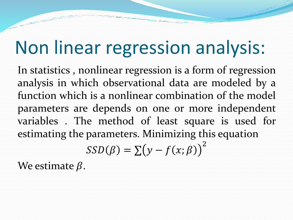
Non linear regression analysis:In statistics , nonlinear regression is a form of regressionanalysis in which observational data are modeled by afunction which is a nonlinear combination of the modelparameters are depends on one or more independentvariables . The method of least square is used forestimating the parameters. Minimizing this equation

𝑆𝑆𝐷 𝛽 = ∑ 𝑦 − 𝑓 𝑥; 𝛽2

We estimate 𝛽.

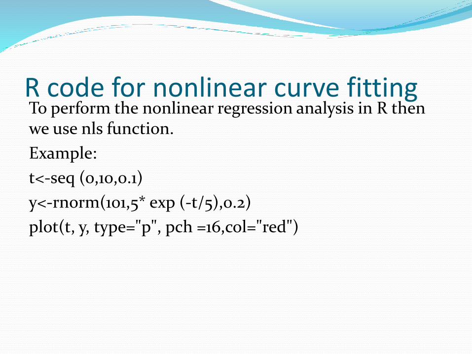
R code for nonlinear curve fittingTo perform the nonlinear regression analysis in R then we use nls function.

Example:

t<-seq (0,10,0.1)

y<-rnorm(101,5* exp (-t/5),0.2)

plot(t, y, type="p", pch =16,col="red")

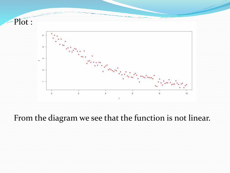
Plot :

From the diagram we see that the function is not linear.

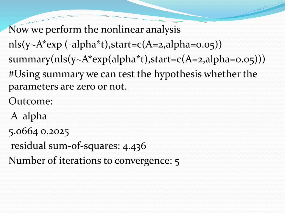
Now we perform the nonlinear analysis

nls(y~A*exp (-alpha*t),start=c(A=2,alpha=0.05))

summary(nls(y~A*exp(alpha*t),start=c(A=2,alpha=0.05)))

#Using summary we can test the hypothesis whether the parameters are zero or not.

Outcome:

A alpha

5.0664 0.2025

residual sum-of-squares: 4.436

Number of iterations to convergence: 5

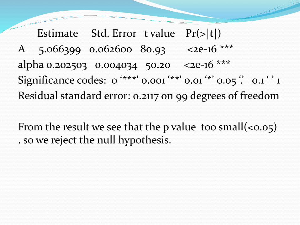
Estimate Std. Error t value Pr(>|t|)

A 5.066399 0.062600 80.93 <2e-16 ***

alpha 0.202503 0.004034 50.20 <2e-16 ***

Significance codes: 0 ‘***’ 0.001 ‘**’ 0.01 ‘*’ 0.05 ‘.’ 0.1 ‘ ’ 1

Residual standard error: 0.2117 on 99 degrees of freedom

From the result we see that the p value too small(<0.05) . so we reject the null hypothesis.

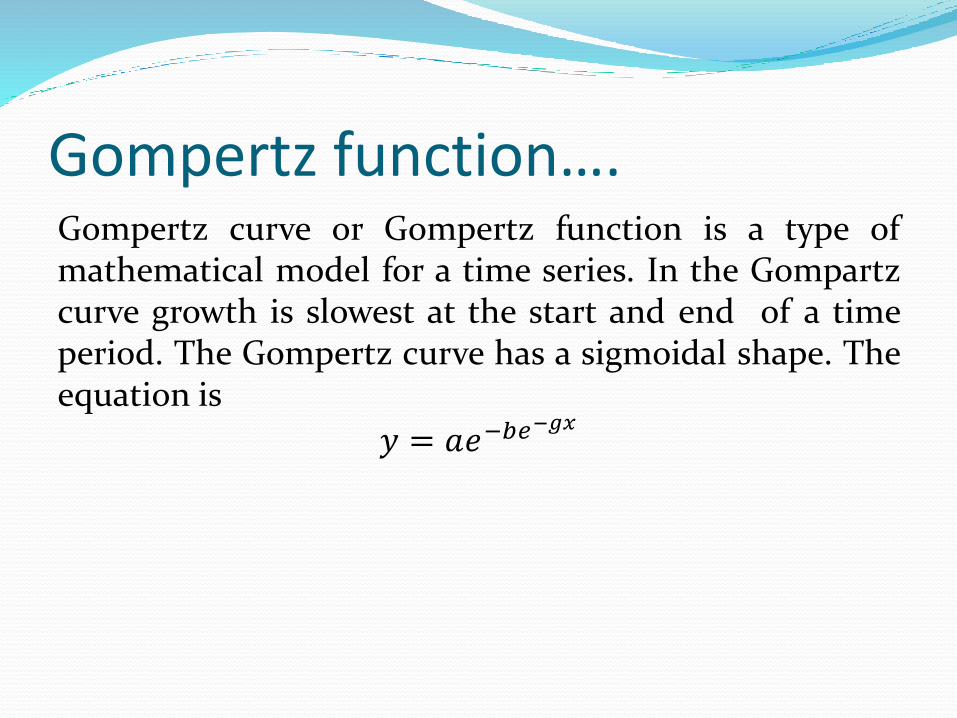
Gompertz function….Gompertz curve or Gompertz function is a type ofmathematical model for a time series. In the Gompartzcurve growth is slowest at the start and end of a timeperiod. The Gompertz curve has a sigmoidal shape. Theequation is

𝑦 = 𝑎𝑒−𝑏𝑒−𝑔𝑥

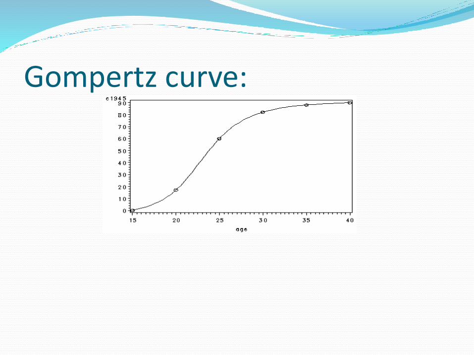
Gompertz curve:

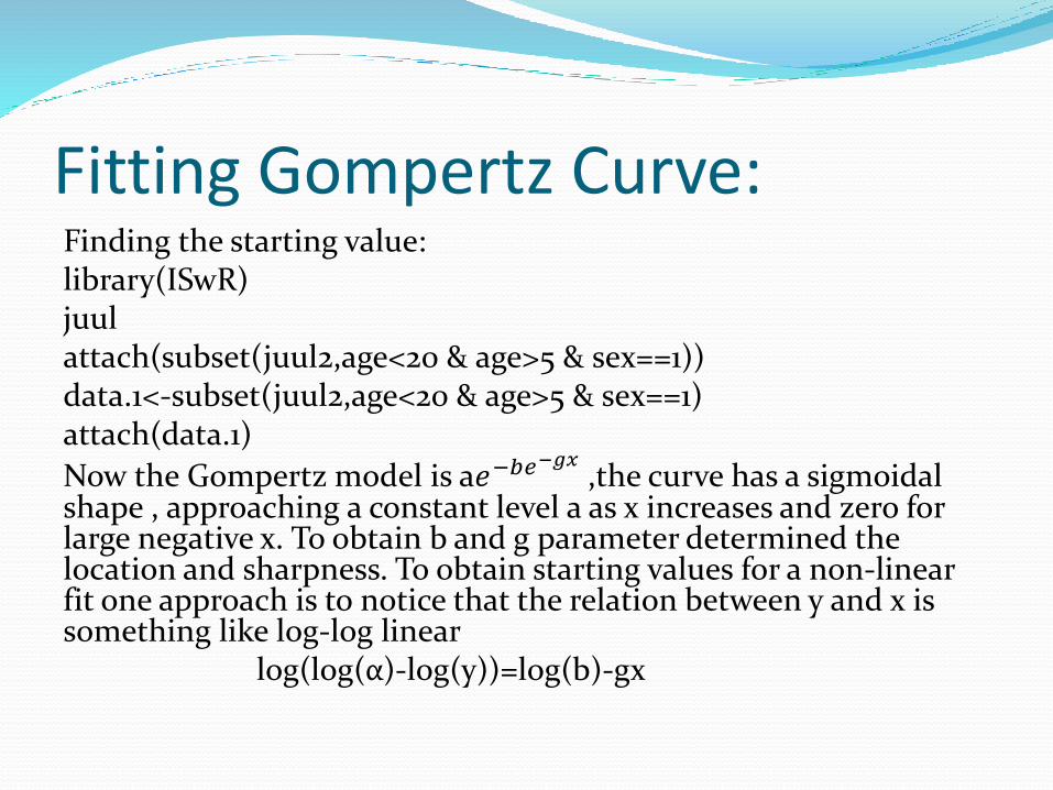
Fitting Gompertz Curve:Finding the starting value:library(ISwR)juulattach(subset(juul2,age<20 & age>5 & sex==1))data.1<-subset(juul2,age<20 & age>5 & sex==1)attach(data.1)

Now the Gompertz model is a𝑒−𝑏𝑒−𝑔𝑥

,the curve has a sigmoidal shape , approaching a constant level a as x increases and zero for large negative x. To obtain b and g parameter determined the location and sharpness. To obtain starting values for a non-linear fit one approach is to notice that the relation between y and x is something like log-log linear

log(log(α)-log(y))=log(b)-gx

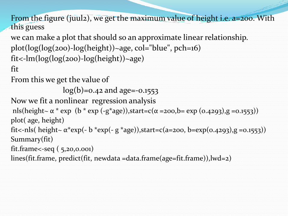
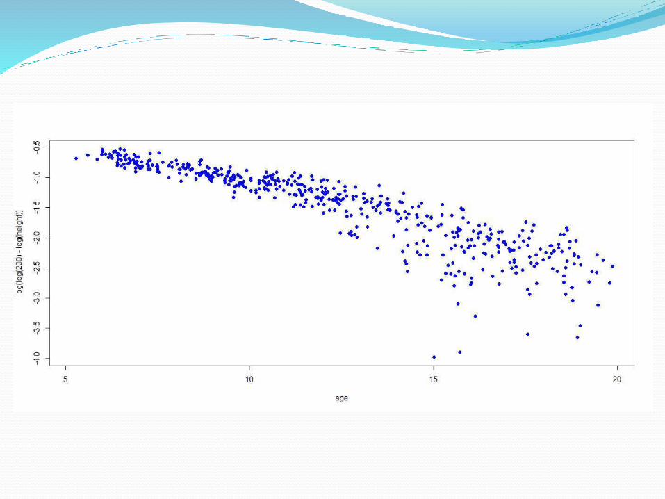
From the figure (juul2), we get the maximum value of height i.e. a=200. With this guess

we can make a plot that should so an approximate linear relationship.

plot(log(log(200)-log(height))~age, col="blue", pch=16)

fit<-lm(log(log(200)-log(height))~age)

fit

From this we get the value of

log(b)=0.42 and age=-0.1553

Now we fit a nonlinear regression analysisnls(height~ α * exp (b * exp (-g*age)),start=c(α =200,b= exp (0.4293),g =0.1553))

plot( age, height)

fit<-nls( height~ α*exp(- b *exp(- g *age)),start=c(a=200, b=exp(0.4293),g =0.1553))

Summary(fit)

fit.frame<-seq ( 5,20,0.001)

lines(fit.frame, predict(fit, newdata =data.frame(age=fit.frame)),lwd=2)

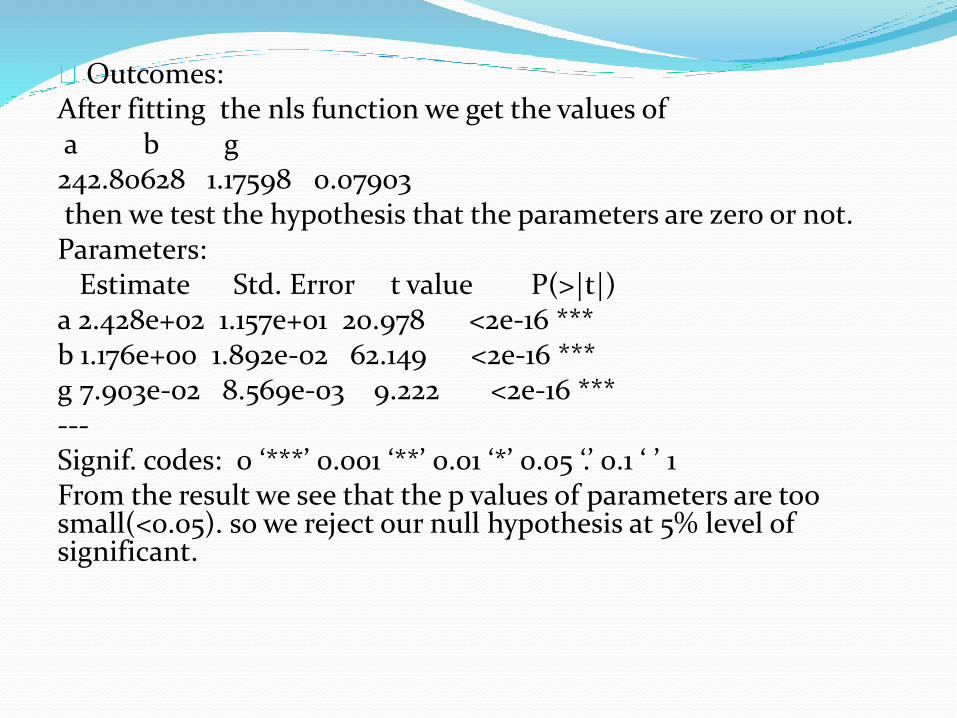
Outcomes:After fitting the nls function we get the values ofa b g 242.80628 1.17598 0.07903 then we test the hypothesis that the parameters are zero or not.Parameters:

Estimate Std. Error t value P(>|t|) a 2.428e+02 1.157e+01 20.978 <2e-16 ***b 1.176e+00 1.892e-02 62.149 <2e-16 ***g 7.903e-02 8.569e-03 9.222 <2e-16 ***---Signif. codes: 0 ‘***’ 0.001 ‘**’ 0.01 ‘*’ 0.05 ‘.’ 0.1 ‘ ’ 1From the result we see that the p values of parameters are too small(<0.05). so we reject our null hypothesis at 5% level of significant.

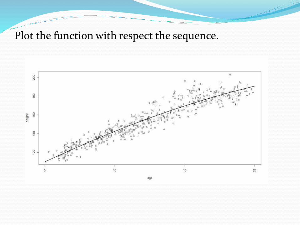
Plot the function with respect the sequence.

Self starting models:

Doesn't need to input initial values.

This type of functions are starting with SS in R

Ssgompertz.

library(ISwR)

age.height<-subset(juul2,age<20 & age>5 & sex==1)

attach(age.height)

nls(height~ SSgompertz(age,α,b, g ))

α b g

242.807 1.176 0.924

residual sum-of-squares: 23151

Draw back of self starting method:One minor drawback of self starting models is that we can not just transform them if you want to see if the model fits better on, e.g. a log-transformation

nls(log(height)~log(SSgompertz(age,α,b,g)))

So we can not use any transformation in self starting model.

Thank you……