non-linear compartmental systems: extensions of s.r. bernard's urn model
TRANSCRIPT
Bulletin ofMathemoticolBiolo~ Vol. 47. No. 2, pp. 19’3-204.1985. Printed in Great Britain
00Y2-8240/85$3.00+0.00 Pergamon Press Ltd.
0 1 Y85 Society for Mathematical Biology
NON-LINEAR COMPARTMENTAL SYSTEMS: EXTENSIONS OF S. R. BERNARD’S URN MODEL*
n MARY G. LEITNAKER Department of Statistics, The University of Tennessee, Knoxville, TN 37996, U.S.A.
n PETER PURDUE Department of Statistics, University of Kentucky, Lexington, KY 40506, U.S.A.
One of the limitations of stochastic, linear compartmental systems is the small degree of variability in the contents of compartments. S. R. Bernard’s (1981) urn model (S. R. Bernard et al., Bulk math. Biol. 43, 3345.) which allows for bulk arrivals and departures from a one-compartment system, was suggested as a way of increasing content variability. In this paper, we show how the probability distribution of the contents of an urn model may be simply derived by studying an appropriate set of exchangeable random variables. In addition, we show how further increases in variability may be modeled by allowing the size of arrivals and departures to be random.
1. Introduction. Stochastic compartmental models have typically been
constructed by describing the movement of a singli: particle through a com- partmental system. Thakur et al. (1972) consider a one-compartment system
where movement through the compartment is described by:
PAt + o(At) = P{a given particle departs in (t, t + At)}, p > 0 (1)
f(t) At + o( At) = P{a given particle enters in (t, t + At)}, f(t) > 0.
Purdue (1974) considers a more general system for which entry to the process is described by a nonhomogeneous Poisson Process with parameter m(t) and the departure process by a general distribution F(x, t), where 1 - F(x, t) is the probability that a particle which enters at time x > 0 is present in the compartment at time t.
One of the consequences of modeling a one-compartment system by considering the behavior of single particles is the small degree of variability present in the model when modeling the movement of a large number of particles. In the models considered by Thakur and Purdue, the coefficient
* Supported by NSF Grant No. MCS 81022501.
193
194 M. G. LEITNAKER AND P. PURDUE
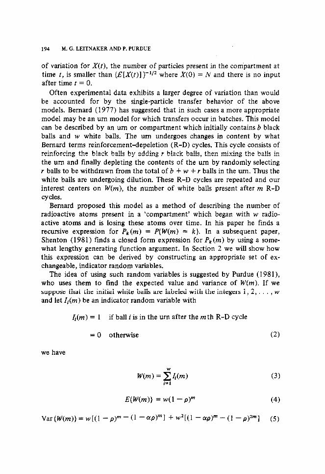
of variation for X(t), the number of particles present in the compartment at time t, is smaller than {E[X(t)] }-i/* where X(0) = N and there is no input after time C = 0.
Often experimental data exhibits a larger degree of variation than would be accounted for by the single-particle transfer behavior of the above models. Bernard (1977) has suggested that in such cases a more appropriate model may be an urn model for which transfers occur in batches. This model can be described by an urn or compartment which initially contains b black balls and w white balls. The urn undergoes changes in content by what Bernard terms reinforcement-depeletion (R-D) cycles. This cycle consists of reinforcing the black balls by adding r black balls, then mixing the balls in the urn and finally depleting the contents of the urn by randomly selecting r balls to be withdrawn from the total of b + w + r balls in the urn. Thus the white balls are undergoing dilution. These R-D cycles are repeated and our interest centers on W(m), the number of white balls present after m R-D cycles.
Bernard proposed this model as a method of describing the number of radioactive atoms present in a ‘compartment’ which began with w radio- active atoms and is losing these atoms over time. In his paper he finds a recursive expression for Pk(m) = P{W(m) = k}. In a subsequent paper, Shenton (1981) finds a closed form expression for Pk(m) by using a some- what lengthy generating function argument. In Section 2 we will show how this expression can be derived by constructing an appropriate set of ex- changeable, indicator random variables.
The idea of using such random variables is suggested by Purdue (1981), who uses them to find the expected value and variance of W(m). If we suppose that the initial white balls are iabeled with the integers 1, 2, . . . , w
and let Ii(in) be an indicator random variable with
IrW = 1 if bail i is in the urn after the m th R-D cycle
we have
= 0 otherwise
W(m) = &d i=l
(2)
(3)
E(W(m)} = w( 1 - p)” (4)
Var{W(m)}= w[(l -p)“-(1 -WY1 + W*[(l -WY-(1 -p>*“] (5)
NON-LINEARCOMPARTMENTALSYSTEMS 195
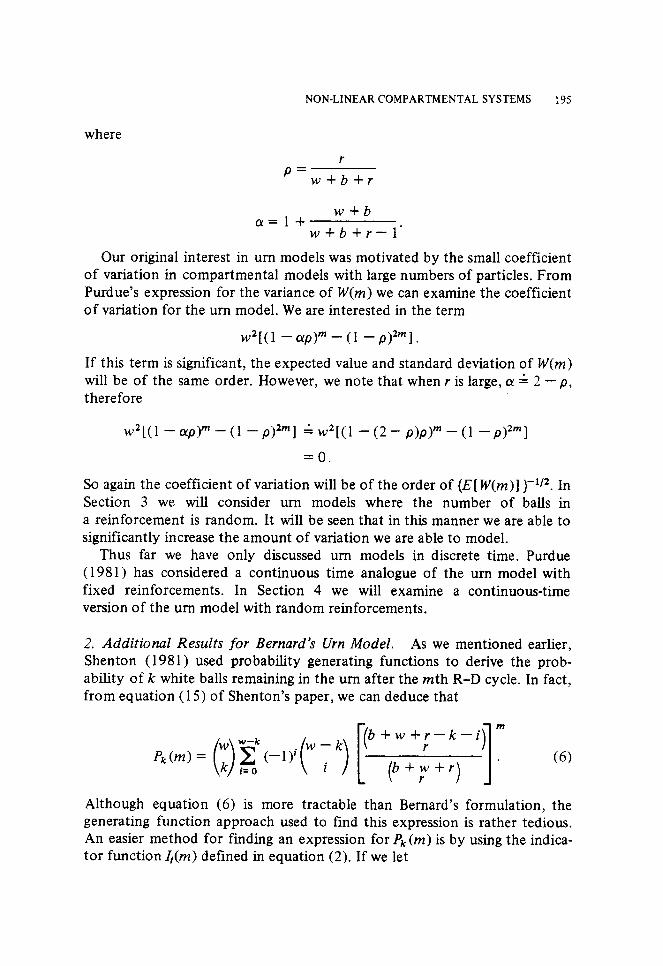
where
r P=
w+b+r
CY=1+ w+b
w+b+r-1’
Our original interest in urn models was motivated by the small coefficient of variation in compartmental models with large numbers of particles. From Purdue’s expression for the variance of W(m) we can examine the coefficient of variation for the urn model. We are interested in the term
WQl -spy-((1 -p)y
If this term is significant, the expected value and standard deviation of W(m) will be of the same order. However, we note that when r is large, 01 A 2 -p, therefore
= 0.
So again the coefficient of variation will be of the order of {E[ W(m)] }-l/2. In Section 3 we will consider urn models where the number of balls in a reinforcement is random. It will be seen that in this manner we are able to significantly increase the amount of variation we are able to model.
Thus far we have only discussed urn models in discrete time. Purdue (1981) has considered a continuous time analogue of the urn model with fixed reinforcements. In Section 4 we will examine a continuous-time version of the urn model with random reinforcements.
2. Additional Results for Bernard’s Urn Model. As we mentioned earlier, Shenton (1981) used probability generating functions to derive the prob- ability of k white balls remaining in the urn after the mth R-D cycle. In fact, from equation (15) of Shenton’s paper, we can deduce that
Although equation (6) is more tractable than Bernard’s formulation, the generating function approach used to find this expression is rather tedious. An easier method for finding an expression for P,(m) is by using the indica- tor function Ii(m) defined in equation (2). If we let
196 M. G. LEITNAKER AND P. PURDUE
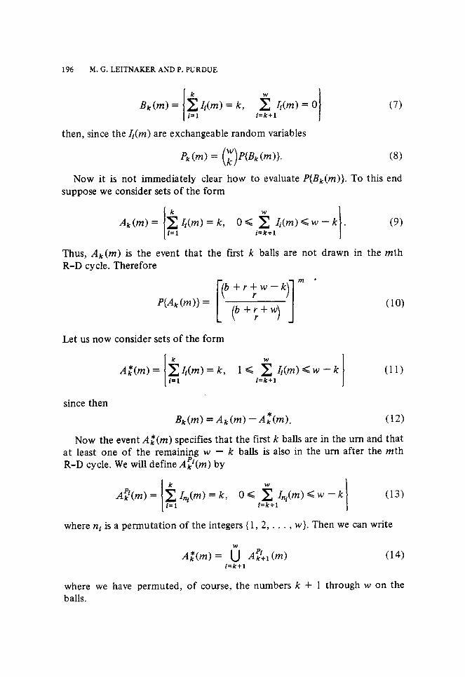
Bk(rn) = 5 I;:(m) = k, I g Ij(m) = 0 i=1 i=k+l
then, since the 4(m) are exchangeable random variables
(7)
Now it is not immediately clear how to evaluate P{B&)}. To this end suppose we consider sets of the form
&(m)= I &(m)=k, 09 2 h(m)<W--k . I (9) i=1 i=k+l
Thus, Ak(m) is the event that the first k balls are not drawn in the mth R-D cycle. Therefore
Let us now consider sets of the form
(10)
G(m)= &Fl)=k, l< E h(m)<w--k I I
(11) i=l i=k+l
since then
Bkh) = Akb> -‘d(m). (12)
Now the event A;(m) specifies that the first k balls are in the urn and that at least one of the remaining w - k balls is also in the urn after the mth R-D cycle. We will define A;(m) by
A&z) = i Inl(m) = k, I OG 5 I,&m)Gw-k I (13) f=l i=k+l
where nf is a permutation of the integers { 1, 2, . . . , w}. Then we can write
i=k+l
(14)
where we have permuted, of course, the numbers k + 1 through w on the balls.
NON-LINEARCOMPARTMENTALSYSTEMS 197
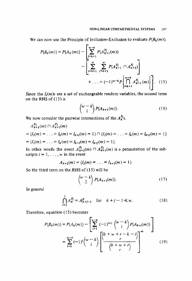
We can now use the Principle of Inclusion-Exclusion to evaluate P{&(m)}.
P{Bk(m)) = P{Ak(m)) -
[ i=k+l
+ . . . + (-lykP “ri” A?+, (m) I i=k+ 1
. II (15)
Since the h(m)s are a set of exchangeable random variables, the second term ontheRHSof(15)is
(16)
We now consider the pairwise intersections of the A;s.
pi A,+l(m) nAk+l(m) PI
= {In = . . . = &(m) = &+i(m) = 1 } n {I&m) = . . . = &(m) = &+,(m) = 1 }
= {Il(rn) = . . . = &(m) = &+f(m) = I&,(m) = 1).
In other words the event A;+l(m) f7 Aii’,l(m) is a permutation of the sub- scripts i = 1, . . . , w in the event
Ak+&Z) = {Ii(m) = . . . = Ik+z(m) = I}.
So the third term on the.RHS of (15) will be
( ) w ; k P{&+,(m)). (17)
In general
h A? = Af+,-1 for k+j -1Gw. (18) i=1
Therefore, equation (15) becomes
(19)
198 M.G.LEITNAKERANDP.PURDUE
and
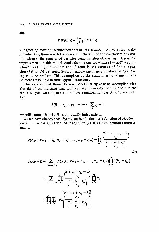
3. Effect of. Random Reinforcements in Urn Models. As we noted in the Introduction, there was little increase in the size of the coefficient of varia- tion when r, the number of particles being transferred, was large. A possible improvement on this model would then be one for which (1 - ap)” was not ‘close’ to (1 - P)~” so that the w2 term in the variance of W(m) [equa- tion (S)] would be larger. Such an improvement may be observed by allow- ing r to be random. This assumption of the randomness of r might even be more reasonable in some applied situations.
This extension of Bernard’s urn model is fairly easy to accomplish with the aid of the indicator functions we have previously used. Suppose at the ith R-D cycle we add, mix and remove a random number, Riy of black balls. Let
PUG = ‘I)= ~j where zpj = 1. i
We will assume that the Ris are mutually independent. As we have already seen, &(m) can be obtained as a function of P{Aj(m)},
j=k,..., w for Al(m) defined in equation (9). If we have random reinforce- ments:
P(& (m>/R 1 = rjl, R2 = rj2, . . . , R, = rjm} = fi >
S=l
(20)
fb + w + q, - k\
I-I&S s=l
NON-LINEAR COMPARTMENTAL SYSTEMS 199
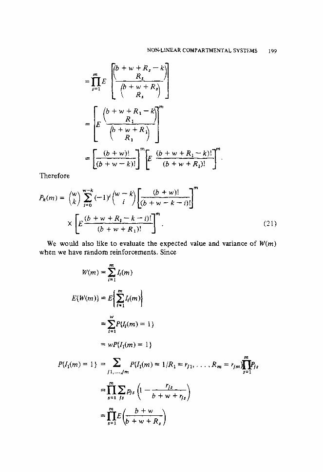
Therefore
m 1
(21)
We would also like to evaluate the expected value and variance of W(m) when we have random reinforcements. Since
W(m) =&n) i=l
= wP{ll(m) = 1)
P{ll(m) = l} = 2 P{ll(m) = l/R, = rll, . . . , R, = rf,,&8’js iL...,lm s=l
m
“(
b+w = s=lE b + w + R,
200 M.G.LEITNAKERANDP.PURDUE
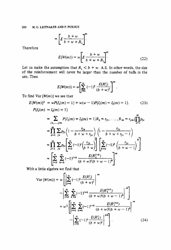
Therefore
E{W(m)}=w Eb,":=, I m
1
. 1
(22)
Let us make the assumption that RI < b + w. A.S. In other words, the size of the reinforcement will never be larger than the number of balls in the urn. Then
E(R’,) m (-l)i(b +w)i 1 -
To find Var {W(m)} we see that
EMN2 = wP{l&m) = l} + w(w - l)P(l,(m) = 12(m) = l}.
P{1@) = I*(m) = 1 }
(23)
= c P(J,(m)=f,(m)= l~R~=r,,,...,R,=rjm)llfIpi, /l,...,/m S=l
With a little algebra we find that
Var{ W(m)}=
(24)
NON-LINEARCOMPARTMENTAL SYSTEMS 201
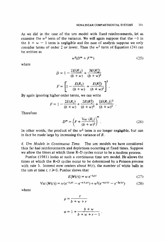
As we did in the case of the urn model with fixed reinforcements, let us examine the w* term of the variance. We will again suppose that the -1 in the b + w - 1 term is negligible and for ease of analysis suppose we only consider terms of order 2 or lower. Then the w* term of Equation (24) can be written as
where
w*(D* + F”) (25)
D = 1 2J5(Ri.) + 3E(R:)
(b +w) (b +w)2
E(R,) E(R:) 2
(b + w) + (b + w)* 1 . By again ignoring higher order terms, we can write
Therefore
In other words, the product of the w* term is no longer negligible, but can in fact be made large by increasing the variance of R.
4. Urn Models in Continuous Time. The urn models we have considered thus far had reinforcements and depletions occurring at fixed times. Suppose we allow the times at which these R-D cycles occur to be a random process.
Purdue (198 1) looks at such a continuous time urn model. He allows the times at which the R-D cycles occur to be determined by a Poisson process with rate h. Interest now centers about W(t), the number of white balls in the urn at time t, t 2 0. Purdue shows that
E{W(t)) = w emapr (27)
Var {w(t)} = w(e-hQr - e-ahPr) + W*(e-Wht - e-*Phr) (38)
where
p= r b+w+r
cr=1+ b+w
b+w+r-1’
202 M. G. LEITNAKER AND P. PURDUE
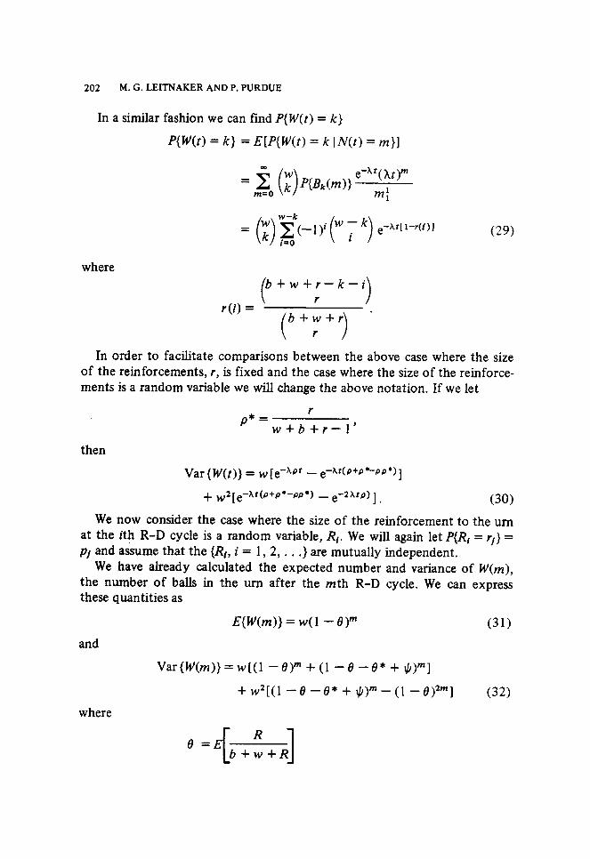
In a similar fashion we can find P(IV(t) = k}
P{W(t) = k} = E[P{W(t) = k I N(t) = m}]
0
= x0 e-Af(Xt)m
m=O ; P{Bk(m)) m:
(29)
where
In order to facilitate comparisons between the above case where the size of the reinforcements, r, is fixed and the case where the size of the reinforce- ments is a random variable we will change the above notation. If we let
then
p* = r
w+b+r-1’
Var{W(t)} = w[e-hQr - e-At(O+O*-PP*)]
+ W2[e-hr(o+~*-bw*) - e_2AtP)]. (30)
We now consider the case where the size of the reinforcement to the urn at the ith R-D cycle is a random variable, R,. We will again let P{R, = r,} = pf and assume that the {Rt, i = 1,2, . . .} are mutually independent.
We have already calculated the expected number and variance of W(m), the number of balls in the urn after the mth R-D cycle. We can express these quantities as
and
E{W(m)} = w( 1 - O>m (31)
+ w2[(1 -e-e* + J/)“-(l-e)2”] (32)
where
8 =E R
[ 1 b+w+R
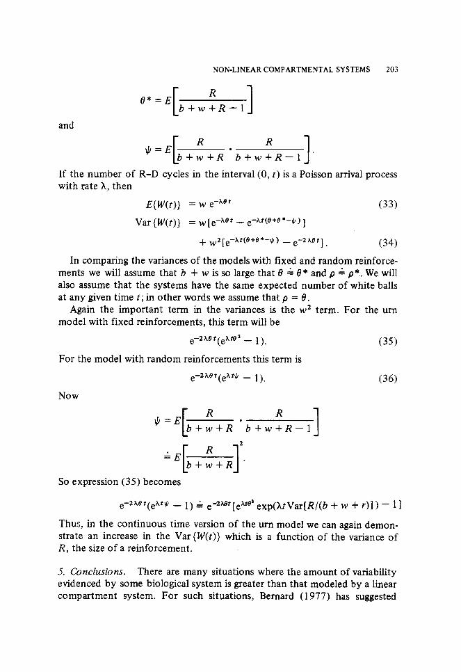
NON-LINEARCOMPARTMENTALSYSTEMS 203
e*=E R
b+w+R-1 I
and
R
‘b+w+R-1 ’ I
If the number of R-D cycles in the interval (0, t) is a Poisson arrival process with rate A, then
E{W(t)} = w emher (33)
Var{W(t)} = w[e-het - e-hr(e+e’-JI) ]
+ W2[e-ht(e+e*-$) _ e-2het] (34)
In comparing the variances of the models with fixed and random reinforce- ments we will assume that b + w is so large that 8 A 0 * and p G p*.. We will also assume that the systems have the same expected number of white balls at any given time t; in other words we assume that p = 8.
Again the important term in the variances is the w2 term. For the urn model with fixed reinforcements, this term will be
e-2het (e hte2 _ 1)
For the model with random reinforcements this term is
(35)
e-2her(ehW - 1). (36)
Now
R
‘b+w+R-1 1 AE R ’ [ 1 b+w+R .
So expression (35) becomes
e-2het(ehtiL _ 1) ; e-2h8t Lexte2 exp(htVar[R/(b + w + r)l) - 11
Thus, in the continuous time version of the urn model we can again demon- strate an increase in the Var {w(t)} which is a function of the variance of R, the size of a reinforcement.
5. Conclusions. There are many situations where the amount of variability evidenced by some biological system is greater than that modeled by a linear compartment system. For such situations, Bernard (1977) has suggested
204 M.G.LEITNAKERANDP.PURDUE
using an urn model. Here we have shown how the distribution of the contents of such an urn model may be found by the definition of an appropriate set of exchangeable random variables. This approach is felt to be simpler than the generating function technique used by Shenton (198 1) and thus can be more easily generalized. We then use this approach to extend the results for Bernard’s model. By allowing the size of reinforcements to the urn model to be random, we note an increase in the variability of the contents of the urn both in the discrete time model of Bernard and the continuous time model developed by Purdue (198 1).
LITERATURE
Bernard, S. R. 1977. “An Urn Model Study of Variability Within a Compartment.” Bull. math. Biol. 39,463-470.
-, M. Sobel and V. R. R. Uppuluri. 198 1. “On a Two Urn Model of Polya-type.” Bul!. math. Biol, 43, 33-45.
Purdue, P. 1974. “Stochastic Theory of Compartments: One and Two Compartment Systems.” BulL math. BioL 36, 577-587.
-. 1981. “Variability in a Single Compartment System: A Note on S. R. Bernard’s Model.” Bull. math. BioL 43, 11 l-l 16.
Shenton, L. R. 1981. “A Reinforcement-Depletion Urn Problem-I. Basic Theory.” Bull. math. Biol. 43, 327-340.
Thakur, A. K., A. Rescigno and D. E. Schafer. 1972. “On the Stochastic Theory of Compartments: A Single Compartment System.” Bull. math. Biophys. 35,53-65.
RECEIVED 6-29-84 REVISED 10-16-84