nobs linear algebra and vector geometry - jeffw.xyz · in linear algebra, we start with linear...
TRANSCRIPT
NoBS Linear Algebraand Vector Geometry
Jeffrey Wang
January 29, 2018 – May 20, 2018version 2018.05.20.18:56
First edition

ii

Contents
Author’s Notes i0.1 NoBS . . . . . . . . . . . . . . . . . . . . . . . . . . . . . . . . . . . . . . . . . . . . . i0.2 What NoBS Linear Algebra covers . . . . . . . . . . . . . . . . . . . . . . . . . . . . i0.3 What this study guide does . . . . . . . . . . . . . . . . . . . . . . . . . . . . . . . . i0.4 What this study guide does not do . . . . . . . . . . . . . . . . . . . . . . . . . . . . i0.5 Other study resources . . . . . . . . . . . . . . . . . . . . . . . . . . . . . . . . . . . i0.6 Dedication . . . . . . . . . . . . . . . . . . . . . . . . . . . . . . . . . . . . . . . . . . i0.7 Sources . . . . . . . . . . . . . . . . . . . . . . . . . . . . . . . . . . . . . . . . . . . . ii0.8 Copyright and resale . . . . . . . . . . . . . . . . . . . . . . . . . . . . . . . . . . . . ii
1 Systems of linear equations 11.1 Introduction . . . . . . . . . . . . . . . . . . . . . . . . . . . . . . . . . . . . . . . . . 11.2 Matrices . . . . . . . . . . . . . . . . . . . . . . . . . . . . . . . . . . . . . . . . . . . 2
Matrix notation . . . . . . . . . . . . . . . . . . . . . . . . . . . . . . . . . . . . . . . 2Solving matrices . . . . . . . . . . . . . . . . . . . . . . . . . . . . . . . . . . . . . . . 3Existence and uniqueness (part 1) . . . . . . . . . . . . . . . . . . . . . . . . . . . . . 3Row reduction and echelon form . . . . . . . . . . . . . . . . . . . . . . . . . . . . . 4Evaluating solutions of a linear system . . . . . . . . . . . . . . . . . . . . . . . . . . 5Existence and uniqueness (part 2) of matrices . . . . . . . . . . . . . . . . . . . . . . 6
1.3 Vectors and vector equations . . . . . . . . . . . . . . . . . . . . . . . . . . . . . . . 6Vector operations . . . . . . . . . . . . . . . . . . . . . . . . . . . . . . . . . . . . . . 6Vectors and matrices . . . . . . . . . . . . . . . . . . . . . . . . . . . . . . . . . . . . 7Combining vectors . . . . . . . . . . . . . . . . . . . . . . . . . . . . . . . . . . . . . 7
1.4 Linear combinations . . . . . . . . . . . . . . . . . . . . . . . . . . . . . . . . . . . . 7Span . . . . . . . . . . . . . . . . . . . . . . . . . . . . . . . . . . . . . . . . . . . . . 8Existence and uniqueness (part 3) of linear combinations . . . . . . . . . . . . . . . 8
1.5 Basic matrix multiplication . . . . . . . . . . . . . . . . . . . . . . . . . . . . . . . . . 101.6 The matrix equation A~x = ~b . . . . . . . . . . . . . . . . . . . . . . . . . . . . . . . . 11
Existence and uniqueness (part 4): Four ways to represent a consistent linear system 111.7 Homogeneous linear systems . . . . . . . . . . . . . . . . . . . . . . . . . . . . . . . 12
Parametric vector form . . . . . . . . . . . . . . . . . . . . . . . . . . . . . . . . . . . 12Non-homogeneous linear systems in terms of homogeneous linear systems . . . . 13
1.8 Linear independence . . . . . . . . . . . . . . . . . . . . . . . . . . . . . . . . . . . . 13Linear independence of a set of one vector . . . . . . . . . . . . . . . . . . . . . . . . 13Linear independence of a set of two vectors . . . . . . . . . . . . . . . . . . . . . . . 14Linear independence of a set of multiple vectors . . . . . . . . . . . . . . . . . . . . 14
1.9 Linear transformations . . . . . . . . . . . . . . . . . . . . . . . . . . . . . . . . . . . 14
iii
iv CONTENTS
Properties of linear transformations . . . . . . . . . . . . . . . . . . . . . . . . . . . 151.10 The matrix of a linear transformation . . . . . . . . . . . . . . . . . . . . . . . . . . . 16
Geometric transformations in R2 . . . . . . . . . . . . . . . . . . . . . . . . . . . . . 16Another vector representation format . . . . . . . . . . . . . . . . . . . . . . . . . . 16Existence and uniqueness (part 5): Onto and one-to-one . . . . . . . . . . . . . . . . 17
1.11 Summary of Chapter 1: Ways to represent existence and uniqueness . . . . . . . . 18
2 Matrix algebra 192.1 Matrix operations . . . . . . . . . . . . . . . . . . . . . . . . . . . . . . . . . . . . . . 19
Addition and scalar multiplication . . . . . . . . . . . . . . . . . . . . . . . . . . . . 19Matrix multiplication . . . . . . . . . . . . . . . . . . . . . . . . . . . . . . . . . . . . 20
2.2 Transpose and inverse matrices . . . . . . . . . . . . . . . . . . . . . . . . . . . . . . 22Transpose . . . . . . . . . . . . . . . . . . . . . . . . . . . . . . . . . . . . . . . . . . 22Inverse matrices . . . . . . . . . . . . . . . . . . . . . . . . . . . . . . . . . . . . . . . 23Inverse matrices and row equivalence . . . . . . . . . . . . . . . . . . . . . . . . . . 24
2.3 Characteristics of invertible matrices: the Invertible Matrix Theorem . . . . . . . . 25Invertible linear transformations . . . . . . . . . . . . . . . . . . . . . . . . . . . . . 26
2.4 Partitioned matrices . . . . . . . . . . . . . . . . . . . . . . . . . . . . . . . . . . . . . 262.5 Subspaces . . . . . . . . . . . . . . . . . . . . . . . . . . . . . . . . . . . . . . . . . . 26
Column space . . . . . . . . . . . . . . . . . . . . . . . . . . . . . . . . . . . . . . . . 27Null space . . . . . . . . . . . . . . . . . . . . . . . . . . . . . . . . . . . . . . . . . . 27Relating column space and null space together . . . . . . . . . . . . . . . . . . . . . 28
2.6 Basis . . . . . . . . . . . . . . . . . . . . . . . . . . . . . . . . . . . . . . . . . . . . . 28Standard basis . . . . . . . . . . . . . . . . . . . . . . . . . . . . . . . . . . . . . . . . 29Nonstandard basis . . . . . . . . . . . . . . . . . . . . . . . . . . . . . . . . . . . . . 29Basis examples . . . . . . . . . . . . . . . . . . . . . . . . . . . . . . . . . . . . . . . . 29
2.7 Coordinate vector . . . . . . . . . . . . . . . . . . . . . . . . . . . . . . . . . . . . . . 312.8 Dimension, rank, and nullity . . . . . . . . . . . . . . . . . . . . . . . . . . . . . . . 31
3 Determinants 333.1 Introduction to determinants . . . . . . . . . . . . . . . . . . . . . . . . . . . . . . . 33
Pre-definition notations and conventions . . . . . . . . . . . . . . . . . . . . . . . . 33Definition of the determinant . . . . . . . . . . . . . . . . . . . . . . . . . . . . . . . 34Laplace expansion (cofactor expansion) . . . . . . . . . . . . . . . . . . . . . . . . . 34Sign patterns for terms of a determinant summation . . . . . . . . . . . . . . . . . . 34Triangular matrix determinant calculation . . . . . . . . . . . . . . . . . . . . . . . . 35
3.2 Properties of determinants . . . . . . . . . . . . . . . . . . . . . . . . . . . . . . . . . 35Summary of determinant properties . . . . . . . . . . . . . . . . . . . . . . . . . . . 36
3.3 Cramer’s rule . . . . . . . . . . . . . . . . . . . . . . . . . . . . . . . . . . . . . . . . 36
4 Vector spaces 374.1 Introduction to vector spaces and their relation to subspaces . . . . . . . . . . . . . 37
Subspaces in relation to vector spaces . . . . . . . . . . . . . . . . . . . . . . . . . . 384.2 Null spaces, column spaces, and linear transformations . . . . . . . . . . . . . . . . 394.3 Spanning sets . . . . . . . . . . . . . . . . . . . . . . . . . . . . . . . . . . . . . . . . 404.4 Coordinate systems . . . . . . . . . . . . . . . . . . . . . . . . . . . . . . . . . . . . . 404.5 Dimension of a vector space . . . . . . . . . . . . . . . . . . . . . . . . . . . . . . . . 414.6 Rank of a vector space’s matrix . . . . . . . . . . . . . . . . . . . . . . . . . . . . . . 42

CONTENTS v
4.7 Change of basis . . . . . . . . . . . . . . . . . . . . . . . . . . . . . . . . . . . . . . . 43Change of basis and the standard basis . . . . . . . . . . . . . . . . . . . . . . . . . . 43Finding the change of coordinates matrix . . . . . . . . . . . . . . . . . . . . . . . . 44
5 Eigenvalues and eigenvectors 455.1 Introduction to eigenvalues and eigenvectors . . . . . . . . . . . . . . . . . . . . . . 455.2 The characteristic equation: finding eigenvalues . . . . . . . . . . . . . . . . . . . . 47
Problem-solving process for triangular matrices . . . . . . . . . . . . . . . . . . . . 47Problem-solving process for general matrices . . . . . . . . . . . . . . . . . . . . . . 47
5.3 Similarity . . . . . . . . . . . . . . . . . . . . . . . . . . . . . . . . . . . . . . . . . . . 485.4 Diagonalization . . . . . . . . . . . . . . . . . . . . . . . . . . . . . . . . . . . . . . . 48
The process of diagonalizing matrices . . . . . . . . . . . . . . . . . . . . . . . . . . 49Example of diagonalizing a matrix . . . . . . . . . . . . . . . . . . . . . . . . . . . . 50
6 Orthogonality, least squares, and symmetry 516.1 Dot product, length, and distance . . . . . . . . . . . . . . . . . . . . . . . . . . . . . 51
Dot product/Inner product . . . . . . . . . . . . . . . . . . . . . . . . . . . . . . . . 51Length/magnitude of a vector . . . . . . . . . . . . . . . . . . . . . . . . . . . . . . 52Unit vector . . . . . . . . . . . . . . . . . . . . . . . . . . . . . . . . . . . . . . . . . . 52Distance between two vectors . . . . . . . . . . . . . . . . . . . . . . . . . . . . . . . 52
6.2 Introduction to orthogonality . . . . . . . . . . . . . . . . . . . . . . . . . . . . . . . 52Orthogonal vectors . . . . . . . . . . . . . . . . . . . . . . . . . . . . . . . . . . . . . 53Orthogonal complements . . . . . . . . . . . . . . . . . . . . . . . . . . . . . . . . . 53Orthogonal sets . . . . . . . . . . . . . . . . . . . . . . . . . . . . . . . . . . . . . . . 53Orthonormal sets . . . . . . . . . . . . . . . . . . . . . . . . . . . . . . . . . . . . . . 54Orthogonal projections onto lines . . . . . . . . . . . . . . . . . . . . . . . . . . . . . 54
6.3 Orthogonal projections onto subspaces . . . . . . . . . . . . . . . . . . . . . . . . . . 556.4 Gram–Schmidt process . . . . . . . . . . . . . . . . . . . . . . . . . . . . . . . . . . . 55
QR decomposition . . . . . . . . . . . . . . . . . . . . . . . . . . . . . . . . . . . . . 566.5 Symmetric matrices . . . . . . . . . . . . . . . . . . . . . . . . . . . . . . . . . . . . . 56
The Spectral Theorem . . . . . . . . . . . . . . . . . . . . . . . . . . . . . . . . . . . . 56Spectral decomposition . . . . . . . . . . . . . . . . . . . . . . . . . . . . . . . . . . . 56
7 Miscellaneous topics 577.1 Cross products . . . . . . . . . . . . . . . . . . . . . . . . . . . . . . . . . . . . . . . . 57

vi CONTENTS
Author’s Notes
0.1 NoBS
NoBS, short for ”no bull$#!%”, strives for succinct guides that use simple, smaller, relatableconcepts to develop a full understanding of overarching concepts.
0.2 What NoBS Linear Algebra covers
This guide succinctly and comprehensively covers most topics in an explanatory notes formatfor a college-level introductory Linear Algebra and Vector Geometry course.
0.3 What this study guide does
It explains all the concepts to you in an intuitive way so you understand the course materialbetter.
If you are a mathematics major, it is recommended you read a proof-based book.If you are not a mathematics major, this study guide is intended to make your life easier.
0.4 What this study guide does not do
This study guide is not intended as a replacement for a textbook. This study guide does notteach via proofs; rather, it teaches by concepts. If you are looking for a formalized, proof-basedtextbook, seek other sources.
0.5 Other study resources
NoBS Linear Algebra should by no means be your sole study material. For more conceptual,visual representations, 3Blue1Brown’s Essence of Linear Algebra video series on YouTube is highlyrecommended as a companion to supplement the information you learn from this guide.
Throughout this book, links to relevant Essence of Linear Algebra videos will be displayed foryou to watch.
0.6 Dedication
To all those that helped me in life: this is for you.
i
ii AUTHOR’S NOTES
Thank you to Edoardo Luna for introducing Essence of Linear Algebra to me. Without it, Iwould not have nearly as much intuitive understanding of linear algebra to write this guide.
0.7 Sources
This guide has been inspired by, and in some cases borrows, certain material from the followingsources, which are indicated below and will be referenced throughout this guide by parenthesesand their names when necessary:
• (Widmer) - Steven Widmer, University of North Texas, my professor from whom I tookthis course in Spring 2018.
• (Lay) - David C. Lay, Steven R. Lay, Judi J. McDonald, Linear Algebra and Its Applications(5th edition)
• Several concepts in Chapter 6 and 7 have text copied and modified from NoBS Calculuswritten by the same author as the author of NoBS Linear Algebra (Jeffrey Wang). For thisreason, no direct attribution is given inline, but instead given here.
• Some inline citations do not appear here but next to their borrowed content.
Note that this study guide is written along the progression of Linear Algebra and Its Applicationsby Lay, Lay, and McDonald (5th edition). However, Chapter 7 is a supplemental chapter thatdeviates from the progression of Lay and covers topics such as the cross product.
0.8 Copyright and resale
This study guide is free for use but copyright the author, except for sections borrowed from othersources. The PDF version of this study guide may not be resold under any circumstances. If youpaid for the PDF, request a refund from whomever sold it to you. The only acceptable sale ofthis study guide is for a physical copy as done so by the author or with his permission.
Chapter 1
Systems of linear equations
1.1 Introduction
In linear algebra, we start with linear equations. In high school algebra, we learned about thelinear equation y = mx + b. However, we will be considering linear equations with multiplevariables that are ordered, which can be written in the following form:
a1x1 + a2x2 + · · ·+ anxn = b
The coefficient may be any real number (a ∈ R). However, the variable must be to the 1 power.The following are linear equations:
• x1 = 5x2 + 7x3 − 12 – Nothing looks out of the ordinary here.
• x2 =√5(9− x3) + πx1 – The coefficients can be non-integers and irrational.
However, the following are NOT linear equations:
• 3(x1)2 + 5(x2) = 9 – We can’t have a quadratic.
• 9x1 + 7x2x3 = −45 – We also can’t have variables multiplying by each other.
• 3√x1+x2 = 2 – We furthermore can’t have roots of variables, nor any other non-polynomial
function.
• x3
x1+ x2 = 3 – Inverses are not allowed either.
• sinx1 + cos3 x2 − lnx3 + e−x4 = −9 – Obviously no transcendental functions are allowed.
A system of linear equations (or a linear system) is a collection of linear equations that sharethe same variables.
If an ordered list of values are substituted into their respective variables in the system ofequations and each equation of the system holds true, then we call this collection of values asolution.
Say we have the ordered list of values (1, 3, 2). This would be a solution of the followingsystem of linear equations:
x1 + x2 + x3 = 6x2 + x3 = 5
x3 = 2
1
2 CHAPTER 1. SYSTEMS OF LINEAR EQUATIONS
because if you substituted the solution for the respective variables, you get
1 + 3 + 2 = 63 + 2 = 5
2 = 2
which are all valid, true statements.A system can have more than one solution. We call the collection of all solutions the solution
set. If two systems have exactly the same solution set, they are actually the same system.In high school algebra, you learned that the solution of two linear equations was the point
at which they intersected; this still holds true, but in linear algebra, we’ll be dealing with moregeneralized cases that might be too complicated to solve graphically.
There are three possibilities (and only three) to the number of solutions a system can have: 0,1, and∞.
A system is inconsistent if it has no solutions and it is consistent if it has at least one solution.
• No solutions - inconsistent
• Exactly one solution - consistent
• Infinitely many solutions - consistent
1.2 Matrices
Matrix notation
An m × n matrix is a rectangular array (or, ordered listing) of numbers with m rows and ncolumns, where m and n are both natural numbers. We can use matrices to represent systems ina concise manner.
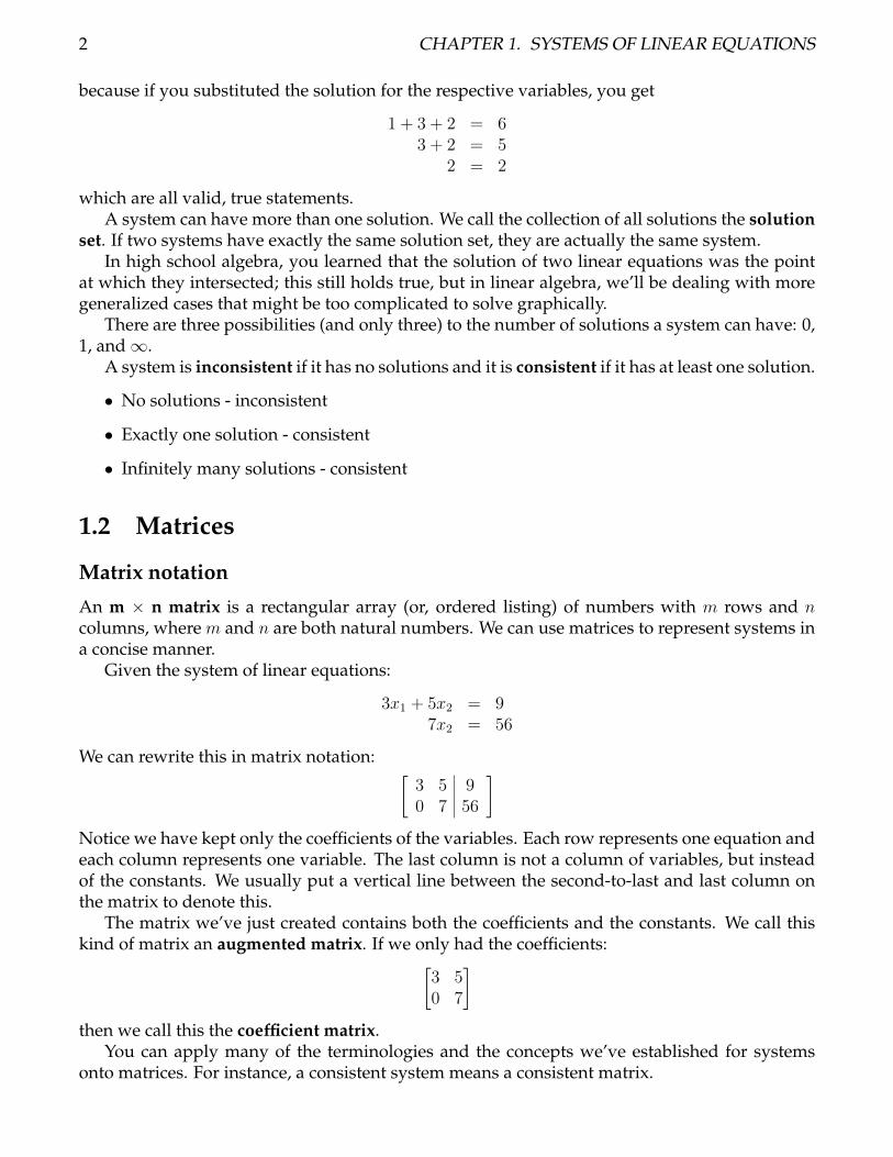
Given the system of linear equations:
3x1 + 5x2 = 97x2 = 56
We can rewrite this in matrix notation: [3 5 90 7 56
]Notice we have kept only the coefficients of the variables. Each row represents one equation andeach column represents one variable. The last column is not a column of variables, but insteadof the constants. We usually put a vertical line between the second-to-last and last column onthe matrix to denote this.
The matrix we’ve just created contains both the coefficients and the constants. We call thiskind of matrix an augmented matrix. If we only had the coefficients:[
3 50 7
]then we call this the coefficient matrix.
You can apply many of the terminologies and the concepts we’ve established for systemsonto matrices. For instance, a consistent system means a consistent matrix.
1.2. MATRICES 3
Solving matrices
We’re going to apply the same operations we used to solve systems of linear equations back inhigh school algebra, except this time in matrices.
The three elementary row operations for matrices are:
1. Scaling – multiplying all of the values on a row by a constant
2. Interchange – swapping the positions of two rows
3. Replacement – adding two rows together: the row that is being replaced, and a scaledversion of another row in the matrix.
These row operations are reversible. In other words, you can undo the effects of them laterin the process.
We consider two augmented matrices to be row equivalent if there is a sequence of elemen-tary row operations that can transform one matrix into another. Two matrices A and B mayappear different, but if you can go from matrix A to B using these elementary row operations,then A ∼ B. In fact, there are infinitely many row equivalent matrices.
Linking back to the previous section: if two augmented matrices are row equivalent, thenthey also have the same solution set, which again confirms that they are the same matrix/system.
Existence and uniqueness (part 1)
Two fundamental questions establish the status of a system/matrix:
1. Existence - does a solution exist? (i.e. Is this matrix consistent?)
2. Uniqueness - if a solution exists, is this solution unique?
The rest of this chapter is dedicated to the methods used to finding whether a solution existsand is unique. The first half focuses on concepts and techniques that give us existence, and thesecond half focuses on uniqueness. Then, we’ll combine them together in transformations.
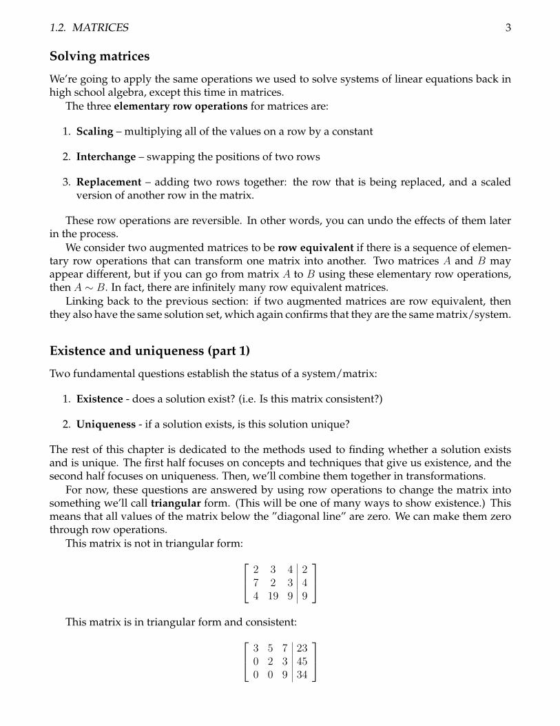
For now, these questions are answered by using row operations to change the matrix intosomething we’ll call triangular form. (This will be one of many ways to show existence.) Thismeans that all values of the matrix below the ”diagonal line” are zero. We can make them zerothrough row operations.
This matrix is not in triangular form: 2 3 4 27 2 3 44 19 9 9
This matrix is in triangular form and consistent: 3 5 7 23
0 2 3 450 0 9 34
4 CHAPTER 1. SYSTEMS OF LINEAR EQUATIONS
This matrix, while in triangular form, is NOT consistent: 7 8 9 100 11 8 50 0 0 3
This is because the last row says 0 = 3, which is false. Therefore, there are no solutions for thatmatrix, so therefore it is inconsistent.
Consistency = existence. They are the same thing.
Row reduction and echelon form
Now that we’re beginning to delve into solving matrices using row operations, let’s develop analgorithm and identify a pattern that will let us find the solution(s) of a matrix.
This pattern was identified in the previous section. We called it by an informal name (”trian-gular form”) but this is actually not its formal name. The pattern is called echelon form (or rowechelon form, pronounced ”esh-uh-lohn”). The official definition of echelon form is a matrixthat has the following properties:
1. Any rows of all zeros must be below any rows with nonzero numbers.
2. Each ”leading entry” of a row (which is the first nonzero entry, officially called a pivot) isin a column to the right of the leading entry/pivot of the row above it.
3. All entries in a column below a pivot must be zero.
While echelon form is helpful, we actually want to reduce a matrix down to reduced echelonform (or reduced row echelon form) to obtain the solutions of the matrix. There are two addi-tional requirements for a matrix to be in reduced echelon form:
4. The pivot in each nonzero row is 1. (All pivots in the matrix must be 1.)
5. Each pivot is the only nonzero entry of the column.
(Widmer)While there are infinitely many echelon forms for a certain matrix, there is only one unique
reduced echelon form for a certain matrix.Note that sometimes, reduced echelon form is not necessary to solve a problem in linear
algebra. Ask yourself if you really need reduced echelon form. Usually, the answer is no.A matrix in echelon form is an echelon matrix, and if in reduced echelon form, then it’s a
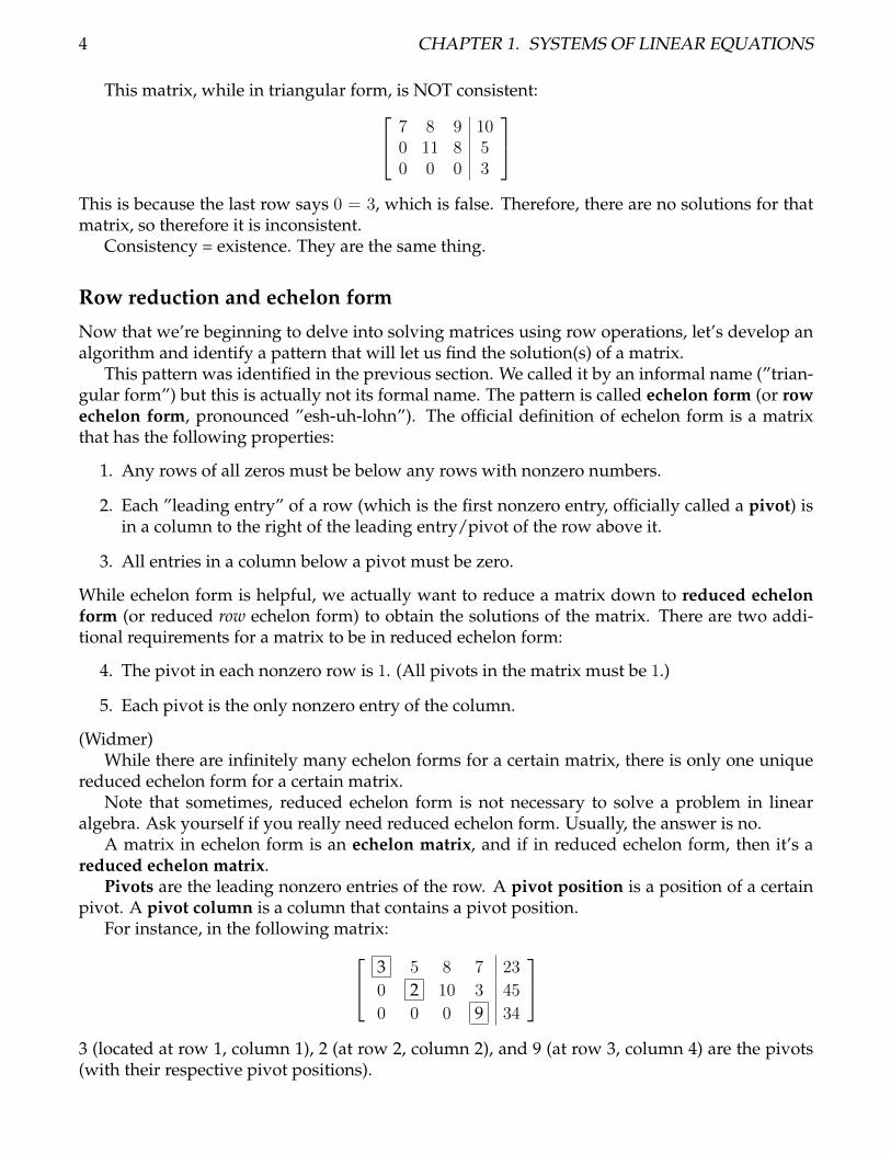
reduced echelon matrix.Pivots are the leading nonzero entries of the row. A pivot position is a position of a certain
pivot. A pivot column is a column that contains a pivot position.For instance, in the following matrix: 3 5 8 7 23
0 2 10 3 45
0 0 0 9 34
3 (located at row 1, column 1), 2 (at row 2, column 2), and 9 (at row 3, column 4) are the pivots(with their respective pivot positions).
1.2. MATRICES 5
Gaussian elimination – the row reduction algorithm
This is the process through which you can reduce matrices. It always works, so you should useit!
Forward phase (echelon form):
1. Start with the leftmost nonzero column. This is a pivot column. The pivot position is thetopmost entry of the matrix.
2. Use row operations to make all entries below the pivot position 0.
3. Move to the next column. From the previous pivot, go right one and down one position.Is this number zero? If so, move to the next column, but only move right one (don’t movedown one) and repeat the process. Otherwise, don’t move. This is the next pivot. Repeatthe steps above until all entries below pivots are zeros.
Backward phase (reduced echelon form):
1. Begin with the rightmost pivot.
2. Use row operations to make all entries above the pivot position 0.
3. Work your way to the left.
4. After every entry above the pivots are 0, see if any pivots are not 1. If so, use scaling tomake it 1.
(borrowed from Widmer)
Evaluating solutions of a linear system
Reduced echelon form gives us the exact solutions of a linear system. We also found solutionsby reducing our matrices to regular echelon form, plugging in values for the variables, andobtaining a solution. These are both valid ways to solve for a linear system. Now, let’s interpretwhat these results mean.
Each column of a matrix corresponds to a variable. In our current nomenclature, we callthese variables x1, x2, x3, and so on. Accordingly, the first column of the matrix is associatedwith variable x1 and so on.
If there is a pivot in a column (i.e. a column is a pivot column), then this variable has a valueassigned to it. In an augmented matrix in reduced echelon form, the value is in the correspond-ing row of the last column. This variable is called a basic variable.
What if a column does not have a pivot within it? This indicates that the value of this col-umn’s variable does not affect the linear system’s solution. Therefore, it is called a free variable.
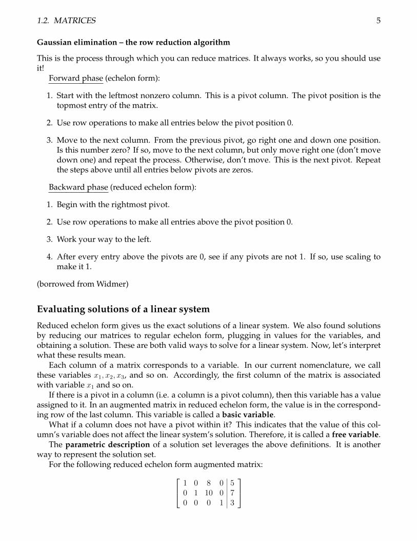
The parametric description of a solution set leverages the above definitions. It is anotherway to represent the solution set.
For the following reduced echelon form augmented matrix: 1 0 8 0 50 1 10 0 70 0 0 1 3
6 CHAPTER 1. SYSTEMS OF LINEAR EQUATIONS
its parametric description is x1 = 5
x2 = 7
x3 is freex4 = 3
Existence and uniqueness (part 2) of matrices
If the bottom row of an augmented matrix is all zero EXCEPT for the rightmost entry, then thematrix will be inconsistent.
Visually, if the bottom row of an augmented matrix looks like this:[0 . . . 0 | b
]then this system is inconsistent.
Furthermore, if a system is consistent and does not contain any free variables, it has exactlyone solution. If it contains one or more free variables, it has infinitely many solutions.
1.3 Vectors and vector equations
Back when we discussed the different kinds of solutions of a linear system, we assigned eachvariable of the system x1, x2, . . . , xn its own column. Whatever number is its subscript is whichevercolumn it represented in the matrix.
In fact, we’ll now define these individual columns to be called vectors. Specifically, we callthem column vectors: they have m number of rows but only one column. They are matrices oftheir own right.
Row vectors also exist, and have n columns but just one row. They are rarely used, andusually, the term vector refers to column vectors. (From now on, we will refer to column vectorssimply as vectors unless otherwise specified.)
We represent the set of all vectors with a certain dimension n by Rn. Note that n is the number
of rows a vector has. For instance, the vector ~v =
[43
]has two rows, so it is a vector within the
set R2.Two vectors are equal if and only if:
• they have the same dimensions
• the corresponding entries on each vector are equal
Vector operations
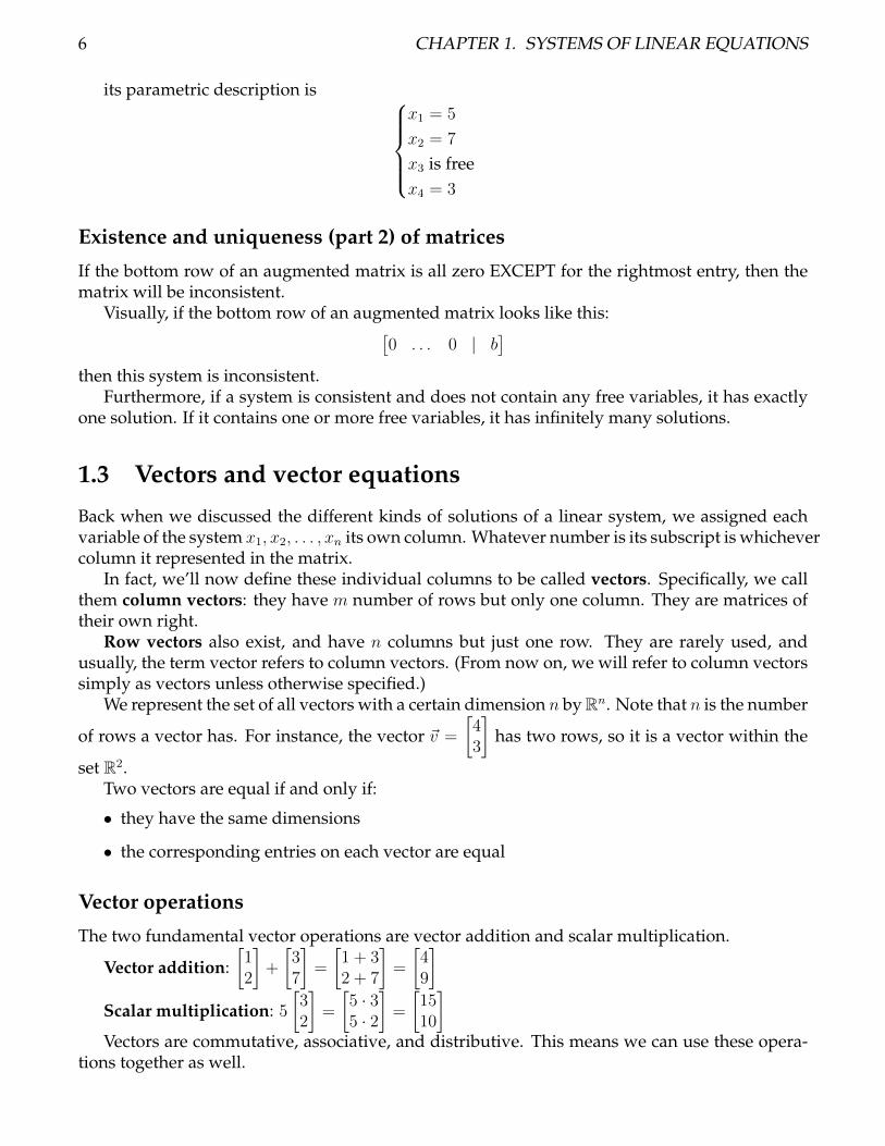
The two fundamental vector operations are vector addition and scalar multiplication.
Vector addition:[12
]+
[37
]=
[1 + 32 + 7
]=
[49
]Scalar multiplication: 5
[32
]=
[5 · 35 · 2
]=
[1510
]Vectors are commutative, associative, and distributive. This means we can use these opera-
tions together as well.
1.4. LINEAR COMBINATIONS 7
Vectors and matrices
A set of vectors can themselves form a matrix by being columns of a matrix. For instance, if
we are given ~v =
134
, ~u =
952
, ~w =
786
, and they are all within the set A, then they can be
represented as a matrix:
A =
1 9 73 5 84 2 6
Combining vectors
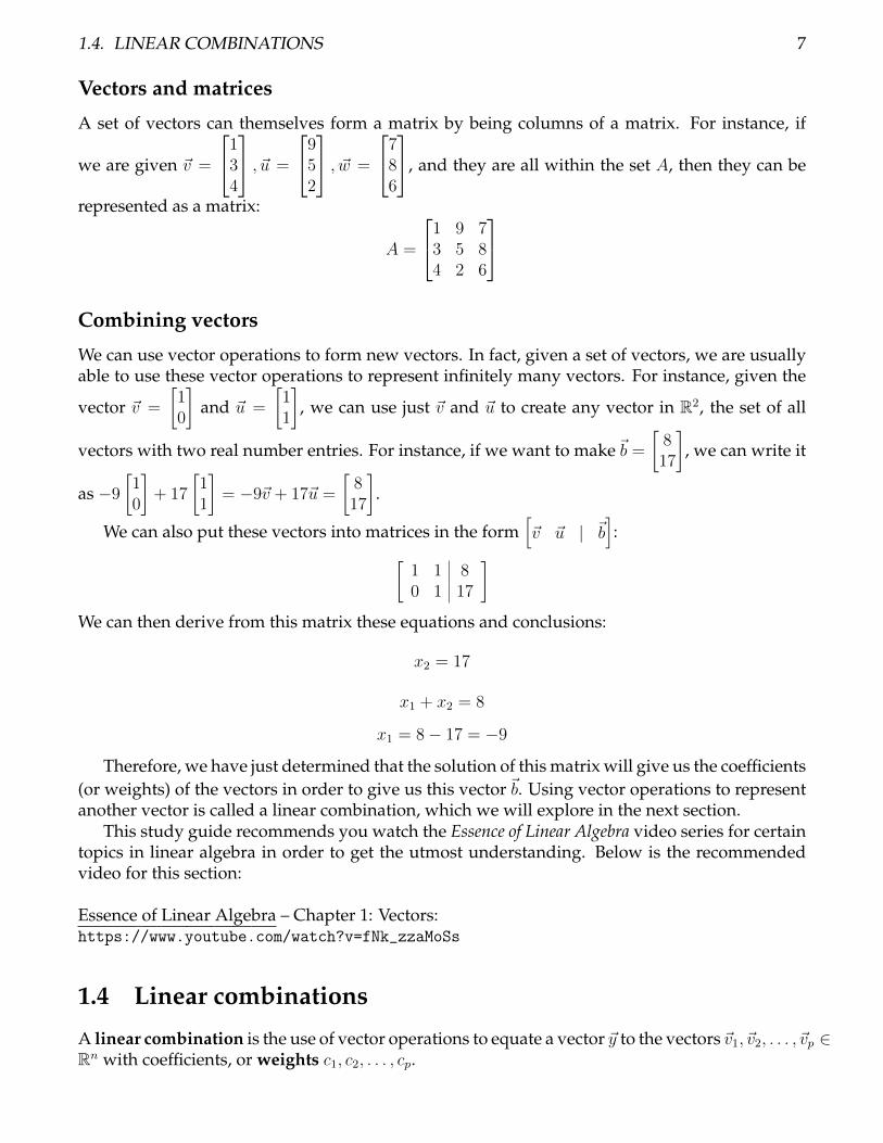
We can use vector operations to form new vectors. In fact, given a set of vectors, we are usuallyable to use these vector operations to represent infinitely many vectors. For instance, given the
vector ~v =
[10
]and ~u =
[11
], we can use just ~v and ~u to create any vector in R2, the set of all
vectors with two real number entries. For instance, if we want to make~b =[817
], we can write it
as −9[10
]+ 17
[11
]= −9~v + 17~u =
[817
].
We can also put these vectors into matrices in the form[~v ~u | ~b
]:[
1 1 80 1 17
]We can then derive from this matrix these equations and conclusions:
x2 = 17
x1 + x2 = 8
x1 = 8− 17 = −9
Therefore, we have just determined that the solution of this matrix will give us the coefficients(or weights) of the vectors in order to give us this vector~b. Using vector operations to representanother vector is called a linear combination, which we will explore in the next section.
This study guide recommends you watch the Essence of Linear Algebra video series for certaintopics in linear algebra in order to get the utmost understanding. Below is the recommendedvideo for this section:
Essence of Linear Algebra – Chapter 1: Vectors:https://www.youtube.com/watch?v=fNk_zzaMoSs
1.4 Linear combinations
A linear combination is the use of vector operations to equate a vector ~y to the vectors ~v1, ~v2, . . . , ~vp ∈Rn with coefficients, or weights c1, c2, . . . , cp.
8 CHAPTER 1. SYSTEMS OF LINEAR EQUATIONS
~y = c1~v1 + c2~v2 + · · ·+ cp~vp
An example of a linear combination is 3~v1 − 2~v2.
Span
The possible linear combinations that can result from a set of vectors {~v1, ~v2, . . . , ~vp} is called thespan.
The span is simply where this linear combination can reach. The span of ~v1 =
[12
]is simply
the line parallel to ~v1. Notice you can’t make much else out of that except scaling it. However, if
you add ~v2 =[01
]to the mix, you can now create a linear combination to get ANY value in R2 or
the 2D plane. That means these two vectors’ possibilities spans R2. For instance,[920
]= 9~v1+2~v2.
We say that a vector ~y is in the span of {~v1, ~v2, ~v3}, etc. through the notation ~y ∈ Span{~v1, ~v2, ~v3}.The formal definition of span: if ~v1, ~v2, . . . , ~vp ∈ Rn, then the set of all linear combinations
of ~v1, ~v2, . . . , ~vp is denoted by Span{~v1, ~v2, . . . , ~vp} and is called the subset of Rn spanned by~v1, ~v2, . . . , ~vp:
Span{~v1, ~v2, . . . , ~vp} = {c1~v1 + c2~v2 + · · ·+ cp~vp : c1, c2, . . . , cp are scalars.}
This study guide recommends you watch the Essence of Linear Algebra video series for certaintopics in linear algebra in order to get the utmost understanding. Below is the recommendedvideo for this section:
Essence of Linear Algebra – Chapter 2: Linear combinations, span, and basis vectors:https://www.youtube.com/watch?v=k7RM-ot2NWY
(Note that basis vectors will not be covered until Chapter 2.)
Existence and uniqueness (part 3) of linear combinations
If there is a solution to the vector equation x1~v1+x2~v2+· · ·+xp~vp = ~b, then there is a solution to itsequivalent augmented matrix:
[~v1 ~v2 . . . ~vp ~b
]. The solution to the equivalent augmented
matrix are in fact the weights of the vector equation. That means we can get x1, x2, . . . , xp fromreducing the equivalent augmented matrix.
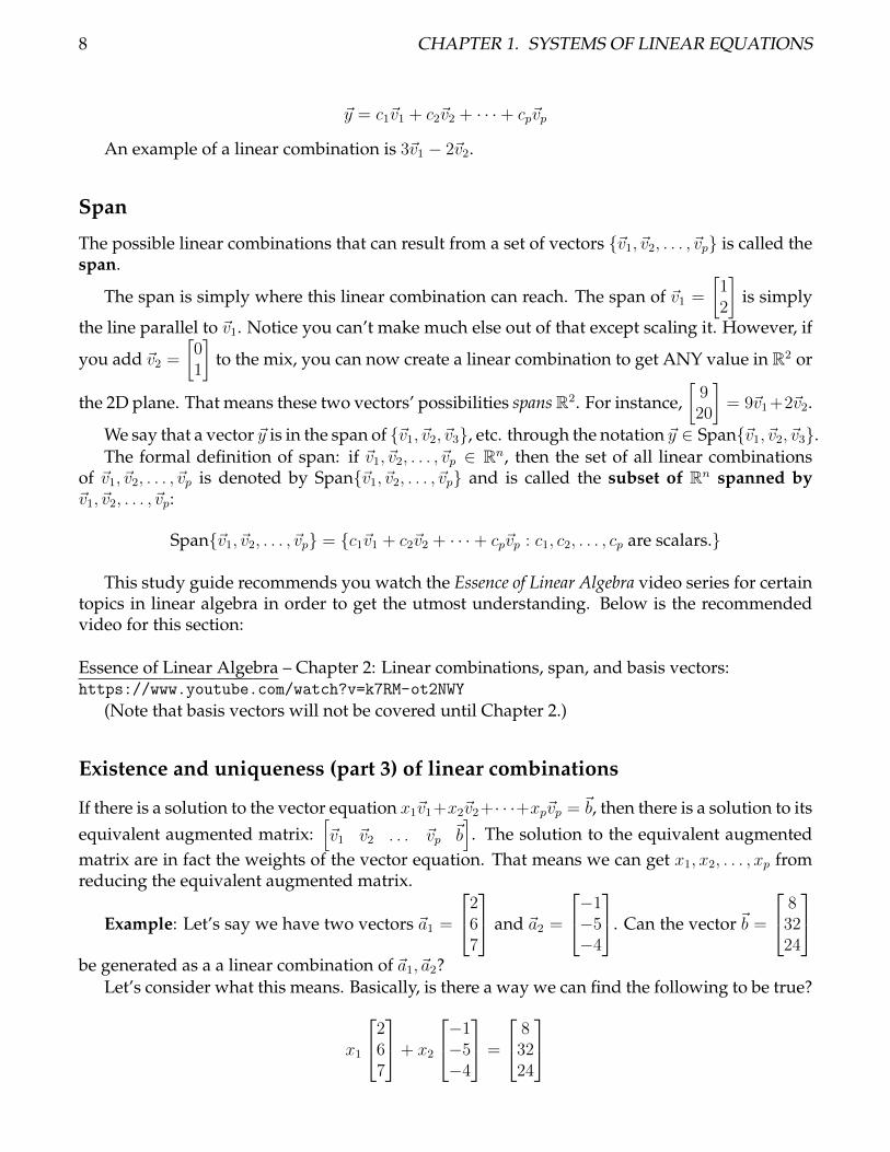
Example: Let’s say we have two vectors ~a1 =
267
and ~a2 =
−1−5−4
. Can the vector ~b =
83224
be generated as a a linear combination of ~a1,~a2?
Let’s consider what this means. Basically, is there a way we can find the following to be true?
x1
267
+ x2
−1−5−4
=
83224
1.4. LINEAR COMBINATIONS 9
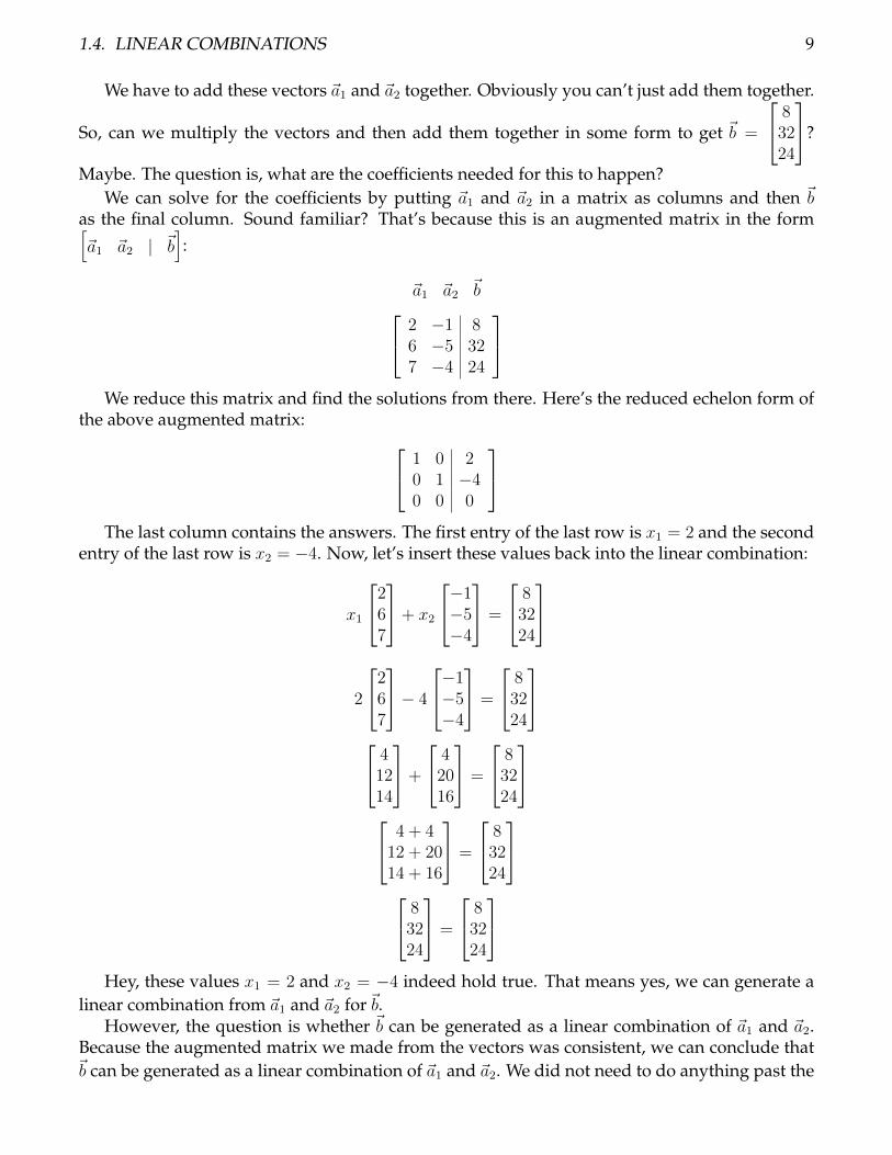
We have to add these vectors ~a1 and ~a2 together. Obviously you can’t just add them together.
So, can we multiply the vectors and then add them together in some form to get ~b =
83224
?
Maybe. The question is, what are the coefficients needed for this to happen?We can solve for the coefficients by putting ~a1 and ~a2 in a matrix as columns and then ~b
as the final column. Sound familiar? That’s because this is an augmented matrix in the form[~a1 ~a2 | ~b
]:
~a1 ~a2 ~b 2 −1 86 −5 327 −4 24
We reduce this matrix and find the solutions from there. Here’s the reduced echelon form of
the above augmented matrix: 1 0 20 1 −40 0 0
The last column contains the answers. The first entry of the last row is x1 = 2 and the second
entry of the last row is x2 = −4. Now, let’s insert these values back into the linear combination:
x1
267
+ x2
−1−5−4
=
83224
2
267
− 4
−1−5−4
=
83224
41214
+
42016
=
83224
4 + 412 + 2014 + 16
=
83224
83224
=
83224
Hey, these values x1 = 2 and x2 = −4 indeed hold true. That means yes, we can generate a
linear combination from ~a1 and ~a2 for~b.However, the question is whether ~b can be generated as a linear combination of ~a1 and ~a2.
Because the augmented matrix we made from the vectors was consistent, we can conclude that~b can be generated as a linear combination of ~a1 and ~a2. We did not need to do anything past the
10 CHAPTER 1. SYSTEMS OF LINEAR EQUATIONS
reduced echelon form. We just needed to see whether the augmented matrix was consistent.
For this same example, is~b in the span of {~a1,~a2}?The span refers to the possible combinations of a linear combination. Since ~b is a possible
linear combination of {~a1,~a2}, then yes,~b is in the span of {~a1,~a2}.
To recap, ~b generated as a linear combination of ~a1,~a2 is the same question as whether ~b is inthe span of ~a1,~a2. They are both proven by seeing whether the augmented matrix of
[~a1 ~a2 ~b
]is consistent.
1.5 Basic matrix multiplication
To prepare for our next section, we will first jump to a limited scope of matrix multiplicationwhere we are multiplying a matrix by a vector.
We can multiply matrices by each other. This operation multiplies the entries in a certainpattern. We can only multiply two matrices by each other if the first matrix’s number of columnsis equal to the second matrix’s number of rows.
To be clear, let’s say we have the first matrix and second matrix:
• The number of columns of the first matrix must equal the number of rows of the secondmatrix.
• The resulting matrix will have the number of rows that the first matrix has and the numberof columns that the second matrix has.
For instance, we can multiply: [1 2 3
] 456
but not [
1 8] 42
3
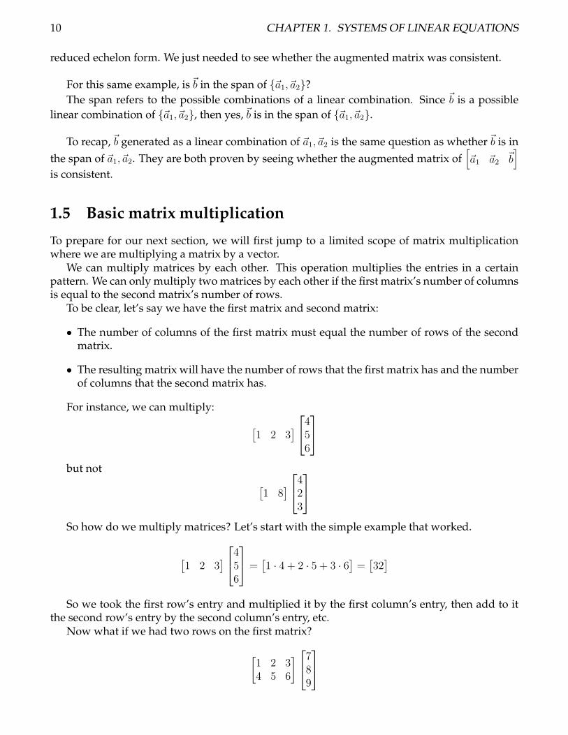
So how do we multiply matrices? Let’s start with the simple example that worked.
[1 2 3
] 456
=[1 · 4 + 2 · 5 + 3 · 6
]=[32]
So we took the first row’s entry and multiplied it by the first column’s entry, then add to itthe second row’s entry by the second column’s entry, etc.
Now what if we had two rows on the first matrix?
[1 2 34 5 6
]789
1.6. THE MATRIX EQUATION A ~X = ~B 11
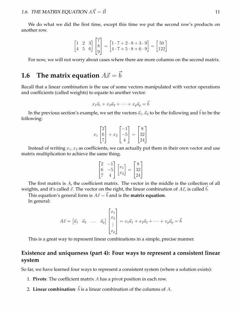
We do what we did the first time, except this time we put the second row’s products onanother row.
[1 2 34 5 6
]789
=
[1 · 7 + 2 · 8 + 3 · 94 · 7 + 5 · 8 + 6 · 9
]=
[50122
]For now, we will not worry about cases where there are more columns on the second matrix.
1.6 The matrix equation A~x = ~b
Recall that a linear combination is the use of some vectors manipulated with vector operationsand coefficients (called weights) to equate to another vector.
x1~a1 + x2~a2 + · · ·+ xp~ap = ~b
In the previous section’s example, we set the vectors ~a1,~a2 to be the following and~b to be thefollowing:
x1
267
+ x2
−1−54
=
83224
Instead of writing x1, x2 as coefficients, we can actually put them in their own vector and use
matrix multiplication to achieve the same thing.2 −16 −57 4
[x1x2
]=
83224
The first matrix is A, the coefficient matrix. The vector in the middle is the collection of all
weights, and it’s called ~x. The vector on the right, the linear combination of A~x, is called~b.This equation’s general form is A~x = ~b and is the matrix equation.In general:
A~x =[~a1 ~a2 . . . ~ap
]x1x2...xp
= x1~a1 + x2~a2 + · · ·+ xp~ap = ~b
This is a great way to represent linear combinations in a simple, precise manner.
Existence and uniqueness (part 4): Four ways to represent a consistent linearsystem
So far, we have learned four ways to represent a consistent system (where a solution exists):
1. Pivots: The coefficient matrix A has a pivot position in each row.
2. Linear combination: ~b is a linear combination of the columns of A.
12 CHAPTER 1. SYSTEMS OF LINEAR EQUATIONS
3. Span: ~b is in the span of the columns of A.
4. Matrix equation: If A~x = ~b has a solution.
1.7 Homogeneous linear systems
A homogeneous linear system is a special kind of linear system in the form A~x = ~b where~b = ~0.In other words, a homogeneous linear system is in the form A~x = ~0.What gives about them? They have some special properties.
• All homogeneous systems have at least one solution. This solution is called the trivialsolution and it’s when ~x = ~0. Of course A ·~0 = ~0 is true; that’s why we call it trivial!
• But the real question is, is there a case where a homogeneous system A~x = ~0 when ~x 6= ~0?If such a solution exists, it’s called a nontrivial solution.
• How do we know if there is a nontrivial solution? This is only possible when A~x = ~0 has afree variable. When a free variable is in the system, it allows ~x 6= 0 while A~x = 0.
• Therefore, we can say whenever a nontrivial solution exists for a homogeneous system,it has infinitely many solutions. When only the trivial solution exists in a homogeneoussystem, the system has a unique solution (uniqueness).
Parametric vector form
When we have free variables, we describe basic variables with relation to the free variables. Wegroup the weights of the free variables to the basic variables through parametric vector form.
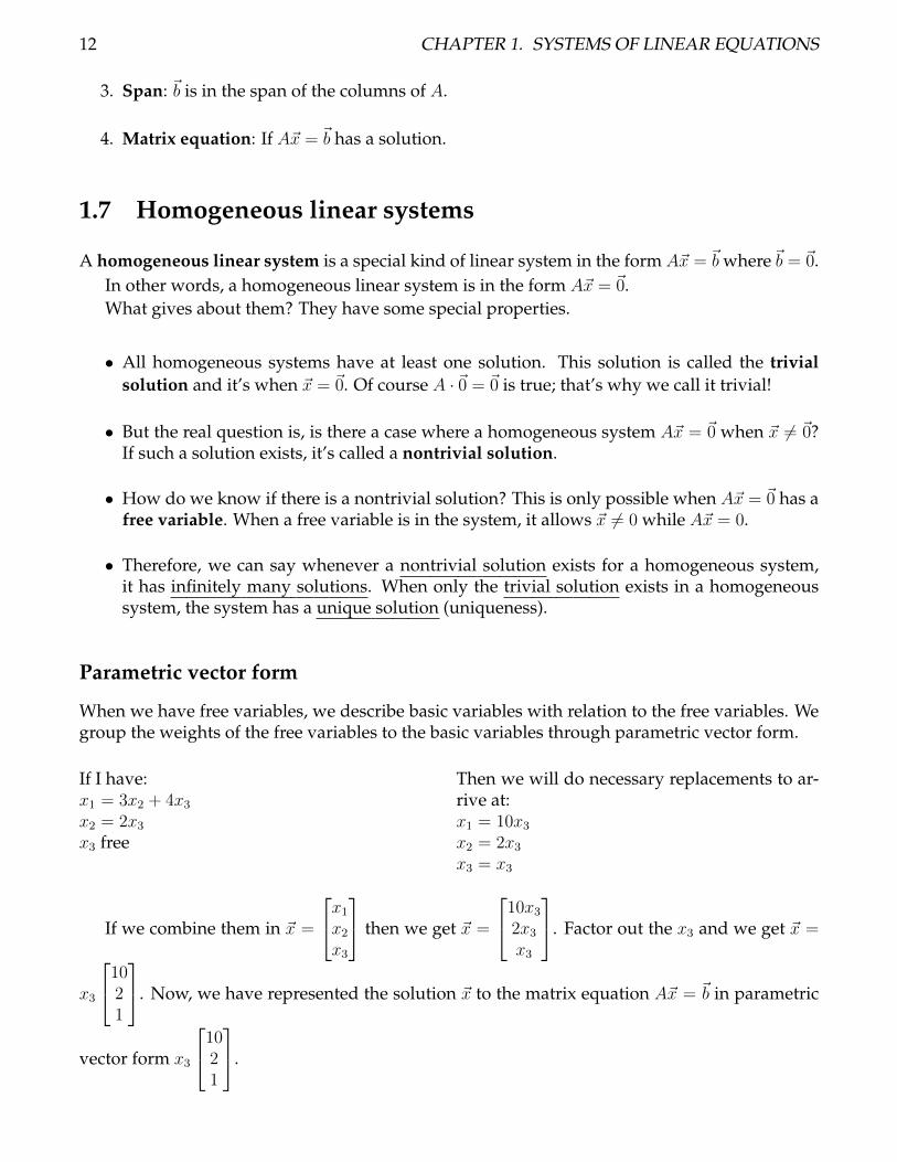
If I have:x1 = 3x2 + 4x3x2 = 2x3x3 free
Then we will do necessary replacements to ar-rive at:x1 = 10x3x2 = 2x3x3 = x3
If we combine them in ~x =
x1x2x3
then we get ~x =
10x32x3x3
. Factor out the x3 and we get ~x =
x3
1021
. Now, we have represented the solution ~x to the matrix equation A~x = ~b in parametric
vector form x3
1021
.
1.8. LINEAR INDEPENDENCE 13
Non-homogeneous linear systems in terms of homogeneous linear systems
What linear system is a non-homogeneous linear system? Basically, it’s anything where A~x 6= ~0.So, basically most matrix equations.
What’s fascinating is that non-homogeneous linear systems with infinitely many solutionscan actually be represented through homogeneous linear systems that have nontrivial solutions.This is because non-homogeneous linear systems are in fact homogeneous linear systems with atranslation by a certain constant vector ~p, where ~x = ~p + t~v. t~v is where all of the free variablesare located.
And guess what? Since this system has infinitely many solutions, the translation is taken outwhen A~x = ~0. That means, for a system with infinitely many solutions (i.e. one that can bewritten in parametric vector form), the nonconstant vector ~v (the one with the free variables),without the constant vector ~p, is a possible solution!
1.8 Linear independence
Now, within our linear combination, could we have duplicate vectors? Yes. Graphically speak-ing, if two vectors are multiples of each other, they would be parallel. The whole point of linearcombinations is to make new vectors. What use is two vectors that are multiples of each other?That’s redundant.
This is where the concept of linear independence comes in. Are there any redundant vari-ables in the linear combination? Or, are there any redundant rows in a reduced matrix? If so,there are redundancies and therefore we say the combination is linearly dependent. If nothingis redundant, then it’s linearly independent.
Mathematically, however, we have a formal way of defining linear independence. If the linearcombination x1~v1 + x2~v2 + . . . xp~vp = ~0 has only the trivial solution, then it’s linearly independent.Otherwise, if there exists a nontrivial solution, it must be linearly dependent.
Why is that? If there are redundant vectors, then there exists weights for them to cancel each
other out. Let’s say we have two vectors ~v1 =
123
, ~v2 =
246
. Clearly, ~v2 is a multiple of ~v1.
So we can say 2~v1 = ~v2. We can rearrange this to get 2~v1 − 1~v2 = ~0. Therefore, per our formaldefinition, {~v1, ~v2} is linearly dependent.
If a set of vectors are linearly dependent, then there are infinitely many ways to make acombination. Therefore, there would be infinitely many solutions for A~x = ~b. However, if aset of vectors are linearly independent, then there would only be at most one way to form thesolution for A~x = ~b.
This leads us to a conceptual connection that is very important: if a set of vectors are lin-early independent, at most one solution can be formed. This means linear independence impliesuniqueness of solution.
Linear independence of a set of one vector
A set with one vector contained within is linearly independent unless this vector is the zerovector. The zero vector is linearly dependent but has only the trivial solution.
14 CHAPTER 1. SYSTEMS OF LINEAR EQUATIONS123
is linearly independent.[00
]is linearly dependent and has only the trivial solution.
Linear independence of a set of two vectors
Given two vectors ~v, ~u, then this set is linearly independent as long as ~v is not in the span of ~u. Itcould also be the other way around, but the same result still holds true.
Linear independence of a set of multiple vectors
We have several rules for determining linear dependence of a set of multiple vectors. If one ruleholds true, then the set is linearly dependent.
• If at least one of the vectors in the set is a linear combination of some other vectors in theset, then the set is linearly dependent. (Note that not all have to be a linear combination ofeach other for this to hold true. Just one needs to be a linear combination of others.)
• If there are more columns than rows in a coefficient matrix, that system is linearly depen-dent. Why? Recall that the number of entries a vector has is equivalent to the number ofdimensions it contains. If there are more vectors than dimensions, the vectors will be re-
dundant within these dimensions. For instance, ~v1 =[12
]only spans a line in R2. If we add
~v2 =
[01
]to the set, we can now span all of R2 because ~v1 is not parallel to ~v2. But if we add
~v3 =
[−10
], it doesn’t add anything new to the span. We’re still in R2 but with a redundant
vector. Furthermore, ~v1 = 2~v2 − 1~v3, so clearly that would be a linearly dependent set ofvectors.
• If a set contains the zero vector ~0, then the set is linearly dependent. It’s easy to create thezero vector with any vector; just make the weight 0, lol.
1.9 Linear transformations
We have studied the matrix equation A~x = ~b. This equation is kind of like y = mx + b, whichis just a relation. These relations can be represented as functions in regular algebra as f(x) =mx + b. Now, we will transition to the equivalent of functions in linear algebra, called lineartransformations.
A linear transformation, also called a function or mapping, is where we take the vector ~xand manipulate it to get the result T (~x). This is the same concept as turning x into f(x). Howdo we manipulate it? We have several options, but for now, we will stick with the coefficientmatrix A. Using the coefficient matrix for manipulation means we are using a special form oflinear transformation called a matrix transformation. (Note of clarification: If we talk about A,then we are referring to a matrix transformation. Otherwise, we are referring to a general lineartransformation.)

1.9. LINEAR TRANSFORMATIONS 15
For the coefficient matrix A with size m × n (where m is the number of rows and n is thenumber of columns), the number of columns n it has is the domain (Rn) while the number ofrows m it has is the codomain (Rm). The codomain is different from the range.
Specifically, the transformed vector ~x itself, T (~x), is called the image of ~x under T . Note thatthe image is like the~b in A~x = ~b, and in fact, T (~x) = ~b.
Something to keep in mind: matrix equations can have no solutions, one solution, or in-finitely many solutions. If no ~x can form an image, it means there’s no solutions. If only one ~xforms an image, then there is only one solution. But if we can find more than one ~x (i.e. there’sprobably a basic variable) then we have infinitely many solutions and not a unique solution.
Why isn’t the codomain the range? Well, the range is the places where the solution to thismatrix exists. The image is the actual vector ~x transformed, while the codomain is just the newdomain where the image resides after this transformation has shifted. Not all of the codomainis in the range of the transformation. Remember, this is linear algebra, and we’re shifting the di-mensions here with these transformations, so we have to differentiate between which dimensionwe’re in before and after. If A~x = ~b, then~b is in the range of the transformation ~x 7→ A~x.
By the way, the notation to represent a transformation’s domain to codomain is:
T : Rn 7→ Rm
Note that 7→ is read as ”maps to”, so that’s why we’ll call use the terms transformations andmappings interchangeably. It’s just natural!
Properties of linear transformations
It’s important to note that matrix transformations are a specific kind of linear transformation, soyou can apply these properties to matrix transformations, but they don’t solely apply to matrixtransformations. Also, don’t forget later on that these properties hold true for other kinds oflinear transformations. With that in mind, the following properties apply to all linear transfor-mations:
• T (~u+ ~v) = T (~u) + T (~v), for ~u,~v ∈ Domain{T}
• T (c~u) = cT (~u), for c ∈ R, ~u ∈ Domain{T}
• T (~0) = ~0 - oh yeah, that’s right. Those ”linear functions” y = mx+ b with b 6= 0 you learnedabout in Algebra I? They’re not actually ”linear functions” in linear algebra.
So why do these properties even matter? In problems, you are given T (~u) but not ~u itself (i.e.~b and not ~x inA~x = ~b), so you must isolate T (~u) from these operations to do anything meaningfulwith it.
This study guide recommends you watch the Essence of Linear Algebra video series for certaintopics in linear algebra in order to get the utmost understanding. Below is the recommendedvideo for this section:
Essence of Linear Algebra – Chapter 3: Linear transformations and matrices:https://www.youtube.com/watch?v=kYB8IZa5AuE
16 CHAPTER 1. SYSTEMS OF LINEAR EQUATIONS
1.10 The matrix of a linear transformation
In the previous section, we mainly dealt with ~x in the matrix equation A~x = ~b. Why is A~x = ~b atransformation? Because, every linear transformation that satisfies Rm 7→ Rn is a matrix trans-formation. (Note: This means only linear transformations with Rm 7→ Rn is a matrix transfor-mation. What was said before about not all linear transformations being matrix transformationsstill holds true.) And because they are matrix transformations, we can use the form ~x 7→ A~x torepresent our transformations. In this section, we will shift the focus from ~x to A.
Now, when we map ~x 7→ A~x, we have technically do have a coefficient in the front of the lone~x. So really, we should say I~x 7→ A~x. What matrix I always satisfies ~x = I~x? The identity matrixIn, which is a matrix size n× n with all zeroes except for ones down the diagonal.
I2 =
[1 00 1
], I3 =
1 0 00 1 00 0 1
, I4 =1 0 0 00 1 0 00 0 1 00 0 0 1
, etc.
Why does this matter? Well, in I~x 7→ A~x, ~x is on both sides. So really, the transformationrepresents a change from I , the identity matrix, to A. We shall name A the standard matrix.
The columns of the identity matrix, which we shall call {~e1, ~e2, . . . , ~en}, correlate to the columnsof the standard matrix, which are just transformations of the identity matrix’s columns (i.e.A = [T (~e1)T (~e2) . . . T (~en)]).
This study guide recommends you watch the Essence of Linear Algebra video series for certaintopics in linear algebra in order to get the utmost understanding. Below is the recommendedvideo for this section:
Essence of Linear Algebra – Footnote, Nonsquare matrices as transformations between dimen-sions:https://www.youtube.com/watch?v=v8VSDg_WQlA
Geometric transformations in R2
As an aside, some of these standard matrices perform geometric transformations in one of theseclasses:
• Reflections
• Contractions and expansions
• Shears - keeping one component constant while multiplying another component by ascalar
• Projections - ”shadows” onto a lower dimension (in this case, R1)
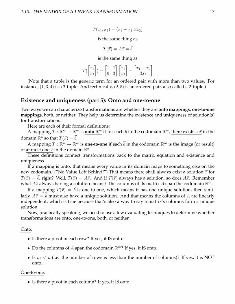
Another vector representation format
We can write vectors another way: ~x =
[x1x2
]= (x1, x2). This comes in handy when we want to
write a transformation as a tuple, like we do for a function: T (x1, x2) = (x1+x2, 3x2) =
[x1 + x23x2
].
1.10. THE MATRIX OF A LINEAR TRANSFORMATION 17
T (x1, x2) = (x1 + x2, 3x2)
is the same thing as
T (~x) = A~x = ~b
is the same thing as
T (
[x1x2
]) =
[1 10 3
] [x1x2
]=
[x1 + x23x2
](Note that a tuple is the generic term for an ordered pair with more than two values. For
instance, (1, 3, 4) is a 3-tuple. And technically, (2, 5) is an ordered pair, also called a 2-tuple.)
Existence and uniqueness (part 5): Onto and one-to-one
Two ways we can characterize transformations are whether they are onto mappings, one-to-onemappings, both, or neither. They help us determine the existence and uniqueness of solution(s)for transformations.
Here are each of their formal definitions:A mapping T : Rn 7→ Rm is onto Rm if for each ~b in the codomain Rm, there exists a ~x in the
domain Rn so that T (~x) = ~b.A mapping T : Rn 7→ Rm is one-to-one if each ~b in the codomain Rm is the image (or result)
of at most one ~x in the domain Rn.These definitions connect transformations back to the matrix equation and existence and
uniqueness.If a mapping is onto, that means every value in its domain maps to something else on the
new codomain. (”No Value Left Behind!”) That means there shall always exist a solution ~x forT (~x) = ~b, right? Well, T (~x) = A~x. And if T (~x) always has a solution, so does A~x. Rememberwhat A~x always having a solution means? The columns of its matrix A span the codomain Rm.
If a mapping T (~x) = ~b is one-to-one, which means it has one unique solution, then simi-larly, A~x = ~b must also have a unique solution. And that means the columns of A are linearlyindependent, which is true because that’s also a way to say a matrix’s columns form a uniquesolution.
Now, practically speaking, we need to use a few evaluating techniques to determine whethertransformations are onto, one-to-one, both, or neither.
Onto:
• Is there a pivot in each row? If yes, it IS onto.
• Do the columns of A span the codomain Rm? If yes, it IS onto.
• Is m < n (i.e. the number of rows is less than the number of columns)? If yes, it is NOTonto.
One-to-one:
• Is there a pivot in each column? If yes, it IS onto.
18 CHAPTER 1. SYSTEMS OF LINEAR EQUATIONS
• Are the columns of A linearly independent? If yes, it IS one-to-one.
• Is m > n (i.e. the number of rows is greater than the number of columns)? If yes, it is NOTone-to-one.
• Are there any free variables? If yes, it is NOT one-to-one.
In summary:
• Onto mapping (also called surjective): does a solution exist? If yes, then the transforma-tion is onto. More precisely, T maps the domain Rm onto the codomain Rn.
• One-to-one mapping (also called injective): are there infinitely many solutions? (i.e. arethere any free variables in the equation?) If yes, then the transformation is NOT one-to-one.
If a transformation is one-to-one, then the columns of A will be linearly independent.If there is a pivot in every row of a standard matrix A, then T is onto.If there is a pivot in every column of a standard matrix A, then T is one-to-one.
1.11 Summary of Chapter 1: Ways to represent existence anduniqueness
The following concepts are related to or show existence of a solution:
• If a pivot exists in every row of a matrix.
• If a system is consistent.
• If weights exist for a linear combination formed from the columns of the coefficient matrixto equate the solution.
• If the solution is in the span of a set of vectors, usually the set of vectors in a linear combi-nation or the columns of the coefficient matrix.
• If there exists a solution for A~x = ~b.
• If a transformation is onto or surjective.
The following concepts are related to or show uniqueness of a solution:
• If a pivot exists in every column of a matrix.
• If there are no free variables (solely basic variables) in a solution.
• If a homogeneous linear systemA~x = ~0 has only the trivial solution where ~x = 0 is the onlysolution to A~x = ~0.
• If a solution can be expressed in parametric vector form.
• If a set of vectors is linearly independent.
• If a transformation is one-to-one or injective.
Chapter 2
Matrix algebra
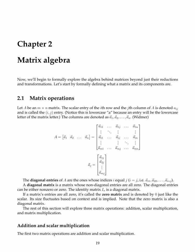
Now, we’ll begin to formally explore the algebra behind matrices beyond just their reductionsand transformations. Let’s start by formally defining what a matrix and its components are.
2.1 Matrix operations
Let A be an m× n matrix. The scalar entry of the ith row and the jth column of A is denoted aijand is called the (i, j) entry. (Notice this is lowercase ”a” because an entry will be the lowercaseletter of the matrix letter.) The columns are denoted as ~a1,~a2, . . . ,~an. (Widmer)
A =[~a1 ~a2 . . . ~an
]=
~a11 . . . ~a1j . . . ~a1n
... . . . ......
~ai1 . . . ~aij . . . ~ain...
... . . . ...~am1 . . . ~amj . . . ~amn
~aj =
~a1j~a2j
...~amj
The diagonal entries of A are the ones whose indices i equal j (i = j, i.e. ~a11,~a22, . . . ,~ai=j).A diagonal matrix is a matrix whose non-diagonal entries are all zero. The diagonal entries
can be either nonzero or zero. The identity matrix In is a diagonal matrix.If a matrix’s entries are all zero, it’s called the zero matrix and is denoted by 0 just like the
scalar. Its size fluctuates based on context and is implied. Note that the zero matrix is also adiagonal matrix.
The rest of this section will explore three matrix operations: addition, scalar multiplication,and matrix multiplication.
Addition and scalar multiplication
The first two matrix operations are addition and scalar multiplication.
19
20 CHAPTER 2. MATRIX ALGEBRA
Addition of two matrices is only possible if they share the same size. (If they are not thesame size, the operation is undefined.) Simply add up their corresponding entries to form anew, same-sized matrix. [
1 2 34 5 6
]+
[3 4 51 2 6
]=
[4 6 85 7 12
]Scalar multiplication is simply multiplying all of the entries of a matrix by a scalar value.
3
[2 4 33 2 1
]=
[6 12 99 6 3
]Now that we’ve established these simple concepts, let’s start talking about their algebraic
properties. Central to our understanding of these operations are:
1. what criteria makes matrices equal to each other (equivalence)
2. what algebraic properties these matrix operations have (commutative, associative, and dis-tributive)
So first, let’s talk about equivalence. Two matrices are equivalent if they 1. share the same sizeand 2. each of their corresponding entries are equal to each other. That’s easy.
Matrix addition and scalar multiplication have commutative, associative, and distributiveproperties.
For example, let A,B,C be matrices of the same size, and let x, y be scalars.
• Associative:(A+B) +C = A+ (B +C) - order in which you perform matrix addition does not matter.x(yA) = (xy)A - same for multiplication
• Commutative:A + B = B + A - the order of the operands (A and B) around the operator (+) does notmatterxA = Ax - same thing
• Distributive:x(A+B) = xA+ xB(x+ y)A = xA+ yA
Matrix multiplication
The last matrix operation we will learn about is matrix multiplication. Instead of multiplying ascalar by a matrix, we multiply two matrices by each other.
Why is this significant? When we make multiple linear transformations in a row, like:
~x 7→ B~x 7→ A(B~x)
then this is really equivalent to~x 7→ AB~x
2.1. MATRIX OPERATIONS 21
This study guide recommends you watch the Essence of Linear Algebra video series for certaintopics in linear algebra in order to get the utmost understanding. Below is the recommendedvideo for this section:
Essence of Linear Algebra – Chapter 4: Matrix multiplication as composition:https://www.youtube.com/watch?v=XkY2DOUCWMU
Matrix multiplication procedure expansion
We already learned some basics of matrix multiplication in section 1.5. Now, we will expand itfrom multiplying a matrix by a vector to a matrix by another matrix!
The result of a matrix multiplied by a column vector is actually always going to be a columnvector. Why? Because the number of columns a product matrix has (the result of the multipli-cation) is actually always going to be the number of columns the second matrix has. A columnvector is a matrix with one column. Therefore, the result was always a column matrix.
However, now we simply modify the multiplication procedure by doing the same thing asbefore, only now we also multiply all of the first matrix by the second column of the secondmatrix and put the values in a new column instead of adding them onto the first column’s values.
Matrix multiplication: requirements and properties
Now, in order for matrix multiplication to occur, first the number of columns the first matrix hasmust equal the number of rows the second matrix has. The resulting product matrix will havethe number of rows the first has and the number of columns that the second matrix has.
Let’s say we multiply a 3 × 5 matrix A by a 5 × 7 one B. 5 = 5, so we can move on. Theproduct matrix, AB, will have a size of 3× 7.
But what if we multiplied it in the reverse order, BA? 5 × 7 multiplied by 3 × 5? Well, 7 6= 3and therefore we actually cannot multiply in the order BA.
This is very important. The order in which matrices are multiplied do matter. Therefore,matrix multiplication is not communitative. Generally speaking, AB 6= BA.
Here are the properties of matrix multiplication:
• Associative:(AB)C = A(BC) - order in which you perform matrix multiplication does not matter.
• Distributive:(A+B)C = AC +BCA(B + C) = AB + ACx(AB) = (xA)B = A(xB)
• Identity: ImA = A = AIn
• Commutative: Lol jk it’s not commutative remember? In general, AB 6= BA.
Some things to watch out for because of the special properties of matrix multiplication!
1. In general, AB 6= BA.
2. Cancelation laws do not apply to matrix multiplication. If AB = AC, this does not meanB = C is necessarily true. It might be, rarely, but that’s not the rule in general.
22 CHAPTER 2. MATRIX ALGEBRA
3. If AB = 0, that does not mean A is 0 nor is B 0. They could both be nonzero.
One final thing. You can multiply matrices to the power of themselves (matrix exponentia-
tion) if they have the same number of rows and columns. In that case, Ak =k∏1
A (meaning A
multiplied k times), where k ∈ Z+.
2.2 Transpose and inverse matrices
Transpose
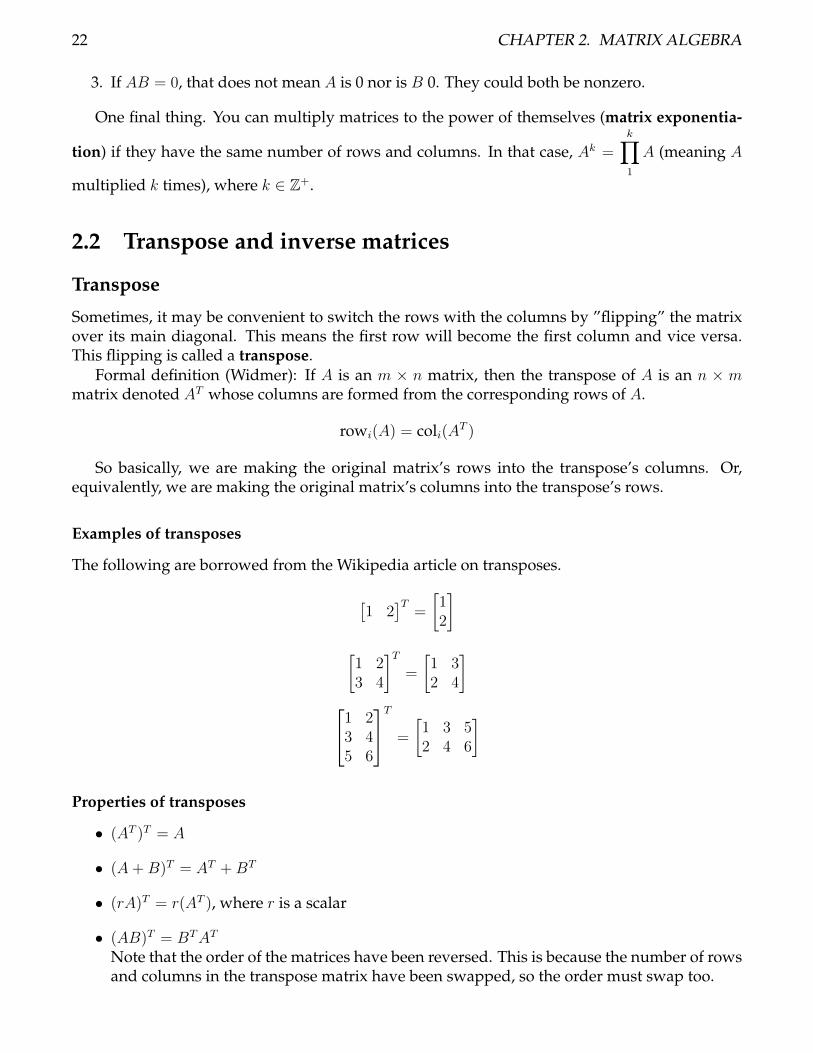
Sometimes, it may be convenient to switch the rows with the columns by ”flipping” the matrixover its main diagonal. This means the first row will become the first column and vice versa.This flipping is called a transpose.
Formal definition (Widmer): If A is an m × n matrix, then the transpose of A is an n × mmatrix denoted AT whose columns are formed from the corresponding rows of A.
rowi(A) = coli(AT )
So basically, we are making the original matrix’s rows into the transpose’s columns. Or,equivalently, we are making the original matrix’s columns into the transpose’s rows.
Examples of transposes
The following are borrowed from the Wikipedia article on transposes.
[1 2
]T=
[12
][1 23 4
]T=
[1 32 4
]1 23 45 6
T
=
[1 3 52 4 6
]
Properties of transposes
• (AT )T = A
• (A+B)T = AT +BT
• (rA)T = r(AT ), where r is a scalar
• (AB)T = BTAT
Note that the order of the matrices have been reversed. This is because the number of rowsand columns in the transpose matrix have been swapped, so the order must swap too.
2.2. TRANSPOSE AND INVERSE MATRICES 23
Inverse matrices
Let’s say we have a square matrix A, size n × n. When we multiply A by another matrix, itbecomes the identity matrix In. What is this other matrix? It’s the inverse matrix. If a matrix Aand another B produce the following results:
AB = BA = In
then they are inverses of each other/they are invertible. The inverse of matrix A is denotedA−1.
Inverses are not always possible. For one, if a matrix is not square, then it cannot have aninverse. But in certain scenarios, a square matrix may not have an inverse. These matrices arecalled singular or degenerate and will be further discussed later.
Also, both AB and BA must be true for A to be the inverse matrix of B and vice versa.Since matrix multiplication is not commutative, there are instances where AB might producethe identity matrix but not BA. In those instances, A and B are not considered inverses of eachother.
Determining the inverse of a 2× 2 matrix
There exists a computational formula to find the inverse of a 2×2 matrix. While it does not applyto any other sizes, we will later find that computing larger inverses can be done by breakingmatrices up into multiple 2× 2 matrices, and then using this formula.
A−1 =1
ad− bc
[d −b−c a
]=
1
detA
[d −b−c a
]In the matrix, a and d have swapped positions while b and c have swapped signs. Also,
the denominator is called something special that will be of great significance in the comingchapters—it’s called the determinant, and for a 2 × 2 matrix, it is calculated by ad − bc. No-tice that when detA = ad − bc = 0, the denominator would be zero and that would make theinverse impossible to calculate. This means that a matrix has no inverse (i.e. it is singular) if andonly if its determinant is equal to zero (i.e. detA = 0).
A matrix A is only invertible when detA = ad− bc 6= 0.
Inverses and matrix equations
In the last chapter, we solved the matrix equation A~x = ~b through various methods mainlyboiling down to Gaussian row reduction. But now, we can introduce another, more intuitiveway to solve for it. Why can’t we ”cancel out” the A on the left side and move it to the right side,in a way?
With inverses, we can! If A is an invertible n× n matrix, then A~x = ~b has the unique solution~x = A−1~b. Note the order of the latter part. It is A−1~b, not~bA−1. (It has been struck out because itis wrong and we don’t want you getting the wrong idea here.)
We can write A~x = ~b as ~x = A−1~b if A is invertible.
This is kind of like division in scalar algebra (regular algebra you did in high school). Re-member though, that division is not a defined operation in matrix algebra, so this is one of the”analogs” we can come up with.
24 CHAPTER 2. MATRIX ALGEBRA
Properties of invertible matrices
• If A is an invertible matrix, then A−1 is invertible and (A−1)−1 = A.
• If A and B are invertible n× n matrices, then AB is invertible and (AB)−1 = B−1A−1.
• If A is an invertible matrix, AT is invertible and (AT )−1 = (A−1)T .This property is derived from an inverse’s inherent commutative property.
Inverse matrices and row equivalence
This subsection will explore the connection between matrix multiplication and row equivalence.Up to this point, we have identified that invertible matrices have the following property:
AA−1 = A−1A = I is always true. That is, an invertible matrix multiplied by its inverse matrix isalways equal to the identity matrix, regardless of the order. This means we can find the inversematrix using matrix multiplication.
However, we can also use the three elementary row operations (replacement, swap, andscale) to substitute for a series of matrix multiplications like A−1A = I (which are really transfor-mations). If we can use these row operations to get from A to I , that means A is row equivalentto the identity matrix. We learned about row equivalence back in the first half of Chapter 1.
A square matrix A is row equivalent to the identity matrix if and only if A is invertible. Thesetwo things mean the same thing!
Using this profound connection, we can also start considering each elementary row operationas a matrix that is multiplied onto the matrix A. We call these matrices elementary matrices.
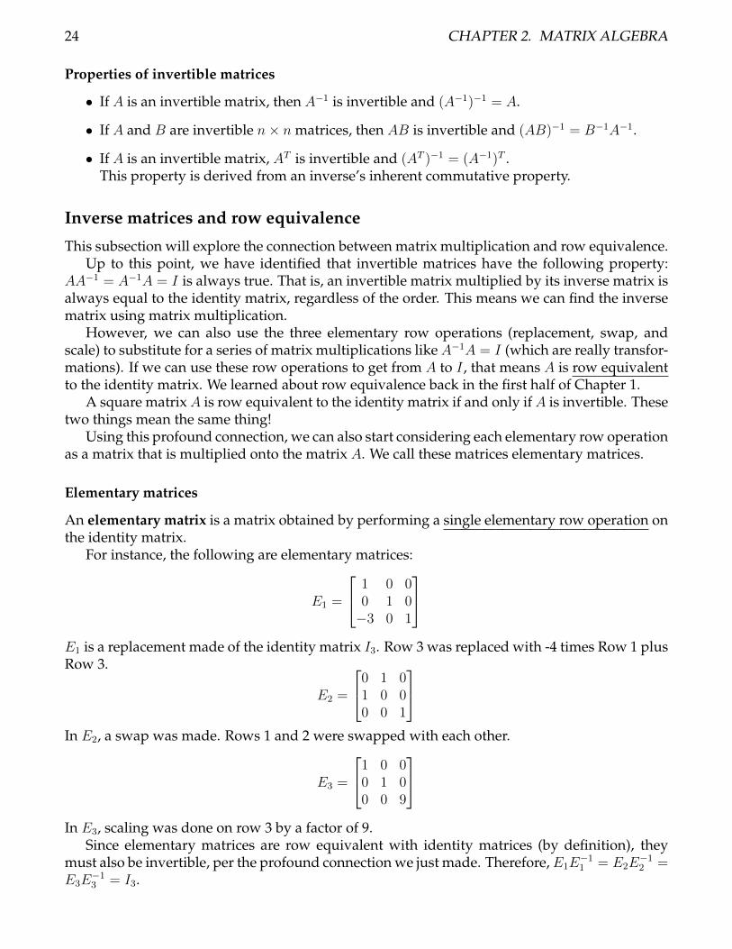
Elementary matrices
An elementary matrix is a matrix obtained by performing a single elementary row operation onthe identity matrix.
For instance, the following are elementary matrices:
E1 =
1 0 00 1 0−3 0 1
E1 is a replacement made of the identity matrix I3. Row 3 was replaced with -4 times Row 1 plusRow 3.
E2 =
0 1 01 0 00 0 1
In E2, a swap was made. Rows 1 and 2 were swapped with each other.
E3 =
1 0 00 1 00 0 9
In E3, scaling was done on row 3 by a factor of 9.
Since elementary matrices are row equivalent with identity matrices (by definition), theymust also be invertible, per the profound connection we just made. Therefore,E1E
−11 = E2E
−12 =
E3E−13 = I3.
2.3. CHARACTERISTICS OF INVERTIBLE MATRICES: THE INVERTIBLE MATRIX THEOREM25
Why are elementary matrices important? Because the matrix multiplication E1A is the sameas the row operation ”A : R3 → R3+(−4)R1”. This is how we represent row operations throughmatrix operations.
Row equivalence of elementary matrices
Interestingly enough, the same sequence of row operations/multiplication made on A to get toI will get I to A−1. More precisely, this means A→ I is row equivalent to I → A−1.
This means if you have an augmented matrix [A|I] and you perform a sequence of elementaryrow operations on it to getA on the left turned into I , you will simultaneously turn I on the rightto A−1, which is A’s inverse.
[A|I]→ [I|A−1]
Then, if we consider this sequence of elementary row operations as a sequence of matricesmultiplying by each other, we can use elementary matrices to represent a sequence of row op-erations as: Ep . . . E2E1. Notice that the last row operation Ep is on the left and the first rowoperation E1 is on the right. That is because order matters in matrix multiplication and theinvertible matrix A will be to the right of E1.
We can conclude that a sequence of elementary matricesEp . . . E2E1 that allowsEp . . . E2E1A =I to be true will also make Ep . . . E2E1I = A−1. Therefore:
Ep . . . E2E1 = A−1
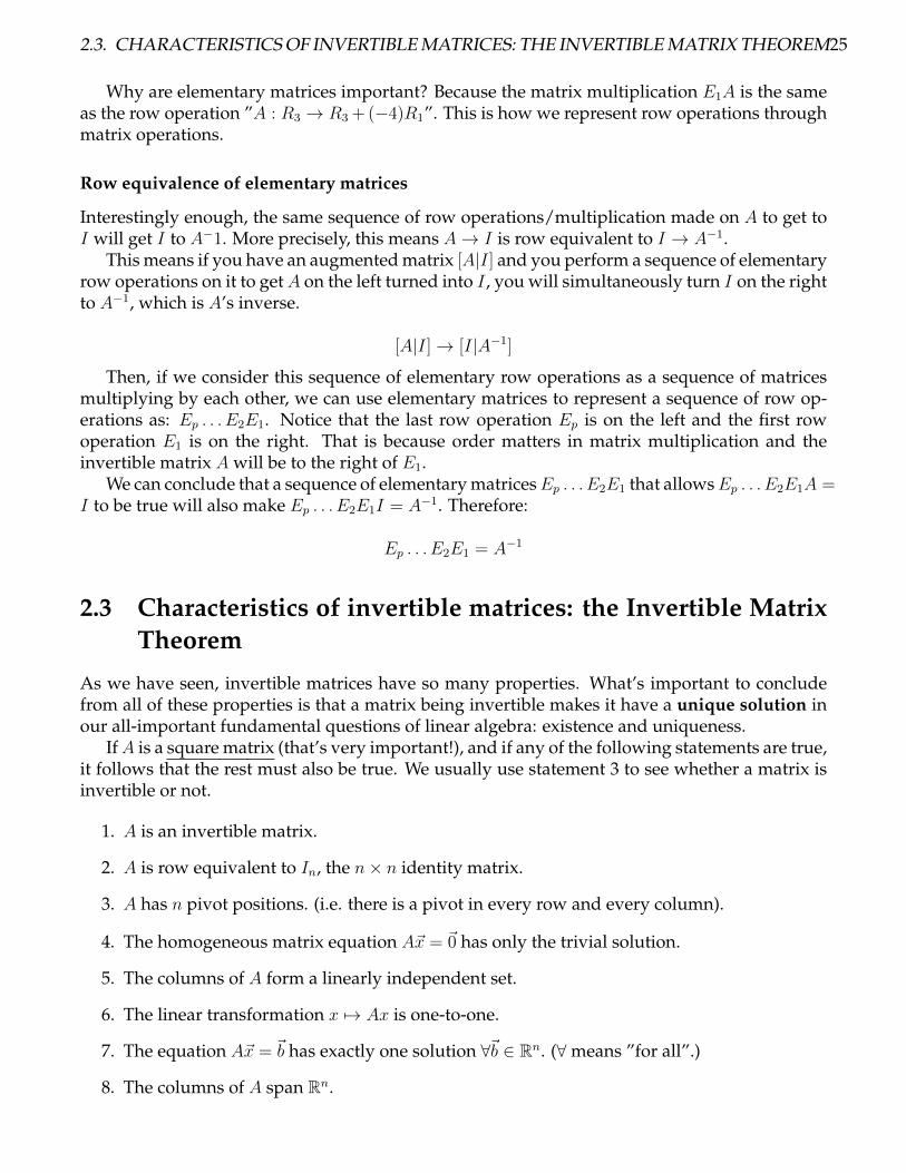
2.3 Characteristics of invertible matrices: the Invertible MatrixTheorem
As we have seen, invertible matrices have so many properties. What’s important to concludefrom all of these properties is that a matrix being invertible makes it have a unique solution inour all-important fundamental questions of linear algebra: existence and uniqueness.
IfA is a square matrix (that’s very important!), and if any of the following statements are true,it follows that the rest must also be true. We usually use statement 3 to see whether a matrix isinvertible or not.
1. A is an invertible matrix.
2. A is row equivalent to In, the n× n identity matrix.
3. A has n pivot positions. (i.e. there is a pivot in every row and every column).
4. The homogeneous matrix equation A~x = ~0 has only the trivial solution.
5. The columns of A form a linearly independent set.
6. The linear transformation x 7→ Ax is one-to-one.
7. The equation A~x = ~b has exactly one solution ∀~b ∈ Rn. (∀means ”for all”.)
8. The columns of A span Rn.
26 CHAPTER 2. MATRIX ALGEBRA
9. The linear transformation x 7→ Ax maps Rn onto Rn.
10. There is an n× n matrix C so that CA = In.
11. There is an n× n matrix D so that AD = In. C = D always.
12. AT is an invertible matrix.
To reiterate, this theorem only applies to square matrices! Regular non-square rectangularmatrices do NOT obey this theorem.
(This theorem will be expanded with new statements in later sections.)
Invertible linear transformations
In algebra, we can say that a function g(x) is the inverse of f(x) if g(f(x)) = (g ◦ f)(x) = x. Wecan say the same thing for transformations in linear algebra.
A linear transformation T : Rn 7→ Rn is invertible if ∃ (”there exists”) a function S : Rn 7→ Rn
such thatS(T (~x)) = ~x and T (S(~x)) = ~x , ∀~x ∈ Rn
From this, we can say that if T (~x) = A~x, then S(~x) = A−1~x.Also, T and S are one-to-one transformations because they are invertible.
2.4 Partitioned matrices
(This section will be briefly covered.)It is possible to partition matrices vertically and horizontally to create smaller partitions. This
is desirable to computationally optimize matrix operations for sparse matrices, which are mainlycomprised of zeroes but contain a few data points at places. Instead of computing everythingone by one, areas of zeroes can be skipped.
2.5 Subspaces
In Chapter 1, we saw that linear combinations can produce combinations over a wide range of
space. However, not all linear combinations span the entirety of Rn. For instance,
100
,010
is a linear combination in R3 but its span only forms a 2D plane in 3D space. The 2D plane is anexample of a subspace.
The formal definition of a subspace requires knowing a property called closure of an opera-tion. An operation is something like addition, multiplication, subtraction, division, etc. Theseoperations are performed upon numbers that are members of certain sets like the reals, for in-stance, or sometimes just integers. If we add integers, we’re going to get more integers. That is,the addition operation obeys closure for integers, or more correctly, the set of all integers Z hasclosure under addition.
The same is true for multiplication. If you multiply any two integers, you will still remain inthe set of all integers because the result will still be some integer.
2.5. SUBSPACES 27
Can we say the same for division? No. Dividing 1 by 2 will yield 0.5, which is not within theset of all integers. Therefore, the set of all integers does NOT have closure under division.
Now that we have defined closure, let’s continue to defining what a subspace is; it’s a set Hthat is a subset of Rn with two important characteristics: it contains the zero vector and is closedunder addition and scalar multiplication.
In other words, for a set to be a subspace, the following must be true:
• The zero vector is in H .
• For each ~u,~v ∈ H , ~u+ ~v ∈ H as well.
• For each ~u,~v ∈ H , c~u ∈ H too.
(To be clear, vectors ~u and ~v are members of the set H .)To prove whether a set defined by a span is a subspace (i.e. H = Span{~v1, ~v2, . . . , ~vp}), use
linear combinations to prove the definitions true. Do the adding and scalar multiplication oper-ations still hold true?
An important edge case to consider is whether the line L, which does not pass through theorigin, is in the subspace of R2. Looking at the first condition of subspace, we can see that theline L does not contain the zero vector because the zero vector is at the origin. Therefore, L isnot in the subspace of R2.
Column space
We looked at whether a set defined by a span is a subspace. Turns out, if we have a matrix A,the linear combinations that its columns form are a specific kind of subspace called the columnspace. The set is denoted by ColA.
IfA = [~a1,~a2, . . . ,~an] is anm×nmatrix, then ColA = Span{~a1,~a2, . . . ,~an} ⊆ Rm. (⊂means ”isa proper subset of” while ⊆ means ”is an (‘improper’) subset of”.) Note it is Rm because thereare m many entries in each vector. So each vector is m big, not n big. The number of entriesdetermines what R the span will be a subset of.
So basically, column space is the possible things that~b can be.”Is~b ∈ ColA?” is just another way of asking the question ”Can the columns ofA form a linear
combination of ~b?” or ”Is ~b in the span of the columns of A?”. To answer this question, just find~x in the matrix equation A~x = ~b.
Null space
Whereas the column space refers to the possibility of what ~b can be, null space refers to whatpossible solutions are available for the homogeneous system A~x = ~0. In other words, null spaceis the possibility of what ~x can be.
When A has n columns (being an m× n matrix), NulA ⊆ Rn.The null space of an m × n matrix A is a subspace of Rn. Therefore, the set of all solutions
that satisfies A~x = ~0 of m homogeneous linear equations in n unknowns is a subspace of Rn.
28 CHAPTER 2. MATRIX ALGEBRA
Relating column space and null space together
A~x = ~bNulA ↑ ↑ ColA
Column space has to do with the span of~b while null space has to do with the span of ~x.Column space is a subspace of Rm while null space is a subspace of Rn.
Let’s work through an example to relate both of these concepts together. LetA =
1 −3 −4−4 6 −2−3 7 6
and~b =
33−4
. Is~b ∈ ColA?
This question is really asking ”is there an ~x so that A~x = ~b?” The reduced echelon form of
A =
1 0 5 −9/20 1 3 −3/20 0 0 0
. We can see not only that the system is consistent, but it has infinitely
many solutions. So yes,~b ∈ ColA .
The solution to A~x = ~0 is ~x = x3
−5−31
. So NulA = Span
−5−3
1
. Furthermore, ColA =
Span
1−4−3
,−26
7
. We neglected the last vector because it turns out
−426
∈ Span
1−4−3
,−36
7
,
so it’d be redundant to include it.This study guide recommends you watch the Essence of Linear Algebra video series for certain
topics in linear algebra in order to get the utmost understanding. Below is the recommendedvideo for this section:
Essence of Linear Algebra – Chapter 6: Inverse matrices, column space and null space:https://www.youtube.com/watch?v=uQhTuRlWMxw
2.6 Basis
We can use a few vectors to form many different vectors with a linear combination. Specifically,we want these vectors to all be unique in their own right when forming the span, so the vectorsneed to be linearly independent of each other. We will call this a basis.
A basis for a subspace H ⊆ Rn is a linearly independent set of vectors in H that span to giveH .
The set of vectors B = {~v1, ~v2, . . . , ~vp} is a basis for H if two conditions are true:
1. B is linearly independent.
2. H = Span{~v1, ~v2, . . . , ~vp}Restated succinctly, if ~v1, ~v2, . . . , ~vp ∈ Rn, then Span{~v1, ~v2, . . . , ~vp} is a subspace of Rn.This means everything in the subspace H can be made with a basis. Moreover, there is only
one way (a unique way) to make such a linear combination with this basis.
2.6. BASIS 29
Standard basis
The most common basis combination that spans R2 is[10
]and
[01
]. This is an example of the
standard basis Bstd = {~e1, ~e2, . . . , ~en}. In fact, we usually derive a standard basis for a certainsize n from the identity matrix In because its columns are linearly independent and spans all ofRn in a standard way that’s very intuitive to us.
We can think of the standard basis as components of a vector. When we use ı̂, ̂, k̂ to denote
directions, we are really just using them to represent
100
,010
,001
respectively.
ı̂ =
100
, ̂ =010
, k̂ =
001
When we write our vectors, we usually do so by assigning weights to ı̂, ̂, k̂ to represent the
x-component, y-component, and z-component. This, in reality, is just a linearly independentlinear combination comprised of the standard basis. This means Span{ı̂, ̂, k̂} ∈ R3.
Nonstandard basis
Usually, we have to find a basis for a subspace that isn’t so simple as the identity matrix.For a null space, find the solution to ~x for A~x = ~0. The free variables form a solution in
parametric vector form. The vectors associated with each free variable form the basis for thenull space.
For a column space, the basic variables are linearly independent whereas the free are not. Sowe can use the pivot columns of a matrix to form a basis for the column space of A. Note we usethe pivot columns, not the reduced columns with pivots in them. There is a difference! Use thecolumns from the original, unreduced matrix to form a basis for ColA.
In summary:
• Null space comes from the vectors associated with the parametric vector solution to A~x =~0. That basis will have n many entries in its vectors.
• Column space comes from the pivot columns. That basis will have m many entries in itsvectors.
Basis examples
These examples will help you better understand basis. (They are borrowed from Dr. Widmer’slecture notes.)
1. Find a basis for the null space of matrixA =
−3 6 −1 1 −71 −2 2 3 −12 −4 5 8 −4
∼1 −2 0 −1 30 0 1 2 −20 0 0 0 0
.
(by the way, ∼means ”row equivalent to”. The matrix before ∼ was not reduced whereasthe matrix after was reduced.)
30 CHAPTER 2. MATRIX ALGEBRA
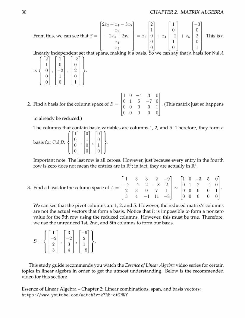
From this, we can see that ~x =
2x2 + x4 − 3x5
x2−2x4 + 2x5
x4x5
= x2
21000
+ x4
10−210
+ x5
−30201
. This is a
linearly independent set that spans, making it a basis. So we can say that a basis for NulA
is
21000
,
10−210
,−30201
.
2. Find a basis for the column space of B =
1 0 −4 3 00 1 5 −7 00 0 0 0 10 0 0 0 0
. (This matrix just so happens
to already be reduced.)
The columns that contain basic variables are columns 1, 2, and 5. Therefore, they form a
basis for ColB:
1000
,0100
,0010
.
Important note: The last row is all zeroes. However, just because every entry in the fourthrow is zero does not mean the entries are in R3; in fact, they are actually in R4.
3. Find a basis for the column space of A =
1 3 3 2 −9−2 −2 2 −8 22 3 0 7 13 4 −1 11 −8
∼1 0 −3 5 00 1 2 −1 00 0 0 0 10 0 0 0 0
.
We can see that the pivot columns are 1, 2, and 5. However, the reduced matrix’s columnsare not the actual vectors that form a basis. Notice that it is impossible to form a nonzerovalue for the 5th row using the reduced columns. However, this must be true. Therefore,we use the unreduced 1st, 2nd, and 5th columns to form our basis.
B =
1−223
,
3−234
,−921−8
.
This study guide recommends you watch the Essence of Linear Algebra video series for certaintopics in linear algebra in order to get the utmost understanding. Below is the recommendedvideo for this section:
Essence of Linear Algebra – Chapter 2: Linear combinations, span, and basis vectors:https://www.youtube.com/watch?v=k7RM-ot2NWY
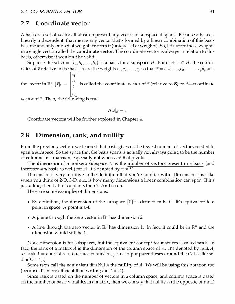
2.7. COORDINATE VECTOR 31
2.7 Coordinate vector
A basis is a set of vectors that can represent any vector in subspace it spans. Because a basis islinearly independent, that means any vector that’s formed by a linear combination of this basishas one and only one set of weights to form it (unique set of weights). So, let’s store these weightsin a single vector called the coordinate vector. The coordinate vector is always in relation to thisbasis, otherwise it wouldn’t be valid.
Suppose the set B = {~b1,~b2, . . . ,~bp} is a basis for a subspace H . For each ~x ∈ H , the coordi-nates of ~x relative to the basis ~B are the weights c1, c2, . . . , cp so that ~x = c1~b1+c2~b2+ · · ·+cp~bp and
the vector in Rp, [~x]B =
c1c2...cp
is called the coordinate vector of ~x (relative to B) or B—coordinate
vector of ~x. Then, the following is true:
B[~x]B = ~x
Coordinate vectors will be further explored in Chapter 4.
2.8 Dimension, rank, and nullity
From the previous section, we learned that basis gives us the fewest number of vectors needed tospan a subspace. So the space that the basis spans is actually not always going to be the numberof columns in a matrix n, especially not when n 6= # of pivots.
The dimension of a nonzero subspace H is the number of vectors present in a basis (andtherefore any basis as well) for H. It’s denoted by dimH .
Dimension is very intuitive to the definition that you’re familiar with. Dimension, just likewhen you think of 2-D, 3-D, etc., is how many dimensions a linear combination can span. If it’sjust a line, then 1. If it’s a plane, then 2. And so on.
Here are some examples of dimensions:
• By definition, the dimension of the subspace {~0} is defined to be 0. It’s equivalent to apoint in space. A point is 0-D.
• A plane through the zero vector in R3 has dimension 2.
• A line through the zero vector in R2 has dimension 1. In fact, it could be in Rn and thedimension would still be 1.
Now, dimension is for subspaces, but the equivalent concept for matrices is called rank. Infact, the rank of a matrix A is the dimension of the column space of A. It’s denoted by rankA,so rankA = dimColA. (To reduce confusion, you can put parentheses around the ColA like so:dim(ColA).)
Some texts call the equivalent dimNulA the nullity of A. We will be using this notation too(because it’s more efficient than writing dimNulA).
Since rank is based on the number of vectors in a column space, and column space is basedon the number of basic variables in a matrix, then we can say that nullityA (the opposite of rank)
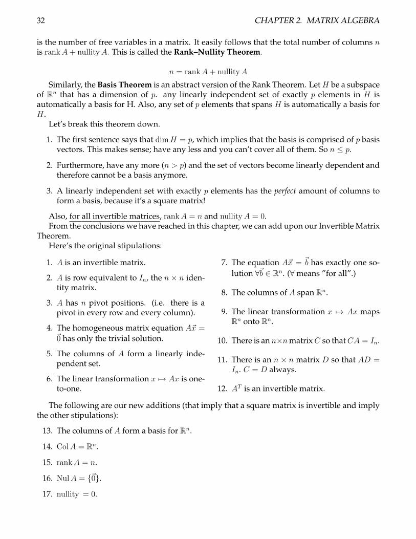
32 CHAPTER 2. MATRIX ALGEBRA
is the number of free variables in a matrix. It easily follows that the total number of columns nis rankA+ nullityA. This is called the Rank–Nullity Theorem.
n = rankA+ nullityA
Similarly, the Basis Theorem is an abstract version of the Rank Theorem. LetH be a subspaceof Rn that has a dimension of p. any linearly independent set of exactly p elements in H isautomatically a basis for H. Also, any set of p elements that spans H is automatically a basis forH .
Let’s break this theorem down.
1. The first sentence says that dimH = p, which implies that the basis is comprised of p basisvectors. This makes sense; have any less and you can’t cover all of them. So n ≤ p.
2. Furthermore, have any more (n > p) and the set of vectors become linearly dependent andtherefore cannot be a basis anymore.
3. A linearly independent set with exactly p elements has the perfect amount of columns toform a basis, because it’s a square matrix!
Also, for all invertible matrices, rankA = n and nullityA = 0.From the conclusions we have reached in this chapter, we can add upon our Invertible Matrix
Theorem.Here’s the original stipulations:
1. A is an invertible matrix.
2. A is row equivalent to In, the n × n iden-tity matrix.
3. A has n pivot positions. (i.e. there is apivot in every row and every column).
4. The homogeneous matrix equation A~x =~0 has only the trivial solution.
5. The columns of A form a linearly inde-pendent set.
6. The linear transformation x 7→ Ax is one-to-one.
7. The equation A~x = ~b has exactly one so-lution ∀~b ∈ Rn. (∀means ”for all”.)
8. The columns of A span Rn.
9. The linear transformation x 7→ Ax mapsRn onto Rn.
10. There is an n×nmatrixC so thatCA = In.
11. There is an n × n matrix D so that AD =In. C = D always.
12. AT is an invertible matrix.
The following are our new additions (that imply that a square matrix is invertible and implythe other stipulations):
13. The columns of A form a basis for Rn.
14. ColA = Rn.
15. rankA = n.
16. NulA = {~0}.
17. nullity = 0.
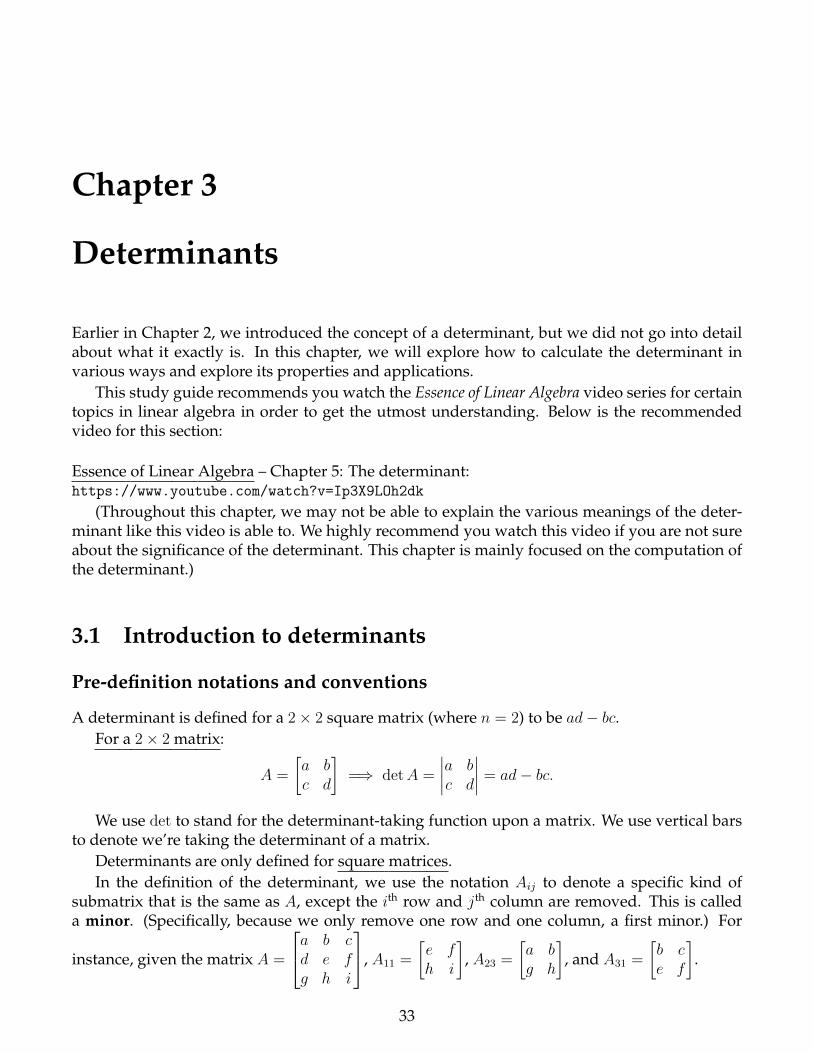
Chapter 3
Determinants
Earlier in Chapter 2, we introduced the concept of a determinant, but we did not go into detailabout what it exactly is. In this chapter, we will explore how to calculate the determinant invarious ways and explore its properties and applications.
This study guide recommends you watch the Essence of Linear Algebra video series for certaintopics in linear algebra in order to get the utmost understanding. Below is the recommendedvideo for this section:
Essence of Linear Algebra – Chapter 5: The determinant:https://www.youtube.com/watch?v=Ip3X9LOh2dk
(Throughout this chapter, we may not be able to explain the various meanings of the deter-minant like this video is able to. We highly recommend you watch this video if you are not sureabout the significance of the determinant. This chapter is mainly focused on the computation ofthe determinant.)
3.1 Introduction to determinants
Pre-definition notations and conventions
A determinant is defined for a 2× 2 square matrix (where n = 2) to be ad− bc.For a 2× 2 matrix:
A =
[a bc d
]=⇒ detA =
∣∣∣∣a bc d
∣∣∣∣ = ad− bc.
We use det to stand for the determinant-taking function upon a matrix. We use vertical barsto denote we’re taking the determinant of a matrix.
Determinants are only defined for square matrices.In the definition of the determinant, we use the notation Aij to denote a specific kind of
submatrix that is the same as A, except the ith row and jth column are removed. This is calleda minor. (Specifically, because we only remove one row and one column, a first minor.) For
instance, given the matrix A =
a b cd e fg h i
, A11 =
[e fh i
], A23 =
[a bg h
], and A31 =
[b ce f
].
33
34 CHAPTER 3. DETERMINANTS
Definition of the determinant
For cases where n ≥ 2, we define the determinant of an n× n matrix A = [aij] to be
detA = a11 detA11 − a12 detA12 + · · ·+ (−1)n−1a1n detA1n
=n∑
j=1
(−1)1+ja1j detA1j
Notice that the summation alternates signs on each successive term. This is represented by(−1)n−1.
This is the most common method to calculate a determinant. However, because this canget computationally heavy for larger matrices, we will now explore ways to more efficientlycalculate determinants.
Laplace expansion (cofactor expansion)
One way we can reduce the number of calculations is to select other rows or columns to act asminors. In the definition above, we only use the first row. There are many cases where the firstrow is not as efficient as using other rows. Whenever a row contains many zeroes, it will allowthe coefficient in the front to be zero, cancelling out that term. We want to do less work, so thisis desirable. In this case, we will calculate something called the cofactor and use a theorem calledLaplace expansion to calculate the determinant.
Given A = [aij], the (i, j)-cofactor of A is the number Cij and is:
Cij = (−1)i+j detAij
Using this cofactor definition, we can use a generalized formula for a determinant:
detA = a11C11 + a12C12 + · · ·+ a1nC1n
This formula is the cofactor expansion across the first row of A. What we have done is takethe original definition and squeeze detAij and the alternating sign term into Cij . But what aboutcalculating the cofactor expansion for any row or column? We shall use the Laplace expansiontheorem (cofactor expansion across any row or column):
The determinant of an n × n matrix A can be computed by a cofactor expansion across anyrow or down any column. For each 1 ≤ i ≤ n and 1 ≤ j ≤ n:
detA = ai1Ci1 + ai2Ci2 + · · ·+ ainCin (for rows)= a1jC1j + a2jC2j + · · ·+ anjCnj (for columns)
Keep in mind that the alternation of signs is now determined by the cofactor term!
Sign patterns for terms of a determinant summation
In the definition of a cofactor, the sign is determined by the term (−1)i+j . This means
• if i+ j is even, the term will be positive.
• if i+ j is odd, the term will be negative.
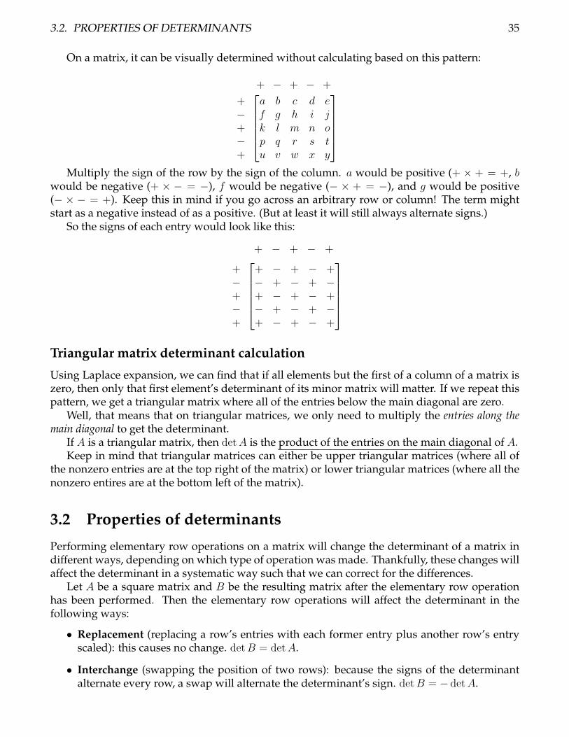
3.2. PROPERTIES OF DETERMINANTS 35
On a matrix, it can be visually determined without calculating based on this pattern:
+ − + − +
+−+−+
a b c d ef g h i jk l m n op q r s tu v w x y
Multiply the sign of the row by the sign of the column. a would be positive (+ × + = +, b
would be negative (+ × − = −), f would be negative (− × + = −), and g would be positive(− × − = +). Keep this in mind if you go across an arbitrary row or column! The term mightstart as a negative instead of as a positive. (But at least it will still always alternate signs.)
So the signs of each entry would look like this:
+ − + − +
+−+−+
+ − + − +− + − + −+ − + − +− + − + −+ − + − +
Triangular matrix determinant calculation
Using Laplace expansion, we can find that if all elements but the first of a column of a matrix iszero, then only that first element’s determinant of its minor matrix will matter. If we repeat thispattern, we get a triangular matrix where all of the entries below the main diagonal are zero.
Well, that means that on triangular matrices, we only need to multiply the entries along themain diagonal to get the determinant.
If A is a triangular matrix, then detA is the product of the entries on the main diagonal of A.Keep in mind that triangular matrices can either be upper triangular matrices (where all of
the nonzero entries are at the top right of the matrix) or lower triangular matrices (where all thenonzero entires are at the bottom left of the matrix).
3.2 Properties of determinants
Performing elementary row operations on a matrix will change the determinant of a matrix indifferent ways, depending on which type of operation was made. Thankfully, these changes willaffect the determinant in a systematic way such that we can correct for the differences.
Let A be a square matrix and B be the resulting matrix after the elementary row operationhas been performed. Then the elementary row operations will affect the determinant in thefollowing ways:
• Replacement (replacing a row’s entries with each former entry plus another row’s entryscaled): this causes no change. detB = detA.
• Interchange (swapping the position of two rows): because the signs of the determinantalternate every row, a swap will alternate the determinant’s sign. detB = − detA.

36 CHAPTER 3. DETERMINANTS
• Scaling (multiplying all of the entries of a row by a scalar): if you multiplied a row by k,then the new determinant is k times the old determinant. detB = k detA.
Caution! When performing row operations, we really are doing detA → 1kdetB. Keep in
mind the difference between the definition of scaling and how it is applied in row reduction.Another property is relating the numerical value of the determinant with the actual invert-
ibility of the matrix. If a matrix’s determinant is zero, it is singular (i.e. not invertible). If it’snonzero, it’s invertible. If the determinant function is not defined, then it’s not a square matrix.
detA = 0 ⇐⇒ A is singular
The determinant of a matrix’s transpose is the same as the original matrix. Therefore, we canactually perform ”elementary column operations” on a matrix and get the same determinant.
detA = detAT
One last property is that:
det(AB) = (detA)(detB)
Summary of determinant properties
• Replacement: detB = detA
• Interchange: detB = − detA
• Scaling: detB = k detA
• detA 6= 0 ⇐⇒ A invertible
• detA = detAT
• det(AB) = (detA)(detB)
3.3 Cramer’s rule
For the matrix equation A~x = ~b, you can solve for each of ~x’s entries xi by using Cramer’s rule.While it is computationally ineffective, it works. Let Ai(~b) be the matrix A but the ith column isreplaced with~b. Then the ith entry of ~x can be determined with the following formula:
xi =detAi(~b)
detA
Chapter 4
Vector spaces
Vector spaces are an abstract concept that’s similar to a subspace, which we defined earlier. Infact, this is where linear algebra ties into abstract algebra, which is a higher-order class of algebra.In this chapter, we’ll link everything we have learned so far with this more general concept ofvector spaces, and introduce some new, pertinent things along the way.
4.1 Introduction to vector spaces and their relation to subspaces
An integral part of abstract algebra is grouping structures, each with its own unique character-istics. A vector space is a kind of structure; it’s a nonempty set (let’s call it V ) of objects (calledvectors) on which are defined two operations: addition and scalar multiplication. Vector spacesare subject to the following axioms that make vector spaces what they are:
1. Just like subspaces, V is closed under ad-dition. That means adding two vectors inV will always produce a vector that’s stillin V .
2. V is also closed under scalar multiplica-tion.
3. The addition operation is communica-tive: ~u+~v = ~v+~u - it doesn’t matter whichoperand (~u and ~v are operands) comesfirst.
4. The addition operation is associative. (~u+~v) + ~w = ~u+ (~v + ~w) - it doesn’t matter inwhich order you process the operations.
5. There is a zero vector~0 ∈ V so that ~u+~0 =~u. (In abstract algebra, this is known asthe identity element.)
6. For each ~u ∈ V , there is a vector −~u ∈ Vso that ~u+ (−~u) = ~0.
7. The scalar multiplication operation is dis-tributive. c(~u+~v) = c~u+c~v and (c+d)~u =c~u+ d~u.
8. The scalar multiplication operation is as-sociative. c(d~u) = (cd)~u.
9. The identity property for scalar multipli-cation is that 1~u = ~u.
Where do vector spaces come in? Previously, when we defined linear transformations, wewere actually being too specific on what space it occurred in. A linear mapping is a transforma-tion from one vector space to another. So that means working with vector spaces is like workingin Rn: now, instead of using Rn, we use vector spaces and all the properties that come with it. (Infact, an n-dimensional vector space is an isomorphism of Rn — i.e. it is a one-to-one mapping.)
The following are vector spaces:
37
38 CHAPTER 4. VECTOR SPACES
• Mm,n, the set ofm×nmatrices, whose en-tries are in R.
• Mn, the set of all n × n matrices, whoseentries are in R.
• Rn.
• Pn – polynomials of at most degree n invariable x with coefficients in the reals(R).
• P∞ – power series in x of the form∞∑n=0
anxn.
• Let S be the set of doubly infinite se-quences, {y} = (. . . , y−2, y−1, y0, y1, y2, . . . ).
• Let F = {f : R 7→ R} be the set of real-valued functions with operations (f +g)(x) = f(x)+ g(x) and (rf)(x) = r · f(x).
Subspaces in relation to vector spaces
We already defined what a subspace is. Now, we can say that subspaces are really just vectorspaces living in other vector spaces. They exist in other vector spaces. It’s like a house within ahouse.
Which of the following are subspaces? Let’s use the definition we established back in Chapter2.
• {~0} in a vector space V ? Yes.
• Pn ⊂ P∞? Yes.
• Invertible n× n matrices in Mn? Well, thezero matrix has no pivots. Furthermore,neither matrix addition nor matrix multi-plication are closed operations. No.
• Upper triangular matrices n × n in Mn?Zero matrix is technically an upper trian-gular matrix. And it’s closed under addi-tion and scalar multiplication. Yes.
• Is R2 a subspace of R3? No, they’re con-sidered entirely different subspaces. Youcan’t add something in R2 to R3. No.
• Is H = {
rs0
: r, s ∈ R} a subspace of
R3? Isomorphisms (which we have notdefined yet) has that zero, but it has 3 en-tries, so it’s in R3. Yes.
• A line not through the origin in R2, or aplane not through the origin in R3? Theydo not include their respective zero vec-tors. No.
• The set of all points in the form (3s, 2+5s)in R2? That additive factor makes thezero vector outside of this set. No.
Now, subspaces are simply parts of a vector space. For instance, a plane going through theorigin in R3 would be considered a subspace of R3. (We will later establish that Rn is effectivelya vector space.)
Now, how do we create subspaces? We usually start with linear combinations. It turns outthat the following theorem provides a good foundation:
If ~v1, ~v2, . . . , ~vp are vectors in a vector space V , then Span{~v1, ~v2, . . . , ~vp} is a subspace of V .This is basically saying that you can use some vectors in a specific vector space to form a
linear combination, and all the possible combinations creates a subspace of the vector space thevectors were in.
The easiest way to show something is a subspace of a space is to show it is a spanning setof a space. We call Span{~v1, ~v2, . . . , ~vp} the subspace spanned by (or generated by) ~v1, ~v2, . . . , ~vp.Given a subspace H of V , a spanning set (or generating set) of H is a set {~v1, ~v2, . . . , ~vp} so thatH = Span{~v1, ~v2, . . . , ~vp}.
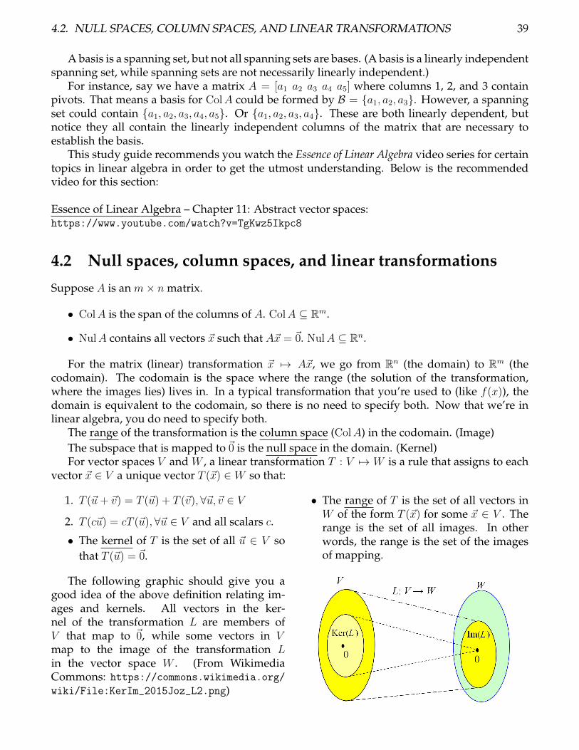
4.2. NULL SPACES, COLUMN SPACES, AND LINEAR TRANSFORMATIONS 39
A basis is a spanning set, but not all spanning sets are bases. (A basis is a linearly independentspanning set, while spanning sets are not necessarily linearly independent.)
For instance, say we have a matrix A = [a1 a2 a3 a4 a5] where columns 1, 2, and 3 containpivots. That means a basis for ColA could be formed by B = {a1, a2, a3}. However, a spanningset could contain {a1, a2, a3, a4, a5}. Or {a1, a2, a3, a4}. These are both linearly dependent, butnotice they all contain the linearly independent columns of the matrix that are necessary toestablish the basis.
This study guide recommends you watch the Essence of Linear Algebra video series for certaintopics in linear algebra in order to get the utmost understanding. Below is the recommendedvideo for this section:
Essence of Linear Algebra – Chapter 11: Abstract vector spaces:https://www.youtube.com/watch?v=TgKwz5Ikpc8
4.2 Null spaces, column spaces, and linear transformations
Suppose A is an m× n matrix.
• ColA is the span of the columns of A. ColA ⊆ Rm.
• NulA contains all vectors ~x such that A~x = ~0. NulA ⊆ Rn.
For the matrix (linear) transformation ~x 7→ A~x, we go from Rn (the domain) to Rm (thecodomain). The codomain is the space where the range (the solution of the transformation,where the images lies) lives in. In a typical transformation that you’re used to (like f(x)), thedomain is equivalent to the codomain, so there is no need to specify both. Now that we’re inlinear algebra, you do need to specify both.
The range of the transformation is the column space (ColA) in the codomain. (Image)The subspace that is mapped to ~0 is the null space in the domain. (Kernel)For vector spaces V and W , a linear transformation T : V 7→ W is a rule that assigns to each
vector ~x ∈ V a unique vector T (~x) ∈ W so that:
1. T (~u+ ~v) = T (~u) + T (~v),∀~u,~v ∈ V
2. T (c~u) = cT (~u),∀~u ∈ V and all scalars c.
• The kernel of T is the set of all ~u ∈ V sothat T (~u) = ~0.
• The range of T is the set of all vectors inW of the form T (~x) for some ~x ∈ V . Therange is the set of all images. In otherwords, the range is the set of the imagesof mapping.
The following graphic should give you agood idea of the above definition relating im-ages and kernels. All vectors in the ker-nel of the transformation L are members ofV that map to ~0, while some vectors in Vmap to the image of the transformation Lin the vector space W . (From WikimediaCommons: https://commons.wikimedia.org/wiki/File:KerIm_2015Joz_L2.png)
40 CHAPTER 4. VECTOR SPACES
4.3 Spanning sets
If we have a set of vectors S that are able to span all vectors in a vector space V , then we call S aspanning set. In contrast to a basis, a spanning set may not necessarily be linearly independent(i.e. there may be redundant vectors in it).
Two important stipulations arise from a spanning set:
1. If some ~vk ∈ S is a linear combination of the remaining vectors in S (i.e. it’s redundant),then S is linearly dependent because of ~vk, so the set S ′ formed by removing ~vk still spans~vk.
2. If H is not simply the zero vector (H 6= {~0}), then some subset of S is a basis for H . (Fromthis spanning set, if we take some or all of the vectors from it, it’ll form a basis.)
4.4 Coordinate systems
In this section, we will learn that since bases are unique representations for the vectors that itspans, we can simply take a vector containing relevant weights (i.e. a coordinate vector), withtheir order corresponding with the vectors in a basis, and multiplying them together will returnthat same vector ~x.
Remember from chapter 2, we established what a coordinate vector was. Now we extendthis to vector spaces too: If we have a basis B = {~b1,~b2, . . . ,~bn} which is a basis for vector spaceV , then for each vector in V (~x ∈ V ), there’s a unique set of scalars c1, c2, . . . , cn (weights) so thatwhen they’re combined with their respective basis vectors, they form ~x.
~x = c1~b1 + c2~b2 + · · ·+ cn~bn
Not only do these weights exist, but these weights are unique. This means using this spe-cific basis, there is only one set of scalars to represent ~x. This is the stipulation of the uniquerepresentation theorem.
A vector that stores these unique weights, as we have established in chapter 2, is called acoordinate vector. It turns out that we can transform our vector ~x into the coordinate vectorrelative to a certain basis. The linear transformation ~x 7→ [~x]B is called the coordinate mappingdetermined by B. This allows the following to be true:
PB[~x]B = ~x
where PB =[~b1 ~b2 . . . ~bn
], the matrix whose columns comprise of the basis vectors in B.
Fun fact: Under the standard basis E = {~e1, ~e2}, which comprise the columns of the identitymatrix I , all coordinate vectors are equivalent to the vectors they form with the standard basisE .
This linear transformation ~x 7→ [~x]B is one-to-one and onto. Everything in vector space V(which is where ~x resides) also exists on W (which is where [~x]B resides). That means this trans-formation is easily reversible, and all operations for V are also applicable to W when trans-formed accordingly.
When we have a one-to-one transformation from V onto W , we call this an isomorphism. Iftwo vector spaces have an isomorphism between them, they’re isomorphic.
4.5. DIMENSION OF A VECTOR SPACE 41
Isomorphisms provide immense benefits. We can now relate each and every vector operationand calculation in V to those in W .
• Since isomorphisms are one-to-one and onto, they are invertible.
• Since they are linear transformations, we can work with [~x]B in Rn the same way we workwith ~x in V . Vector spaces isomorphic to each other are functionally the same space. Wecan therefore relate these vector spaces with Rn.
We have now established that we can extend this relationship not just between vector spaces,but also from a vector space to Rn. If a basis B = {~b1,~b2, . . . ,~bn} for the vector space V hasa coordinate mapping ~x 7→ [~x]B, then this mapping is one-to-one from V onto Rn. (i.e. themapping is an isomorphism between V and Rn.)
V ' Rn
For instance, if we are given a basis B =
362
,−10
1
for a subspace H , and we want to
see whether ~x =
3127
∈ H . If so, find [~x]B.
Reducing the augmented matrix [~v1~v2|~x] gives us
3 −1 36 0 122 1 7
∼1 0 20 1 30 0 0
. Since this matrix
is consistent, we can establish ~x ∈ H . Furthermore, we can see that x1 = 2 and x2 = 3, so the
coordinate vector relative to basis B is [~x]B =[23
]. Note that there isn’t a x3 variable. This means
the coordinate vector is in R2 even though the basis vectors and ~x are in R3.What can we conclude from this example? The dimension of H is 2, aka dimH = 2, because
there are only two entries in the coordinate vector. Furthermore, this establishes H ' R2 (H isisomorphic to R2 but living in R3).
In R3, any subspace H will have either dimension 0, 1, 2, or 3. If dimH = 1, then this is acopy of R in R3 (an isomorphism). H ' R but H ⊆ R3.
4.5 Dimension of a vector space
We can generalize the definition of linear independence to vector spaces too, and use this to formthe definition of a dimension space of a vector space. Below are some fundamental theorems andfacts concerning this subject matter.
1. Let’s say a vector space V has a basis B = {~b1,~b2, . . . ,~bn}. Then any set in V more than nvectors must necessarily be linearly dependent.
2. If a vector space V has a basis of n vectors, then every basis of the same V must also containexactly n vectors.
This makes sense. Otherwise, if there are any fewer, it would only be able to span a certainsubspace of V , but not all of V . If there were more vectors and all were still linearly inde-pendent, then that’s an even larger V . But if there were more vectors and the newly added
42 CHAPTER 4. VECTOR SPACES
vector were linearly dependent to the original set, then that’s not a basis anymore (sinceit’s not linearly independent), only a spanning set.
3. If V is not spanned by a finite set, then V is infinite-dimensional.
4. If H is a subspace of a finite-dimensional vector space V , then any linearly independentset in H can become a basis of H if necessary. Also, H will be finite-dimensional anddimH ≤ dimV .
5. Basis Theorem: If V is a p-dimensional vector space (where p ≥ 1), then any linearly inde-pendent set of exactly p elements in V is automatically a basis for V . Any set of exactly pelements that spans V is also automatically a basis for V .
This means we can show that two vector spaces are the exact same thing if they have thesame span. For instance, let’s say we have a 3×7 matrixAwith 3 pivots. Is its column spaceequal to R3? Usually, the answer would be no. However, we need to carefully consider thiscase. We know that ColA ⊆ R3 (it’s definitely a subspace of R3). But we also know there’s3 pivots in the matrix. This means the dimension of the column space (or rank) is 3. Thedimension of R3 is also 3. Since they have the same dimension, coupled with the fact thatColA is a subspace of R3, we can therefore conclude ColA = R3.
4.6 Rank of a vector space’s matrix
We can carry over the same definitions from Chapter 2 over what a rank of R2 is, and now applyit to any vector space V through isomorphisms. Now, let’s introduce a new concept called a rowspace. It’s the set of the possible linear combinations of the rows (instead of columns) of a matrixA. The row space of A is equivalent to the column space of A transpose.
RowA = ColAT
Finding a basis for our row space RowA is easy. Simply row reduceA to reduced row echelonform. Then use the nonzero rows of the reduced row echelon matrix (i.e. the ones with pivots,or pivot rows) to form your basis.
While the row space of A is the same as A reduced, it is important to note that you cannotalways use the rows of A unreduced to form a basis for RowA. You should only use the rows ofA reduced to form the basis, but knowing that they are the same because row reductions do notaffect the row space.
In fact, let’s generalize the sharing of row spaces: if two matricesA andB are row equivalent,then their row spaces are actually equivalent. If B is in reduced echelon form, the nonzero rowsof B will form a basis for both RowA and RowB. (This means all invertible matrices have thesame row space.)
A ∼ B =⇒ RowA = RowB
Furthermore, because there are the same number of pivot columns and pivot rows, we canconclude that the dimension of the column space (rankA) is equivalent to the dimension of therow space.
rankA = dimColA = dimRowA
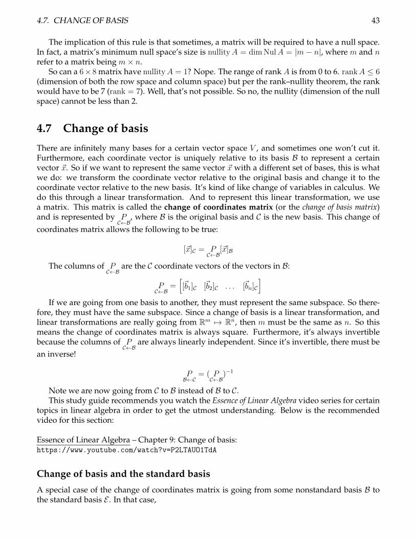
4.7. CHANGE OF BASIS 43
The implication of this rule is that sometimes, a matrix will be required to have a null space.In fact, a matrix’s minimum null space’s size is nullityA = dimNulA = |m − n|, where m and nrefer to a matrix being m× n.
So can a 6× 8 matrix have nullityA = 1? Nope. The range of rank A is from 0 to 6. rankA ≤ 6(dimension of both the row space and column space) but per the rank–nullity theorem, the rankwould have to be 7 (rank = 7). Well, that’s not possible. So no, the nullity (dimension of the nullspace) cannot be less than 2.
4.7 Change of basis
There are infinitely many bases for a certain vector space V , and sometimes one won’t cut it.Furthermore, each coordinate vector is uniquely relative to its basis B to represent a certainvector ~x. So if we want to represent the same vector ~x with a different set of bases, this is whatwe do: we transform the coordinate vector relative to the original basis and change it to thecoordinate vector relative to the new basis. It’s kind of like change of variables in calculus. Wedo this through a linear transformation. And to represent this linear transformation, we usea matrix. This matrix is called the change of coordinates matrix (or the change of basis matrix)and is represented by P
C←B, where B is the original basis and C is the new basis. This change of
coordinates matrix allows the following to be true:
[~x]C = PC←B
[~x]B
The columns of PC←B
are the C coordinate vectors of the vectors in B:
PC←B
=[[~b1]C [~b2]C . . . [~bn]C
]If we are going from one basis to another, they must represent the same subspace. So there-
fore, they must have the same subspace. Since a change of basis is a linear transformation, andlinear transformations are really going from Rm 7→ Rn, then m must be the same as n. So thismeans the change of coordinates matrix is always square. Furthermore, it’s always invertiblebecause the columns of P
C←Bare always linearly independent. Since it’s invertible, there must be
an inverse!
PB←C
= ( PC←B
)−1
Note we are now going from C to B instead of B to C.This study guide recommends you watch the Essence of Linear Algebra video series for certain
topics in linear algebra in order to get the utmost understanding. Below is the recommendedvideo for this section:
Essence of Linear Algebra – Chapter 9: Change of basis:https://www.youtube.com/watch?v=P2LTAUO1TdA
Change of basis and the standard basis
A special case of the change of coordinates matrix is going from some nonstandard basis B tothe standard basis E . In that case,
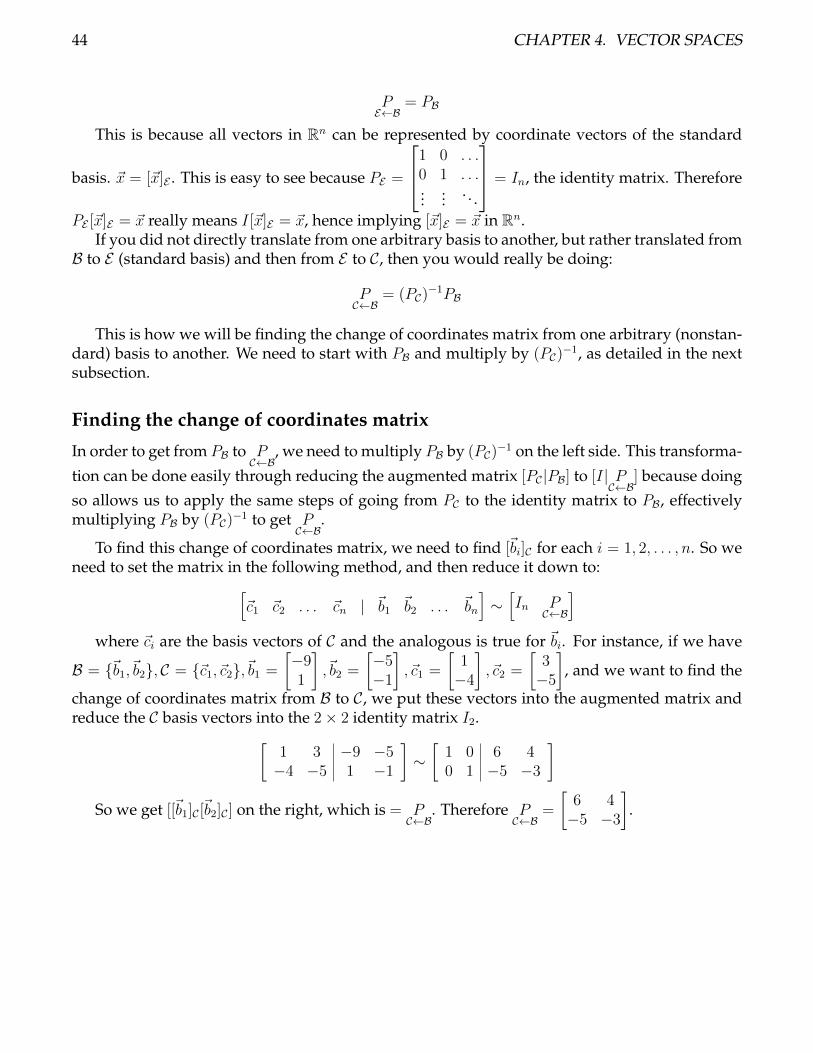
44 CHAPTER 4. VECTOR SPACES
PE←B
= PB
This is because all vectors in Rn can be represented by coordinate vectors of the standard
basis. ~x = [~x]E . This is easy to see because PE =
1 0 . . .0 1 . . ....
... . . .
= In, the identity matrix. Therefore
PE [~x]E = ~x really means I[~x]E = ~x, hence implying [~x]E = ~x in Rn.If you did not directly translate from one arbitrary basis to another, but rather translated from
B to E (standard basis) and then from E to C, then you would really be doing:
PC←B
= (PC)−1PB
This is how we will be finding the change of coordinates matrix from one arbitrary (nonstan-dard) basis to another. We need to start with PB and multiply by (PC)
−1, as detailed in the nextsubsection.
Finding the change of coordinates matrix
In order to get from PB to PC←B
, we need to multiply PB by (PC)−1 on the left side. This transforma-
tion can be done easily through reducing the augmented matrix [PC|PB] to [I| PC←B
] because doing
so allows us to apply the same steps of going from PC to the identity matrix to PB, effectivelymultiplying PB by (PC)
−1 to get PC←B
.
To find this change of coordinates matrix, we need to find [~bi]C for each i = 1, 2, . . . , n. So weneed to set the matrix in the following method, and then reduce it down to:[
~c1 ~c2 . . . ~cn | ~b1 ~b2 . . . ~bn
]∼[In P
C←B
]where ~ci are the basis vectors of C and the analogous is true for ~bi. For instance, if we have
B = {~b1,~b2}, C = {~c1,~c2},~b1 =
[−91
],~b2 =
[−5−1
],~c1 =
[1−4
],~c2 =
[3−5
], and we want to find the
change of coordinates matrix from B to C, we put these vectors into the augmented matrix andreduce the C basis vectors into the 2× 2 identity matrix I2.[
1 3 −9 −5−4 −5 1 −1
]∼[1 0 6 40 1 −5 −3
]So we get [[~b1]C[~b2]C] on the right, which is = P
C←B. Therefore P
C←B=
[6 4−5 −3
].
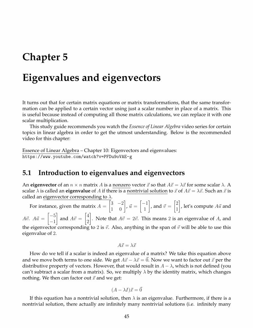
Chapter 5
Eigenvalues and eigenvectors
It turns out that for certain matrix equations or matrix transformations, that the same transfor-mation can be applied to a certain vector using just a scalar number in place of a matrix. Thisis useful because instead of computing all those matrix calculations, we can replace it with onescalar multiplication.
This study guide recommends you watch the Essence of Linear Algebra video series for certaintopics in linear algebra in order to get the utmost understanding. Below is the recommendedvideo for this chapter:
Essence of Linear Algebra – Chapter 10: Eigenvectors and eigenvalues:https://www.youtube.com/watch?v=PFDu9oVAE-g
5.1 Introduction to eigenvalues and eigenvectors
An eigenvector of an n× n matrix A is a nonzero vector ~x so that A~x = λ~x for some scalar λ. Ascalar λ is called an eigenvalue of A if there is a nontrivial solution to ~x of A~x = λ~x. Such an ~x iscalled an eigenvector corresponding to λ.
For instance, given the matrix A =
[3 −21 0
], ~u =
[−11
], and ~v =
[21
], let’s compute A~u and
A~v. A~u =
[−5−1
]and A~v =
[42
]. Note that A~v = 2~v. This means 2 is an eigenvalue of A, and
the eigenvector corresponding to 2 is ~v. Also, anything in the span of ~v will be able to use thiseigenvalue of 2.
A~x = λ~x
How do we tell if a scalar is indeed an eigenvalue of a matrix? We take this equation aboveand we move both terms to one side. We get A~x− λ~x = ~0. Now we want to factor out ~x per thedistributive property of vectors. However, that would result in A− λ, which is not defined (youcan’t subtract a scalar from a matrix). So, we multiply λ by the identity matrix, which changesnothing. We then can factor out ~x and we get:
(A− λI)~x = ~0
If this equation has a nontrivial solution, then λ is an eigenvalue. Furthermore, if there is anontrivial solution, there actually are infinitely many nontrivial solutions (i.e. infinitely many
45
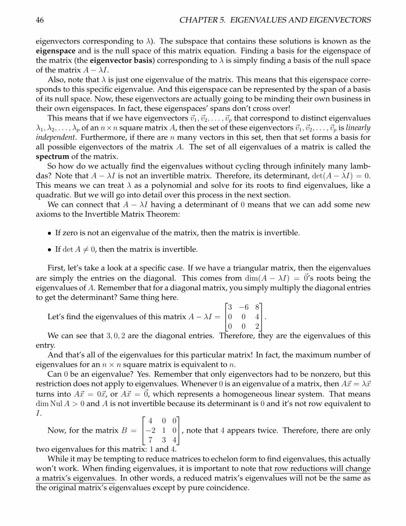
46 CHAPTER 5. EIGENVALUES AND EIGENVECTORS
eigenvectors corresponding to λ). The subspace that contains these solutions is known as theeigenspace and is the null space of this matrix equation. Finding a basis for the eigenspace ofthe matrix (the eigenvector basis) corresponding to λ is simply finding a basis of the null spaceof the matrix A− λI .
Also, note that λ is just one eigenvalue of the matrix. This means that this eigenspace corre-sponds to this specific eigenvalue. And this eigenspace can be represented by the span of a basisof its null space. Now, these eigenvectors are actually going to be minding their own business intheir own eigenspaces. In fact, these eigenspaces’ spans don’t cross over!
This means that if we have eigenvectors ~v1, ~v2, . . . , ~vp that correspond to distinct eigenvaluesλ1, λ2, . . . , λp of an n×n square matrixA, then the set of these eigenvectors ~v1, ~v2, . . . , ~vp is linearlyindependent. Furthermore, if there are n many vectors in this set, then that set forms a basis forall possible eigenvectors of the matrix A. The set of all eigenvalues of a matrix is called thespectrum of the matrix.
So how do we actually find the eigenvalues without cycling through infinitely many lamb-das? Note that A − λI is not an invertible matrix. Therefore, its determinant, det(A− λI) = 0.This means we can treat λ as a polynomial and solve for its roots to find eigenvalues, like aquadratic. But we will go into detail over this process in the next section.
We can connect that A − λI having a determinant of 0 means that we can add some newaxioms to the Invertible Matrix Theorem:
• If zero is not an eigenvalue of the matrix, then the matrix is invertible.
• If detA 6= 0, then the matrix is invertible.
First, let’s take a look at a specific case. If we have a triangular matrix, then the eigenvaluesare simply the entries on the diagonal. This comes from dim(A − λI) = ~0’s roots being theeigenvalues ofA. Remember that for a diagonal matrix, you simply multiply the diagonal entriesto get the determinant? Same thing here.
Let’s find the eigenvalues of this matrix A− λI =
3 −6 80 0 40 0 2
.
We can see that 3, 0, 2 are the diagonal entries. Therefore, they are the eigenvalues of thisentry.
And that’s all of the eigenvalues for this particular matrix! In fact, the maximum number ofeigenvalues for an n× n square matrix is equivalent to n.
Can 0 be an eigenvalue? Yes. Remember that only eigenvectors had to be nonzero, but thisrestriction does not apply to eigenvalues. Whenever 0 is an eigenvalue of a matrix, thenA~x = λ~x
turns into A~x = 0~x, or A~x = ~0, which represents a homogeneous linear system. That meansdimNulA > 0 and A is not invertible because its determinant is 0 and it’s not row equivalent toI .
Now, for the matrix B =
4 0 0−2 1 07 3 4
, note that 4 appears twice. Therefore, there are only
two eigenvalues for this matrix: 1 and 4.While it may be tempting to reduce matrices to echelon form to find eigenvalues, this actually
won’t work. When finding eigenvalues, it is important to note that row reductions will changea matrix’s eigenvalues. In other words, a reduced matrix’s eigenvalues will not be the same asthe original matrix’s eigenvalues except by pure coincidence.
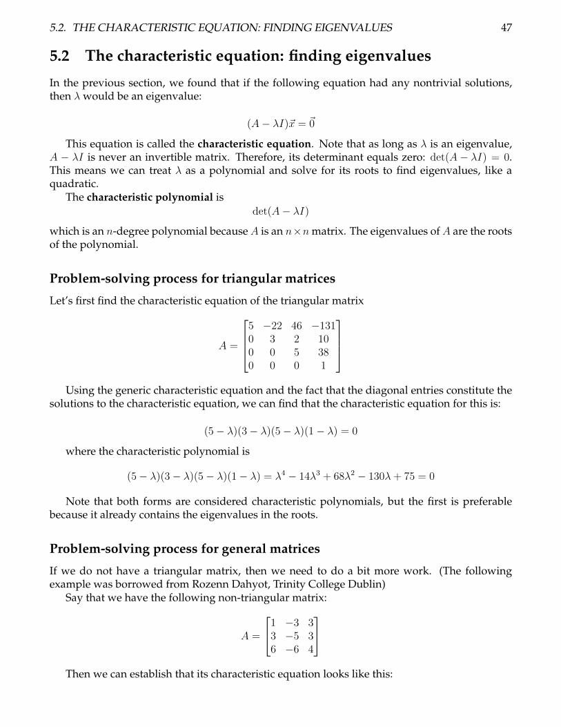
5.2. THE CHARACTERISTIC EQUATION: FINDING EIGENVALUES 47
5.2 The characteristic equation: finding eigenvalues
In the previous section, we found that if the following equation had any nontrivial solutions,then λ would be an eigenvalue:
(A− λI)~x = ~0
This equation is called the characteristic equation. Note that as long as λ is an eigenvalue,A − λI is never an invertible matrix. Therefore, its determinant equals zero: det(A− λI) = 0.This means we can treat λ as a polynomial and solve for its roots to find eigenvalues, like aquadratic.
The characteristic polynomial isdet(A− λI)
which is an n-degree polynomial becauseA is an n×nmatrix. The eigenvalues ofA are the rootsof the polynomial.
Problem-solving process for triangular matrices
Let’s first find the characteristic equation of the triangular matrix
A =
5 −22 46 −1310 3 2 100 0 5 380 0 0 1
Using the generic characteristic equation and the fact that the diagonal entries constitute the
solutions to the characteristic equation, we can find that the characteristic equation for this is:
(5− λ)(3− λ)(5− λ)(1− λ) = 0
where the characteristic polynomial is
(5− λ)(3− λ)(5− λ)(1− λ) = λ4 − 14λ3 + 68λ2 − 130λ+ 75 = 0
Note that both forms are considered characteristic polynomials, but the first is preferablebecause it already contains the eigenvalues in the roots.
Problem-solving process for general matrices
If we do not have a triangular matrix, then we need to do a bit more work. (The followingexample was borrowed from Rozenn Dahyot, Trinity College Dublin)
Say that we have the following non-triangular matrix:
A =
1 −3 33 −5 36 −6 4
Then we can establish that its characteristic equation looks like this:
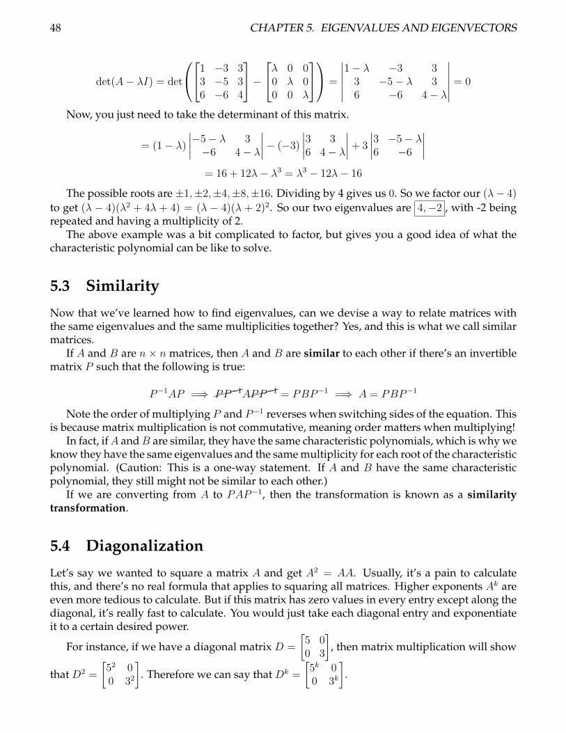
48 CHAPTER 5. EIGENVALUES AND EIGENVECTORS
det(A− λI) = det
1 −3 33 −5 36 −6 4
−λ 0 00 λ 00 0 λ
=
∣∣∣∣∣∣1− λ −3 33 −5− λ 36 −6 4− λ
∣∣∣∣∣∣ = 0
Now, you just need to take the determinant of this matrix.
= (1− λ)∣∣∣∣−5− λ 3−6 4− λ
∣∣∣∣− (−3)∣∣∣∣3 36 4− λ
∣∣∣∣+ 3
∣∣∣∣3 −5− λ6 −6
∣∣∣∣= 16 + 12λ− λ3 = λ3 − 12λ− 16
The possible roots are ±1,±2,±4,±8,±16. Dividing by 4 gives us 0. So we factor our (λ− 4)
to get (λ − 4)(λ2 + 4λ + 4) = (λ − 4)(λ + 2)2. So our two eigenvalues are 4,−2 , with -2 beingrepeated and having a multiplicity of 2.
The above example was a bit complicated to factor, but gives you a good idea of what thecharacteristic polynomial can be like to solve.
5.3 Similarity
Now that we’ve learned how to find eigenvalues, can we devise a way to relate matrices withthe same eigenvalues and the same multiplicities together? Yes, and this is what we call similarmatrices.
If A and B are n × n matrices, then A and B are similar to each other if there’s an invertiblematrix P such that the following is true:
P−1AP =⇒ ����PP−1A����
PP−1 = PBP−1 =⇒ A = PBP−1
Note the order of multiplying P and P−1 reverses when switching sides of the equation. Thisis because matrix multiplication is not commutative, meaning order matters when multiplying!
In fact, ifA andB are similar, they have the same characteristic polynomials, which is why weknow they have the same eigenvalues and the same multiplicity for each root of the characteristicpolynomial. (Caution: This is a one-way statement. If A and B have the same characteristicpolynomial, they still might not be similar to each other.)
If we are converting from A to PAP−1, then the transformation is known as a similaritytransformation.
5.4 Diagonalization
Let’s say we wanted to square a matrix A and get A2 = AA. Usually, it’s a pain to calculatethis, and there’s no real formula that applies to squaring all matrices. Higher exponents Ak areeven more tedious to calculate. But if this matrix has zero values in every entry except along thediagonal, it’s really fast to calculate. You would just take each diagonal entry and exponentiateit to a certain desired power.
For instance, if we have a diagonal matrix D =
[5 00 3
], then matrix multiplication will show
that D2 =
[52 00 32
]. Therefore we can say that Dk =
[5k 00 3k
].

5.4. DIAGONALIZATION 49
Furthermore, calculating eigenvalues from those non-triangular matrices is a pain. But it’sreally easy for diagonal matrices, because it’s just the values along the main diagonal. So whydon’t we find a way to relate those painful matrices to diagonal matrices?
We’ll use our similarity definition for diagonalization. A square matrix A is diagonalizableif and only if for some invertible P , it is similar to a diagonal matrix D and the following is true:
A = PDP−1
We can also rewrite this equation as
AP = PD
for computational ease so we can avoid finding the inverse of P .Also, from our realization that diagonal matrices are a great way to compute Ak, we can
conclude that:
Ak = PDkP−1
Now, let’s see an example of a A = PDP−1 equation:[7 2−4 1
]=
[1 1−1 −2
] [5 00 3
] [2 1−1 −1
]It turns out that an n × n matrix will only be diagonalizable if and only if A has n linearly-
independent eigenvectors. Thus, A is diagonalizable if and only if there are n vectors in theeigenvector basis, meaning it spans all of Rn. The columns of P actually comprise an eigenvectorbasis. The ith column of P corresponds to the entry dii (ith diagonal entry of D).
• The ith diagonal entry in D is an eigen-value of A.
• The ith column of P is the eigenvalue’scorresponding eigenvector.
• D’s diagonal entries are the spectrum ofA.
• P ’s columns comprise an eigenvector ba-sis relative to the eigenvalues in D.
So in the above example A = PDP−1 equation, 5 is one eigenvalue of A with corresponding
eigenvector[1−1
]and 3 is the other eigenvalue of A with corresponding eigenvector
[1−2
].
The process of diagonalizing matrices
Diagonalizing matrices can be done in six steps.
1. Find the eigenvalues of A.
2. Find the eigenvectors of A using theeigenvalues.
3. Check if there are n many eigenvectors.
4. Check whether they are all linearly inde-
pendent.
5. Assemble P using the eigenvectors youfound in step 2.
6. Create D using the eigenvalues youfound in step 1.
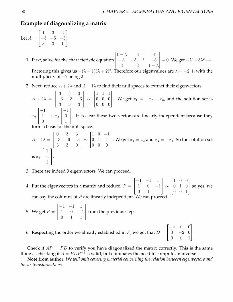
50 CHAPTER 5. EIGENVALUES AND EIGENVECTORS
Example of diagonalizing a matrix
Let A =
1 3 3−3 −5 −33 3 1
.
1. First, solve for the characteristic equation
∣∣∣∣∣∣1− λ 3 3−3 −5− λ −33 3 1− λ
∣∣∣∣∣∣ = 0. We get−λ3−3λ2+4.
Factoring this gives us −(λ− 1)(λ+ 2)2. Therefore our eigenvalues are λ = −2, 1, with themultiplicity of −2 being 2.
2. Next, reduce A+ 2λ and A− 1λ to find their null spaces to extract their eigenvectors.
A + 2λ =
3 3 3−3 −3 −33 3 3
∼1 1 10 0 00 0 0
. We get x1 = −x2 − x3, and the solution set is
x2
−110
+ x3
−101
. It is clear these two vectors are linearly independent because they
form a basis for the null space.
A− 1λ =
0 3 3−3 −6 −33 3 0
∼1 0 −10 1 10 0 0
. We get x1 = x3 and x2 = −x3. So the solution set
is x3
1−11
.
3. There are indeed 3 eigenvectors. We can proceed.
4. Put the eigenvectors in a matrix and reduce. P =
−1 −1 11 0 −10 1 1
∼1 0 00 1 00 0 1
so yes, we
can say the columns of P are linearly independent. We can proceed.
5. We get P =
−1 −1 11 0 −10 1 1
from the previous step.
6. Respecting the order we already established in P , we get that D =
−2 0 00 −2 00 0 1
.
Check if AP = PD to verify you have diagonalized the matrix correctly. This is the samething as checking if A = PDP−1 is valid, but eliminates the need to compute an inverse.
Note from author: We will omit covering material concerning the relation between eigenvectors andlinear transformations.
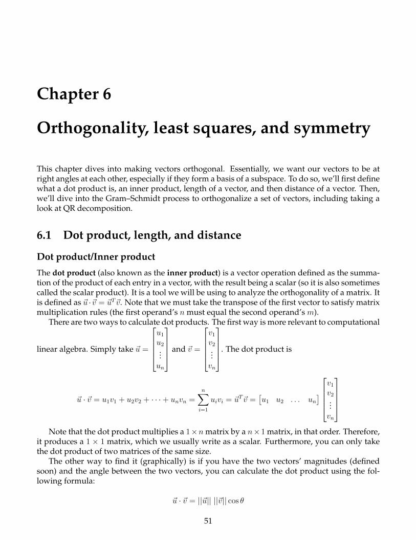
Chapter 6
Orthogonality, least squares, and symmetry
This chapter dives into making vectors orthogonal. Essentially, we want our vectors to be atright angles at each other, especially if they form a basis of a subspace. To do so, we’ll first definewhat a dot product is, an inner product, length of a vector, and then distance of a vector. Then,we’ll dive into the Gram–Schmidt process to orthogonalize a set of vectors, including taking alook at QR decomposition.
6.1 Dot product, length, and distance
Dot product/Inner product
The dot product (also known as the inner product) is a vector operation defined as the summa-tion of the product of each entry in a vector, with the result being a scalar (so it is also sometimescalled the scalar product). It is a tool we will be using to analyze the orthogonality of a matrix. Itis defined as ~u ·~v = ~uT~v. Note that we must take the transpose of the first vector to satisfy matrixmultiplication rules (the first operand’s n must equal the second operand’s m).
There are two ways to calculate dot products. The first way is more relevant to computational
linear algebra. Simply take ~u =
u1u2...un
and ~v =
v1v2...vn
. The dot product is
~u · ~v = u1v1 + u2v2 + · · ·+ unvn =n∑
i=1
uivi = ~uT~v =[u1 u2 . . . un
]v1v2...vn
Note that the dot product multiplies a 1×n matrix by a n×1 matrix, in that order. Therefore,
it produces a 1 × 1 matrix, which we usually write as a scalar. Furthermore, you can only takethe dot product of two matrices of the same size.
The other way to find it (graphically) is if you have the two vectors’ magnitudes (definedsoon) and the angle between the two vectors, you can calculate the dot product using the fol-lowing formula:
~u · ~v = ||~u|| ||~v|| cos θ
51
52 CHAPTER 6. ORTHOGONALITY, LEAST SQUARES, AND SYMMETRY
If the dot product of two vectors equals 0, that means θ = 90◦ and therefore cos(90◦) = 0, sothe dot product will be 0. This also works with component form.
The subspace formed by the dot product is called the inner product space.The dot product has important geometric ramifications. We use the dot product to determine
the length of a vector and the distance between two vectors. More importantly, however, whenthe dot product of two vectors is zero, then we can conclude they are perpendicular, or orthogonalto each other.
This study guide recommends you watch the Essence of Linear Algebra video series for certaintopics in linear algebra in order to get the utmost understanding. Below is the recommendedvideo for this section:
Essence of Linear Algebra – Chapter 7: Dot product and duality:https://www.youtube.com/watch?v=LyGKycYT2v0
Length/magnitude of a vector
When we plot a vector, the length (or magnitude) from its head to its tail is defined by
||~u|| =√~u · ~u =
√(u1)2 + (u2)2 + . . . (un)2
Notice the similarities of this formula to the distance formula you learned in algebra. How-ever, this is not the same as the distance between two vectors, which will be defined next.
The length/magnitude will always be nonnegative and will only be zero when ~u = ~0. Fur-thermore, the following stipulations arise:
• ||~u||2 =√~u · ~u2 = ~u · ~u • ||c~u|| =
√c~u · c~u =
√c2~u · ~u =√
c2√~u · ~u = |c|||~u||
Unit vector
A unit vector is a vector with length 1. The expression
1
||~u||~u
gives us the unit vector in the same direction as ~u.
Distance between two vectors
In the one-dimensional real space R, the distance between two scalars a, b is the absolute valueof their difference, |a− b|. The distance between two vectors in Rn is defined to be
dist(~u,~v) = ||~u− ~v||
6.2 Introduction to orthogonality
This section lays the groundwork for making use of orthogonality-related concepts.
6.2. INTRODUCTION TO ORTHOGONALITY 53
Orthogonal vectors
By definition, two vectors ~u and ~v are orthogonal to each other if their inner product is equal to0. However, any of these three equations would indicate that ~u is orthogonal to ~v.
~u · ~v = 0dist(~u,~v) = dist(~u,−~v)||~u+ ~v||2 = ||~u||2 + ||~v||2
=⇒ ~u ⊥ ~v
Orthogonal complements
If we have a trimmed version of the standard basis Exy =
100
,010
, then we have a 2D plane
(let’s call it the vector space W ). But how would we expand this to all of R3? We simply add avector to this basis with a nonzero value in the third entry. But let’s say we want all of our basisvectors to be orthogonal to each other, because it’s neater that way. And let’s say we only want
unit vectors in our bases. Then there is only one choice: ~e3 =
001
. This vector part of a set of
vectors that are also orthogonal to W (the 2D plane), called an orthogonal complement of W .If a vector ~x is orthogonal to every vector in the subspace W ⊆ Rn, then ~x is orthogonal to
the entire subspace W . The set of all vectors ~x that are orthogonal to W is called the orthogonalcomplement of W , denoted W⊥ (pronounced W perp). W⊥ is a subspace of Rn.
Interestingly enough, the row space’s orthogonal complement is actually the null space. (Notthe column space, because remember the row space and null space are both subspaces of Rn,while the column space is a subspace of Rm). Furthermore, the column space’s orthogonal com-plement is actually just the transpose of the null space.
(RowA)⊥ = NulA and (ColA)⊥ = NulAT
This means that if we have any vector ~u in Rn, ~w ∈ W , and ~v ∈ W⊥, then we can write ~u as asum of ~w and ~v: ~u = ~w + ~v.
Orthogonal sets
An orthogonal set is simply a set of vectors that are all orthogonal to each other. To be specific, aset of vectors {~v1, ~v2, . . . , ~vn} constitutes an orthogonal set if for any two vectors in the set ~vi and~vj their dot product is zero (~vi · ~vj = 0).
The simplest example of an orthogonal set is the standard basis E3 =
100
,010
,001
(in
this case in R3). It’s evident from our above definition that these basis vectors are all orthogonalto each other.
Now, it turns out that the above orthogonal set being a basis is no coincidence. That’s becauseall orthogonal sets are linearly independent and forms a basis for the subspace the orthogonalset spans.
54 CHAPTER 6. ORTHOGONALITY, LEAST SQUARES, AND SYMMETRY
In addition, we can actually backtrack and find each weight of a certain linear combinationof an orthogonal set. If we have an orthogonal basis S = {~u1, ~u2, . . . , ~un} that lives in the sub-space W , then for each vector in the subspace W (which we’ll call ~y), the weights of the linearcombination are given by:
cj =~y · ~uj~uj · ~uj
What we’re essentially doing is compressing the vector ~y onto the same direction as the basisvector ~uj and extracting the scalar multiple cj that is required to equate that component of ~y to~uj .
This has extremely important ramifications. In the next next section, we’ll discuss the projec-tion operator.
Orthonormal sets
If the orthogonal set is comprised of unit vectors, this is called an orthonormal set, and a or-thonormal matrix is a square invertible matrix with orthonormal columns.
An m × n matrix U is orthonormal if and only if UTU = In. Furthermore, for an n × nsquare matrix S that is an orthonormal matrix, we know that S−1S = In, but because it is alsoorthonormal, STS = In is also true. Therefore, for orthonormal matrices (which are square bydefinition), S−1 = ST . We will use these properties later.
Properties of orthonormal sets:
• ||U~x|| = ||~x||
• (U~x) · (U~y) = ~x · ~y
• (U~x) · (U~y) = 0 ⇐⇒ ~x · ~y = 0
Orthogonal projections onto lines
Imagine you have vector ~b flat on the x-axis and ~a pointing up at an angle of 60◦ from ~b. Thenthe ”shadow” that ~a casts upon the direction of~b is called the orthogonal projection (we usuallyjust call it a projection, though).
The projection is found by the following formula:
proj ~b ~a =
(~a ·~b~b ·~b
)~b
~a·~b~b·~b
determines the magnitude, whereas the exact direction of the projection is kept from~b.However, in linear algebra, saying that the projection is simply ”in the direction of ~b” won’t
cut it. So we have to use an even more specific definition. Instead, we define projections tobe onto subspaces and we’ll say that the projection is along the subspace that spans ~b. (In thissubsection, we will stick with a one-dimensional subspace, but in the next section we will explainorthogonal projections onto n-dimensional subspaces in Rn.)
Let’s redefine. Given that L = Span{~b}, an orthogonal projection is given by:
proj L ~a =
(~a ·~b~b ·~b
)~b
Side note: In physics, you can also find parallel and normal forces by using projections.
6.3. ORTHOGONAL PROJECTIONS ONTO SUBSPACES 55
6.3 Orthogonal projections onto subspaces
Earlier, we established that if you have any vector ~u in Rn, ~w ∈ W , and ~v ∈ W⊥, then we canwrite ~u as a sum of ~w and ~v: ~u = ~w + ~v. The projection of ~u onto the subspace W is really just ~w.The same thing applies to the projection of ~u onto W⊥: it’s ~v.
proj W ~u = ~w and proj W⊥ ~u = ~v
The projection operator is basically extracting the ~w component of the vector ~u.From this, we get the Orthogonal Decomposition Theorem: let W ⊆ Rn be a subspace.
Then, you can write any vector ~u in the unique form
~u = ~w + ~v
where ~w ∈ W and ~v ∈ W⊥. ~w is then the orthogonal projection of ~u onto W as we statedabove.
In fact, if {~b1,~b2, . . . ,~bp} is any orthogonal basis of W , then you can write ~u in terms of thisbasis’s projection onto W as the sum of the projections of ~w onto~bi:
~w =~u ·~b1~b1 ·~b1
~b1 + · · ·+~u ·~bp~bp ·~bp
~bp = proj Span{~b1} ~u+ · · ·+ proj Span{~bp} ~u
For a linear transformation, you can use the following formula:
proj W ~u = A(ATA)−1AT~x
6.4 Gram–Schmidt process
The Gram–Schmidt process is a simple algorithm to orthogonalize any basis for any nonzerosubspace in Rn.
If we have any basis {~x1, ~x2, . . . , ~xp} for a nonzero subspace W of Rn, then {~v1, ~v2, . . . , ~vp} isan orthogonal basis for W , where they are defined as follows:
~v1 = ~x1~v2 = ~x2 − proj ~x2
~v1~v3 = ~x3 − proj ~x3
~v1 − proj ~x3~v2
...~vp = ~xp − proj ~xp
~v1 − proj ~xp~v2 − · · · − proj ~xp
~vp−1
This also means that Span{~v1, ~v2, . . . , ~vk} = Span{~x1, ~x2, . . . , ~xk} for 1 ≤ k ≤ p. (In otherwords, Span{~v1} = Span{~x1}, as well as Span{~v1, ~v2} = Span{~x1, ~x2}, etc.)
(In this definition, we use the “primitive” definition of projections, defined as proj ~b ~a = ~a·~b~b·~b~b)
To obtain an orthonormal basis from Gram–Schmidt, simply apply the unit vector formula toeach basis vector in order to orthonormalize (as opposed to simply orthogonalizing) the basis.
56 CHAPTER 6. ORTHOGONALITY, LEAST SQUARES, AND SYMMETRY
QR decomposition
A = QR
QR decomposition is basically converting a matrix A into the equivalent matrix product QRusing the Gram–Schmidt process, where Q is an orthonormal matrix (a matrix whose columnsare an orthonormal basis) for ColA and R is an upper triangular invertible matrix with positiveentries on the diagonal.
Since Q is orthonormal, you can find R by applying the property that QTQ = In (see “Or-thonormal sets” for a refresher), and so A = QR =⇒ QTA = QTQR = R. Therefore, todetermine R, simply do:
R = QTA
6.5 Symmetric matrices
A symmetric matrix is one that is the same when flipped across its diagonal. In other words, if amatrix A = AT , then A is symmetric.
For a diagonalized matrix A = PDP−1, we can say that if P is comprised of an orthonormalbasis, then P−1 can be replaced with P T for computational ease.
A = PDP T ⇐⇒ P is an orthogonal matrix
• If A is symmetric, then any two eigenvectors from different eigenspaces are orthogonal.
• An n× n matrix A is orthogonally diagonalizable if and only if A is a symmetric matrix.
The Spectral Theorem
Remember the spectrum is the set of all the eigenvalues of a matrix A. An n × n symmetricmatrix A has the following properties: (Lay)
• A has n real eigenvalues, including mul-tiplicities.
• The dimension of λ’s eigenspace is equalto its multiplicity in the characteristic
equation.
• The eigenspaces are orthogonal to eachother (mutually orthogonal).
• A is orthogonally diagonalizable.
Spectral decomposition
We can write A = PDP T as A = λ1~u1~uT1 + · · · + λn~un~u
Tn . This is called the spectral decomposi-
tion of A. Every matrix ~ui~uTi is a projection matrix because the vector (~ui~uTi )~x is the orthogonalprojection of ~x onto the subspace spanned by ~ui. (Lay)
Chapter 7
Miscellaneous topics
7.1 Cross products
Cross products are the other way to multiply vectors. They are denoted as ~u × ~v and resultsin a vector perpendicular to both ~u and ~v, which is why they are also sometimes called vectorproducts.
The magnitude of a cross product is found by taking the area of the parallelogram whosesides are formed by the vectors.
For two vectors in R2, simply create a 2 × 2 matrix whose first column is ~u and the secondcolumn is ~v. This matrix represents the linear transformation from the standard basis E to anarbitrary basis B comprised of ~u and ~v. In essence, this matrix is the change-of-coordinatesmatrix from E to B, or P
B←E. Note that the area of the parallelogram whose sides are formed by
the standard basis vectors ~e1 and ~e2 is 1. So the scaled area of this transformed parallelogram isgreater than 1.
For two vectors in R3, you can use the following procedure to find the cross product usingcomponents of the vector. Assuming you are working with the standard basis E , you take thedeterminant of a matrix with the top row as ı̂, ̂, k̂. The result is then a vector. We can alsomake the first column the standard basis vectors and then the next two columns as ~u and ~v, sincedetA = detAT .
~u× ~v =
∣∣∣∣∣∣ı̂ ̂ k̂u1 u2 u3v1 v2 v3
∣∣∣∣∣∣ =∣∣∣∣∣∣ı̂ u1 v1̂ u2 v2k̂ u3 v3
∣∣∣∣∣∣Note that the cross products results in a vector. The determinant gives you a scalar output,
which is the magnitude of the cross product vector. However, its direction is unclear unless youuse the right-hand rule.
Here’s how you use the right-hand rule for ~u × ~v. Start at the first operand (~u) with yourfingers pointed straight. Then curl your fingers towards the second operand (~v). If your thumbpoints upwards, then the result of the cross product is also upwards. Similarly, if your thumbpoints downwards, the result is also downwards. This only works for 2D vectors being crossedthough. For 3D vectors, you must use the determinant method.
If you have the magnitudes of your two vectors and the angle between them, you can simplyuse the following formula:
57
58 CHAPTER 7. MISCELLANEOUS TOPICS
|~u× ~v| = ||~u||||~v|| sin θ
Cross products are anticommunicative, meaning that ~u× ~v = −~v × ~u. In other words, ordermatters!!
There are different ways to calculate the determinant, so if you do not know how to calculateit, please research it.
Additionally, in R2, the magnitude of a cross product is equivalent to the area of the paral-lelogram made if the two operand vectors were placed tail-to-tail and formed a parallelogram.For R3, the magnitude of a cross product would be equivalent to a parallelepiped, which is the 3Dversion of a parallelogram.
This study guide recommends you watch the Essence of Linear Algebra video series for certaintopics in linear algebra in order to get the utmost understanding. Below is the recommendedvideo for this section:
Essence of Linear Algebra – Chapter 8: Cross products:https://www.youtube.com/watch?v=eu6i7WJeinw
Reference material
Full Invertible Matrix Theorem
Let A be an n×n square matrix. If any of the following statements pertaining to A are true, thenthe rest of the statements must also be true.
1. A is an invertible matrix.
2. A is row equivalent to In, the n × n iden-tity matrix.
3. A has n pivot positions. (i.e. there is apivot in every row and every column).
4. The homogeneous matrix equation A~x =~0 has only the trivial solution.
5. The columns of A form a linearly inde-pendent set.
6. The linear transformation x 7→ Ax is one-to-one.
7. The equation A~x = ~b has exactly one so-lution ∀~b ∈ Rn. (∀means ”for all”.)
8. The columns of A span Rn.
9. The linear transformation x 7→ Ax mapsRn onto Rn.
10. There is an n×nmatrixC so thatCA = In.
11. There is an n × n matrix D so that AD =In. C = D always.
12. AT is an invertible matrix.
13. The columns of A form a basis for Rn.
14. ColA = Rn.
15. rankA = n.
16. NulA = {~0}.
17. nullity = 0.
18. RowA = Rn.
19. The number 0 is NOT an eigenvalue of A.(0 /∈ λ)
20. The determinant of A is NOT zero.(detA 6= 0)
21. The orthogonal complement of the col-umn space is {~0}.
22. The orthogonal complement of the nullspace is Rn.
23. The matrix A has n nonzero singular val-ues.
59