arX

iv:h

ep-p

h/02

1216

9v2

5 F

eb 2

003

MC-TH-2002-12SINP/TNP/02-36

WUE-ITP-2002-037hep-ph/0212169December 2002

Neutrinoless Double Beta Decay

from Singlet Neutrinos in Extra Dimensions

G. Bhattacharyya a, H.V. Klapdor-Kleingrothaus b, H. Pas c, A. Pilaftsis d

aSaha Institute of Nuclear Physics, 1/AF Bidhan Nagar, Kolkata 700064, India

bMax-Planck-Institut fur Kernphysik, P.O. Box 103980, D-69029 Heidelberg, Germany

cInstitut fur Theoretische Physik und Astrophysik, Universitat Wurzburg,

Am Hubland, 97074 Wurzburg, Germany

dDepartment of Physics and Astronomy, University of Manchester,

Manchester M13 9PL, United Kingdom

ABSTRACT

We study the model-building conditions under which a sizeable 0νββ-decay signal to the recently

reported level of 0.4 eV is due to Kaluza–Klein singlet neutrinos in theories with large extra dimensions.

Our analysis is based on 5-dimensional singlet-neutrino models compactified on an S1/Z2 orbifold,

where the Standard–Model fields are localized on a 3-brane. We show that a successful interpretation of

a positive signal within the above minimal 5-dimensional framework would require a non-vanishing shift

of the 3-brane from the orbifold fixed points by an amount smaller than the typical scale (100 MeV)−1

characterizing the Fermi nuclear momentum. The resulting 5-dimensional models predict a sizeable

effective Majorana-neutrino mass that could be several orders of magnitude larger than the light

neutrino masses. Most interestingly, the brane-shifted models with only one bulk sterile neutrino also

predict novel trigonometric textures leading to mass scenarios with hierarchical active neutrinos and

large νµ-ντ and νe-νµ mixings that can fully explain the current atmospheric and solar neutrino data.

1

1 Introduction

Recently, realizations of phenomenologically viable theories with large compact dimensions

of TeV size [1] have enriched dramatically our perspectives in searching for physics beyond the

Standard Model (SM). Among the possible higher-dimensional realizations, sterile neutrinos

propagating in large extra dimensions [2, 3, 4, 5, 6, 7, 8, 9] may provide interesting alternatives

for generating the observed light neutrino masses. On the other hand, detailed experimental

studies of neutrino properties may even shed light on the geometry and/or shape of the new

dimensions. In this context, one of the most sensitive experimental approaches to neutrino

masses and their properties is the search for neutrinoless double beta decay [10]. Neutrinoless

double beta decay, denoted in short as 0νββ, corresponds to two single beta decays [11, 12]

occurring simultaneously in one nucleus, thereby converting a nucleus (Z,A) into a nucleus

(Z + 2, A), i.e.AZ X → A

Z+2X + 2e− .

This process violates lepton number by two units and hence its observation would signal physics

beyond the SM. To a very good approximation, the half life for a 0νββ decay mediated by light

neutrinos is given by

[T 0νββ1/2 ]−1 =

|〈m〉|2m2

e

|M0νββ|2G01 , (1.1)

where 〈m〉 denotes the effective neutrino Majorana mass, me is the electron mass and M0νββ

and G01 denote the appropriate nuclear matrix element and the phase space factor, respectively.

For details, see [10, 11, 12] and our discussion in Section 4.

Most recently, the Heidelberg–Moscow collaboration has reanalyzed its experimental

data [13], using appropriate statistical methods as well as new information from the form

of the contributing background. They found an excess of 0νββ events, with statistical signifi-

cance 2.2–3.1 σ depending on the method used. From this result, a half-life of 1.5+16.8−0.7 × 1025

years at 95% confidence level (CL) for 76Ge is deduced, which implies an absolute value for the

effective Majorana-neutrino mass:

|〈m〉| = 0.39+0.45−0.34 eV (95% CL) , (1.2)

allowing an uncertainty of the nuclear matrix element values of ±50%.

The above experimental result (1.2), combined with information from solar and atmo-

spheric neutrino data, restricts the admissible forms of the light-neutrino mass hierarchies

in 4-dimensional models with 3 left-handed (active) neutrinos. The allowed scenarios contain

either degenerate neutrinos or neutrinos that have an inverse mass hierarchy [14]. Evidently,

2

a successful interpretation of a positive 0νββ signal of the appropriate size mentioned above

imposes certain constraints on the structure of a theory. Here, we study these constraints on

the model building of minimal 5-dimensional theories compactified on a S1/Z2 orbifold. Within

the framework of theories with large extra dimensions, previous studies on neutrinoless double

beta decays were performed within the context of higher-dimensional models that utilize the

shining mechanism from a distant brane [15] and of theories with wrapped geometric space [16].

In Ref. [15], the 0νββ decay is accompanied with emission of Majorons, whereas the prediction

in [16] falls short by two orders of magnitude to account for the observable excess in (1.2).

In this paper, we consider an even more minimal higher-dimensional framework of lepton-

number violation, in which only one 5-dimensional (bulk) sterile neutrino is added to the field

content of the SM. In this minimal model, the SM fields are localized on a 4-dimensional

Minkowski subspace, also termed 3-brane. The violation of the lepton number may oc-

cur in three distinct ways: (i) by adding lepton-number violating bilinears of the Majorana

type in the Lagrangian; (ii) by generating lepton-number-violating mass terms through the

Scherk–Schwartz mechanism [17]; (iii) by simultaneously coupling the Z2-even and Z2-odd two-

component spinors of the 5-dimensional sterile neutrino to the same left-handed charged lepton

state. As we will see in Section 2, the last case (iii) is only possible if the 3-brane describing our

observable world is shifted from the S1/Z2 orbifold fixed point. Here, we should also note that

after integration of the extra dimension, the 5-dimensional orbifold model predicts an infinite

tower of Kaluza–Klein (KK) neutrinos, for which the cases (i) and (ii) become fully equivalent.

One salient feature of the S1/Z2 orbifold compactification is that the KK neutrinos group

themselves into approximately degenerate pairs of opposite CP parities. As a result, the lepton-

number-violating KK-neutrino effects cancel each other and so the predicted 0νββ decay turns

out to be exceedingly small to account for the recent observable excess. The latter appears to

be a major obstacle in theories with large extra dimensions and imposes by itself constraints

on the model-building of higher-dimensional theories. A minimal way that avoids the above

disastrous CP-parity cancellation effects on the 0νββ decay amplitude would be to arrange

the opposite CP-parity KK neutrinos to couple to the W± bosons with unequal strength.

Within the minimal 5-dimensional orbifold model outlined above, such a realization can be

accomplished only if the 3-brane is displaced from one of the S1/Z2 orbifold fixed points. In

our phenomenological bottom-up approach, the amount of brane-shifting is not arbitrary but

dictated by the requirement that the model can accommodate the result (1.2) for the effective

Majorana-neutrino mass. In particular, we will see in Section 4 how the resulting brane-shifted

5-dimensional models can predict a sizeable effective Majorana-neutrino mass that could be

several orders of magnitude larger than the light neutrino masses and hence than the difference

of their squares as required from neutrino oscillation data.

3

Another important constraint on the structure of higher-dimensional neutrino theories arises

from their ability to explain the solar and atmospheric neutrino data by means of neutrino

oscillations. In particular, orbifold models with one bulk neutrino, as those considered earlier

in the literature [2, 4, 7, 8, 9], seem to prefer the Small Mixing Angle (SMA) Mikheev-Smirnov-

Wolfenstein (MSW) solution [18] which is highly disfavoured by recent neutrino data analyses.

Alternatively, if all neutrino data are to be explained by oscillations of active neutrinos with

a small admixture of sterile KK component, then the compactification scale has to be much

higher than the brane-Dirac mass terms. After integrating out the bulk neutrino of the model,

the effective light-neutrino mass matrix has a rather restricted form; it is effectively of rank 1.

As a result, two out of the three active neutrinos are massless. This is rather undesirable, since

only one neutrino-mass difference can be formed in this case, so accommodating all neutrino

oscillation data proves rather problematic [7,8,9]. However, the earlier studies have not included

the possibility of a shifted brane. As was mentioned above, brane-shifting gives rise to sizeable

lepton-number violation. Hence, the tree-level rank-1 form of the effective neutrino mass matrix

can be significantly modified through lepton-number violating Yukawa terms. As we will see in

Section 5, the resulting neutrino mass matrix has sufficiently rich structure to enable adequate

description of the neutrino data.

Our paper is organized as follows: Section 2 describes the low-energy structure of the 5-

dimensional orbifold models. Technical details are relegated to the appendices. In Section 3,

we study the renormalization-group (RG) effects of the neutrino Yukawa couplings and their

possible impact on the 0νββ decay amplitude. In Section 4 we give estimates of the effective

Majorana-neutrino mass, which are predicted in these models presented in Section 2. In Section

5, we discuss the compatibility of such models with solar and atmospheric neutrino data.

Finally, we draw our conclusions in Section 6.

2 Minimal higher-dimensional neutrino models

In this section, we will describe the basic low-energy structure of minimal higher-dimensional

extensions of the SM that include singlet neutrinos. In particular, we assume that singlet

neutrinos being neutral under the SU(2)L⊗U(1)Y gauge group can freely propagate in a higher-

dimensional space of [1 + (3 + δ)] dimensions, the so-called bulk, whereas all SM particles are

localized in a (1 + 3)-dimensional subspace, known as 3-brane or simply brane. However, even

singlet neutrinos themselves may live in a subspace of an even higher-dimensional space of

[1 + (3 + ng)] dimensions, with δ ≤ ng, in which gravity propagates.

4

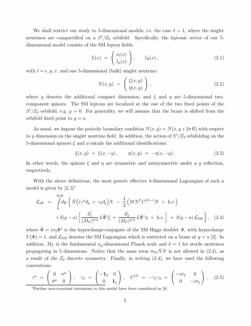
We shall restrict our study to 5-dimensional models, i.e. the case δ = 1, where the singlet

neutrinos are compactified on a S1/Z2 orbifold. Specifically, the leptonic sector of our 5-

dimensional model consists of the SM lepton fields:

L(x) =

νl(x)

lL(x)

, lR(x) , (2.1)

with l = e, µ, τ , and one 5-dimensional (bulk) singlet neutrino:

N(x, y) =

ξ(x, y)

η(x, y)

, (2.2)

where y denotes the additional compact dimension, and ξ and η are 5-dimensional two-

component spinors. The SM leptons are localized at the one of the two fixed points of the

S1/Z2 orbifold, e.g. y = 0. For generality, we will assume that the brane is shifted from the

orbifold fixed point to y = a.

As usual, we impose the periodic boundary condition N(x, y) = N(x, y+2πR) with respect

to y dimension on the singlet neutrino field. In addition, the action of S1/Z2 orbifolding on the

5-dimensional spinors ξ and η entails the additional identifications:

ξ(x, y) = ξ(x,−y) , η(x, y) = −η(x,−y) . (2.3)

In other words, the spinors ξ and η are symmetric and antisymmetric under a y reflection,

respectively.

With the above definitions, the most generic effective 4-dimensional Lagrangian of such a

model is given by [2, 5]1

Leff =

2πR∫

0

dy{

N(

iγµ∂µ + γ5∂y)

N − 1

2

(

MNTC(5)−1N + h.c.)

+ δ(y − a)[

hl1

(MF )δ/2LΦ∗ξ +

hl2

(MF )δ/2LΦ∗η + h.c.

]

+ δ(y − a)LSM

}

, (2.4)

where Φ = iσ2Φ∗ is the hypercharge-conjugate of the SM Higgs doublet Φ, with hypercharge

Y (Φ) = 1, and LSM denotes the SM Lagrangian which is restricted on a brane at y = a [2]. In

addition, MF is the fundamental ng-dimensional Planck scale and δ = 1 for sterile neutrinos

propagating in 5 dimensions. Notice that the mass term mDNN is not allowed in (2.4), as

a result of the Z2 discrete symmetry. Finally, in writing (2.4), we have used the following

conventions:

γµ =

0 σµ

σµ 0

, γ5 =

−12 0

0 12

, C(5) = −γ1γ3 =

−iσ2 0

0 −iσ2

, (2.5)

1Further non-covariant extensions to this model have been considered in [8].

5

with σµ = (12,σ) and σµ = (12,−σ), where σ1,2,3 are the usual Pauli matrices.

We now proceed with the compactification of the y dimension of the S1/Z2 orbifold model.

Because of their symmetric and antisymmetric properties (2.3) under y reflection, the two-

component spinors ξ and η can be expanded in a Fourier series of cosine and sine harmonics:

ξ(x, y) =1√2πR

ξ0(x) +1√πR

∞∑

n=1

ξn(x) cos(

ny

R

)

, (2.6)

η(x, y) =1√πR

∞∑

n=1

ηn(x) sin(

ny

R

)

, (2.7)

where the chiral spinors ξn(x) and ηn(x) form an infinite tower of KK modes.

After substituting (2.6) into (2.4) and integrating out the y coordinate, we obtain the

effective 4-dimensional Lagrangian

Leff = LSM + ξ0(iσµ∂µ)ξ0 +

(

hl(0)1 LΦ∗ξ0 − 1

2M ξ0ξ0 + h.c.

)

+∞∑

n=1

[

ξn(iσµ∂µ)ξn

+ ηn(iσµ∂µ)ηn +

n

R

(

ξnηn + ξnηn)

− 1

2M(

ξnξn + ηnηn + h.c.)

+√2(

hl(n)1 LΦ∗ξn + h

l(n)2 LΦ∗ηn + h.c.

)

]

, (2.8)

where

hl(n)1 =

hl1

(2πMFR)δ/2cos

(

na

R

)

=(

MF

MP

)δ/ng

hl1 cos

(

na

R

)

, (2.9)

hl(n)2 =

hl2

(2πMFR)δ/2sin

(

na

R

)

=(

MF

MP

)δ/ng

hl2 sin

(

na

R

)

. (2.10)

In deriving the last step on the RHS’s of (2.9) and (2.10), we have employed the basic rela-

tion among the Planck mass MP, the corresponding ng-dimensional Planck mass MF and the

compactification radii R (all taken to be of equal size):

MP = (2πMF R)ng/2 MF . (2.11)

From (2.9) and (2.10), we see that the reduced 4-dimensional Yukawa couplings h(n)1,2 can be

suppressed by many orders of magnitude [3, 2] if there is a large hierarchy between MP and

the quantum gravity scale MF . Thus, if gravity and bulk neutrinos feel the same number of

extra dimensions, i.e. δ = ng, the 4-dimensional Yukawa couplings h(n)1 and h

(n)2 are naturally

suppressed by a huge factor MF/MP ∼ 10−15, for MF ≈ 10 TeV. From (2.2), we observe that

ξ and η belong to the same multiplet and hence have the same lepton number. It then follows

from (2.8) that the simultaneous presence of h(n)1 and h

(n)2 in an amplitude gives rise to lepton

number violation by two units.

6

We should note that the above large suppression factor can be also obtained in a 5-

dimensional neutrino model (δ = 1), where gravity propagates in a 6-dimensional space with

compactification radii R1 and R2 of unequal size (ng = 2). In this case, one has to use the

general toroidal compactification condition:

MP = (2πMF )ng/2 (R1R2 . . . Rng

)1/2MF . (2.12)

Note that (2.12) reduces to (2.11) if all compactification radii are equal. With the help of

(2.12), we find for ng = 2

hl1,2

(2πMFR1)1/2= (2πMFR2)

1/2 MF

MP

hl1,2 . (2.13)

We easily see that if R2 ∼ 1/MF , the original Yukawa couplings hl1,2 undergo the same large

degree of suppression by a factor MF/MP.

If the brane were located at the one of the two orbifold fixed points, e.g. at y = 0, the

operator LΦ∗η would be absent as a consequence of the Z2 discrete symmetry. However, if the

brane is shifted by an amount a 6= 0, the above operator is no longer absent. In fact, as we

will see in Section 4, the coexistence of the two operators LΦ∗ξ and LΦ∗η breaks the lepton

number leading to observable effects in neutrinoless double beta decay experiments.

Let us now introduce the weak basis for the KK-Weyl spinors

χ±n =1√2( ξn ± ηn ) , (2.14)

which enables to express the effective kinetic term of the neutrino sector as follows:

Lkin = χ iσµ∂µ χ −(

1

2χT Mχ + h.c.

)

, (2.15)

where χT = (νl, ξ0, χ1, χ−1, . . . , χn, χ−n, . . . ) and

MKK =

0 m m m m m · · ·m M 0 0 0 0 · · ·m 0 M + 1

R0 0 0 · · ·

m 0 0 M − 1R

0 0 · · ·m 0 0 0 M + 2

R0 · · ·

m 0 0 0 0 M − 2R

· · ·...

......

......

.... . .

, (2.16)

with m = vh1/√2. In a three-generation model, m and h1 are both 3-vectors in the flavour

space, i.e. h1 = (he1, hµ

1 , hτ1)

T . We will discuss intergenerational mixing effects in more detail

in Section 5. Here, we assume for simplicity that h1 = he1.

7

Following [2], we rearrange the singlet KK-Weyl spinors ξ0 and χ±n , such that the smallest

diagonal entry of the KK neutrino mass matrixMKK in (2.16) is |ε| = min(

|M− kR|)

≤ 1/(2R),

for a given value k = k0. In this newly defined basis, the effective kinetic Lagrangian (2.15)

becomes

Lkin =1

2Ψν

(

i 6∂ − MKKν

)

Ψν , (2.17)

where Ψν is the reordered (4-component) Majorana-spinor vector

ΨTν =

νl

νl

,

χk0

χk0

,

χk0+1

χk0+1

,

χk0−1

χk0−1

, · · · ,

χk0+n

χk0+n

,

χk0−n

χk0−n

, · · ·

(2.18)

and MKKν the corresponding KK neutrino mass matrix

MKKν =

0 m m m m m · · ·m ε 0 0 0 0 · · ·m 0 ε+ 1

R0 0 0 · · ·

m 0 0 ε− 1R

0 0 · · ·m 0 0 0 ε+ 2

R0 · · ·

m 0 0 0 0 ε− 2R

· · ·...

......

......

.... . .

. (2.19)

The eigenvalues of MKKν can be computed from the characteristic eigenvalue equation

det (MKKν − λ1) = 0, which is analytically given by

∞∏

n=0

[

(

λ − ε)2 − n2

R2

] [

1 +ε

λ − ε− m2

∞∑

n=−∞

1

(λ − ε)2 − n2

R2

]

= 0 . (2.20)

Since it can be shown that λ − ε = ±n/R is never an exact solution to the characteristic

equation, only the second factor in (2.20) can vanish. Employing complex contour integration

techniques, the summation in the second factor in (2.20) can be performed exactly, leading to

an equivalent transcendental equation

λ = πm2R cot[

πR (λ− ε)]

. (2.21)

As was already discussed in [2], if ε = 0, (2.21) implies that the mass spectrum consists of

massive KK Majorana neutrinos degenerate in pairs with opposite CP parities. If ε = 1/(2R),

the KK mass spectrum contains a massless state, which is predominantly left-handed ifmR < 1,

while the remaining massive KK states form degenerate pairs with opposite CP parities, exactly

as in the ε = 0 case. However, if ε 6= 0, 1/(2R), the lepton number gets broken.2 In this case,

2Alternatively, the lepton number may also be broken through the Scherk-Schwarz mechanism, where the

Scherk-Schwarz rotation angle will induce terms very similar to those depending on ε [2, 19].

8

there is no massless state in the spectrum, and the above exact degeneracy among the massive

Majorana neutrinos becomes only approximate, with a mass splitting of order 2ε for each

would-be (ε → 0) degenerate KK pair.

We now consider an orbifold model, in which the y = 0 brane is displaced from the orbifold

fixed points by an amount a. Under certain restrictions in Type I string theory [20, 2], such

an operation can be performed respecting the Z2 invariance of the original higher-dimensional

action. In particular, one can take explicitly account of this last property by considering the

following replacements in the effective Lagrangian (2.4):

ξ δ(y − a) → 1

2ξ[

δ(y − a) + δ(y + a− 2πR)]

,

η δ(y − a) → 1

2η[

δ(y − a) − δ(y + a− 2πR)]

, (2.22)

with 0 ≤ a < πR and 0 ≤ y ≤ 2πR. It is obvious that a Z2-invariant implementation of brane-

shifted couplings requires the existence of two branes at least, placed at y = a and y = 2πR−a.

In addition, we assume that a is a rational number in units of πR, i.e.

a =r

qπR , (2.23)

where r, q are natural numbers. This last assumption has been introduced for technical reasons.

It enables us to carry out analytically the infinite summations over KK states (see also our

discussion below).

Proceeding as above, the effective KK neutrino mass matrix MKKν for the orbifold model

with a shifted brane can be written down in an analogous form

MKKν =

0 m(0) m(1) m(−1) m(2) m(−2) · · ·m(0) ε 0 0 0 0 · · ·m(1) 0 ε+ 1

R0 0 0 · · ·

m(−1) 0 0 ε− 1R

0 0 · · ·m(2) 0 0 0 ε+ 2

R0 · · ·

m(−2) 0 0 0 0 ε− 2R

· · ·...

......

......

.... . .

, (2.24)

where

m(n) =v√2

[

h1 cos(

(n− k0)a

R

)

+ h2 sin(

(n− k0)a

R

) ]

= m cos(

na

R− φh

)

, (2.25)

with m = v√

(h21 + h2

2)/2 and φh = tan−1(h2/h1) + k0a/R. As before, we consider an one-

generation model with h1 = he1 and h2 = he

2, which renders the analytic determination of the

9

eigenvalue equation tractable. We will relax this assumption in Section 5, when discussing

the compatibility of this model with neutrino oscillation data. Thus, for our one-generation

brane-shifted model, the characteristic eigenvalue equation reads

∞∏

n=0

[

(

λ − ε)2 − n2

R2

] [

1 +ε

λ − ε− 1

λ− ε

∞∑

n=−∞

m(n) 2

λ − ε − nR

]

= 0 , (2.26)

which is equivalent to

λ =∞∑

n=−∞

m(n) 2

λ − ε − nR

. (2.27)

As opposed to the a = 0 case, complex contour integration techniques are not directly applicable

in evaluating the infinite sum in (2.27). The preventive reason is that the function m(n),

analytically continued to the complex n-plane, is not bounded from above as n → ±i∞, as it

had to be, because of its dependence on cos(na/R). However, as has been mentioned above and

discussed further in Appendix A, this difficulty may be circumvented by assuming that a is a

rational number in units of πR, as stated in (2.23). Under this technical assumption, we carry

out in Appendix A the infinite sum in (2.27) analytically and derive the eigenvalue equation

for the simplest class of cases, where a = πR/q with r = 1 and q an integer larger than 1, i.e.

q ≥ 2. More precisely, we find 3

λ = πm2R{

cos2[

φh − a(λ− ε)]

cot[

πR (λ− ε)]

− 1

2sin

[

2φh − 2a(λ− ε)]

}

. (2.28)

Observe that unless ε = 1/(2R), a = πR/2 and φh = π/4, the mass spectrum consists of massive

non-degenerate KK neutrinos. However, it can be shown from (2.28) that this tree-level mass

splitting between a pair of KK Majorana neutrinos is generally small for m(n) ≫ 1/R. In

particular, this tree-level mass splitting is almost independent of a and subleading so as to play

any relevant role in our calculations.

At this stage, it is important to comment on taking the limit a = πR/q → 0 in (2.28), or

equivalently q → ∞. This limit is not the eigenvalue equation (2.21) which is valid for a = 0,

because of the presence of the extra non-vanishing term that depends on sin(2φh) in (2.28). This

apparent paradox can be resolved by noticing that the existence of this would-be anomalous

term is ensured only if the brane-shifting a is much larger than the fundamental quantum

gravity scale MF , i.e. a ≫ 1/MF . Since MF represents a natural ultra-violet cut-off of the

theory, we expect the onset of new physics above the scale MF , most likely of stringy nature,

effectively implying that the KK-Yukawa mass terms m(n) are exponentially suppressed or zero

for KK-numbers n >∼ MFR. As we will explicitly demonstrate in Section 4 (see our discussion

3The so-derived formula generalizes the one presented in [2] to include brane-shifting and arbitrary Yukawa-

coupling effects.

10

in (4.18)), such a truncation of the KK sum at MF effectively results in a modification of the

eigenvalue equation (2.28) to

λ = m2R{

π cos2[

φh − a(λ− ε)]

cot[

πR (λ− ε)]

− Si(2aMF ) sin[

2φh − 2a(λ− ε)]

}

. (2.29)

In the above, Si(x) =∫ x0 dt sin t

tis the integral-sine function. For any finite value of its argument,

Si(x) can be expanded as

Si(x) =+∞∑

n=1

(−1)(n−1) x(2n−1)

(2n− 1) (2n− 1)!. (2.30)

For small x, it is Si(x) ≈ x, while Si(x) = π/2 for x → ∞. Clearly, as long as a ≫ 1/MF , the

eigenvalue equations (2.28) and (2.29) are almost identical, since Si(2aMF ) = π/2 to a very

good approximation. On the other hand, the limit a → 0 does now smoothly go over to (2.21),

as it should be.

Finally, in addition to the aforementioned tree-level mass splitting, one-loop radiative effects

may also contribute to further increase the mass difference between two nearly degenerate KK

Majorana neutrinos, if h1 and h2 do not vanish simultaneously. The one-loop generated mass

splitting, however, is expected to be small [5] of order h1h2m(n)/(8π2) ∼ 10−2 × (MF/MP )

2 ×m(n)

<∼ 10−2 ×∆m(n), where m(n) ≈ n/R ≤ MF is the approximate mass of the nth KK pair of

nearly degenerate Majorana neutrinos, and ∆m(n) = m(n+1)−m(n) ≈ 1/R is the mass difference

between two adjacent KK Majorana pairs. Although such a radiatively-induced mass splitting

may play a significant role for leptogenesis [5], its effect on the double beta decay amplitude

is negligible. Therefore, we neglect radiative effects on the KK mass spectrum throughout the

paper.

3 RG evolution of neutrino Yukawa couplings

The RG evolution of the Yukawa couplings in the standard 4-dimensional scenario involving

sterile neutrinos has been discussed in [21]. Here, we derive the corresponding RG equations

for the higher-dimensional case. Since the RG evolution equations for hl1 and hl

2 will be similar,

we concentrate only on the former (≡ h). In such a higher-dimensional scenario, the presence

of the KK sterile states alters the RG running. The triangle and self-energy diagrams that

contribute to the running remain the same as in the SM, except that in the higher dimensional

context, wherever there are internal ξn lines, there is a multiplicative factor tδ = (µR)δXδ, with

11

Xδ = 2πδ/2/δΓ(δ/2). The RG equation for the Yukawa coupling h is given by

16π2 dh

d lnµ=

3

2

[

tδ (hh†) h− h (h†

ehe)]

+ hTr(

3h†uhu + 3h†

dhd + h†ehe + tδ h

†h)

− h(

9

4g2w +

3

4g′2)

, (3.1)

where gw and g′ are the SU(2)L and U(1)Y gauge-coupling constants, respectively. Note that for

δ = 0 (1), it is Xδ = 1 (2). Also, for δ = 0, tδ = 1, the standard RG equation is reproduced [21].

We now observe that the four-dimensional Yukawa coupling (h) is suppressed with respect

to the higher-dimensional coupling (h) by means of the relation: h = (MF/MP )δ/ngh. Thus,

even if we consider h(1/R) ∼ 1, the four-dimensional h is suppressed by many orders of mag-

nitude. From Eq. (3.1), it is also obvious that unless tδ is large enough to be comparable with

(M2P/M

2F )

δ/ng , the contributions from the top-quark Yukawa coupling or the gauge couplings

dominate the running, and hence there is no power-law behaviour at lower energies.

On the contrary, if we go to a very high energy such that we can ignore ht, then the terms

multiplying tδ dominate. In such a case, ignoring the gauge contribution, we can write

16π2 dh

d lnµ∼ 5

2tδ h

3 . (3.2)

Integrating Eq. (3.2) from the scale µ0 ≡ R−1 to µ, we obtain

1

h2(1/R)− 1

h2(µ)≃ 5Xδ

16π2δ(µR)δ . (3.3)

In terms of the Yukawa fine structure constant α(µ) = h2(µ)/(4π) of the original 5-dimensional

Yukawa coupling (h) and for the simple case δ = ng, (3.3) takes on the form

1

α(µ)≃ 1

α(1/R)− 5Xδ

4πδ

(

µ

MF

)δ

. (3.4)

Clearly, α(µ) → ∞, for a critical scale

µcritical = MF

(

4πδ

5Xδ α(1/R)

)1/δ

(3.5)

Interestingly enough, (3.5) implies that the power-law behaviour sets in not just above the

compactification scale R−1, as was naively expected [2], but well above the quantum gravity

scale MF . On the other hand, requiring that α(MF ) ≤ 1 in (3.4) implies that α(1/R) < 0.55

for δ = 1. This last condition assures that our theory remains perturbative up to the quantum

gravity scale MF . From our discussion above, it is obvious that power-law effects on the Yukawa

neutrino couplings can be safely neglected in our analysis.

12

4 Effective neutrino-mass estimates

In this section, we calculate the 0νββ observable 〈m〉 in orbifold 5-dimensional models. This

quantity determines the size of the neutrinoless double beta decay amplitude, which is induced

by W -boson exchange graphs. To this end, it is important to know the interactions of the W±

bosons to the charged leptons l = e, µ, τ and the KK-neutrino mass-eigenstates n(n). Adopting

the conventions of [22], the effective charged current Lagrangian is given by

LW±

int = − gw√2W−µ

∑

l=e,µ,τ

(

Blνl l γµPL νl ++∞∑

n=−∞

Bl,n l γµPL n(n)

)

+ h.c. , (4.1)

where gw is the weak coupling constant, PL = (1− γ5)/2 is the left-handed chirality projector,

and B is an infinite dimensional mixing matrix. The matrix B satisfies the following crucial

identities:

BlνlB∗l′νl

++∞∑

n=−∞

Bl,nB∗l′,n = δll′ , (4.2)

Blνl mνl Bl′νl ++∞∑

n=−∞

Bl,nm(n) Bl′,n = 0 . (4.3)

Equation (4.2) reflects the unitarity properties of the charged lepton weak space, and (4.3) holds

true, as a result of the absence of the Majorana mass terms νlνl′ from the effective Lagrangian

in the flavour basis. For the models under discussion, the KK neutrino masses m(n) can be

determined exactly by the solutions of the corresponding transcendental equations. To a good

approximation, however, these solutions for large n simplify to4

m(n) ≈ n

R+ ε . (4.4)

This last expression proves to be a good approximation in our estimates.

According to (1.1), the 0νββ-decay amplitude T0νββ is given by [11]:

T0νββ =〈m〉me

MGTF(mν) , (4.5)

where MGTF = MGT −MF is the difference of the nuclear matrix elements for the so-called

Gamow-Teller and Fermi transitions. Note that this difference of nuclear matrix elements

4For |n| > ε and n < 0, the KK mass eigenvalues m(n) are negative. This corresponds to a neutrino with

positive physical mass |m(n)| and negative CP parity. One can always take account of the negative CP parity

by redefining the mixing matrix elements Bl,−n as Bl,−n → iBl,−n, for n > εR > 0. Although we will allow

negative neutrino masses in our calculations, we should stress that both approaches are fully equivalent leading

to the same analytic results.

13

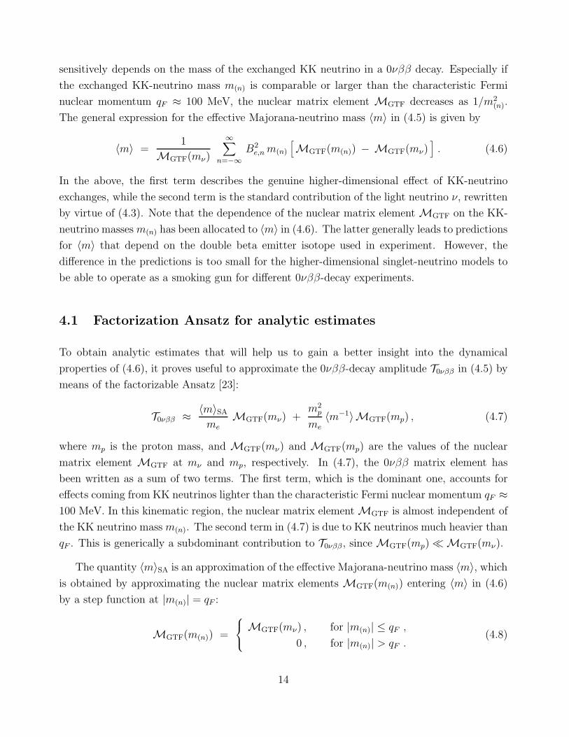
sensitively depends on the mass of the exchanged KK neutrino in a 0νββ decay. Especially if

the exchanged KK-neutrino mass m(n) is comparable or larger than the characteristic Fermi

nuclear momentum qF ≈ 100 MeV, the nuclear matrix element MGTF decreases as 1/m2(n).

The general expression for the effective Majorana-neutrino mass 〈m〉 in (4.5) is given by

〈m〉 =1

MGTF(mν)

∞∑

n=−∞

B2e,nm(n)

[

MGTF(m(n)) − MGTF(mν)]

. (4.6)

In the above, the first term describes the genuine higher-dimensional effect of KK-neutrino

exchanges, while the second term is the standard contribution of the light neutrino ν, rewritten

by virtue of (4.3). Note that the dependence of the nuclear matrix element MGTF on the KK-

neutrino massesm(n) has been allocated to 〈m〉 in (4.6). The latter generally leads to predictions

for 〈m〉 that depend on the double beta emitter isotope used in experiment. However, the

difference in the predictions is too small for the higher-dimensional singlet-neutrino models to

be able to operate as a smoking gun for different 0νββ-decay experiments.

4.1 Factorization Ansatz for analytic estimates

To obtain analytic estimates that will help us to gain a better insight into the dynamical

properties of (4.6), it proves useful to approximate the 0νββ-decay amplitude T0νββ in (4.5) by

means of the factorizable Ansatz [23]:

T0νββ ≈ 〈m〉SAme

MGTF(mν) +m2

p

me〈m−1〉MGTF(mp) , (4.7)

where mp is the proton mass, and MGTF(mν) and MGTF(mp) are the values of the nuclear

matrix element MGTF at mν and mp, respectively. In (4.7), the 0νββ matrix element has

been written as a sum of two terms. The first term, which is the dominant one, accounts for

effects coming from KK neutrinos lighter than the characteristic Fermi nuclear momentum qF ≈100 MeV. In this kinematic region, the nuclear matrix element MGTF is almost independent of

the KK neutrino mass m(n). The second term in (4.7) is due to KK neutrinos much heavier than

qF . This is generically a subdominant contribution to T0νββ , since MGTF(mp) ≪ MGTF(mν).

The quantity 〈m〉SA is an approximation of the effective Majorana-neutrino mass 〈m〉, whichis obtained by approximating the nuclear matrix elements MGTF(m(n)) entering 〈m〉 in (4.6)

by a step function at |m(n)| = qF :

MGTF(m(n)) =

MGTF(mν) , for |m(n)| ≤ qF ,

0 , for |m(n)| > qF .(4.8)

14

In what follows, we refer to such an approach to the nuclear matrix elements as the Step

Approximation (SA). The effective neutrino mass in the SA reads:

〈m〉SA = B2eνmν +

[(qF−ε)R]∑

n=−[(qF+ε)R]

B2e,nm(n)

= −+∞∑

n=[(qF−ε)R]

B2e,nm(n) −

+∞∑

n=[(qF+ε)R]

B2e,−nm(−n) , (4.9)

where we used (4.3) to arrive at the last equality for the effective neutrino mass. Notice that

〈m〉 is not zero, simply because the sum over the KK neutrino states is truncated to those with

a mass |m(n)|, |m(−n)| ≤ qF .

Correspondingly, the effects of the heavier KK neutrinos, with masses m(n)>∼ qF , have been

taken into account in the factorizable Ansatz (4.7) by means of the inverse effective neutrino

mass 〈m−1〉. This newly introduced quantity is given by

〈m−1〉 =+∞∑

n=[(qF−ε)R]

B2e,nm

−1(n) +

+∞∑

n=[(qF+ε)R]

B2e,−nm

−1(−n) . (4.10)

The factorizable form (4.5) of the matrix element constitutes a good approximation except for

the isolated region where |m(n)| ≈ qF ≈ 100 MeV. Nevertheless, the effect of the KK neutrinos

on the effective neutrino mass is cumulative [6] due to a sum of an infinite number of states,

since each KK state has either a tiny Majorana mass or a very suppressed mixing with the

electron neutrinos. Therefore, we expect that excluding this isolated region of KK-neutrino

contributions around qF will not alter quantitatively our results in a relevant way.

We will now rely on (4.9) to estimate the effective neutrino mass 〈m〉SA in different settings

of 5-dimensional orbifold models discussed in Section 2. To begin with, let us consider a simple

orbifold model, with ε 6= 0 and ε 6= 1/(2R). In addition, we consider the case a = 0, namely

we take the brane to be located at the one of the two orbifold fixed points. Like the neutrino

masses, the mixing-matrix elements Beν and Be,n can also be computed exactly [2]:

Beν =1

N , Be,n =1

N(n)

, (4.11)

where the squares of the normalization factors N and N(n) are given by

N 2 = 1 ++∞∑

n=−∞

m2

(

ε − mν + nR

)2 , N 2(n) = 1 +

+∞∑

k=−∞

m2

(

ε − m(n) + kR

)2 . (4.12)

Applying complex integration methods for convergent infinite sums, the squared normalization

factor N 2 can be calculated to give

N 2 = 1 +π2m2R2

sin2[πR(mν − ε)]= 1 + π2m2R2 +

m2ν

m2. (4.13)

15

In obtaining the last equality in (4.13), we used the eigenvalue equation (2.21) for λ = mν .

From (4.11) and (4.13), we immediately see that if mR ≪ 1 and mν ≪ m, it is Beν ≈ 1

and hence the lightest neutrino state is predominantly left-handed. For the calculation of the

effective neutrino mass, we need

N 2(n) = 1 +

π2m2R2

sin2[πR(m(n) − ε)]= 1 + π2m2R2 +

m2(n)

m2≈ ( n

R+ ε )2

m2, (4.14)

where the last approximate equality in (4.14) corresponds to a large n. In Appendix B, we

show that the KK neutrino masses derived from (2.21) and the mixing-matrix elements given

in (4.11) satisfy the sum rules given by the identities (4.2) and (4.3).

Based on (4.9), we will now perform an estimate of the effective neutrino mass in the simple

orbifold model mentioned above. Plugging the value of Be,n = 1/N(n) into (4.9), we may

estimate the effective neutrino mass in the SA through the following steps:

〈m〉SA = −m2∞∑

n=[qFR]

(

1

ε + nR

+1

ε − nR

)

+ O(

εm2R

qF

)

≈ m2R

+∞∫

qFR

dn(

1

n − εR− 1

n + εR

)

= −m2R ln(

qF − ε

qF + ε

)

= O(

εm2R

qF

)

. (4.15)

In arriving at the last equality in (4.15), we approximated the sum over the KK states by an

integral, and used the fact that ε/qF ≪ 1. Since 2εR <∼ 1, we can estimate that for m = 10 eV,

〈m〉SA <∼ 10−6 eV, which is undetectably small.

The above large suppression of the effective neutrino mass 〈m〉SA is a consequence of the

very drastic cancellations due to KK neutrinos with opposite CP-parities. However, we might

be able to overcome this difficulty by arranging the opposite CP-parity KK neutrinos to couple

to the electron and W boson with unequal strength. In fact, this is what happens in orbifold

models automatically, if the y = 0 brane is shifted to y = a 6= 0. In this case, the mixing-matrix

elements Beν and Be,n are given by the inverse of N and N(n) respectively; but now for the

shifted brane, N(n) is given by

N 2(n) = 1 + m2

+∞∑

k=−∞

cos2(

kaR− φh

)

(

ε − m(n) + kR

)2 ≈ ( nR+ ε )2

m2 cos2( naR− φh )

, (4.16)

where the second approximate equality in (4.16) corresponds to large n.

16

By analogy to (4.15), we may compute the effective Majorana-neutrino mass for the the

brane-shifted scenario (a 6= 0) as follows:

〈m〉SA ≈ −m2R

+∞∫

qFR

dn( cos2

(

naR− φh

)

n + εR−

cos2(

naR+ φh

)

n − εR

)

= − sin(2φh)m2R

MFR∫

qFR

dn

nsin

(

2na

R

)

+ O(

εm2R

qF

)

. (4.17)

In the second step, we have truncated the upper limit of the integral at the fundamental quan-

tum gravity scale MF . The scale MF represents a natural ultra-violet cut-off of the problem,

beyond of which the onset of string-threshold effects are expected to occur. The last result

in (4.17) can now be expressed in terms of the integral-sine function Si(x) =∫ x0 dt sin t

t. Thus,

the effective neutrino mass can be given by

〈m〉SA ≈ − sin(2φh)m2R

[

Si(2aMF ) − Si(2aqF )]

+ O(

εm2R

qF

)

. (4.18)

Notice that for a fixed given value ofMF , the analytic expression (4.18) for the effective neutrino

mass goes smoothly to (4.15) in the limit a → 0, as it should be. In order that the prediction

for neutrinoless double beta decay effects is at the level reported recently [13], we only need to

have: φh ∼ ±π/4 and 1/MF ≪ a <∼ 1/(2qF ), i.e. the brane is slightly displaced from its origin.

For instance, if a ≈ 1/(3qF ), m = 10 eV and 1/R = 300 eV, we find that 〈m〉SA is exactly at

the observable level, i.e. 〈m〉SA ∼ 0.4 eV.

It is now interesting to give an estimate of the inverse effective neutrino mass 〈m−1〉 in

the orbifold model with a shifted brane (a 6= 0). The quantity 〈m−1〉 can be approximately

calculated as follows:

〈m−1〉 ≈ m2R3

+∞∫

qFR

dn( cos2

(

naR− φh

)

(n + εR)3−

cos2(

naR

+ φh

)

(n − εR)3

)

(4.19)

= sin(2φh) m2R3

+∞∫

qFR

dn

n3sin

(

2na

R

)

+3

2cos(2φh) m

2εR4

+∞∫

qFR

dn

n4sin

(

2na

R

)

− εm2R

2q3F.

The RHS of the last equality in (4.19) can be written down in a lengthy expression in terms of

the integral-sine, integral-cosine and known trigonometric functions. For example, for φh = π/4,

〈m−1〉 is given by

〈m−1〉 ≈ 2m2R[

a2(

Si (2aqF ) − π

2

)

− 1

4q2Fsin(2aqF ) − a

2qFcos(2aqF )

]

− εm2R

2q3F.

(4.20)

17

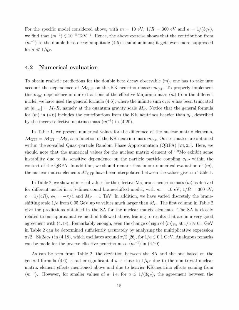
For the specific model considered above, with m = 10 eV, 1/R = 300 eV and a = 1/(3qF ),

we find that 〈m−1〉 <∼ 10−5 TeV−1. Hence, the above exercise shows that the contribution from

〈m−1〉 to the double beta decay amplitude (4.5) is subdominant; it gets even more suppressed

for a ≪ 1/qF .

4.2 Numerical evaluation

To obtain realistic predictions for the double beta decay observable 〈m〉, one has to take into

account the dependence of MGTF on the KK neutrino masses m(n). To properly implement

this m(n)-dependence in our extractions of the effective Majorana mass 〈m〉 from the different

nuclei, we have used the general formula (4.6), where the infinite sum over n has been truncated

at |nmax| = MFR, namely at the quantum gravity scale MF . Notice that the general formula

for 〈m〉 in (4.6) includes the contributions from the KK neutrinos heavier than qF , described

by the inverse effective neutrino mass 〈m−1〉 in (4.20).

In Table 1, we present numerical values for the difference of the nuclear matrix elements,

MGTF = MGT−MF, as a function of the KK neutrino mass m(n). Our estimates are obtained

within the so-called Quasi-particle Random Phase Approximation (QRPA) [24, 25]. Here, we

should note that the numerical values for the nuclear matrix element of 100Mo exhibit some

instability due to its sensitive dependence on the particle–particle coupling gPP within the

context of the QRPA. In addition, we should remark that in our numerical evaluation of 〈m〉,the nuclear matrix elements MGTF have been interpolated between the values given in Table 1.

In Table 2, we show numerical values for the effective Majorana-neutrino mass 〈m〉 as derivedfor different nuclei in a 5-dimensional brane-shifted model, with m = 10 eV, 1/R = 300 eV,

ε = 1/(4R), φh = −π/4 and MF = 1 TeV. In addition, we have varied discretely the brane-

shifting scale 1/a from 0.05 GeV up to values much larger than MF . The first column in Table 2

give the predictions obtained in the SA for the nuclear matrix elements. The SA is closely

related to our approximative method followed above, leading to results that are in a very good

agreement with (4.18). Remarkably enough, even the change of sign of 〈m〉SA at 1/a ≈ 0.1 GeV

in Table 2 can be determined sufficiently accurately by analyzing the multiplicative expression

π/2−Si(2aqF ) in (4.18), which oscillates around π/2 [26], for 1/a <∼ 0.1 GeV. Analogous remarks

can be made for the inverse effective neutrino mass 〈m−1〉 in (4.20).

As can be seen from Table 2, the deviation between the SA and the one based on the

general formula (4.6) is rather significant if a is close to 1/qF due to the non-trivial nuclear

matrix element effects mentioned above and due to heavier KK-neutrino effects coming from

〈m−1〉. However, for smaller values of a, i.e. for a <∼ 1/(3qF ), the agreement between the

18

m(n) [MeV] MGTF(m(n))

76Ge 82Se 100Mo 116Cd

≤ 1 4.33 4.03 4.86 3.29

10 4.34 4.04 4.81 3.29

102 3.08 2.82 3.31 2.18

103 1.40× 10−1 1.25× 10−1 1.60× 10−1 9.34× 10−2

104 1.39× 10−3 1.24× 10−3 1.60× 10−3 9.26× 10−4

105 1.39× 10−5 1.24× 10−5 1.60× 10−5 9.26× 10−6

106 1.39× 10−7 1.24× 10−7 1.60× 10−7 9.26× 10−8

107 1.39× 10−9 1.24× 10−9 1.60× 10−9 9.26× 10−10

m(n) [MeV] MGTF(m(n))

128Te 130Te 136Xe 150Nd

≤ 1 4.50 3.89 1.83 5.30

10 4.52 3.91 1.88 5.45

102 3.19 2.79 1.48 4.24

103 1.46× 10−1 1.29× 10−1 7.07× 10−2 2.02× 10−1

104 1.46× 10−3 1.28× 10−3 7.04× 10−4 2.02× 10−3

105 1.46× 10−5 1.28× 10−5 7.05× 10−6 2.02× 10−5

106 1.46× 10−7 1.28× 10−7 7.05× 10−8 2.02× 10−7

107 1.46× 10−9 1.28× 10−9 7.05× 10−10 2.02× 10−9

Table 1: QRPA estimates of the relevant combination of nuclear matrix elements, MGTF =

MGT −MF, as a function of the KK neutrino mass m(n).

effective neutrino mass computed in the SA and the general formula (4.6) is fairly good. In

this kinematic regime, the inverse effective neutrino mass 〈m−1〉 becomes rather suppressed

according to our discussion in (4.20). Our numerical estimates in the last column of Table 2

offer firm support of this last observation. Thus, the main contribution to 〈m〉 originates fromKK neutrinos much lighter than qF . Consequently, within the 5-dimensional brane-shifted

model, we have numerically established a sizeable value for 〈m〉 in the presently explorable

range 0.05–0.84 eV. Finally, for very small values of a, i.e. for a ≪ 1/MF , we recover the

undetectably small result (4.15) for the unshifted brane a = 0.

19

1/a 〈m〉 [eV] 〈m−1〉

[GeV] SA 76Ge 82Se 100Mo 116Cd 128Te 130Te 136Xe 150Nd [TeV−1]

0.05 –0.062 0.009 0.010 0.016 0.012 0.009 0.008 –0.004 –0.004 6.2×10−6

0.1 –0.012 0.052 0.054 0.061 0.062 0.052 0.050 0.025 0.026 –3.6×10−6

0.2 0.208 0.096 0.100 0.109 0.114 0.097 0.094 0.058 0.061 –1.3×10−5

0.3 0.307 0.123 0.128 0.136 0.143 0.124 0.121 0.082 0.086 –1.2×10−5

1 0.457 0.271 0.275 0.280 0.287 0.272 0.269 0.241 0.243 –5.7×10−6

10 0.516 0.493 0.493 0.494 0.495 0.493 0.493 0.489 0.489 –6.6×10−7

102 0.515 0.513 –6.7×10−8

103 0.535 –6.7×10−8

104 0.066 –6.9×10−10

1010 <∼ 10−6 0.

Table 2: Numerical estimates of 〈m〉 for different nuclei in a 5-dimensional brane-shifted model,

with m = 10 eV, 1/R = 300 eV, ε = 1/(4R), φh = −π/4 and MF = 1 TeV. The first column

exhibits the numerical values for 〈m〉 in the Step Approximation (SA) for the nuclear matrix

elements, while the last column shows the results for the inverse effective neutrino mass 〈m−1〉.

4.3 〈m〉 and the neutrino mass scale

Apart from explaining the recent excess in 0νββ decays, the 5-dimensional model with a

small but non-vanishing shifted brane exhibits another very important property. The effective

Majorana-neutrino mass 〈m〉 can be several orders of magnitude larger than the light neutrino

mass mν , for certain choices of the parameters ε and φh. To understand this phenomenon, let

us first consider the eigenvalue equation (2.27) for λ = mν , written in the form:

mν +∞∑

n=−∞

m(n)2

ε + nR

− mν

= 0 . (4.21)

Notice that (4.21) constitutes an excellent and very practical approximation of the neutrino-

mass–mixing sum rule, when the small mν-dependence in the infinite sum over the KK neutrino

states is neglected and the approximate formulae (4.4) and (4.16) for the KK masses m(n) and

mixing-matrix elements Be,n, along with Beν = 1, are substituted in (4.3). Then, the infinite

sum over KK neutrino states can be performed with the help of (2.28) for rational values of

a in πR units. Especially for a = πR/q with q being an integer much larger than 1, i.e. for

20

1/MF ≪ a <∼ 1/qF , the light neutrino mass mν is given by

mν ≈ − πm2R[

cos2 φh cot(πR ε) +1

2sin(2φh)

]

. (4.22)

It is now easy to see that the light neutrino mass mν can be very suppressed for specific values

of φh and ε. For instance, one obvious choice would be φh ≈ −π/4 and ε ≈ 1/(4R). On the

other hand, the effective neutrino mass 〈m〉SA is determined by the second sine-dependent term

in (4.22) (cf. (4.18)), which is induced by brane-shifting effects. Unlike the suppressed light

neutrino mass mν , the effective neutrino mass 〈m〉 can be sizeable in the observable range 0.05–

0.84 eV. This loss of correlation between the quantities 〈m〉 and mν is a rather unique feature of

our higher-dimensional brane-shifted scenario. As we will discuss in the next section, the above

de-correlation property plays a key role in our model-building of 5-dimensional brane-shifted

scenarios that could explain the neutrino oscillation data.

5 Atmospheric and solar neutrino data

Atmospheric and solar neutrino data [27,28,29], together with information from laboratory ex-

periments, such as the CHOOZ experiment [30], are very crucial for a given higher-dimensional

singlet-neutrino model to qualify as viable. In particular, the latest SNO results [28] appear

to disfavour large components of sterile neutrinos, indicating a preference among the different

solutions to the solar and atmospheric neutrino puzzles for those involving transitions between

almost active neutrinos.5 To account for this experimental indication, we assume that the

compactification scale 1/R and the lepton-number-violating bulk parameter ε are much larger

than the KK Dirac mass terms m(n) in (2.25).

In the following, we shall explicitly demonstrate that our 5-dimensional brane-shifted model

with only one bulk neutrino is able to fully explain the neutrino oscillation data. Specifically,

we will show that the preferred solar Large Mixing Angle (LMA) and atmospheric solutions,

which both require large νe-νµ and νµ-ντ mixings, can be realized within our 5-dimensional

model. These particular solutions are allowed, only if the differences of the squares of the light

neutrino masses lie in the ranges:

1.8×10−3 < ∆m2atm [eV2] < 4.0×10−3 , 2.0×10−5 < ∆m2

⊙ [eV2] < 2.0×10−4 , (5.1)

with ∆m2atm = m2

ν3− m2

ν2and ∆m2

⊙ = m2ν2

− m2ν1. According to the usual conventions, the

physical light neutrino masses mν1 , mν2 and mν3 are labelled in increasing hierarchical order,

i.e. mν1 ≤ mν2 ≤ mν3 .5A recent study [31] seems to suggest that the active neutrino component in the solar neutrinos has to be

larger than 86% at 1 σ CL. A loophole may exist for atmospheric neutrinos, see [32].

21

To start with, let us consider the weak basis in which the charged lepton mass matrix is

diagonal. Then, in the three-generation brane-shifted model, the KK-Dirac Yukawa terms are

given by the 3-vectors

m(n) =

me cos(naR

− φe)

mµ cos(naR

− φµ)

mτ cos(naR

− φτ )

, (5.2)

where

ml =v√2

√

(hl1)

2 + (hl2)

2 , φl = tan−1

(

hl2

hl1

)

+k0a

R, (5.3)

with l = e, µ, τ . Given our assumption that ε , 1/R ≫ ml, the KK neutrinos can now be

integrated out. Analogously with (2.27), the effective light neutrino mass matrix Mν can be

computed by

Mν = −+∞∑

n=−∞

m(n) m(n) T

nR

+ ε. (5.4)

Following the same line of steps as in Appendix A, one is able to analytically carry out the

infinite sum in (5.4) for the phenomenologically interesting case of a = πR/q, with q being an

integer much larger than 1. In this limit, we obtain the novel trigonometric mass texture:

Mνll′ = − πRmlml′

[

cosφl cosφl′ cot(πRε) +1

2sin(φl + φl′)

]

, (5.5)

with l, l′ = e, µ, τ . The effective neutrino mass matrix (5.5) consists of two terms: (i) the cosine-

dependent term that arises from the lepton-number-violating bulk mass M (or equivalently

ε) and (ii) the sine-dependent term which is due to lepton-number violation in the effective

Yukawa couplings and is caused by slightly shifting the brane from the orbifold fixed points.

The occurrence of the second brane-shifting mass term is always ensured as long as a ≫1/MF . Without the presence of this brane-shifting-induced term, the effective neutrino mass

matrix (5.5) is of rank 1, leading to two massless neutrinos. This last fact is very undesirable,

as it would be very difficult to explain both solar and atmospheric neutrino data with only

one non-trivial difference of neutrino masses in the frequently-discussed scenario without brane

shifting.

As has been discussed in Section 4, however, even a small amount of brane shifting may in-

duce sizeable lepton-number-violating Yukawa interactions. The latter generate brane-shifting

mass terms that break the rank-1 structure of the effective neutrino mass matrix Mν . The

resulting Mν in (5.5) exhibits a novel trigonometric structure that can predict hierarchical

neutrinos with large νµ–ντ and νµ–νe mixings to explain the atmospheric and solar neutrino

anomalies, along with a small νe–ντ mixing as required by the CHOOZ experiment [30]. At this

point, it is important to stress that the effective neutrino mass 〈m〉 entering the 0νββ-decay

22

amplitude gets fully decoupled from the neutrino-mass matrix element Mνee. According to our

discussions in Section 4 (cf. (4.18)), the effective neutrino mass for the three-generation case is

given by

〈m〉 ≈ −1

2sin(2φe) π(m

e)2R 6= Mνee . (5.6)

It is important to recall again that unlike Mνee, KK neutrinos heavier than the Fermi nuclear

momentum qF do not contribute significantly to 〈m〉, leading to the loss of correlation between

〈m〉 and Mνee. The latter is a distinctive feature of the KK-neutrino dynamics. This de-

corellation between 〈m〉 and Mνee permit us to consider the interesting case |〈m〉| ≫ |Mν

ll′|,for all l, l′ = e, µ, τ . Such a realization enables us to accommodate a sizeable positive signal of

0νββ decays together with the present neutrino oscillation data.

To realize the aforementioned hierarchy |〈m〉| ≫ |Mνll′|, we assume that all phases φl are

close to −π/4. For concreteness, we adopt the following scheme of phases:

φl = − π

4+ δl , πRε =

π

4− δε . (5.7)

where δl, δε ≪ 1. Our choice of phases has been motivated by the fact that the above-described

de-correlation between 〈m〉 and Mνee becomes fully operative in this case. To implement the

CHOOZ constraint in our model-building, we require thatMνeτ = Mν

τe = 0. This last constraint

implies that

2δε = −δe − δτ . (5.8)

Moreover, without loss of generality within our phase scheme, we may take δµ = 0. Under these

assumptions, the light neutrino-mass matrix takes on the simple form

Mν =πR

2

me 2 (δτ − δe) memµ δτ 0

mµme δτ mµ 2 (δe + δτ ) mµmτ δe

0 mτmµ δe mτ 2 (δe − δτ )

. (5.9)

Let us now consider the following numerical example:

δτ = δ , δe = 2δ ,mµ

me≈ 1.468 ,

mτ

me≈ 2.542 . (5.10)

This leads to the neutrino mass matrix:

Mν = δπme 2R

2

−1 1.47 0

1.47 6.46 7.46

0 7.46 6.46

. (5.11)

Notice that all elements of the neutrino-mass matrixMν in (5.11) can be suppressed by choosing

a small value for the factorizable parameter δ. In our numerical example, the neutrino mass

23

matrix (5.11) can be diagonalized through νµ-ντ and νe-νµ mixing angles close to π/4, whereas

the νe-ντ mixing angle is small, below 0.1. In addition, its mass-eigenvalues are approximately

given by

(Mν)diag ≈ δ πme 2R(

0 , 1 , 7)

. (5.12)

Assuming thatme = 10 eV and 1/R = 300 eV for a successful interpretation of the recent excess

in 0νββ decays, then it should be δ = (6–9) × 10−3 to accommodate the neutrino oscillation

data through the LMA solution. In particular, we obtain the neutrino-mass differences:

∆m2atm ≈ (2− 4)× 10−3 eV2 , ∆m2

⊙ ≈ (4− 8)× 10−5 eV2 (5.13)

These results are fully compatible with the currently preferred atmospheric and solar LMA

solutions to the neutrino anomalies.

In our demonstrative analysis carried out in this section, we have not attempted to fit

the results of the Liquid Scintillator Neutrino Detector (LSND) as well [33]. In principle, our

brane-shifted 5-dimensional models are capable of accommodating the LSND results through

active-sterile neutrino transitions. In this case, however, the lowest-lying KK singlet neutrinos

should be relatively light. As a result, they cannot be integrated out from the light neutrino

spectrum, thereby leading to a much more involved effective neutrino-mass matrix. A complete

study of this issue, including possible constraints from the cooling of supernova SN1987A [8,34],

is beyond the scope of the present paper and may be given elsewhere.

6 Conclusions

We have studied the model-building constraints derived from the requirement that KK singlet

neutrinos in theories with large extra dimensions can give rise to a sizeable 0νββ-decay signal

to the level of 0.4 eV reported recently. Our analysis has been focused on 5-dimensional

S1/Z2 orbifold models with one sterile (singlet) neutrino in the bulk, while the SM fields are

considered to be localized on a 3-brane. In our model-building, we have also allowed the 3-

brane to be displaced from the S1/Z2 orbifold fixed points. Within this minimal 5-dimensional

brane-shifted framework, lepton-number violation can be introduced through Majorana-like

bilinears, which may or may not arise from the Scherk–Schwarz mechanism, and through lepton-

number-violating Yukawa couplings. However, lepton-number-violating Yukawa couplings can

be admitted in the theory, only if the 3-brane is shifted from the S1/Z2 orbifold fixed points.

Apart from a possible stringy origin [20], brane-shifting might also be regarded as an effective

result owing to a non-trivial 5-dimensional profile of the Higgs particle [35] and/or other SM

24

fields [36, 37] that live in different locations of a 3-brane with non-zero thickness which is

centered at one of the S1/Z2 orbifold fixed points.

One major difficulty of the higher-dimensional theories is their generic prediction of a KK

neutrino spectrum of approximately degenerate states with opposite CP parities that lead to

exceedingly suppressed values for the effective Majorana-neutrino mass 〈m〉. Nevertheless,

we have shown that within the 5-dimensional brane-shifted framework, the KK neutrinos can

couple to the W± bosons with unequal strength, thus avoiding the disastrous CP-parity can-

cellations in the 0νββ-decay amplitude. In particular, the brane-shifting parameter a can be

determined from the requirement that the effective Majorana mass 〈m〉 is in the observable

range [13]: 0.05–0.84 eV. In this way, we have found that 1/a has to be larger than the typical

Fermi nuclear momentum qF = 100 MeV and much smaller than the quantum gravity scale

MF , or equivalently 1/MF ≪ a <∼ 1/qF .

An important prediction of our 5-dimensional brane-shifted model is that the effective

Majorana-neutrino mass 〈m〉 and the scale of light neutrino masses can be completely de-

correlated for certain natural choices of the Majorana-like bilinear term ε and the original

5-dimensional Yukawa couplings hl1 and hl

2 in (2.4). For example, if ε ≈ 1/(4R) and hl1 ≈ −hl

2,

we obtain light-neutrino masses that can be several orders of magnitude smaller than 〈m〉.Nevertheless, it is worth mentioning that if future data did not substantiate the presently re-

ported 0νββ excess, the above model-building conditions would then need be modified. Such

a possible modification would not jeopardize though the viability of our brane-shifted scenario.

Indeed, if the upper limit on the effective neutrino mass became even lower and lower, this

would imply that the above decorrelation property is less and less necessary.

Another important prediction of the 5-dimensional brane-shifted model with only one bulk

sterile neutrino is that the emerging effective light-neutrino mass matrix does no longer possess

the rank-1 form, as opposed to the brane-unshifted a = 0 case. As we have shown in Section 5,

the above properties of the brane-shifted models are sufficient to explain, even with only one

neutrino in the bulk, the present solar and atmospheric neutrino data by means of oscillations

of hierarchical neutrinos with large νe-νµ and maximal νµ-ντ mixings. In particular, neutrino-

mass textures can be constructed that utilize the currently preferred LMA solution, where the

νe-ντ mixing is small in agreement with the CHOOZ experiment.

Although a sizeable 0νββ-decay signal can be predicted within our brane-shifted 5-

dimensional models, the above-described de-correlation property between 〈m〉 and the actual

light neutrino masses suggests, however, that it is rather unlikely that such a signal be accompa-

nied by a corresponding signal in Tritium beta-decay experiments. For example, the KATRIN

project [38] has a sensitivity to active neutrino masses larger than 0.35 eV at 95% CL, and so

25

it can only probe the existence of light neutrinos much heavier than those considered in our

5-dimensional models. Finally, the brane-shifted models under study also have the potential to

accommodate the LSND results by virtue of active-sterile neutrino oscillations. In this case,

the lowest-lying KK-neutrino states will contribute to the effective light neutrino-mass matrix,

giving rise to more involved mass textures. In this context, it would be very interesting to

investigate the question whether a simple higher-dimensional model accounting for all the ob-

served neutrino anomalies can be established. We plan to address this interesting question in

the near future.

Acknowledgements

We thank Martin Hirsch for discussions on QRPA computations and Antonio Delgado for

comments on the geometric breaking of lepton number violation in higher-dimensional theories.

26

A Eigenvalue equation

Starting from (2.27), we will derive here the transcendental eigenvalue equation (2.28), for the

simplest class of brane-shiftings with a = πR/q, where r = 1 and q is an integer larger than 1,

i.e. q ≥ 2. Then, the eigenvalue equation (2.27) can be equivalently written as

λ =q−1∑

l=0

∞∑

k=−∞

m(qk+l) 2

λ− ε− qk+lR

=q−1∑

l=0

m(l) 2∞∑

k=−∞

1

λ− ε− qk+lR

, (A.1)

where we have used the periodicity property (m(l))2 = (m(qk+l))2 in the second step of (A.1).

In fact, it is this last periodicity property of the KK-Yukawa terms that we wish to exploit

here to carry out analytically the infinite sums in (A.1), which has forced us to introduce the

technical constraint (2.23), namely that a/(πR) is a rational number. Now, the individual l-

dependent infinite sums over k in (A.1) can be performed independently, using complex contour

integration techniques. In this way, we obtain

λ =1

qπm2R

q−1∑

l=0

cos2(

φh − lπ

q

)

cot[

1

qπR (λ− ε) − lπ

q

]

. (A.2)

Our next task is to carry out the summation over l in (A.2). For this purpose, we express

the RHS of (A.2) entirely in terms of sine and cosine functions by factoring out the common

divisor, i.e.

λ =πm2R

qq−1∏

l=0sin

(

θq− lπ

q

)

q−1∑

l=0

cos2(

φh − lπ

q

)

cos(

θ

q− lπ

q

) q−1∏

m=0(m6=l)

sin(

θ

q− mπ

q

)

, (A.3)

with θ = πR (λ−ε). To further evaluate (A.3), we exploit the following trigonometric identities:6

q−1∏

l=0

sin(

θ

q− lπ

q

)

=(−1)q−1

2q−1sin θ , (A.4)

q−1∑

l=0

cos(

θ

q− lπ

q

) q−1∏

m=0(m6=l)

sin(

θ

q− mπ

q

)

=(−1)q−1

2q−1q cos θ , (A.5)

q−1∑

l=0

cos(

2φh − 2lπ

q

)

cos(

θ

q− lπ

q

) q−1∏

m=0(m6=l)

sin(

θ

q− mπ

q

)

=

(−1)q−1

2q−1q cos

(

2φh +q − 2

qθ)

. (A.6)

6The proof of these identities is rather lengthy and relies on the particular properties of the q-roots of the

unity, i.e. the roots of the equation zq = 1. Specifically, we used the basic property of the unit roots that their

sum and the sum of their products are zero, while their total product is (−1)q−1.

27

With the help of (A.4)–(A.5), we arrive at the transcendental eigenvalue equation

λ =πm2R

2

{

cot[

πR (λ− ε)]

+cos

[

2φh + q−2q

πR (λ− ε)]

sin[

πR (λ− ε)]

}

. (A.7)

If we replace q with πR/a in (A.7), we arrive after simple trigonometric algebra at the tran-

scendental eigenvalue equation (2.28). Although we focused our attention on the simplest class

with a = πR/q, we should remark that our methodology described above can apply equally

well to the most general case where the brane-shifting a is any rational number r/q in πR units.

B Sum rules

In this appendix, we will show that the KK-neutrino masses determined by the roots of (2.21)

and the mixing-matrix elements given in (4.11) satisfy the sum rules (4.2) and (4.3). For

simplicity, we consider the case a = 0. However, our considerations carry over very analogously

to the case a = πR/q 6= 0, where q is an integer larger than 1.

Let us first consider (4.2) for l = l′ = e. We will then prove that

|Beν |2 + limN→∞

N∑

n=−N

|Be,n|2 = 1 . (B.1)

Our proof will rely on Cauchy’s integral theorem. Thus, the LHS of (B.1) can be expressed in

terms of a complex integral as follows:

|Beν |2 + limN→∞

N∑

n=−N

|Be,n|2 =1

2πilim

N→∞

∮

CN

dz(

1

z −mν

+N∑

n=−N

1

z −m(n)

)

× 1

1 + π2m2R2/ sin2[πR(z − ε)]

=1

2πilim

N→∞

∮

CN

dz1

z − πm2R cot[πR(z − ε)]. (B.2)

In deriving the second equality in (B.2), we have noticed that for z in the vicinity of the pole,

e.g. for z ≈ m(n), it is

z − πm2R cot[πR(z − ε)] ≈ (z −m(n)){

1 +π2m2R2

sin2[πR(z − ε)]

}

. (B.3)

Such a substitution is only valid under complex integration, provided there are no singularities

of the complex function cot[πR(z − ε)] on the contour CN . For this purpose, we choose our

28

contours to be circles represented in the complex plane as

zN =(N + 1

2) eiθ

R+ ε . (B.4)

Then, it can be shown that on the complex contours z = zN , | cotπR(zN − ε)| is bounded

from above by a constant independent of N . Thus, on CN the last integral in (B.2) may be

successively computed as

1

2πilim

N→∞

∮

CN

dz1

z − πm2R cot[πR(z − ε)]

=1

2πilim

N→∞

∫ 2π

0dθ

i(zN − ε)

zN − πm2R cot[π(N + 12) eiθ]

= 1 +1

2πlim

N→∞

∫ 2π

0dθ

πm2R cot[π(N + 12) eiθ] − ε

zN − πm2R cot[π(N + 12) eiθ]

. (B.5)

The second term in the last equality of (B.5) vanishes in the limit N → ∞ or equivalently when

zN is taken to infinity in a discrete manner as prescribed by (B.4). Thus, the complex integral

in the last equality of (B.2) is exactly 1, which proves the unitarity sum rule (B.1).

In the remainder of the appendix, we will prove the neutrino-mass-mixing sum rule:

B2eν mν + lim

N→∞

N∑

n=−N

B2e,n m(n) = 0 . (B.6)

In our proof, we will follow a path very analogous to the one outlined above for showing (B.1).

Thus, the LHS of (B.6) may be expressed in terms of a complex integral as follows:

B2eν mν + lim

N→∞

N∑

n=−N

B2e,nm(n) =

1

2πilim

N→∞

∮

CN

dzz

z − πm2R cot[πR(z − ε)]. (B.7)

Evaluating the complex integral on the contours CN defined by (B.4) yields

1

2πilim

N→∞

∮

CN

dzz

z − πm2R cot[πR(z − ε)]

=1

2πilim

N→∞

∫ 2π

0dθ

i(zN − ε) πm2R cot[π(N + 12) eiθ]

zN − πm2R cot[π(N + 12) eiθ]

=1

2m2R lim

N→∞

{∫ 2π

0dθ cot[π(N + 1

2) eiθ] + O(1/zN)

}

. (B.8)

Similar to the second term in the last equality of (B.8), which goes to zero for N → ∞, the

first term vanishes as well after integration over θ. This can be readily seen by exploiting

29

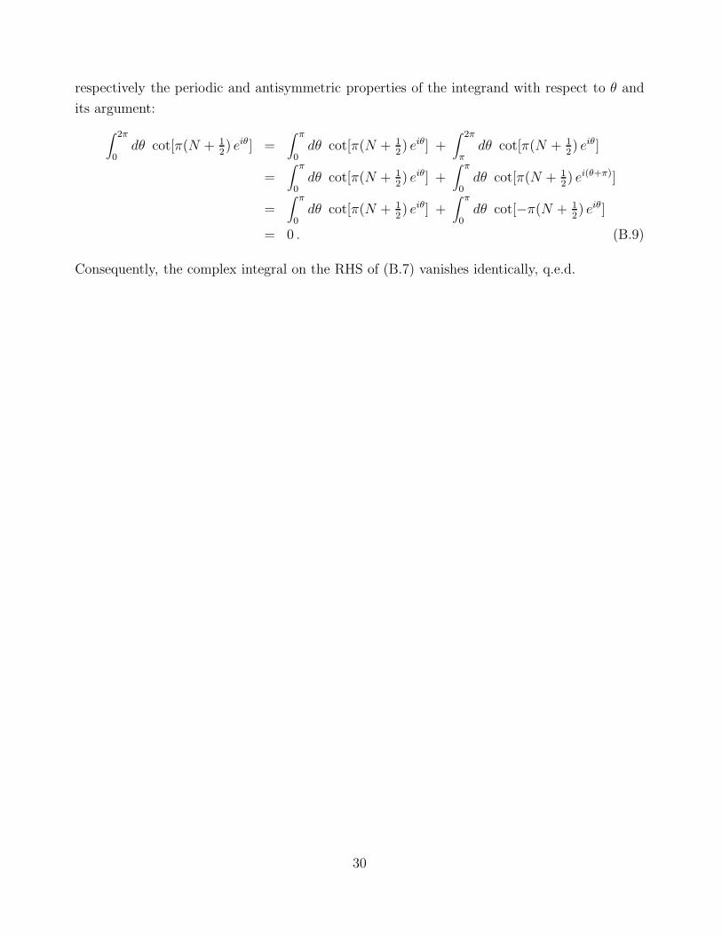
respectively the periodic and antisymmetric properties of the integrand with respect to θ and

its argument:

∫ 2π

0dθ cot[π(N + 1

2) eiθ] =

∫ π

0dθ cot[π(N + 1

2) eiθ] +

∫ 2π

πdθ cot[π(N + 1

2) eiθ]

=∫ π

0dθ cot[π(N + 1

2) eiθ] +

∫ π

0dθ cot[π(N + 1

2) ei(θ+π)]

=∫ π

0dθ cot[π(N + 1

2) eiθ] +

∫ π

0dθ cot[−π(N + 1

2) eiθ]

= 0 . (B.9)

Consequently, the complex integral on the RHS of (B.7) vanishes identically, q.e.d.

30

References

[1] N. Arkani-Hamed, S. Dimopoulos and G. Dvali, Phys. Lett. B429 (1998) 263; I. Anto-

niadis, N. Arkani-Hamed, S. Dimopoulos and G. Dvali, Phys. Lett. B436 (1998) 257;

K.R. Dienes, E. Dudas and T. Gherghetta, Phys. Lett. B436 (1998) 55; Nucl. Phys. B537

(1999) 47; L. Randall and R. Sundrum, Phys. Rev. Lett. 83 (1999) 3370. For earlier stud-

ies, see I. Antoniadis, Phys. Lett. B246 (1990) 377; J.D. Lykken, Phys. Rev. D54 (1996)

3693; P. Horava and E. Witten, Nucl. Phys. B460 (1996) 506; Nucl. Phys. B475 (1996) 94.

[2] K.R. Dienes, E. Dudas and T. Gherghetta, Nucl. Phys. B557 (1999) 25.

[3] N. Arkani-Hamed, S. Dimopoulos, G. Dvali and J. March-Russell, hep-ph/9811448.

[4] G. Dvali and A. Yu. Smirnov, Nucl. Phys. B563 (1999) 63.

[5] A. Pilaftsis, Phys. Rev. D60 (1999) 105023.

[6] A. Ioannisian and A. Pilaftsis, Phys. Rev. D62 (2000) 066001; A.E. Faraggi and

M. Pospelov, Phys. Lett. B458 (1999) 237; G.C. McLaughlin and J.N. Ng, Phys. Rev.

D63 (2001) 053002; K. Agashe and G. H. Wu, Phys. Lett. B498 (2001) 230; B. He,

T.P. Cheng and L.F. Li, hep-ph/0209175.

[7] R.N. Mohapatra, S. Nandi and A. Perez-Lorenzana, Phys. Lett. B466 (1999) 115;

R.N. Mohapatra and A. Perez-Lorenzana, Nucl. Phys. B576 (2000) 466; R. Barbieri,

P. Creminelli and A. Strumia, Nucl. Phys. B585 (2000) 28; Y. Grossman and M. Neubert,

Phys. Lett. B474 (2000) 361; A. Ioannisian and J.W.F. Valle, Phys. Rev. D63 (2001)

073002; D.O. Caldwell, R.N. Mohapatra and S.J. Yellin, Phys. Rev. D64 (2001) 073001;

K.R. Dienes and I. Sarcevic, Phys. Lett. B500 (2001) 133; A. de Gouvea, G.F. Giudice,

A. Strumia and K. Tobe, Nucl. Phys. B623 (2002) 395.

[8] A. Lukas, P. Ramond, A. Romanino and G.G. Ross, JHEP 0104 (2001) 010.

[9] H. Davoudiasl, P. Langacker and M. Perelstein, Phys. Rev. D65 (2002) 105015.

[10] M. Doi, T. Kotani and E. Takasugi, Prog. Theor. Phys. Suppl. 83 (1985) 1.

[11] For example, see the textbook by K. Grotz and H.V. Klapdor, “The Weak Interaction in

Nuclear, Particle und Astrophysics,” (Adam Hilger, Bristol, 1989).

[12] H.V. Klapdor-Kleingrothaus, “Sixty Years of Double Beta Decay,” (World Scientific, Sin-

gapore, 2001).

31

[13] H.V. Klapdor-Kleingrothaus, A. Dietz, H.L. Harney, I.V. Krivosheina, Mod. Phys. Lett.

A16 (2001) 2409; H.V. Klapdor-Kleingrothaus, A. Dietz and I. Krivosheina, Particles and

Nuclei 110 (2002) 57; Foundations of Physics 32 (2002) 1181.

[14] H.V. Klapdor-Kleingrothaus and U. Sarkar, Mod. Phys. Lett. A16 (2001) 2469;

H.V. Klapdor-Kleingrothaus, H. Pas and A. Yu. Smirnov, Phys. Rev. D63 (2001) 073005;

hep-ph/0103076; W. Rodejohann, Nucl. Phys. B597 (2001) 110; J. Phys. G28 (2002) 1477;

H. Minakata and H. Sugiyama, Phys. Lett. B532 (2002) 275; S. Pascoli and S.T. Petcov,

Phys. Lett. B544 (2002) 239; H. Nunokawa, W.-J. Teves and R. Zukanovich Funchal,

hep-ph/0206137.

[15] R.N. Mohapatra, A. Perez-Lorenzana and C.A. de S. Pires, Phys. Lett. B491 (2000) 143.

[16] S.J. Huber and Q. Shafi, Phys. Lett. B544 (2002) 295.

[17] J. Scherk and J.H. Schwarz, Phys. Lett. B82 (1979) 60; Nucl. Phys. B153 (1979) 61;

P. Fayet, Phys. Lett. B159 (1985) 121; Nucl. Phys. B263 (1986) 649.

[18] L. Wolfenstein, Phys. Rev. D17 (1978) 2369; S.P. Mikheev and A.Y. Smirnov, Sov. J.

Nucl. Phys. 42 (1985) 913 [Yad. Fiz. 42 (1985) 1441].

[19] A. Delgado, G. v. Gersdorff and M. Quiros, hep-th/0210181; see, also, J.A. Bagger,

F. Feruglio and F. Zwirner, Phys. Rev. Lett. 88 (2002) 101601.

[20] For example, see, E.G. Gimon and J. Polchinski, Phys. Rev. D54 (1996) 1667.

[21] P.H. Chankowski and S. Pokorski, Int. J. Mod. Phys. A17 (2002) 575.

[22] See A. Ioannisian and A. Pilaftsis in [6].

[23] M. Hirsch and H.V. Klapdor-Kleingrothaus, in Proc. “Double Beta Decay and Related

Topics,” Trento 1995, World Scientific, p. 175.

[24] K. Muto, E. Bender and H.V. Klapdor, Z. Phys. A334 (1989) 187.

[25] A. Staudt, K. Muto and H.V. Klapdor-Kleingrothaus, Europhys. Lett. 13 (1990) 31;

M. Hirsch, K. Muto, T. Oda and H.V. Klapdor-Kleingrothaus, Z. Phys. A347 (1994)

151.

[26] See, e.g., M. Abramowitz and I.A. Stegun, “Handbook of Mathematical Functions,” (Ver-

lag Harri Deutsch, Frankfurt, 1984), p. 60.

32

[27] Super-Kamiokande Collaboration (Y. Fukuda et. al.), Phys. Rev. Lett. 81 (1998) 1562;

Phys. Lett. B433 (1998) 9; Phys. Rev. Lett. 85 (2000) 3999.

[28] SNO Collaboration (Q.R. Ahmad et. al.), Phys. Rev. Lett. 87 (2001) 071301; Phys. Rev.

Lett. 89 (2002) 011301.

[29] G. Altarelli and F. Feruglio, Phys. Rept. 320 (1999) 295; hep-ph/0206077; J.N. Bahcall,

P.I. Krastev and A. Yu. Smirnov, JHEP 05 (2001) 015; G.L. Fogli, E. Lisi, A. Mar-

rone and A. Palazzo, Phys. Rev. D64 (2001) 093007; A. Bandyopadhyay, S. Choubey

S. Goswami and K. Kar, Phys. Lett. B519 (2001) 83; J.N. Bahcall, M.C. Gonzalez-

Garcia and C. Pena-Garay, JHEP 0207 (2002) 054; P.C. de Holanda and A. Yu. Smirnov,

hep-ph/0205241; M. Maltoni, T. Schwetz, M. A. Tortola and J. W. Valle, Nucl. Phys. Proc.

Suppl. 114 (2003) 203 [arXiv:hep-ph/0209368]; M. Maltoni, T. Schwetz and J. W. Valle,

arXiv:hep-ph/0212129.

[30] CHOOZ Collaboration (M. Apollonio et. al.), Phys. Lett. B466 (1999) 415.

[31] P.C. de Holanda and A.Yu. Smirnov, hep-ph/0211264.

[32] H. Pas, L. Song, T.J. Weiler, hep-ph/0209373.

[33] LSND Collaboration (C. Athanasopoulos et. al.), Phys. Rev. Lett. 77 (1996) 3082; Phys.

Rev. Lett. 81 (1998) 1774.

[34] S. Hannestad, P. Keranen and F. Sannino, Phys. Rev.D66 (2002) 045002; G. Cacciapaglia,

M. Cirelli, Y. Lin and A. Romanino, hep-ph/0209063.

[35] V.A. Rubakov and M.E. Shaposhnikov, Phys. Lett. B125 (1983) 136.

[36] N. Arkani-Hamed and M. Schmaltz, Phys. Rev. D61 (2000) 033005; E.A. Mirabelli and

M. Schmaltz, Phys. Rev. D61 (2000) 113011; G. Dvali and M. Shifman, Phys. Lett. B475

(2000) 295; G.C. Branco, A. de Gouvea and M.N. Rebelo, Phys. Lett. B506 (2001) 115;

M. Raidal and A. Strumia, hep-ph/0210021.

[37] H.V. Klapdor–Kleingrothaus and U. Sarkar, Phys. Lett. B541 (2002) 332.

[38] KATRIN Collaboration (C. Weinheimer et al.), Prog. Part. Nucl. Phys. 48 (2002) 141.

33